A Hybrid Scheme for Encoding Audio Signal using Hidden Markov Models of Waveforms

Abstract.

This paper reports on recent results related to audiophonic signals encoding using time-scale and time-frequency transform. More precisely, non-linear, structured approximations for tonal and transient components using local cosine and wavelet bases will be described, yielding expansions of audio signals in the form tonal + transient + residual. We describe a general formulation involving hidden Markov models, together with corresponding rate estimates. Estimators for the balance transient/tonal are also discussed.

1. Introduction: structured hybrid models

Recent signal processing studies have shown the importance of sparse representations for various tasks, including signal and image compression (obviously), de-noising, signal identification/detection,… Such sparse representations are generally achieved using suitable orthonormal bases of the considered signal space. However, recent developments also indicate that redundant systems, such as frames, or more general “waveform dictionaries” may yield substantial gains in this context, provided that they are sufficiently adapted to the signal/image to be described.

From a different point of view, it has also been shown by several authors that in a signal or image compression context, significant improvements may be achieved by introducing structured approximation schemes, namely schemes in which structured sets of coefficients are considered rather than isolated ones.

The goal of this paper is to describe a new approach that implements both ideas, via a hybrid model involving sparse, structured, random wavelet/MDCT expansions, where the sets of considered coefficients (the significance maps) are described via suitable (hidden) Markov models.

This work is mainly motivated by audio coding applications, to which we come back after describing the models and corresponding estimation algorithms. However, similar ideas may clearly be developed in different contexts, including image [20] and image sequence coding, where both ingredients (hybrid and structured models) have already been exploited.

1.1. Generalities, sparse expansions in redundant systems

Very often, signals turn out to be made of several components, of significantly different nature. This is the case for “natural images”, which may contain edge information, regular textures, and “non-stationary” textures (which carry 3D information.) This is also the case for audio signals, which among other features, contain transient and tonal components [7], on which we shall focus more deeply. It is known that such different features may be represented efficiently in specific orthonormal bases. Following the philosophy of transform coding, this suggests to consider redundant systems made out by concatenation of several families of bases. Such systems have been considered for example in [9, 12, 14], where the problem of selecting the “sparsest” expansion through linear programing has been considered.

Focusing on the particular application to audio signals, and limiting ourselves to transient and tonal features, we are naturally led to consider a generic redundant dictionary made out of two orthonormal bases, denoted by $\psi_{\lambda}$ and $w_{\delta}$ respectively (typically a wavelet and an MDCT basis), and signal expansions of the form

(1) $$x=\sum_{\lambda\in\Lambda}\alpha_{\lambda}\psi_{\lambda}+\sum_{\delta\in\Delta}\beta_{\delta}w_{\delta}+r\ ,$$

where $\Lambda$ and $\Delta$ are (small, and this will be the main sparsity assumption) subsets of the index sets, hereafter termed significance maps. The nonzero coefficients $\alpha_{\lambda}$ are independent ${\mathcal{N}}(0,\sigma_{\lambda}^{2})$ random variables, and the nonzero coefficients $\beta_{\delta}$ are independent ${\mathcal{N}}(0,{\tilde{\sigma}}_{\delta}^{2})$ random variables: $r$ is a residual signal, which is not sparse with respect to the two considered bases (we shall talk of spread residual), and is to be neglected or described differently.

The approach developed in [9, 12, 14] may be criticized in several respects when it comes to practical implementation in a coding perspective. On one hand, it is not clear that the corresponding linear programing algorithms are compatible with practical constraints, in terms of CPU and memory requirements. Also, models exploiting solely sparsity arguments cannot capture one of the main features of some signal classes, namely the persistence property: significant coefficients have a tendency to form “clusters”, or “structured sets”. For example, in an audio coding context, the significance maps take the form of ridges (i.e. “time-persistent” sets, see e.g. [2, 8] in a different context) for the MDCT map $\Delta$, and binary trees for the wavelet map $\Lambda$. This remark has been exploited in various instances, for example in the context of the sinusoidal models for speech [19], of for image coding [4, 5, 25, 26]

Several models may be considered for the $\Lambda$ and $\Delta$ sets (termed significance maps), with variable levels of complexity. If only sparsity is used, they may be chosen uniformly distributed (in a finite dimensional context.) We shall rather work in a more complex context, and use (hidden) Markov chains to describe the MDCT ridges in $\Delta$ (in the spirit of the sinusoidal models of speech), and (hidden) binary Markov trees for the wavelet map $\Lambda$, following [5]. This not only yields a better modeling of the features of the signal, but also provides corresponding estimation algorithms.

To be more specific, a tonal signal is modeled as

$$x_{ton}=\sum_{\delta\in\Delta}\beta_{\delta}w_{\delta}\ ,$$

the functions $w_{\delta}$ being local cosine functions. The (significant) coefficients $\beta_{\delta}$, $\delta\in\Delta$ are ${\mathcal{N}}(0,{\tilde{\sigma}}_{\delta}^{2})$ independent random variables. The index $\delta$ is in fact a pair of time-frequency indices $\delta=(k,\nu)$, and the significance map $\Delta$ is characterized by a “fixed frequency” Markov chain (see e.g. [16] for a simple account), hence by a set of initial frequencies $\nu_{1},\dots\nu_{N}$ and transitions matrices ${\tilde{P}}_{1},\dots\tilde{P}_{N}$ (one for each frequency bin).

Globally, the tonal model is characterized by the set of matrices ${\tilde{P}}_{n}$, and the variances ${\tilde{\sigma}}_{\delta}^{2}$ of the two states, which are assumed to be time invariant, and on which additional constraints may be imposed. The tonal model is described in some details in section 2.

A similar model, using Hidden Markov trees of wavelet coefficients [5] may be develop to describe the transient layer in the signal:

$$x_{tr}=\sum_{\lambda\in\Lambda}\alpha_{\lambda}\psi_{\lambda}\ ,$$

$\psi$ being a wavelet with good time localization. The rationale is now to model the scale persistence of large wavelet coefficients of the transients, exploiting the intrinsic dyadic tree structure of wavelet coefficients (see Figure 5 below.) Again, the significant wavelet coefficients $\{\alpha_{\lambda},\lambda\in\Lambda\}$ of the signal are modeled as independent ${\mathcal{N}}(0,\sigma_{\lambda}^{2})$ random variables. The index $\lambda$ is in fact a pair of scale-time indices $\delta=(j,k)$, and the significance map $\Lambda$ is characterized by a “fixed time” Markov chain, hence by corresponding “scale to scale” transition matrices $P_{j}$ (with additional constraints which ensure that significant coefficients inherit a natural tree structure, see below.)

The transient model is therefore characterized by the variances of wavelet coefficients in $\Lambda$ and $\Lambda^{c}$, and the persistence probabilities, for which estimators may be constructed. The transient states estimation itself is also performed via classical methods. These aspects are described in section 3.

1.2. Recursive estimation

Several approaches are possible to estimate the significance maps and corresponding coefficients in models such as (1), ranging from the above mentioned linear programing schemes (see for example [3]) to greedy algorithms, including for instance Matching pursuit [13, 18]. The procedure we use is in some sense intermediate between these two extremes, in the spirit of the techniques used in [1]. We consider a dictionary made of two (orthonormal) bases; a first layer is estimated, using the first basis, and a second layer is estimated from the residual, using the second basis. The main difficulty of such an approach lies on the fact that the number of significant elements from the first basis has to be known in advance (or at least estimated.) In other terms, the cardinalities $|\Lambda|$ and $|\Delta|$ of the significance maps have to be known. This is important, since an underestimation or overestimation of $|\Delta|$ (assuming that the $\Delta$-layer is estimated first) will “propagate” to the estimation of the second layer (the $\Lambda$-layer.)

In the framework of the the Gaussian random sparse models studied below, it is possible to derive a priori estimates for the cardinalities $|\Lambda|$ and $|\Delta|$, using information measures in the spirit of those proposed in [30] and studied in [27]. Consider the geometric means of estimated $\psi_{\lambda}$ and $w_{\delta}$ coefficients

(2) $$\hat{N}_{\psi}=\left(\prod_{n=1}^{N}|\langle x,\psi_{n}\rangle|^{2}\right)^{1/N}\ \hbox{and }\qquad\hat{N}_{w}=\left(\prod_{n=1}^{N}|\langle x,w_{n}\rangle|^{2}\right)^{1/N}\ .$$

Then, assuming spartity, the indices

(3) $$I_{w}=\frac{\hat{N}_{\psi}}{\hat{N}_{\psi}+\hat{N}_{w}}\ ;\qquad I_{\psi}=\frac{\hat{N}_{w}}{\hat{N}_{\psi}+\hat{N}_{w}}\ ,$$

turn out to provide estimates for the proportion of significant $w$ and $\psi$ coefficients. The rationale is the fact that under sparsity assumptions (i.e. if $\Delta$ and $\Lambda$ are small enough), most coefficients $\langle x,\psi_{n}\rangle$ (resp. $\langle x,w_{n}\rangle$) will come from the tonal (resp. transient) layer of the signal, and therefore give information about it. This aspect is discussed in more details in section 4.

1.3. Audio coding applications

As mentioned earlier, the primary motivation for this work was audio coding. We briefly sketch here the assets of the model we are developing in such a context.

Coding involve (lossy) quantization of the selected coefficients $\{\langle x,w_{\delta}\rangle,\delta\in\Delta\}$ and $\{\langle x,\psi_{\lambda}\rangle,\lambda\in\Lambda\}$. These are Gaussian random variables, which means that corresponding rate and distortion estimates may be obtained. We notice that the introduction of structured significance maps does not improve the quality of the approximation (as measured by $L^{2}$ distortion); however it improves the efficiency of significance map encoding (see below); in addition, for audio applications, since structured significance maps seem to be relevant in the sense that they describe more accurately elementary “sound objects”, they often yield better approximations of audio signals, from perceptual points of view.

Besides coefficients, significance maps have to be encoded as well. However, the Markov models make it possible to compute explicitly the probabilities of ridges lengths (for $\Delta$) and trees sizes, which allows one to obtain directly the corresponding optimal lossless code. Again, rate estimates may be derived explicitly.

It is also worth pointing out some important issues (in a coding perspective), which we shall not address here. The first one is the encoding of the residual signal

$$x_{res}=x-x_{ton}-x_{tr}\ .$$

It was suggested in [7] that the residual may be encoded using standard LPC techniques. However, it appears that in most situations (at least for large enough bit rates), encoding the residual is not necessary, the transient and tonal layers providing a satisfactory description of the signal.

A second point is related to the implementation of perceptive arguments (e.g. masking): the goal is not really to obtain a lossy description of the signal with a small distortion: the distortion is rather expected to be inaudible, which has little to do with its $\ell^{2}$ norm. In the proposed scheme, this aspect will be addressed at the level of coefficient quantization (as in most perceptive coders.) However let us point out that the “structural decomposition” involving well defined tonal and transient layers shall make it possible to implement separately frequency masking on the tonal layer, and time masking on the transient layer, which is a completely original approach. This work (in progress) will be partly reported in [6].

2. Structured Markov model for tonal

We start with a description of the first layer of the model. We make use of the local cosine bases constructed by Coifman and Meyer. Let us briefly recall here the construction, in the case we shall be interested in here. Let $\ell\in{\mathbb{R}}^{+}$ and $\eta\in{\mathbb{R}}^{+},\eta<\ell/2$. Let $w$ be a smooth function (called the basic window) satisfying the following properties:

(4) $$\hbox{supp}(w) \subset [0-\eta,\ell+\eta]$$

(5) $$w(-\tau) = w(\tau)\quad\hbox{for all }|\tau|\leq\eta$$

(6) $$w(\ell-\tau) = w(\ell+\tau)\quad\hbox{for all }|\tau|\leq\eta$$

(7) $$\sum_{k}w(t-k\ell)^{2} = 1\ ,\quad\forall t\ .$$

and set

(8) $$w_{kn}(t)=\sqrt{\frac{2}{\ell}}\ w(t-k\ell)\ \cos\left(\frac{\pi(n+1/2)}{\ell}(t-k\ell)\right)\ ,\quad n\in{\mathbb{Z}}^{+},\ k\in{\mathbb{Z}}\ .$$

Then it may be proved that the collection of such functions, when $n$ spans ${\mathbb{Z}}^{+}$ and $k$ spans ${\mathbb{Z}}$, forms an orthonormal basis of $L^{2}({\mathbb{R}})$. Versions adapted to spaces of functions with bounded support, as well as discrete versions, may also be obtained easily. We refer to [30] for a detailed account of such constructions. The classical choice for such functions amounts to take an arc of sine wave as function $w$. We shall limit ourselves to the so-called “maximally smooth” windows, by setting $\eta=\ell/2$.

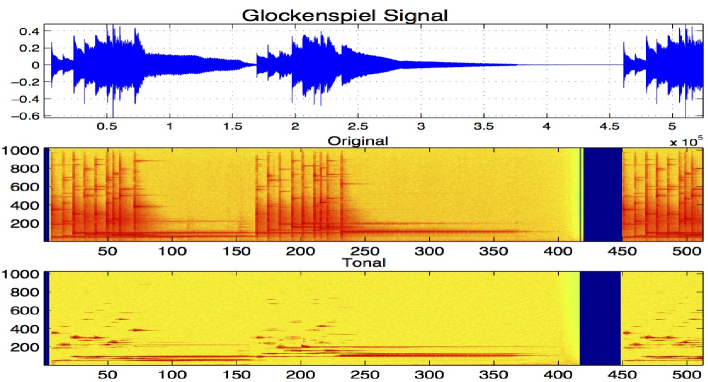
Figure 1. Estimating a tonal layer; top: glockenspiel signal; middle: logarithm of absolute value of MDCT coefficients of the signal; bottom: logarithm of absolute value of MDCT coefficients of a tonal layer, estimated using “horizontal” structures in MDCT coefficients.

In the framework of the recursive estimation scheme we are about to describe, the simplest (and natural) idea would be to start by expanding the signal with respect to a local cosine basis, and pick the largest coefficients (in absolute value, after appropriate weighting if needed) to form a best $N$-term approximation [7]. However, as may be seen in the middle image of Figure 1, such a strategy would automatically “capture” local cosine coefficients which definitely belong to transients (i.e. seem to form localized, “vertical” structures.) In order to avoid capturing such undesired coefficients, it is also natural to use the “structure” of MDCT coefficients of tonals, i.e. the fact that they have a tendancy to form “horizontal ridges”. This is the purpose of the tonal model described below. In the glockenspiel example of Figure 1, such a strategy produces a tonal layer whose MDCT is exhibited in the bottom image, from which it is easily seen that only “horizontally structured” coefficients have been retained.

2.1. Model and consequences

In the framework of the recursive approach, the signal is modeled as a structured harmonic mixture of Gaussians, i.e. expanded into an MDCT basis, with given cutoff frequency $N$

(9) $$x=\sum_{n=0}^{N-1}\sum_{k}Y_{kn}w_{kn}\ ,$$

where the coefficients of the expansion are (real, continuous) random variables $Y_{kn}$ whose distribution is governed by a family of “fixed frequency” Hidden Markov chains (HMC) $X_{kn},k=1,\dots$. According to the usual practice, we shall denote by $Y_{1:k,n}$ (resp. $X_{1:k,n}$) the random vector $(Y_{1n},\dots Y_{kn})$ (resp. $(X_{1n},\dots X_{kn})$), and use a similar notation for the corresponding values $(y_{1n},\dots y_{kn})$ (resp. $(x_{1n},\dots x_{kn})$.) $\rho_{Y_{1:k,n}}$ and $\rho_{Y_{k}}$ will denote the joint density of $Y_{1:k,n}$ and the density of $Y_{kn}$ respectively, and the density of $Y_{kn}$ conditioned by $X_{kn}$, assumed to be independent of $k$, will be denoted by

$$\psi_{n}(y|x)=\rho_{Y_{kn}}(y|X_{kn}=x)\ ,\quad x=T,N\ .$$

To be more precise, the model is characterized as follows:

1. For all $n$, $X_{\cdot n}$ is a Markov chain with state space

   $${\mathcal{X}}=\left\{T,R\right\}$$

   (“tonal” and “residual”, or non-tonal) and transition matrix ${\tilde{P}}_{n}$, of the form

   $${\tilde{P}}_{n}=\begin{pmatrix}{\tilde{\pi}}_{n}&1-{\tilde{\pi}}_{n}\\ 1-{\tilde{\pi}}_{n}^{\prime}&{\tilde{\pi}}_{n}^{\prime}\end{pmatrix}$$

   the numbers ${\tilde{\pi}}_{n},{\tilde{\pi}}_{n}^{\prime}$ being the persistence probabilities of the tonal and residual states: for all $n$

   (10) $${\tilde{\pi}}_{n}={\mathbb{P}}\left\{X_{kn}=T|X_{k-1\,n}=T\right\}\ ,$$

   (11) $${\tilde{\pi}}_{n}^{\prime}={\mathbb{P}}\left\{X_{kn}=R|X_{k-1\,n}=R\right\}\ .$$

   The initial frequencies of $T$ and $R$ states will be denoted by $\nu_{n}$ and $1-\nu_{n}$ respectively. For the sake of simplicity, we shall generally assume that the initial frequencies coincide with the equilibrium frequencies of the chain:

   $$\nu_{n}^{(e)}=\frac{1-{\tilde{\pi}}_{n}^{\prime}}{2-{\tilde{\pi}}_{n}-{\tilde{\pi}}_{n}^{\prime}}\ ,$$

2. The (emitted) coefficients $Y_{kn}$ are continuous random variables, with densities denoted by $\rho_{Y_{1:k\,n}}(y_{1:k\,n})$,

3. The distribution of the (emitted) coefficients $Y_{kn}$ depends only on the corresponding hidden state $X_{kn}$; for each $n$, the coefficients $Y_{kn}$ are independent conditional to the hidden states, and their distribution do not depend on the time index $k$ (but does depend on the frequency index $n$.) We therefore denote

   $$\rho_{Y_{1:kn}}\left(y_{1:kn}|X_{1:kn}=x_{1:kn}\right)=\prod_{i=1}^{k}\psi_{n}(y_{in}|x_{in})\ ,$$

4. In order to model audio signal, we shall limit ourselves to centered gaussian models for the densities $\psi_{k}$. The latter are therefore completely determined by their variances: a large variance $\sigma_{T}^{2}$ for the $T$ type coefficients, and a small variance $\sigma_{R}^{2}$ for the $R$ type coefficients.

Therefore, the model is completely characterized by the parameter set

$${\tilde{\theta}}=\{{\tilde{\pi}}_{n},{\tilde{\pi}}_{n}^{\prime};\nu_{n};{\tilde{\sigma}}_{T,n},{\tilde{\sigma}}_{R,n};\,n=0,\dots N-1\}\ .$$

Given these parameters, one may compute explicitly the likelihood of any configuration of coefficients. Using “routine” HMC techniques, it is also possible to obtain explicit formulas for the likelihood of any hidden states configuration, conditional to the coefficients. We refer to [24] for a detailed account of these aspects.

Remark 1.

Notice that in this version of the model, the transition matrix ${\tilde{P}}$ is assumed to be frequency independent. More general models involving frequency dependent ${\tilde{P}}$ matrices (or further generalizations) may be constructed, without much modifications of the overall approach.

Given a signal model as above, we may define the tonal layer of such a signal.

Definition 1.

Let $x$ be signal modeled as a hidden Markov chain MDCT as above, and let

(12) $$\Delta=\left\{(k,n)|X_{kn}=T\right\}\ .$$

$\Delta$ is called the tonal significance map of $x$. Then the tonal and non tonal layers are given by

(13) $$x_{ton} = \sum_{\delta\in\Delta}\beta_{\delta}w_{\delta}\ ,$$

(14) $$x_{nton} = x-x_{ton}$$

This definition makes it possible to obtain simple estimates for quantities of interest, such as the energy of a tonal signal, or the number of MDCT coefficients needed to encode it. For example, considering a time frame of $K$ consecutive windows (starting from $k=0$ for simplicity), and a frequency domain $\{0,\dots N-1\}$, we set

$$\Delta_{(K,N)}=\Delta\cap\left(\{0,\dots K-1\}\times\{0,\dots N-1\}\right)\ ,$$

and we denote by

(15) $$\tilde{N}_{n}^{(K)} = |\Delta_{(K,\{n\})}|$$

(16) $$\tau_{n}^{(K)} = {{\mathbb{E}}\left\{\frac{\tilde{N}_{n}^{(K)}}{K}\right\}}$$

the random variables describing respectively the number and the expected proportion of $T$ type coefficients in the frequency bin $n$, within a time frame of $K$ consecutive windows.

Proposition 1.

With the notations of Definition 1, the average proportion of $T$ type coefficients within the time frame $\{0,\dots K-1\}$ in the frequency bin $n$ is given by

(17) $$\tau_{n}^{(K)}=\frac{1}{K(2-{\tilde{\pi}}_{n}-{\tilde{\pi}}_{n}^{\prime})}\left[\nu_{n}((\!{\tilde{\pi}}_{n}\!+\!{\tilde{\pi}}_{n}^{\prime}\!-\!1\!)^{K}\!)\!+\!(\!1\!-\!{\tilde{\pi}}_{n}^{\prime}\!)\left(K-\frac{1\!-\!(\!{\tilde{\pi}}_{n}\!+\!{\tilde{\pi}}_{n}^{\prime}\!-\!1\!)^{K}}{2\!-\!{\tilde{\pi}}_{n}\!-\!{\tilde{\pi}}_{n}^{\prime}}\right)\right]$$

Proof: From classical properties of HMC, we have that

$$\begin{pmatrix}{\mathbb{P}}\left\{X_{k\,n}=T\right\}\\ {\mathbb{P}}\left\{X_{k\,n}=R\right\}\end{pmatrix}=\left({\tilde{P}}^{t}\right)^{k}\begin{pmatrix}\nu_{n}\\ 1-\nu_{n}\end{pmatrix}\ ,$$

the superscript “$t$” denoting matrix transposition. After some algebra, we obtain the following expressions:

$${\mathbb{P}}\left\{X_{k\,n}=T\right\} = \frac{\left((1-{\tilde{\pi}}_{n})\nu_{n}-(1-{\tilde{\pi}}_{n}^{\prime})(1-\nu_{n})\right)\left({\tilde{\pi}}_{n}+{\tilde{\pi}}_{n}^{\prime}-1\right)^{k}+(1-{\tilde{\pi}}_{n}^{\prime})}{2-{\tilde{\pi}}_{n}-{\tilde{\pi}}_{n}^{\prime}}$$

$$= \nu_{n}\left({\tilde{\pi}}_{n}+{\tilde{\pi}}_{n}^{\prime}-1\right)^{k}+\frac{1-{\tilde{\pi}}_{n}^{\prime}}{2-{\tilde{\pi}}_{n}-{\tilde{\pi}}_{n}^{\prime}}\,\left(1-({\tilde{\pi}}_{n}+{\tilde{\pi}}_{n}^{\prime}-1)^{k}\right)\ .$$

Similarly, we obtain for ${\mathbb{P}}\left\{X_{k\,n}=R\right\}=1-{\mathbb{P}}\left\{X_{k\,n}=T\right\}$

$${\mathbb{P}}\left\{X_{k\,n}=R\right\}=(1-\nu_{n})\left({\tilde{\pi}}_{n}+{\tilde{\pi}}_{n}^{\prime}-1\right)^{k}+\frac{1-{\tilde{\pi}}_{n}}{2-{\tilde{\pi}}_{n}-{\tilde{\pi}}_{n}^{\prime}}\,\left(1-({\tilde{\pi}}_{n}+{\tilde{\pi}}_{n}^{\prime}-1)^{k}\right)\ .$$

Finally, the result is obtained by replacing ${\mathbb{P}}\left\{X_{k\,n}=T\right\}$ with its expression in

$${{\mathbb{E}}\left\{\tilde{N}^{(K)}_{n}\right\}}=\sum_{k=0}^{K-1}{\mathbb{P}}\left\{X_{k\,n}=T\right\}\ ,$$

which yields the desired expression. ∎

Notice that in the limit of large time frames, one obtains the simpler estimate

$$\lim_{K\to\infty}\tau_{n}^{(K)}=\frac{1-{\tilde{\pi}}_{n}^{\prime}}{2-{\tilde{\pi}}_{n}-{\tilde{\pi}}_{n}^{\prime}}=\nu_{n}^{(e)}\ ,$$

which of course does not depend any more on $K$.

The energy of the tonal layer is also completely characterized by the parameters of the model, and has a simple behavior.

Proposition 2.

With the same notations as before, conditional to the parameters of the model, we have

(18) $$\begin{split}{{\mathbb{E}}\left\{\frac{1}{K}\sum_{\delta\in\Delta_{(K,N)}}|Y_{\delta}|^{2}\right\}}=&\frac{1}{K}\sum_{n=0}^{N-1}\frac{1}{2-{\tilde{\pi}}_{n}-{\tilde{\pi}}_{n}^{\prime}}\bigg{[}\left(1-({\tilde{\pi}}_{n}+{\tilde{\pi}}_{n}^{\prime}-1)^{K}\right)\nu_{n}{\tilde{\sigma}}_{T,n}^{2}\\ &\quad+(1-{\tilde{\pi}}_{n}^{\prime})\left(K-\frac{1-({\tilde{\pi}}_{n}+{\tilde{\pi}}_{n}^{\prime}-1)^{K}}{2-{\tilde{\pi}}_{n}-{\tilde{\pi}}_{n}^{\prime}}\right){\tilde{\sigma}}_{T,n}^{2}\bigg{]}\end{split}$$

Proof: the result follows from the fact that conditional to the hidden states, the considered random variables at fixed frequency are i.i.d. ${\mathcal{N}}(0,\sigma_{T,n}^{2})$ random variables. It is then enough to plug the expression of $\tau_{n}^{(K)}$ obtained above in the $L^{2}$ norm of the tonal layer.∎

Again, the latter expression simplifies in the limit $K\to\infty$, or if the initial frequencies of the chains $X_{n}$ are assumed to equal the equilibrium frequencies. In that situation, we obtain

(19) $$\lim_{K\to\infty}{{\mathbb{E}}\left\{\frac{1}{K}\sum_{\delta\in\Delta_{(K,N)}}|Y_{\delta}|^{2}\right\}}=\sum_{n=0}^{N-1}\frac{1-{\tilde{\pi}}_{n}^{\prime}}{2-{\tilde{\pi}}_{n}-{\tilde{\pi}}_{n}^{\prime}}\,{\tilde{\sigma}}_{T,n}^{2}=\sum_{n=0}^{N-1}\nu_{n}^{(e)}\,{\tilde{\sigma}}_{T,n}^{2}\ .$$

Remark 2.

Thanks to the simplicity of the Gaussian model, similar estimates may be obtained for other $\ell^{p}$-type norms.

A fundamental aspect of transform coding schemes based on non-linear approximations such as the one we are describing here is the fact that the significance maps $\Delta$ have to be encoded together with the corresponding coefficients. Since the significance map takes the form of a series of segments of $T$s and segments of $R$s with various lengths, it is natural to use classical techniques of run length coding (see for example [15], Chapter 10, for a detailed account) to encode them. The corresponding bit rate depends crucially on the entropy of the distribution of $T$ and $R$ segments. For the sake of simplicity, let us introduce the entropy of a binary source with probabilities $(p,1-p)$:

(20) $$h(p)=-p\log_{2}(p)-(1-p)\log_{2}(1-p)\ .$$

Proposition 3.

Assume that the initial frequencies of the chains $X_{\cdot n}$ equal their equilibrium frequencies. For each frequency bin $n$, the entropy of the distribution of lengths $L_{n}$ of $T$ and $R$ segments reads

(21) $${\mathcal{H}}(L_{n})=\frac{1-{\tilde{\pi}}_{n}^{\prime}}{2-{\tilde{\pi}}_{n}-{\tilde{\pi}}_{n}^{\prime}}h({\tilde{\pi}}_{n})+\frac{1-{\tilde{\pi}}_{n}}{2-{\tilde{\pi}}_{n}-{\tilde{\pi}}_{n}^{\prime}}h({\tilde{\pi}}_{n}^{\prime})\ .$$

Proof: Denote by $L_{T}$ and $L_{R}$ the lengths of $T$ and $R$ segments. From the Markov model $X$ it follows that $L_{T}$ and $L_{R}$ are exponentially distributed:

$${\mathbb{P}}\left\{L_{T}=\ell\right\}={\tilde{\pi}}_{n}^{\ell-1}(1-{\tilde{\pi}}_{n})\ ,\quad{\mathbb{P}}\left\{L_{R}=\ell\right\}={\tilde{\pi}}_{n}^{\prime\ell-1}(1-{\tilde{\pi}}_{n}^{\prime})\ ,\quad\ell=1,2,\dots$$

A simple calculation shows that the Shannon entropy of the random variable $L_{T}$ is given by

$$-\sum_{\ell=1}^{\infty}{\mathbb{P}}\left\{L_{T}=\ell\right\}\log_{2}\left({\mathbb{P}}\left\{L_{T}=\ell\right\}\right)=-{\tilde{\pi}}_{n}\log_{2}({\tilde{\pi}}_{n})-(1-{\tilde{\pi}}_{n})\log_{2}(1-{\tilde{\pi}}_{n})=h({\tilde{\pi}}_{n})\ ,$$

and a similar expression for the Shannon entropy of $L_{R}$. Now, because of the assumption on the initial frequencies of the chains $X_{\cdot n}$, and dropping the indices for the sake of simplicity, we have that

$${\mathbb{P}}\left\{X=T\right\}=\frac{1-{\tilde{\pi}}^{\prime}}{2-{\tilde{\pi}}-{\tilde{\pi}}^{\prime}}\ ,$$

and the equality

$${\mathcal{H}}(L)={\mathbb{P}}\left\{X=T\right\}{\mathcal{H}}(L_{T})+{\mathbb{P}}\left\{X=R\right\}{\mathcal{H}}(L_{R})$$

yields the desired result. ∎

Finally, let us briefly discuss questions regarding the quantization of coefficients. The simplicity of the model (Gaussian coefficients, and Markov chain significance map) makes it possible to obtain elementary rate-distortion estimates. Indeed, the optimal rate-distortion function for Gaussians random variables is well known: for a ${\mathcal{N}}(0,\sigma^{2})$ random variable,

(22) $$D(R)=\sigma^{2}\,2^{-2R}\ .$$

Let us assume that the $T$ type coefficients at frequency $n$ are quantized using $R_{n}$ bits per coefficient. Using the optimal rate-distortion function (22), the overall distortion per time frame is given by

$$D=\sum_{n=0}^{N-1}\frac{\tilde{N}^{(K)}_{n}}{K}\,{\tilde{\sigma}}_{T,n}^{2}\,2^{-2R_{n}}\ .$$

If we are given a global budget of $\overline{R}$ bits per sample, the optimal bit rate distribution over frequency bins is obtained by minimizing ${{\mathbb{E}}\left\{D\right\}}$ with respect to $R_{n}$, under the “global bit budget” constraint

$${{\mathbb{E}}\left\{\sum_{n=0}^{N-1}\frac{\tilde{N}^{(K)}_{n}}{K}\,R_{n}\right\}}=N\overline{R}\ ,$$

the expectation being taken with respect to the significance map $\Delta$. Assuming for the sake of simplicity that the Markov chain is at equilibrium (i.e. $\nu_{n}=\nu_{n}^{(e)}$ for all $n$), this yields the following simple expression

(23) $$R_{n}=\frac{N}{\overline{N}}\overline{R}+\frac{1}{2}\log_{2}({\tilde{\sigma}}_{T,n}^{2})-\frac{1}{2\overline{N}}\sum_{m=0}^{N-1}\nu_{m}^{(e)}\,\log_{2}({\tilde{\sigma}}_{m}^{2})\ ,$$

where we have denoted by

$$\overline{N}=\sum_{n=0}^{N-1}\nu_{n}^{(e)}$$

the average number of $T$ type coefficients per time frame. As usual in this type of calculation, the so-obtained optimal value of $R_{n}$ is generally not an integer number, and an additional rounding operation is needed in practice. The distortion obtained with the rounded bit rates is therefore larger than the bound obtained with the values above. Summarizing this calculation, and plugging these optimal bit rates into the expression of the distortion, we obtain

Proposition 4.

With the above notations, the following rate-distortion bound holds: for a given overall bit budget of $\overline{R}$ bits per $T$ type coefficient,

(24) $${{\mathbb{E}}\left\{D\right\}}\geq\overline{N}\,\left(\prod_{n=0}^{N-1}{\tilde{\sigma}}_{n}^{2\nu_{n}^{(e)}}\right)^{1/\overline{N}}\,2^{-2N\overline{R}/\overline{N}}\ .$$

2.2. Parameter and state estimation: algorithmic aspects

Hidden Markov models have been very successful because there exist naturally associated efficient algorithms for both parameter estimation and hidden state estimation, respectively the Expectation-Maximization (EM) and Viterbi algorithms. However, while these are natural answers to the estimation problems in general situations, they are not so natural anymore in a coding setting, as we explain below.

¿From a general point of view, an imput signal is first expanded with respect to an MDCT basis, corresponding to a fixed time segmentation (segments of approximately 20 msec.) Then, within larger time frames, the parameters are (re)estimated, as well as the hidden states. Parameters are refreshed on a regular basis.

2.2.1. Parameter estimation

Given the parameter set ${\tilde{\theta}}$ of the model, the forward-backward equations allow one to obtain estimates for the probabilities of hidden states conditional to the observations:

(25) $$p_{kn}(T) = {\mathbb{P}}\left\{X_{k\,n}=T|{\tilde{\theta}},Y_{1:K,n}=y_{1:K,n}\right\}\ ,$$

(26) $$p_{kn}(R) = {\mathbb{P}}\left\{X_{k\,n}=R|{\tilde{\theta}},Y_{1:K,n}=y_{1:K,n}\right\}$$

and the likelihood of the parameters

$${\mathcal{L}}({\tilde{\theta}})={\mathbb{P}}\left\{Y_{1:K,n}=y_{1:K,n}|{\tilde{\theta}}\right\}\ ,$$

from which new estimates for the parameter set ${\tilde{\theta}}$ may be derived.

Remark 3.

From a practical point of view, such parameter re-estimation happens to be quite costly. Therefore, the parameters are generally re-estimated on a larger time scale, taking several consecutive windows into account.

Remark 4.

For practical purpose, it is generally more suitable to restrict the parameter set ${\tilde{\theta}}$ to a smaller subset. The following two assumptions proved to be quite adapted to the case of audio signals:

• The variances may be assumed to be multiple of a single reference value, implementing some “natural” decay of MDCT coefficients with respect to frequency. For example, we generally used expressions of the form

  $${\tilde{\sigma}}_{s,n}=\frac{{\tilde{\sigma}}_{s}}{1+(\frac{n}{n_{0}})^{\alpha}},\quad s=T,R$$

  $n_{0}\in{\mathbb{R}}^{+}$ being some reference frequency bin, $\sigma_{s}$ a reference standard deviation for state $s$ and $\alpha\in{\mathbb{R}}^{+}$ some constant controlling the decay (typical value being $\alpha=1$). Without such an assumption, frequency bins are completely independent of each other, and the estimation algorithm generally yields $T$ type coefficients in all bins, which is not realistic,

• For each frequency bin, the initial frequencies $\nu_{n}$ of the considered Markov chain are generally assumed to equal the equilibrium frequencies $\nu_{n}^{(e)}$.

2.2.2. State estimation

Viterbi’s algorithm is generally considered the natural answer to the state estimation problem. It is a dynamic programing algorithm, which yields Maximum a posteriori (MAP) estimates

$$\hat{x}_{1:K\,n}=\arg\max{\mathbb{P}}\left\{X_{1:K\,n}=x_{1:K\,n}|y_{1:K\,n},{\tilde{\theta}}\right\}\ ,$$

for each frequency bin $n$. However, the number of so-obtained coefficients in a given state ($T$ or $R$) cannot be controlled a priori when such an algorithm is used, which turns out to be a severe limitation in a signal coding perspective. In addition, Viterbi’s algorithm requires that accurate estimates of the model’s parameters are available, which will not necessarily be the case if the parameter estimates are refreshed on a coarse time scale (see above.)

Therefore, we also consider, as an alternative to Viterbi’s algorithm, an a posteriori probabilities thresholding method, which is computationally far simpler, and allows a fine rate control. More precisely, given a prescribed rate $N_{ton}$,

• Sort the MDCT coefficients $y_{kn}=\langle x,w_{kn}\rangle$ in order of decreasing a posteriori probability $p_{kn}(T)$ in (25),

• Keep the $N_{ton}$ first sorted coefficients.

In this way, for an average bit rate $\overline{R}$ and a prescribed “tonal” bit budget, a number $N_{ton}$ of MDCT coefficients to be retained may be estimated, and the $N_{ton}$ coefficients with largest a posteriori probability are selected.

2.3. Numerical simulations

  

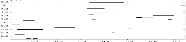
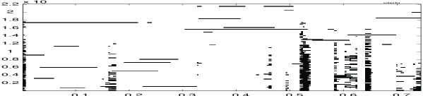
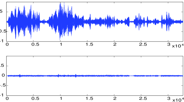
Figure 2. Estimating a tonal layer from simulated signal; from top to bottom: simulated significance map, estimated significance map (estimation via the Viterbi algorithm), estimated tonal signal, estimated residual signal.

As a first test of the model and the estimation algorithms, we generated realizations of the structured harmonic mixture of Gaussians model described above, and used the corresponding estimation algorithms. We simulated a signal according to the “tonal + residual” Markov model as above, with about 3.1% $T$-type coefficients. We show in Figure 2 the result of the estimation of the tonal layer using EM parameter estimation, and state estimation via the Viterbi algorithm. As may be seen, the significance map is fairly well estimated, except in regions where the signal has little energy, which was to be expected. In these regions, the algorithm detects spurious (vertical) tonal structures, which results in an increase of the percentage of $T$ type coefficients (about 4.1% instead of 3.2% for that example.) However, since this effect appears only in regions where the signal has small energy, this does not affect tremendously the estimated signal, which is very close to the simulated one (not shown here.)

For the sake of comparison, we display in Figures 3 and 4 some examples of tonal layer estimation using the thresholding algorithm instead of the Viterbi algorithm, for various values of the threshold. The simulation presented in Figure 3 corresponds to 1% retained coefficients, while the simulation presented in Figure 4 corresponds to 3% retained coefficients. As expected, the significance map in Figure 3 appears much terser than the “true” one, while the one in Figure 4 is much closer (percentage of retained coefficients significantly larger than the true one yield spurious tonal structures.) This results in tonal components which were not correctly captured, and appear in the residual signal of Figure 3. This is not the case any more when the threshold is set to a more “realistic” value, as may be seen in the tonal and residual layers of Figure 4. In that case, the residual only features a small spurious component. Notice that even though significantly less coefficients are retained, the overall shape of the estimated signal is quite good.

  

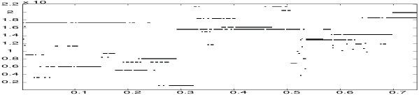
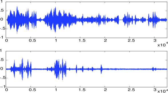
Figure 3. Estimating a tonal layer from simulated signal (same as in Figure 2); from top to bottom: estimated significance map (estimated via the posterior probability thresholding algorithm, using 1% coefficients); estimated tonal signal, estimated residual signal.

  

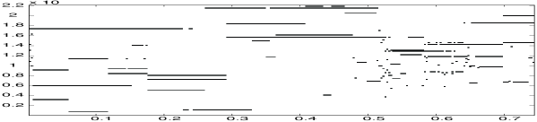
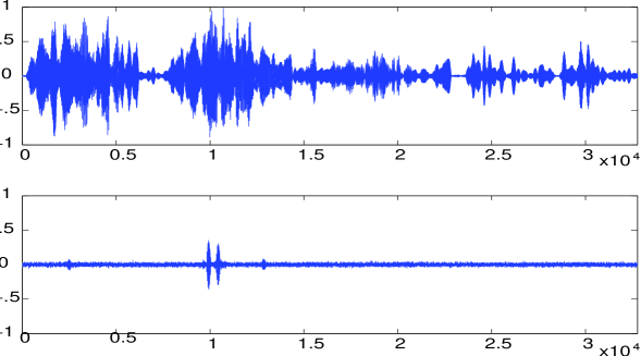
Figure 4. Estimating a tonal layer from simulated signal (same as in Figure 2); from top to bottom: estimated significance map (estimated via the posterior probability thresholding algorithm, using 3% coefficients); estimated tonal signal, estimated residual signal.

Remark 5.

Clearly, the posterior probability thresholding method only provides an approximation of the “true” tonal layer (which is provided by the Viterbi algorithm), whose precision depends on the choice of the threshold, i.e. the bit rate allocated to the tonal layer. Controlling the relation between the bit rate and the precision of the approximation would lead to a rate distortion theory for the “functional” part of the tonal coder. Such a theory seems extremely difficult to develop, and so far we could only study it by numerical simulations (not shown here.)

3. Structured Markov model for transient

3.1. Hidden wavelet Markov tree model

We now turn to the description of the transient model, which was partly presented in [21]. The latter exploits the fact that wavelet bases are “well adapted” for describing transients, in the sense that these generally yield scale-persistent chains of significant wavelet coefficients. We start from a multiresolution analysis (see for example [17, 29]) and the corresponding wavelet $\psi\in L^{2}({\mathbb{R}})$, scaling function $\phi\in L^{2}({\mathbb{R}})$ and wavelet basis, defined by

$$\psi_{jk}(t)=2^{-j/2}\,\psi\!\left(2^{-j}t-k\right)\ ,\quad j,k\in{\mathbb{Z}}\ .$$

Given $x\in L^{2}({\mathbb{R}})$, its wavelet coefficients $d_{jk}=\langle x,\psi_{jk}\rangle$ are naturally labelled by a dyadic tree, as in Figure 5, in which it clearly appears that a given wavelet coefficient $d_{jk}$ may be given a pair of children $d_{j+1\ 2k}$ and $d_{j+1\ 2k+1}$. For the sake of simplicity, we shall sometimes collect the two indices $j,k$ into the scale-time index $\lambda=(j,k)$.

For the sake of simplicity, we consider a fixed time interval, and a signal model involving finitely many scales, of the form

(27) $$x=S_{J0}\phi_{J0}+\sum_{j=1}^{J}\sum_{k=0}^{2^{J-j}-1}D_{jk}\psi_{jk}\ ,$$

involving

$$N(J)=2^{J}-1$$

random wavelet coefficients, whose distribution is a gaussian mixture governed by a hidden random variable.

Figure 5. Wavelet coefficients tree.

More precisely, distribution of the wavelet coefficients $D_{jk}$ depends on a hidden state $X_{jk}\in\{T,R\}$ ($T$ stands for “transient”, and $R$ for “residual”.) At each scale $j$, the $T$-type coefficients are modelled by a centered normal distribution with (large) variance $\sigma_{T,j}^{2}$. The $R$-type coefficients are modelled by a centered normal distribution with (small) variance $\sigma_{R,j}^{2}$.

The distribution of hidden states is given by a “coarse to fine” Markov chain, characterized by a $2\times 2$ transition matrix, and the distribution of the coarsest scale state. In order to retain only connected trees, we impose a taboo transition: the transition $R\to T$ is forbidden. Therefore, the transition matrix assumes the form

$$P_{j}=\left(\begin{array}[]{cc}\pi_{j}&1-\pi_{j}\\ 0&1\end{array}\right)$$

where $\pi_{j}$ denotes the scale persistence probability, namely the probability of transition $T\to T$ at scale $j$:

$$\pi_{j}={\mathbb{P}}\left\{X_{j-1,\ell}=T|X_{j,k}=T\right\}\ ,\ell=2k,2k+1\ .$$

The hidden Markov process is completely determined by the set of matrices $P_{j}$ and the “initial” probability distribution, namely the probabilities $\nu=(\nu_{T},\nu_{R})$ of states at the maximum considered scale $j=J$. The complete model is therefore characterized by the numbers $\pi_{j}$, $\nu$, and the emission probability densities:

$$\rho_{S}(d)=\rho(d|X=S)\ ,\quad S=T,R\ .$$

In the sequel, we shall always assume that the persistence probabilities are scale independent:

$$\pi_{i}=\pi\ ,\quad\forall i\ .$$

According to our choice (centered Gaussian distributions), the latter are completely characterized by their variances $\sigma_{T,j}^{2}$ and $\sigma_{R,j}^{2}$. All together, the model is completely specified by the parameter set

(28) $$\theta=\{\nu,\,\pi,\,\sigma_{T,j},\,\sigma_{R,j},\;j~{}=~{}1\dots J\}\ ,$$

which leads to the definition of transient significance map (termed transient feature in [21])

Definition 2.

Let the parameter set in (28) be fixed, and let $x$ denote a signal given by a hidden Markov tree model as in (27) above. Consider the random set

(29) $$\Lambda=\left\{(j,k),j=1,\dots j,\ k=0,\dots 2^{j}-1|X_{jk}=T\right\}\ .$$

$\Lambda$ is called the transient significance map of $x$. The corresponding transient layer of $x$ is defined as

(30) $$x_{tr}=\sum_{(j,k)\in\Lambda}D_{jk}\psi_{jk}\ .$$

From this definition, one may easily derive estimates on various coding rates. The key point is the following immediate remark. Let $N_{j}$ denote the number of $T$-type coefficients at scale $j$, and let

$$N=\sum_{j=1}^{J}N_{j}$$

the total number of $T$-type coefficients at scale $j$. The following result is fairly classical in branching processes theory (see for example [10, 16].)

Proposition 5.

Let $x$ denote a signal given by a hidden Markov tree model as in (27) above. Then the number $N$ of $T$ type coefficients is given by a Galton-Watson process. In particular, one has

(31) $${{\mathbb{E}}\left\{N_{j}\right\}}=\nu(2\pi)^{J-j}\ ,\quad\overline{N}:={{\mathbb{E}}\left\{N\right\}}=\nu\,\frac{(2\pi)^{J}-1}{2\pi-1}$$

(with the obvious modification for the case $\pi=1/2$.)

Therefore, it is obvious to obtain estimates for the energy of a transient layer:

Corollary 1.

The average energy of the transient layer of a signal $x$ reads

(32) $${{\mathbb{E}}\left\{\sum_{j,k;X_{jk}=T}|D_{jk}|^{2}\right\}}=\nu\sum_{j=1}^{j=J}\sigma_{j}^{2}(2\pi)^{J-j}\ .$$

Another simple consequence is the following a priori estimate for the cost of significance map encoding. It is known that it is possible to encode a binary tree at a cost which is linear in the number of nodes. We use the following strategy for encoding the tree $\Lambda$ (even though it is not optimal, it has the advantage of being simple. Improvements may be obtained by using entropy coding techniques, taking advantage of the probability distribution of trees, which is known as soon as the persistence probability $\pi$ is known.) We associate with each node of $\Lambda$ a pair of bits, set to 0 or 1 depending on whether the left and right children of the node belong to $\Lambda$ or not. Therefore, $R_{SM}$ is not larger than twice the number of nodes of $\Lambda$, i.e. the number of $T$-type coefficients. Therefore, we immediately deduce

Corollary 2.

Given the set of parameters $\theta$, and the corresponding Hidden Markov wavelet tree model, let $R_{SM}$ denote the number of bits necessary to encode the significance map of a transient wavelet coefficients tree, as above. Then we have

$${{\mathbb{E}}\left\{R_{SM}\right\}}\leq\left\{\begin{array}[]{ll}\displaystyle 2\nu\times\frac{1-(2\pi)^{J}}{1-2\pi}&\hbox{ if }\pi\neq 0.5,\\ 2\nu J&\hbox{ if }\pi=0.5.\end{array}\right.$$

The simplicity of the transient model (i.e. Galton-Watson significance map, and Gaussian $T$ coefficients) makes it possible to derive simple rate-distortion estimates, along lines similar to the ones we followed for the tonal layer. Assume that the $T$ type coefficients at scale $j$ are quantized using $R_{j}$ bits. Assuming (22), the overall distortion is given by

$$D=\sum_{j=1}^{J}N_{j}\sigma_{j}^{2}2^{-2R_{j}}\ .$$

Suppose we are given a global budget of $\overline{R}$ bits per sample. Minimizing ${{\mathbb{E}}\left\{D\right\}}$ with respect to $R_{j}$, under the “global bit budget” constraint

$${{\mathbb{E}}\left\{\sum_{j=1}^{J}N_{j}R_{j}\right\}}=N(J)\overline{R}$$

yields the following simple expression

(33) $$R_{j}=\frac{N(J)}{\overline{N}}\overline{R}+\frac{1}{2}\log_{2}(\sigma_{j}^{2})-\frac{1}{2}\frac{2\pi-1}{(2\pi)^{J}-1}\sum_{j=1}^{J}(2\pi)^{J-j}\,\log_{2}(\sigma_{j}^{2})\ .$$

Therefore, plugging this expression into the optimal rate-distortion function (22), we obtain the following rate-distortion estimate

Proposition 6.

With the same notations as before, we have the following estimate: for a given overall bit budget of $\overline{R}$ bits per $T$ type coefficient, the distortion is such that

(34) $${{\mathbb{E}}\left\{D\right\}}\geq\overline{N}\,\left(\prod_{j=1}^{J}\sigma_{j}^{2\overline{N_{j}}}\right)^{1/\overline{N}}\,2^{-2N(J)\overline{R}/\overline{N}}\ ,$$

where we have set

$$\overline{N_{j}}=\nu\,(2\pi)^{J-j}\ ,\quad\overline{N}=\nu\,\frac{(2\pi)^{J}-1}{2\pi-1}\ .$$

3.2. Parameters and state estimation

As in the case of the tonal layer, the parameter estimation and the hidden state estimation may be realized through standard EM and Viterbi type algorithms. These algorithms are mainly based upon adapted versions of the above mentioned forward-backward algorithm: the so-called “upward-downward” algorithm, proposed by Crouse and collaborators in [5]. Actually, we rather used a variant, the downward-upward algorithm, due to Durand and Gonçalves [11], which provides a better control of numerical accuracy of the computations. As a result, the algorithm provides estimates for quantities such as the hidden states probabilities

$${\mathbb{P}}\left\{X_{jk}=s\big{|}D_{1:2^{J}-1}=d_{1:2^{J}-1}1,\theta\right\}$$

and the likelihood

$${\mathcal{L}}=\rho_{D_{1:2^{J}-1}}\left(d_{1:2^{J}-1}\big{|}X_{{1:2^{J}-1}},\theta\right)\ .$$

3.2.1. Parameters estimation

The parameter estimation goes along lines similar to the ones outlined in Section 2.2.1 (see also [21] for additional details.) Again, since the parameter estimation procedure, involving upward-downward algorithm, is quite costly, it is done simultaneously on several consecutive time windows (i.e. several consecutive trees), and parameters are “refreshed” on larger time scales.

3.2.2. Hidden states estimation

Again, the situation is very similar to the situation encountered when dealing with the tonal layer. The “Viterbi-type” algorithm described in [11] theoretically provides an estimate for “the” transient significance map, and therefore the transient layer. However, it does not allow one to control the number of selected coefficients (the rate), and is therefore not appropriate in a context of variable bit rate coder. Hence, we rather turn to the (also computationally simpler) alternative, using thresholding of a posteriori probabilities.

The upward-downward algorithm provides estimates for the probabilities

$$p_{jk}(T)={\mathbb{P}}\left\{X_{jk}=T\big{|}D_{1:2^{J}-1}=d_{1:2^{J}-1},\theta\right\}\ .$$

Therefore, the corresponding tree nodes may be sorted according to the latter (in decreasing order.) For a given transient bit budget, a maximal number of nodes to be retained $N_{tr}$ may be estimated, and the nodes with largest “transientness” probability $p_{jk}(T)$ are selected, and the corresponding transient layer is reconstructed.

3.3. Numerical simulations

As for the case of the tonal layer, it is easy to perform numerical simulations of the model to evaluate the performances of the estimation algorithms. We display in Figure 6 the results of such simulations, using EM algorithm for parameter estimation, and the Viterbi algorithm for hidden states estimation. As may be seen from the plots, the significance tree and the transient layer are quite well estimated.

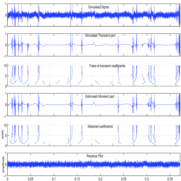
Figure 6. Estimating a transient layer from simulated signal; from top to bottom: simulated signal, simulated transient layer, simulated significance tree, estimated transient layer (estimation via the Viterbi algorithm), estimated significance tree, estimated residual signal.

Again, using the posterior probability thresholding method instead of the Viterbi method yields approximate transient layer, and the discussion of Remark 5 still hold true.

4. The “tonal vs transient” balance

We have described in Sections 2 and 3 two models for tonal and transient layers in audio signals, and corresponding estimation algorithms. One of the main aspects of the latter is that the hidden states estimation is based on thresholding of a posteriori probabilities rather than on a global Viterbi-type estimation, which allows to accomodate any bit rate prescribed in advance.

However, as stressed in the Introduction, and described in more detail in the subsequent section, we develop a coding approach based upon recursive estimations of tonal and transient layers. We describe below an approach for pre-estimating the relative sizes of the tonal and transient layers, in order to balance the bit budget between the two layers prior to estimation. The reader interested in more details is invited to refer to [22].

4.1. Pre-estimating the “sizes” of the tonal and transient layers

Consider a signal assumed for simplicity to be of the form (1), with unknown values of $|\Delta|$ and $|\Lambda|$, we seek estimates for the “transientness” and “tonality” indices

(35) $$I_{ton}=\frac{|\Delta|}{|\Delta|+|\Lambda|}\ ;\qquad I_{tr}=\frac{|\Lambda|}{|\Delta|+|\Lambda|}\ ,$$

or alternatively, the proportion of the signal’s energy contained in the tonal and transient layers. For simplicity, we limit ourselves to the finite dimensional situation, and propose a procedure very much in the spirit of the information theoretic approaches advocated by M.V. Wickerhauser and collaborators [27, 30].

Definition 3.

Let ${\mathcal{B}}=\{e_{n},n\in S\}$ be an orthonormal basis of a given $N$-dimensional signal space ${\mathcal{E}}$. The logarithmic dimension of $x\in{\mathcal{E}}$ in the basis ${\mathcal{B}}$ is defined by

(36) $${\mathcal{D}}_{\mathcal{B}}(x)=\frac{1}{N}\,\sum_{n\in S}\log_{2}\left(|\langle x,e_{n}\rangle|^{2}\ \right)$$

We aim to show that such quantity may provide the desired estimates, under suitable assumptions on the signal (sparsity) and the considered bases (incoherence.) Elementary calculations show that in the framework of the signal models (1), one has the following

Lemma 1.

Given an orthonormal basis ${\mathcal{B}}=\{e_{n},n\in S\}$, assuming that the coefficients $\langle x,e_{n}\rangle$ of $x\in{\mathcal{E}}$ are ${\mathcal{N}}(0,\sigma_{n}^{2})$ random variables, one has

(37) $${{\mathbb{E}}\left\{{\mathcal{D}}_{\mathcal{B}}(x)\right\}}=C+\frac{1}{N}\sum_{n\in S}\log_{2}(\sigma_{n}^{2})$$

where $C=1+\gamma/\ln(2)$ ($\gamma\approx.5772156649$ being Euler’s constant.)

Consider now the model (1), and assume that the coefficients $\alpha_{\lambda},\lambda\in\Lambda$ and $\beta_{\delta},\delta\in\Delta$ are respectively ${\mathcal{N}}(0,\sigma_{\lambda}^{2})$ and ${\mathcal{N}}(0,{\tilde{\sigma}}_{\delta}^{2})$ independent random variables. Then the coefficients

$$a_{\lambda}=\langle x,\psi_{\lambda}\rangle\ ;\quad b_{\delta}=\langle x,w_{\delta}\rangle\ ,$$

are centered normal random variables, whose variances depends on whether $\lambda\in\Lambda$ (or $\delta\in\Delta$) or not. For example, in the case of the $a_{\lambda}$ coefficients,

(38) $$\hbox{var}\{a_{\lambda}\}=\left\{\begin{array}[]{ll}\sigma_{\lambda}^{2}+\sum_{\delta\in\Delta}{\tilde{\sigma}}_{\delta}^{2}|\langle x,w_{\delta}\rangle|^{2}&\hbox{ if }\lambda\in\Lambda\\ \sum_{\delta\in\Delta}{\tilde{\sigma}}_{\delta}^{2}|\langle x,w_{\delta}\rangle|^{2}&\hbox{ if }\lambda\not\in\Lambda\ ,\\ \end{array}\right.$$

which yields

(39) $${{\mathbb{E}}\left\{{\mathcal{D}}_{\Psi}(x)\right\}}=C+\frac{1}{N}\log_{2}\!\!\left(\prod_{\lambda\in\Lambda}\!\!\left(\sigma_{\lambda}^{2}+\!\!\sum_{\delta\in\Delta}{\tilde{\sigma}}_{\delta}^{2}|\langle\psi_{\lambda},w_{\delta}\rangle|^{2}\right)\prod_{\lambda^{\prime}\not\in\Lambda}\!\!\left(\sum_{\delta\in\Delta}{\tilde{\sigma}}_{\delta}^{2}|\langle\psi_{\lambda^{\prime}},w_{\delta}\rangle|^{2}\right)\right)\ ,$$

and a similar expression for the logarithmic dimension ${\mathcal{D}}_{W}(x)$ with respect to the $W=\{w_{\delta}\}$ basis.

For the sake of simplicity, we now assume that $\sigma_{\lambda}=\sigma$, $\forall\lambda\in\Lambda$ and ${\tilde{\sigma}}_{\delta}={\tilde{\sigma}}$, $\forall\delta\in\Delta$. Introduce the Parseval weights

(40) $$p_{\lambda}(\Delta)=\sum_{\delta\in\Delta}|\langle w_{\delta},\psi_{\lambda}\rangle|^{2}\ ,\quad{\tilde{p}}_{\delta}(\Lambda)=\sum_{\lambda\in\Lambda}|\langle w_{\delta},\psi_{\lambda}\rangle|^{2}\ .$$

The Parseval weights provide information regarding the “dissimilarity” of the two considered bases. The following property is a direct consequence of Parseval’s formula:

Lemma 2.

With the above notations, the Parseval weights satisfy

$$0\leq p_{\lambda}(\Delta)\leq 1\ ,\quad 0\leq{\tilde{p}}_{\delta}(\Lambda)\leq 1\ .$$

Introduce the relative redundancies of the bases $\Psi$ and $W$ with respect to the significance maps

(41) $$\epsilon(\Delta)=\max_{\lambda\in\Lambda}p_{\lambda}(\Delta)\ ,\quad{\tilde{\epsilon}}(\Lambda)=\max_{\delta\in\Delta}p_{\delta}(\Lambda)\ .$$

These quantities carry information similar to the one carried by the Babel function used in [28] for example. One then obtains simple estimates for the logarithmic dimension [22].

Proposition 7.

With the above notations, assuming that the significant coefficients $\alpha_{\lambda},\lambda\in\Lambda$ and $\beta_{\delta},\delta\in\Delta$ are i.i.d. ${\mathcal{N}}(0,\sigma^{2})$ and ${\mathcal{N}}(0,{\tilde{\sigma}}^{2})$ normal variables respectively, one has the following bound

(42) $$\quad{{\mathbb{E}}\left\{{\mathcal{D}}_{\Psi}(x)\right\}} \geq C+\frac{|\Lambda|}{N}\log_{2}(\sigma^{2})+\log_{2}\left(\prod_{\lambda^{\prime}\not\in\Lambda}\!\left({\tilde{\sigma}}^{2}p_{\lambda^{\prime}}(\Delta)\right)^{1/N}\right)$$

(43) $$\quad{{\mathbb{E}}\left\{{\mathcal{D}}_{\Psi}(x)\right\}} \leq C+\frac{|\Lambda|}{N}\log_{2}(\sigma^{2}+\epsilon(\Delta){\tilde{\sigma}}^{2})+\log_{2}\left(\prod_{\lambda^{\prime}\not\in\Lambda}\!\left({\tilde{\sigma}}^{2}p_{\lambda^{\prime}}(\Delta)\right)^{1/N}\right)\ .$$

Exchanging the roles of $\Delta$ and $\Lambda$, a similar bound is obtained for ${\mathcal{D}}_{W}(x)$.

At this point, several comments have to be made.

• The bounds in Equations (42) and (43) differ by $|\Lambda|\log_{2}(1+\epsilon(\Delta){\tilde{\sigma}}^{2}/\sigma^{2})/N$. Let us temporarily assume that this term may be neglected (see comment b. below for more details.) The behavior of ${{\mathbb{E}}\left\{{\mathcal{D}}_{\Psi}(x)\right\}}$ is therefore essentially controlled by

  $$\log_{2}\left(\prod_{\lambda^{\prime}\not\in\Lambda}\!\left({\tilde{\sigma}}^{2}p_{\lambda^{\prime}}(\Delta)\right)^{1/N}\right)$$

  Such an expression is not easily understood, but a first idea may be obtained by replacing $p_{\lambda^{\prime}}(\Delta)$ by its “ensemble average”

  $$\frac{1}{N}\sum_{\lambda=1}^{N}p_{\lambda}(\Delta)=\frac{1}{N}\sum_{\lambda=1}^{N}\sum_{\delta\in\Delta}|\langle w_{\delta},\psi_{\lambda}\rangle|^{2}=\frac{1}{N}\sum_{\delta\in\Delta}\|w_{\delta}\|^{2}=\frac{|\Delta|}{N}\ ,$$

  which yields the approximate expression:

  (44) $${{\mathbb{E}}\left\{{\mathcal{D}}_{\Psi}(x)\right\}}\approx C+\frac{|\Lambda|}{N}\log_{2}(\sigma^{2})+\left(1-\frac{|\Lambda|}{N}\right)\,\log_{2}\left({\tilde{\sigma}}^{2}\frac{|\Delta|}{N}\right)\ .$$

  Therefore, if the “$\Psi$-component” of the signal is sparse enough, i.e. if $|\Lambda|/N$ is sufficiently small (compared with 1), ${{\mathbb{E}}\left\{{\mathcal{D}}_{\Psi}(x)\right\}}$ may be expected to behave as $\log_{2}\left({\tilde{\sigma}}^{2}\frac{|\Delta|}{N}\right)$, which suggests to use

  (45) $$\hat{N}_{\psi}(x)=2^{{\mathcal{D}}_{\Psi}(x)}$$

  as an estimate (up to a multiplicative constant) for the “size” of the $W$ component of the signal. Notice that this expression coincides with (2),

• The difference between the lower and upper bounds depends on two parameters: the sparsity $|\Lambda|/N$ of the $\Psi$-component, and the relative redundancy parameters $\epsilon(\Delta)$. The latter actually describe the intrinsic differences between the two considered bases. When the bases are significantly different, the relative redundancy may be expected to be small (notice that in any case, it is smaller than 1),

• The relative redundancy parameters $\epsilon$ and ${\tilde{\epsilon}}$ which pop up in our model differs from the one which is generally considered in the literature, namely the coherence of the dictionary $W\cup\Psi$ (see e.g. [9, 12, 14])

  $$\mu[W\cup\Psi]=\sup_{\stackrel{{\scriptstyle b,b^{\prime}\in W\cup\Psi}}{{b\neq b^{\prime}}}}|\langle b,b^{\prime}\rangle|\ ,$$

  and the Babel function (see [28, 14].) The latter are intrinsic to the dictionary, while the Parseval weights and corresponding $\epsilon$ and ${\tilde{\epsilon}}$ provide a finer information, as they also account for the signal models, via their dependence in the significance maps $\Lambda$ and $\Delta$,

• Precise estimates for $\epsilon$ and ${\tilde{\epsilon}}$ are fairly difficult to obtain. What would actually be needed is a tractable model for the significance maps $\Delta$ and $\Lambda$, in the spirit of the structured models described in the two previous sections (for which we couldn’t obtain simple estimates.) Returning to the wavelet and MDCT case, it is quite natural to expect that models implementing time persistence in $\Delta$ and scale persistence in $\Lambda$ would yield smaller values for the relative redundancies than models featuring uniformly distributed significance maps.

A more detailed analysis of this method (including a discussion of noise robustness issues) is presented in [22].

4.2. Numerical simulations

The above discussion suggest to use the logarithmic dimensions in order to get estimates for the relative sizes of the tonal and transient layers in audio signals. We shall use the following estimated proportions

(46) $$\hat{I}_{ton}=\frac{\hat{N}_{\psi}}{\hat{N}_{\psi}+\hat{N}_{w}}\ ;\qquad\hat{I}_{tr}=\frac{\hat{N}_{w}}{\hat{N}_{\psi}+\hat{N}_{w}}\ ,$$

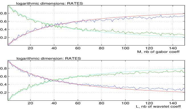
Figure 7. Simulations of tonality and transientness indices, as functions of $|\Delta|$ or $|\Lambda|$ (time frames of 1024 samples): theoretical curves and simulation (averaged over 10 realizations); top plot: $|\Lambda|=40$, varying $|\Delta|$, $I_{tr}$ (decreasing curve) and $I_{ton}$ (increasing curve); top plot: $|\Delta|=40$, varying $|\Lambda|$, $I_{ton}$ (decreasing curve) and $I_{tr}$ (increasing curve.)

In order to validate this approach, we computed these quantities on simulated signals of the form (1), as functions of $|\Delta|$ (resp. $|\Lambda|$) for fixed values of $|\Lambda|$ (resp. $|\Delta|$.) The result of such simulations is displayed in Figure 7, which show $\hat{I}_{ton}$ and $\hat{I}_{tr}$ as functions of $|\Delta|$, together with the theoretical curves defined in (35), averaged over 20 realizations. As may be seen, the results are fairly satisfactory, which indicates that such indicator may be used for estimating the percentage of bit rate to be allowed to the different components, prior to the hybrid coding itself.

 

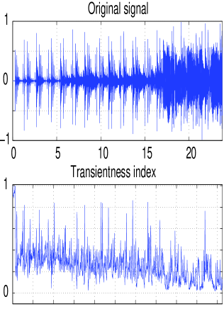
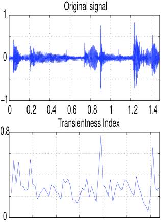
Figure 8. Tonal vs Transient balance for a real audio signal (a musical signal.) Left: long signal (about 23 seconds long): top plot: original signal; bottom plot: transientness index. Right: shorter (1.5 seconds long) segment, same legend.

An example on real audio signal is displayed in Figure 8, which represents the transientness index (from which the tonality index is easily deduced) for a segment (about 23 seconds) of audio signal (the mamavatu signal, which will be used again as illustration in the next section.) A shorter segment of 1.5 seconds (located in the middle of the large segment) is analyzed similarly in the right hand plots of Figure 8 As may be seen, the transientness index (lower curves) exhibits significant local maxima in the neighborhood of the various “attacks” of the signal (see the left hand plots of Figure 8.) Notice also on the right hand plots of Figure 8 that the transientness index exhibits an overall decay in the rightmost part of the plot. This is mainly due to the fact that a significant tonal component shows up in that part of the signal (see Figure 10 in the next section), which reduces the proportion of transients (we recall that the transientness index really measures the proportion, and not the quantity of transient signal present.)

Remark 6.

It is worth noticing that the indices $\hat{I}_{ton}$ and $\hat{I}_{tr}$ perform satisfactorily as long as the two expansions in (1) are sparse enough. Otherwise, deviations from the “ideal” behavior have to be expected, as may be seen in the right hand side of the plots in Figure 7.

Remark 7.

Also, $\hat{I}_{ton}$ and $\hat{I}_{tr}$ provide estimates for the sizes of significance maps only when the variances $\sigma^{2}$ and ${\tilde{\sigma}}^{2}$ are of comparable magnitude. When this is not the case, it is easily seen that they rather provide estimates on the relative energies of the two layers, for example $\hat{I}_{tr}=|\Lambda|\sigma^{2}/(|\Lambda|\sigma^{2}+|\Delta|{\tilde{\sigma}}^{2})$. The behavior of the indices in noisy situations (i.e. with small, additive white noise) may be studied as well, and yields similar conclusions, as long as the noise’s energy is small enough [22].

5. Application to audio coding

The ideas developed above are currently being implemented within a prototype hybrid audio coder, extending the ideas already described in [7]. While the idea of hybrid coding of audio signals is not new, our approach is the first one that implements hybrid transform coding without prior (time) segmentation of the signal. A detailed account of the coding system will be given in a forthcoming publication, together with systematic performance evaluations. However, we find it interesting to sketch the main features here, as they provide a thorough applications of the probabilistic models we just described.

5.1. Description of a prototype coder

Figure 9. Block diagram of the hybrid audio coding scheme

The block diagram of the encoder is displayed in Figure 9 (the corresponding decoder simply amounts to invert MDCT and DWT transforms from the encoded coefficients). The first step of the algorithm is a pre-estimation of the relative sizes of the tonal and transient layers, according to the discussion of section 4. Hence, any given bit budget may be allocated a priori to the different layers of the signal.

The second step is the estimation of the (structured) tonal layer, according to section 2. The parameters of the hidden Markov models are estimated and updated on large time frames, and the hidden states are estimated by thresholding of a posteriori probability. This yields estimated tonal and non-tonal layers

$$x_{ton}=\sum_{\delta\in\Delta}\langle x,w_{\delta}\rangle w_{\delta}\ ;\quad x_{nton}=x-x_{ton}\ .$$

The tonal layer is then quantized and encoded using standard techniques (either uniform quantization, or Lloyd-Max quantization, for gaussian sources, followed by entropy coding), while the non tonal layer is transmitted to the transient layer estimator. Since the parameters of the model (i.e. the persistence probabilities) provide explicitly the probabilities of lengths of “tonal structures”, the corresponding Huffmann code is readily obtained, and used for encoding the significance map.

The third step is the estimation of the transient layer from the non-tonal component. Again, transform coding is computed within time frames of about 23 milliseconds. The parameters of the hidden Markov model are estimated, and updated on larger time frames. Hidden states (i.e. the significance map) are estimated within each (small) time frame by thresholding of a posteriori state probability. Once the transient layer $x_{tr}$ has been estimated, it is substracted from the signal to yield the residual; in parallel, the coefficients are quantized and entropy coded. The tree structure of the transient significance map make it possible to derive an efficient way of encoding it (see [21].)

$$x_{tr}=\sum_{\lambda\in\Lambda}\langle x_{nton},\psi_{\lambda}\rangle\psi_{\lambda}\ ;\quad x_{res}=x_{nton}-x_{tr}\ .$$

The residual is finally modeled as a (locally) stationary random process, and currently encoded as such using fairly classical LPC procedures (even though this might not be the optimal solution for very low bit rate; this subject is currently under study.)

Notice that while the encoding procedure is quite complex (involving fairly sophisticated estimation algorithms), the decoding is extremely simple. The tonal and transient layers are reconstructed on the basis of their significance maps and corresponding encoded coefficients. The residual is re-generated using LPC technique.

5.2. Numerical illustrations

An example of hybrid (or multilayered) signal expansion obtained using the technique described in this paper is shown in Figure 10 (see Figure 8 for the corresponding transientness index.) In that example 6% of coefficients were retained (no coefficient quantization was done, so this essentially represents only the “functional” part of the compression.)

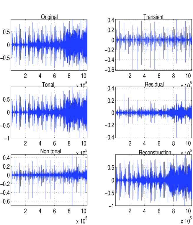
Figure 10. Compressed hybrid expansion of a piece of musics (mamavatu, about 23 seconds long.) From top to bottom, and from left to right: original signal, tonal layer, nontonal signal, transient layer, residual layer, and reconstruction from the three layers.

To demonstrate the ability of the proposed procedure to yield good signal approximations, we display in Figure 11 a comparison of Signal to Noise (SNR) curves for various encoding techniques, namely classical MDCT and DWT transform coding, as well as hybrid coding as proposed in [7] and the approach described in this paper. As may be seen, the performances of the different approaches are essentially comparable, the standard DWT and MDCT transform coding techniques (in the left curve) being better by a few dB. The N-term hybrid method appears to be slightly better than the Markov one. This is not really surprizing, as the SNR is computed from the $L^{2}$ distortion, and the introduction of structures in the approximation cannot improve the $L^{2}$ distortion in comparison with simple coefficient thresholding. Nevertheless, we notice that this effect is a very weak one.

For the same reason, introducing a normalization on MDCT coefficients prior to the selection (right-hand part of Figure 11) strongly penalizes the N-term MDCT method in terms of $L^{2}$ distortion. Interestingly enough, this does not seem to be the case for the two hybrid methods.

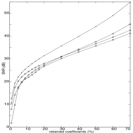
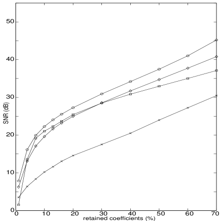
Figure 11. Comparison of “functional” Signal to Noise Ratios for various coding techniques, computed on the same test signal. Two configurations are represented: in the left-hand plot, coefficients were selected without prior normalization in the N-term MDCT (x), DWT ($\circ$) and hybrid ($\diamond$) methods, and $\alpha$ was equivalently set to 0 in the Markov method ($\square$, see Remark 4). In the right-hand plot, MDCT coefficients were normalized by a linear function of the frequency in the N-term MDCT and hybrid methods (no change in the wavelet method), and $\alpha$ was set to 1 in the Markov method.

One main outcome of the proposed method is that it provides a decomposition of the signal into several layers (two, or three if the residual is considered), i.e. one has to encode several signals instead of one. Nevertheless, Figure 11 (right) shows that in terms of SNR, this approach remains comparable with a standard DWT approximation scheme. In addition, the significance maps are encoded much more efficiently in the Markov approach (see Proposition 3 and Corollary 2).

Remark 8.

It is worth pointing out an important aspect of audio signal coding. It is well known that the $L^{2}$ distortion is not an adequate distortion measure for audio signals: it does not take into account the variation of the hearing threshold as a function of frequency (which could be done by an appropriate weighting of the $L^{2}$ norm in the frequency domain), nor the nonlinear masking effects, which are extremely important from the perceptual point of view (see for example [23] for a review). The natural distortion measure that introduces itself naturally in the present scheme is the likelihood, which takes into account the structures proposed in the model. For that reason, we believe that such a distortion measure is more “natural” from a perceptual point of view, though we do not have a clear evidence yet.

To illustrate the latter remark, the interested reader may find on the companion web site of this paper (see footnote 8) further illustrations of the behaviour of the proposed coding technique on real audio signals, as well as corresponding sound examples.

6. Conclusions and perspectives

This work was based on the belief that efficient signal modeling cannot be based solely on considerations on individual coefficients on a well chosen basis (even though one generally tries to use “bases that decorrelate”) and may be seen as an attempt to systematically exploit “structures”, or “persistence properties” in the coefficient domain. In this respect, the main contributions of this article are the new hybrid model we propose, and the a priori rate estimations which may be deduced from it, thanks to the relative simplicity of the model (First order Markov chains, and Gaussian distributions.)

We have specially emphasized in Section 5 the application to audio coding and compression. More details on the current implementation of the codec will be published elsewhere [6] together with a more complete analysis of quantization issues, and more detailed numerical results. Further developments involve designing coefficient quantization procedures specifically adapted to the tonal and transient layers, as well as the implementation of adapted masking methods (frequency masking and time masking.)

Finally, we would also like to point out that compression is far from being the only application of such models, and that coding is not limited to compression applications. An efficient coding scheme, such as the one we propose, should also prove useful for various applications such as automatic music transcription (exploiting the tonal layer) and onset detection (exploiting the transient layer). The multilayered signal representation could also simplify other audio processing tasks such as time-stretching, or various other signal modification problems, which may thus be performed directly in the coefficient domain. Among the other potential applications of such techniques, let us also mention blind source separation, which we plan to investigate in the future.

Acknowledgements. This work was supported in part by the European Union’s Human Potential Programme, under contract HPRN-CT-2002-00285 (HASSIP.) We also acknowledge support from the AMADEUS Austrian-French exchange programme, which allowed us to visit the NuHAG group in Vienna, where we had stimulating exchanges of ideas. We also wish to thank L. Daudet, F. Jaillet, Ph. Guillemain and R. Kronland-Martinet for many stimulating discussions.

References

- [1] J. Berger, R. Coifman, and M. Goldberg. Removing noise from music using local trigonometric bases and wavelet packets. J. Audio Eng. Soc., 42(10):808–818, 1994.
- [2] R. Carmona, W.L. Hwang, and B. Torrésani. Practical Time-Frequency Analysis: continuous wavelet and Gabor transforms, with an implementation in S, volume 9 of Wavelet Analysis and its Applications. Academic Press, San Diego, 1998.
- [3] S.S. Chen, D.L. Donoho, and M.A. Saunders. Atomic decomposition by basis pursuit. SIAM Journal on Scientific Computing, 20(1):33–61, 1998.
- [4] A. Cohen, W. Dahmen, I. Daubechies, and R. DeVore. Tree approximation and optimal encoding. Appl. Comput. Harmon. Anal., 11(2):192–226, 2001.
- [5] M. S. Crouse, R. D. Nowak, and R. G. Baraniuk. Wavelet-based signal processing using hidden Markov models. IEEE Transactions on Signal Processing, 46:886–902, april 1998. Special Issue on Filter Banks.
- [6] L. Daudet, S. Molla, and B. Torrésani. An Hybrid Structural Audio Coder. Technical report, Laboratoire d’Analyse, Topologie et Probabilités, Université de Provence, Marseille (France), 2003. In preparation.
- [7] L. Daudet and B. Torrésani. Hybrid representations for audiophonic signal encoding. Signal Processing, 82(11):1595–1617, 2002. Special issue on Image and Video Coding Beyond Standards.
- [8] N. Delprat, B. Escudié, P. Guillemain, R. Kronland-Martinet, P. Tchamitchian, and B. Torrésani. Asymptotic wavelet and gabor analysis: extraction of instantaneous frequencies. IEEE Trans. Inf. Th., 38:644–664, 1992. Special issue on Wavelet and Multiresolution Analysis.
- [9] D.L. Donoho and X. Huo. Uncertainty principles and ideal atomic decompositions. IEEE Trans. Inf. Th., 47(7):2845–2862, 2001.
- [10] J.L. Doob. Stochastic Processes. John Wiley & Sons, 1953.
- [11] J.B. Durand and P. Gonçalves. Statistical inférence for hidden markov tree models and application to wavelet trees. Technical Report 4248, Institut National de Recherches en Automatique et Informatique, September 2001.
- [12] M. Elad and A.M. Bruckstein. A generalized uncertainty principle and sparse representations. IEEE Trans. Inf. Th., 48(9):2558–2567, 2001.
- [13] R. Gribonval. Approximations non-linéaires pour l’analyse des signaux sonores. PhD thesis, Université de Paris IX Dauphine, 1999.
- [14] R. Gribonval and M. Nielsen. Sparse representations in union of bases. Technical Report 1499, Institut National de Recherches en Informatique et Automatique, IRISA Rennes, 2003.
- [15] N. S. Jayant and P. Noll. Digital coding of waveforms. Prentice-Hall, 1984.
- [16] S. Karlin. A first course on stochastic processes. Academic Press, Singapor, 1997. Second edition.
- [17] S. Mallat. A wavelet tour of signal processing. Academic Press, 1998.
- [18] S. Mallat and Z. Zhang. Matching pursuits with time-frequency dictionaries. IEEE Transactions on Signal Processing, 41:3397–3415, 1993.
- [19] R.J. McAulay and Th.F. Quatieri. Speech analysis/synthesis based on a sinusoidal representation. IEEE Trans. on Acoust., Speech and Signal Proc., 34:744–754, 1986.
- [20] F.G. Meyer, A.Z. Averbush, and R.R. Coifman. Multilayered image representation: Application to image compression. IEEE Transactions on Image Processing, 11:1072–1080, 2002.
- [21] S. Molla and B. Torrésani. Hidden markov trees of wavelet coefficients for transient detection in audiophonic signals. In A. Benassi, editor, Proceedings of the conference Self-Similarity and Applications, Clermont-Ferrand (May 2002), 2003. to appear.
- [22] S. Molla and B. Torrésani. Determining local transientness of audio signals. IEEE Signal Processing Letters, 11(7):625–628, July 2004.
- [23] T. Painter and A. Spanias. Perceptual coding of digital audio. Proc. IEEE, 88(4), april 2000.
- [24] L.R. Rabiner. A tutorial on hidden markov models and selected applications in speech recognition. Proceedings of the IEEE, 77:257–286, 1989.
- [25] A. Said and W. A. Pearlman. A new, fast, and efficient image codec based on set partitionning in hierarchical trees. IEEE Trans. on Circ. and Syst. for Video Tech, 6(3):243–250, 1996.
- [26] J. M. Shapiro. Embedded image coding using zerotrees of wavelet coefficients. IEEE Trans. Signal Processing, 41(12):3445–3462, 1993.
- [27] A. Trgo and M.V. Wickerhauser. A relation between Shannon–Weaver entropy and “theoretical dimension” for classes of smooth functions. Preprint, Washington University, Saint Louis, Missouri, 1995.
- [28] J.A. Tropp. Greed is good: Algorithmic results for sparse approximation. Technical report, Texas Institute of Computational and Applied Mathematics, 2002. available at http://www.math.princeton.edu/tfbb/spring03/greed-ticam0304.pdf.
- [29] M. Vetterli and J. Kovacevic. Wavelets and subband coding. Prentice Hall, Englewood Cliffs, NJ, USA, 1995.
- [30] M. V. Wickerhauser. Adapted Wavelet Analysis from Theory to Software. AK Peters, Boston, MA, USA, 1994.