Time-dependent complete-active-space self-consistent field method for multielectron dynamics in intense laser fields

Abstract

The time-dependent complete-active-space self-consistent-field (TD-CASSCF) method for the description of multielectron dynamics in intense laser fields is presented, and a comprehensive description of the method is given. It introduces the concept of frozen-core (to model tightly bound electrons with no response to the field), dynamical-core (to model electrons tightly bound but responding to the field), and active (fully correlated to describe ionizing electrons) orbital subspaces, allowing compact yet accurate representation of ionization dynamics in many-electron systems. The classification into the subspaces can be done flexibly, according to simulated physical situations and desired accuracy, and the multiconfiguration time-dependent Hartree-Fock (MCTDHF) approach is included as a special case. To assess its performance, we apply the TD-CASSCF method to the ionization dynamics of one-dimensional lithium hydride (LiH) and LiH dimer models, and confirm that the present method closely reproduces rigorous MCTDHF results if active orbital space is chosen large enough to include appreciably ionizing electrons. The TD-CASSCF method will open a way to the first-principle theoretical study of intense-field induced ultrafast phenomena in realistic atoms and molecules.

I introduction

The advent of the chirped pulse amplification (CPA) technique Strickland and Mourou (1985) has enabled the production of femtosecond laser pulses whose focused intensity easily exceeds $10^{14}\,{\rm W/cm}^{2}$ and even reach $\sim 10^{22}\,{\rm W/cm}^{2}$ Bahk et al. (2004); Yanovsky et al. (2008); Yu et al. (2012). Exposed to visible-to-mid-infrared pulses with an intensity typically higher than $10^{14}\,{\rm W/cm}^{2}$, atoms and molecules exhibit nonperturbative nonlinear response such as above-threshold ionization (ATI), tunneling ionization, high-order harmonic generation (HHG), and nonsequential double ionization (NSDI) Protopapas et al. (1997); Brabec and Krausz (2000). HHG, for example, represents a highly successful avenue toward an ultrashort coherent light source in the extreme-ultraviolet (XUV) and soft x-ray regions Seres et al. (2005); Chang (2011). The development of these novel light sources has opened new research possibilities including ultrafast molecular probing Itatani et al. (2004); Haessler et al. (2010); Salières et al. (2012), attosecond science Agostini and DiMauro (2004); Krausz and Ivanov (2009); Gallmann et al. (2013), and XUV nonlinear optics Sekikawa et al. (2004); Nabekawa et al. (2005).

In parallel with the progress in experimental techniques, various numerical methods have been developed to explore atomic and molecular dynamics in intense laser fields. While direct solution of the time-dependent Schrödinger equation (TDSE) provides exact description, this method is virtually unfeasible for multielectron systems beyond He Pindzola and Robicheaux (1998a, b); Colgan et al. (2001); Parker et al. (2001); Laulan and Bachau (2003); Piraux et al. (2003); Laulan and Bachau (2004); Ishikawa and Midorikawa (2005); Feist et al. (2009); Pazourek et al. (2011); Ishikawa and Ueda (2012); Sukiasyan et al. (2012); Ishikawa and Ueda (2013) and ${\rm H}_{2}$ Vanroose et al. (2006); Horner et al. (2008); Lee et al. (2010). As a result, single-active electron (SAE) approximation is widely used, in which only the outermost electron is explicitly treated, and the effect of the others, assumed to be frozen, is embedded in a model potential. This approximation, however, fails to account for multielectron and multichannel effects Haessler et al. (2010); Gordon et al. (2006); Rohringer and Santra (2009); Smirnova et al. (2009); Akagi et al. (2009); Boguslavskiy et al. (2012) in high-field phenomena. Thus, alternative many-electron methods are required to catch up with new experimental possibilities. For example, Caillat et al. Caillat et al. (2005) have introduced the multiconfiguration time-dependent Hartree-Fock (MCTDHF) approach (see below) to study correlated multielectron systems in strong laser fields. Although they have presented the results for up to six-electron model molecules, its computational time prohibitively increases with the number of electrons. Another interesting route is the time-dependent configuration-interaction singles (TD-CIS) method, implemented by Santra and coworkers. Rohringer et al. (2006); Greenman et al. (2010), in which the many-electron wavefunction is expanded in terms of the Hartree-Fock (HF) ground state and singly excited configuration state functions (CSF). The TD-CIS method has an advantage to give a clear one-electron picture for multichannel ionizations. However, its applications are limited to the dynamics dominated by single ionizations, with an initial state described correctly by the HF method. Time-dependent density functional theory (TDDFT) Gross et al. (1996); Otobe et al. (2004); Telnov and Chu (2009), though attractive for its low computational cost, delivers only the electron density, not the wavefunction, rendering the definition of observables difficult. More seriously, it is difficult to estimate and systematically improve the accuracy of the exchange-correlation potential.

Among the more recent developments, the orbital-adapted time-dependent coupled-cluster (OATDCC) method proposed by Kvaal Kvaal (2012) is of particular interest, which pioneered the time-dependent coupled-cluster (CC) approach with biviriationally adapted orbital functions and excitation amplitudes. The fixed-orbital CC method was also implemented by Huber and Klamroth Huber and Klamroth (2011). The time-dependent CC approach should be a promising avenue to the time-dependent many-electron problems in view of the spectacular success of the stationary CC theory. However, it seems to require further theoretical sophistications to make a rigorous numerical method on it. Hochstuhl and Bonitz proposed the time-dependent restricted-active-space configuration-interaction (RASCI) method Hochstuhl and Bonitz (2012), in which the total wavefunction is expanded with fixed Slater determinants compatible to the RAS constraints known in quantum chemistry Olsen et al. (1988). The TD-RASCI method, with cleverly devised spatial partitioning, has been successfully applied to helium and beryllium atoms Hochstuhl and Bonitz (2012). A disadvantage of the method is the lack of the size extensivity Szabo and Ostlund (1996); Helgaker et al. (2002) discussed in Sec. III, which is a common problem of truncated CI approaches, except the simplest TD-CIS Rohringer et al. (2006).

In this work, we propose a flexible ab initio time-dependent many-electron method based on the concept of the complete active-space self-consistent field (CASSCF) Ruedenberg et al. (1982); Roos et al. (1980); Roos (1987); Schmidt and Gordon (1998). Our approach is derived from the first principles, and simultaneously, fills the huge gap between the MCTDHF method and SAE approximation.

Most of the ground-state closed-shell systems are described qualitatively well by the HF method Szabo and Ostlund (1996). However, the time-dependent Hartree-Fock (TDHF) method cannot describe ionization processes Pindzola et al. (1991), since it enforces to keep the initial closed-shell structure. Instead, at least two orbital functions are required to describe the field ionization of a singlet two-electron system. The spatial part of the total wavefunction in such approximation reads

$$\Psi(1,2) \propto \psi_{1}(1)\psi_{2}(2)+\psi_{2}(1)\psi_{1}(2)$$ (1a)

$$= C_{1}\phi_{1}(1)\phi_{1}(2)+C_{2}\phi_{2}(1)\phi_{2}(2),$$ (1b)

The first form is known as the extended Hartree-Fock (EHF) Pindzola et al. (1997); Tolley (1999); Dahlen and van Leeuwen (2001) wavefunction, and has been successfully applied to the intense-field phenomena for two-electron systems Pindzola et al. (1997); Dahlen and van Leeuwen (2001); Nguyen and Bandrauk (2006). The second form is obtained by the canonical orthogonalization of non-orthogonal orbitals $\psi_{i=1,2}$ Szabo and Ostlund (1996), and an example of the configuration-interaction (CI) wavefunction Szabo and Ostlund (1996); Helgaker et al. (2002). It is clear that not only the CI coefficients $\left\{C_{i}(t)\right\}$ but also the orbitals $\left\{\phi_{i}(t)\right\}$ have to be varied in time in order to properly describe the ionization. Thus we need the multiconfiguration Hartree-Fock (MCHF) or the multiconfiguration self-consistent field (MCSCF) wavefunction Szabo and Ostlund (1996); Schmidt and Gordon (1998); Helgaker et al. (2002), where both the CI coefficients and the shape of the orbitals are the variational degrees of freedom.

This idea has been realized for many-electron systems by the MCTDHF method Caillat et al. (2005); Kato and Kono (2004), in which the total wavefunction is expanded in terms of Slater determinant (or CSF) bases,

$$\Psi(t)=\sum_{I}C_{I}(t)\Phi_{I}(t),$$ (2)

where both CI coefficients $\left\{C_{I}(t)\right\}$ and bases $\left\{\Phi_{I}(t)\right\}$ are allowed to vary in time. The Slater determinants are constructed (in the spin-restricted treatment, see Sec. II.1) from $2n$ spin-orbitals $\left\{\phi_{p};p=1,2,\cdot\cdot n\right\}\otimes\left\{\alpha,\beta\right\}$ , where $\left\{\phi_{p}(t)\right\}$ are time-dependent spatial orbital functions and $\alpha$ ($\beta$) is the up- (down-) spin eigenfunction. See also Refs. Nest et al. (2005); Nest and Klamroth (2005); Jordan et al. (2006); Kato and Kono (2008); Alon et al. (2007); Hochstuhl and Bonitz (2011); Miranda et al. (2011) for the MCTDHF method, and Beck et al Beck et al. (2000) and references therein for the precedent multiconfiguration time-dependent Hartree method for Bosons.

Despite its naming, which in principle refers to the general multiconfiguration wavefunction of the form Eq. (2) with flexible choice of expansion bases (range of summation $I$), previous implementations of the MCTDHF method (except the fixed-CI formulation of Ref. Miranda et al. (2011)) were limited to the full-CI expansion; the summation $I$ of Eq. (2) is over all the possible ways of distributing $N$ electrons among the $2n$ spin-orbitals. More intuitively, we write such an MCTDHF wavefunction symbolically as

$$\Psi_{\rm MCTDHF}:\left\{\phi_{1}(t)\phi_{2}(t)...\phi_{n}(t)\right\}^{N},$$ (3)

which is understood to represent the $N$-electron full-CI wavefunction using $n$ time-dependent orbitals. Though powerful, the MCTDHF method suffers from severe limitation in the applicability to large systems, since the full-CI dimension grows factorially with increasing $N$.

It is reasonable to expect that in a large molecule interacting with high-intensity, long-wavelength lasers, the deeply bound electrons remain non-ionized, while only the higher-lying valence electrons ionize appreciably. For the bound electrons, a closed-shell description of the HF type would be acceptable as a first approximation Li et al. (2005). On the other hand, correlated treatment is required for ionized electrons to describe the seamless transition from the closed-shell-dominant initial state into the symmetry-breaking continuum (discussed in Sec. III.2).

The CASSCF method Ruedenberg et al. (1982); Roos et al. (1980); Roos (1987); Schmidt and Gordon (1998) provides an ideal ansatz for such a problem. It introduces the concept of core and active orbital subspaces, and spatial orbitals participating in Eq. (3) are classified into these subspaces. The core orbitals are forced to be doubly occupied all the time, while the active orbitals are allowed general (0, 1, or 2) occupancies. Thus, the CASSCF wavefunction is written symbolically as

$$\Psi_{\rm CASSCF}(t) : \phi^{2}_{1}\phi^{2}_{2}\cdot\cdot\cdot\phi^{2}_{n_{\rm C}}$$ (4a)

$$\times \left\{\phi_{n_{\rm C}+1}\phi_{n_{\rm C}+2}\cdot\cdot\cdot\phi_{n_{\rm C}+n_{\rm A}}\right\}^{N_{\rm A}},$$ (4b)

where factors (4a) and (4b) represent core- and active-subspaces, respectively, and the total wavefunction is properly antisymmetrized. See Sec. II.1 for the rigorous definition. The $n_{\rm C}$ core orbitals describe $N_{\rm C}=n_{\rm C}/2$ core electrons within the closed-shell constraint, while the $N_{\rm A}$ active electrons are fully correlated using $n_{\rm A}$ active orbitals. Whereas, in general, all the orbitals are varied in time, it is also possible to further split the core space into frozen-core (fixed) and dynamical-core (allowed to vary in time in response to the field) subspaces. See Fig. 1, which illustrates the concept of the orbital subspacing.

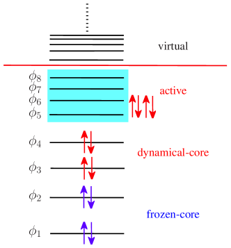
Figure 1: Pictorial explanation of the TD-CASSCF concept, illustrating a 12-electron system with two frozen-core (orbitals 1 and 2), two dynamical-core (3 and 4), and four active orbitals (5 to 8). Solving the orbital-EOM guarantees the variational splitting, in a time-dependent sense, of core-active, core-virtual, and active-virtual orbital subspaces.

The equation of motion (EOM) of our method, called TD-CASSCF, is derived based on the time-dependent variational principle (TDVP) Frenkel (1934); L$\ddot{\textrm{o}}$wdin and Mukherjee (1972); Moccia (1973), as detailed in Sec. II. It guarantees the best possible solution using the total wavefunction expressed as Eq. (4). The fully correlated active space allows to describe ionization processes which involve the strong correlation due to the breaking closed-shell symmetry (discussed in Sec. III.2). It can also include multichannel and multielectron effects (discussed in Sec. III.3). The dynamical core orbitals account for the effect of field-induced core polarizations. In whole, the TD-CASSCF method enables compact yet accurate representation of multielectron dynamics, if the active space is chosen correctly according to the physical processes of interest.

This paper proceeds as follows. In Sec. II, the details of the TD-CASSCF method are described. Then in Sec. III, the TD-CASSCF method is numerically assessed for ionization dynamics of one-dimensional multielectron models. Finally, Sec. IV concludes this work and discusses future prospects. Appendix A provides the definition and computational details for real-space domain-based ionization probabilities. The Hartree atomic units are used throughout unless otherwise noted.

II Theory

In this section, we derive the EOMs for the TD-CASSCF method. To this end, first we give the rigorous definitions of the MCTDHF, MCSCF, CASSCF, and general multiconfiguration ansatz for the total wavefunction in Sec. II.1. Next in Sec. II.2, the EOMs of orbitals and CI coefficients for the general multiconfiguration wavefunctions are discussed by reviewing the work of Miranda et al Miranda et al. (2011). Then we specialize the general formulation to the TD-CASSCF method in Sec. II.3 to derive the explicit EOMs, and discuss its computational aspects in Sec. II.4.

II.1 Multiconfiguration wavefunctions

Our formulation is determinant-based Olsen et al. (1988); Hochstuhl and Bonitz (2011) within the spin-restricted treatment, i.e., using the same spatial orbitals for up- and down-spin electrons. We define $n$ occupied spatial orbitals $\{\phi_{p};p=1,2,\cdot\cdot\cdot,n\}$ and $N_{b}-n$ virtual orbitals $\{\phi_{a};a=n+1,n+2,\cdot\cdot\cdot,N_{b}\}$, here $N_{b}$ is the dimension of the spinless one-particle Hilbert space, determined by e.g., the number of grid points to discretize the orbitals or the number of intrinsic single-particle basis functions to expand the orbitals. The indices $\{p,q,r,s\}$, $\{a,b\}$, and $\{\mu,\nu,\lambda,\gamma,\delta\}$ are used to label occupied, virtual, and general (occupied + virtual) orbitals, respectively, and $\{\sigma,\tau\}\in\{\alpha,\beta\}$ label spin eigenfunctions. In the followings, Einsteins’s summation convention is applied for repeated upper and lower orbital indices within a term, with summation ranges implicit as above. The orbitals are assumed to be orthonormal all the time,

$$\langle\phi_{\mu}(t)|\phi_{\nu}(t)\rangle\equiv\int\!d\bm{r}\phi^{*}_{\mu}(t)\phi_{\nu}(t)=\delta^{\mu}_{\nu},$$ (5)

where $\delta^{\mu}_{\nu}$ denotes the Kronecker delta. The Slater determinants $\Phi_{\rm I}(t)$ in Eq. (2) are constructed, as usual, from the occupied orbitals $\{\phi_{p}\}$, and given in the occupation number representation Helgaker et al. (2002); Hochstuhl and Bonitz (2011) as

$$|I(t)\rangle = |I^{\alpha}_{1}I^{\alpha}_{2}\cdot\cdot\cdot I^{\alpha}_{n}I^{\beta}_{1}I^{\beta}_{2}\cdot\cdot\cdot I^{\beta}_{n};t\rangle$$ (6)

$$= \prod_{p=1}^{n}(\hat{a}^{\dagger}_{p\alpha})^{I^{\alpha}_{p}}(\hat{a}^{\dagger}_{p\beta})^{I^{\beta}_{p}}|vac\rangle,$$

where $\hat{a}^{\dagger}_{\mu\sigma}$ (and $\hat{a}_{\mu\sigma}$ appearing below) is the Fermion creation (destruction) operator for 2$N_{b}$ spin-orbitals $\{\phi_{\mu}\}\otimes\{\alpha,\beta\}$. The integer array $\{I^{\sigma}_{p}=0,1\}$ specifies the occupancy of each spin-orbital, where $\sum_{p=1}^{n}I^{\sigma}_{p}=N^{\sigma}$, with $N^{\sigma}$ being the number of $\sigma$-spin electrons, and $N=N^{\alpha}+N^{\beta}$. The time-dependence of the occupation number vector $|I(t)\rangle$ is implicit in the spatial orbitals.

We focus on the dynamics induced by spin-independent external fields, and the initial wavefunction is assumed to be the spin eigenfunction. Therefore the total and projected spin operators, $\hat{S}^{2},\hat{S}_{z}$ are the constants of motion. Each Slater determinant is the eigenfunction of $\hat{S}_{z}$ with eigenvalue $N^{\alpha}-N^{\beta}$, while not generally of $\hat{S}^{2}$. The total wavefunction is spin-adapted, however, since the initial state is prepared by the variational optimization of CI coefficients, which automatically gives proper spin combinations.

Throughout this paper, the term MCTDHF is used for the method based on the full-CI expansion using $n$ occupied orbitals:

$$|\Psi_{\rm MCTDHF}(t)\rangle=\sum_{I}^{\Pi_{\rm FCI}}C_{I}(t)|I(t)\rangle,$$ (7)

with $I$ varying freely in the full-CI space $\Pi_{\rm FCI}$, spanned by all the determinants generated from the 2$n$ occupied spin-orbitals. This is the current standard of the MCTDHF method as mentioned in Sec. I. Note that Miranda et al Miranda et al. (2011) used the term MCTDHF in a broader sense to denote approaches based on the general multiconfiguration wavefunctions. To be definite, we call the general ansatz as MCSCF:

$$|\Psi_{\rm MCSCF}(t)\rangle=\sum_{I}^{\Pi}C_{I}(t)|I(t)\rangle,$$ (8)

with the general CI space $\Pi$ defined as any arbitrary subspace of $\Pi_{\rm FCI}$, $\Pi=\{|I\rangle\in\Pi_{\rm FCI};C_{I}(t)\equiv/\hskip 5.0pt0\}$. A trivial example of this class is the single-determinant HF wavefunction for closed-shell singlet or open-shell high-spin states. The only nontrivial applications of Eq. (8) to the time-dependent problems made thus far is the general open-shell TDHF approaches formulated in Ref. Miranda et al. (2011), in which the CI coefficients are determined by the spin-symmetry and time-independent.

The most successful MCSCF method in quantum chemistry is the CASSCF (also known as fully optimized reaction space) method introduced in Sec. I [Eq. (4)], in which the CI expansion is limited to the space spanned by Slater determinants that include $n_{\rm C}$ doubly occupied core orbitals, called the CASCI space $\Pi_{\rm CAS}$:

$$|\Psi_{\rm CASSCF}(t)\rangle=\sum_{I}^{\Pi_{\rm CAS}}C_{I}(t)|I(t)\rangle,$$ (9)

$$|I\rangle=\prod_{i=1}^{n_{\rm C}}\hat{a}^{\dagger}_{i\alpha}\hat{a}^{\dagger}_{i\beta}\prod_{t=n_{\rm C}+1}^{n}(\hat{a}^{\dagger}_{t\alpha})^{I^{\alpha}_{t}}(\hat{a}^{\dagger}_{t\beta})^{I^{\beta}_{t}}|vac\rangle,$$ (10)

with $\sum_{t}I^{\sigma}_{t}=N^{\sigma}_{\rm A}$ being the number of $\sigma$-spin active electrons satisfying $N^{\sigma}_{\rm A}=N^{\sigma}-N_{\rm C}/2$ and $N_{\rm A}=N^{\alpha}_{\rm A}+N^{\beta}_{\rm A}$. Hereafter, we use orbital indices $\{i,j,k,l\}$ for core- and $\{t,u,v,w,x\}$ for active-orbitals, while keeping $\{p,q,r,s\}$ for general occupied (core + active) orbitals. Following the convention in the electronic structure theory Szabo and Ostlund (1996); Helgaker et al. (2002), we use the acronym CASSCF($N_{\rm A},n_{\rm A}$) to denote the CASSCF wavefunction with $N_{\rm A}$ active electrons and $n_{\rm A}$ active orbitals. The MCTDHF wavefunction with $n$ occupied orbitals is identical to CASSCF($N,n$) and denoted as MCTDHF($n$). See Fig. 1, Eqs. (3) and (4) in Sec. I, and Eqs. (53) and (54) in Sec. III for intuitive understanding of these notations.

II.2 Equations of motion for MCSCF wavefunctions

Recently, Miranda et al discussed EOMs for MCSCF wavefunctions Miranda et al. (2011). Although their main motivation was the fixed-CI formulations, they also presented important equations applicable to the general MCSCF wavefunctions (See Sec. IV of Ref. Miranda et al. (2011)). Here we follow the essentials of their development to obtain Eqs. (20) and (21) below.

The spin-free second-quantized Hamiltonian is given by

$$\hat{H}=h^{\mu}_{\nu}\hat{E}^{\mu}_{\nu}+\frac{1}{2}g^{\mu\lambda}_{\nu\gamma}\hat{E}^{\mu\lambda}_{\nu\gamma},$$ (11)

where $h^{\mu}_{\nu}$ and $g^{\mu\lambda}_{\nu\gamma}$ are the one- and two-electron Hamiltonian matrix elements,

$$h^{\mu}_{\nu}=\int d\bm{r}\phi^{*}_{\mu}(\bm{r})h\left(\bm{r},\bm{\nabla}_{r}\right)\phi_{\nu}(\bm{r}),$$ (12)

$$g^{\mu\lambda}_{\nu\gamma}=\int\!\!\!\int\!d\bm{r}_{1}d\bm{r}_{2} \phi^{*}_{\mu}(\bm{r}_{1})\phi^{*}_{\lambda}(\bm{r}_{2})V_{ee}(\bm{r}_{1},\bm{r}_{2})$$

$$\times \phi_{\nu}(\bm{r}_{1})\phi_{\gamma}(\bm{r}_{2}),$$ (13)

with $h$ consisting of kinetic, nucleus-electron, and external laser terms, and $V_{ee}$ being the electron-electron interaction, and

$$\hat{E}^{\mu}_{\nu}=\sum_{\sigma}\hat{a}^{\dagger}_{\mu\sigma}\hat{a}_{\nu\sigma},$$ (14)

$$\hat{E}^{\mu\lambda}_{\nu\gamma}=\sum_{\sigma\tau}\hat{a}^{\dagger}_{\mu\sigma}\hat{a}^{\dagger}_{\lambda\tau}\hat{a}_{\gamma\tau}\hat{a}_{\nu\sigma}=\hat{E}^{\mu}_{\nu}\hat{E}^{\lambda}_{\gamma}-\hat{E}^{\mu}_{\gamma}\delta^{\lambda}_{\nu}.$$ (15)

Following the TDVP Frenkel (1934); L$\ddot{\textrm{o}}$wdin and Mukherjee (1972); Moccia (1973), the action integral $S$,

$$S[\Psi]=\int_{t_{0}}^{t_{1}}\!dt\langle\Psi|\left(\hat{H}-{\rm i}\frac{\partial}{\partial t}\right)|\Psi\rangle,$$ (16)

is made stationary,

$$\delta S=\int_{t_{0}}^{t_{1}}\!dt \left\{\langle\delta\Psi|\left(\hat{H}|\Psi\rangle-{\rm i}|\dot{\Psi}\rangle\right)\right.$$

$$+ \left.\left(\langle\Psi|\hat{H}+{\rm i}\langle\dot{\Psi}|\right)|\delta\Psi\rangle\right\}=0,$$ (17)

with respect to allowed variations $\delta\Psi$ of the total wavefunction, where $\dot{\Psi}\equiv\partial\Psi/\partial t$. The time derivative of $\delta\Psi$ is integrated out by part, assuming $\delta\Psi(t_{0})=\delta\Psi(t_{1})=0$. See Ref. Moccia (1973) for the formal discussion on the validity of this procedure. By taking the orbital orthonormality into account, the variations and the time derivatives of an orbital $\phi_{\mu}$ can be written as $\delta\phi_{\mu}=\phi_{\nu}\Delta^{\nu}_{\mu}$, and ${\rm i}\dot{\phi}_{\mu}=\phi_{\nu}R^{\nu}_{\mu}$, respectively, with $R^{\mu}_{\nu}\equiv{\rm i}\langle\phi_{\mu}|\dot{\phi}_{\nu}\rangle$. The matrix $\Delta$ is anti-Hermitian, while $R$ is Hermitian Miranda et al. (2011). Then, the allowed variation and the time derivative of the total wavefunction are compactly given by

$$|\delta\Psi\rangle=\sum_{I}^{\rm\Pi}|I\rangle\delta C_{I}+\hat{\Delta}|\Psi\rangle,$$ (18)

$${\rm i}|\dot{\Psi}\rangle={\rm i}\sum_{I}^{\rm\Pi}|I\rangle\dot{C}_{I}+\hat{R}|\Psi\rangle,$$ (19)

where $\delta C_{I}$ and $\dot{C}_{I}$ are the variation and the time derivative of CI coefficient $C_{I}$, and $\hat{\Delta}=\Delta^{\mu}_{\nu}\hat{E}^{\mu}_{\nu}$, $\hat{R}=R^{\mu}_{\nu}\hat{E}^{\mu}_{\nu}$. Inserting Eqs. (19) and (19) and their Hermitian conjugates $\langle\delta\Phi|$ and $-{\rm i}\langle\dot{\Phi}|$ into Eq. (II.2), and requiring the equality for individual variations $\delta C_{I}(t)$ and $\Delta^{p}_{q}(t)$, after some algebraic manipulations Miranda et al. (2011) we have

$${\rm i}\dot{C}_{I}=\langle I|\bar{H}|\Psi\rangle,$$ (20)

$$\langle\Psi|\bar{H}(1-\hat{\Pi})\hat{E}^{\mu}_{\nu}|\Psi\rangle-\langle\Psi|\hat{E}^{\mu}_{\nu}(1-\hat{\Pi})\bar{H}|\Psi\rangle=0,$$ (21)

where $\bar{H}=\hat{H}-\hat{R}$, and $\hat{\Pi}=\sum_{I\in\Pi}|I\rangle\langle I|$ is the configuration projector onto the general CI space $\Pi$. The system of equations, Eqs. (20) and (21), is to be solved for ${\rm i}\dot{C}_{I}$ and $R$, which determine the time-dependence of CI coefficients and orbitals, respectively. In Ref. Miranda et al. (2011), these equations appeared as an intermediate to derive the MCTDHF equation, rather than as the final result. Here we emphasize that Eqs. (20) and (21) are valid for general MCSCF wavefunction fit into the form of Eq. (8). Equation (21) is also extensively discussed by Miyagi and Madsen in their recent development of MCTDHF method with restricted CI expansions Miyagi and Madsen .

II.3 TD-CASSCF equations of motion

II.3.1 Orbital equations of motion

Now we apply the CASSCF constraint defined in Sec. II.1 to the general orbital-EOM derived in Sec. II.2. Equation (21), with $\hat{\Pi}$ replaced by $\hat{\Pi}_{\rm CAS}$, reduces to a trivial identity for an orbital pair $\{\mu,\nu\}$ belonging to a same orbital subspace (core, active, or virtual), since the singly replaced determinants, $\hat{E}^{i}_{j}|I\rangle=2\delta^{i}_{j}|I\rangle$, $\hat{E}^{t}_{u}|I\rangle$, or $\hat{E}^{a}_{b}|I\rangle=0$, either fall within $\Pi_{\rm CAS}$ or vanish, and the configuration projector $1-\hat{\Pi}_{\rm CAS}$ eliminates such contributions. We refer to these intra-subspace orbital rotations $\{\hat{E}^{i}_{j},\hat{E}^{t}_{u},\hat{E}^{a}_{b}\}$ as redundant, since the total wavefunction is invariant under such orbital transformations, if accompanied by the corresponding transformation of CI coefficients Helgaker et al. (2002); Caillat et al. (2005).

The redundant orbital rotations can be excluded in varying our action functional in Eq. (18), since their effects to $\delta\Psi$ are taken into account by the CI variations $\delta C_{I}$. On the other hand, for $\{\mu,\nu\}$ belonging to different orbital subspaces (core-active, core-virtual, or active-virtual), the projector $\hat{\Pi}_{\rm CAS}$ can be dropped in Eq. (21), and we have a simpler expression,

$$\langle\Psi|\left[\hat{H}-\hat{R},\hat{E}^{\mu}_{\nu}\right]|\Psi\rangle=0,$$ (22)

with $\hat{E}^{\mu}_{\nu}=\{\hat{E}^{a}_{p},\hat{E}^{p}_{a},\hat{E}^{t}_{i},\hat{E}^{i}_{t}\}$, constituting the non-redundant orbital rotations. The general orbital-EOM of Eq. (21) is thus reduced to Eq. (22), which is to be solved only for the non-redundant orbital pairs.

It is fascinating to see an analogy in Equation (22) with the time-independent MCSCF theory; It is formally identical to the generalized Brillouin condition of the stationary wavefunction Levy and Berthier (1968, 1969), if we replace $\hat{H}-\hat{R}$ with $\hat{H}$. Thus, the remaining derivations are parallel to the time-independent theory. We can explicitly write down the matrix elements of Eq. (22) to obtain

$$R^{\mu}_{\lambda}D^{\lambda}_{\nu}-D^{\mu}_{\lambda}R^{\lambda}_{\nu}=F^{\mu}_{\nu}-F^{\nu*}_{\mu},$$ (23)

$$F^{\mu}_{\nu}=h^{\mu}_{\lambda}D^{\lambda}_{\nu}+g^{\mu\gamma}_{\lambda\delta}P^{\lambda\delta}_{\nu\gamma},$$ (24)

where $D^{\mu}_{\nu}\equiv\langle\Psi|\hat{E}^{\nu}_{\mu}|\Psi\rangle$ and $P^{\mu\lambda}_{\nu\gamma}\equiv\langle\Psi|\hat{E}^{\nu\gamma}_{\mu\lambda}|\Psi\rangle$ are one- and two-electron reduced density matrix (RDM) elements, respectively. The matrix $F$ is called the generalized Fock matrix, whose Hermiticity, leading to vanishing right-hand side of Eq. (23), is the stationary condition with respect to the orbital variations. Roos et al. (1980); Roos (1987); Schmidt and Gordon (1998); Helgaker et al. (2002)

The nonzero density matrix elements of the CASSCF wavefunction are $D^{i}_{j}=2\delta^{i}_{j},D^{t}_{u},P^{ij}_{kl}=4\delta^{i}_{k}\delta^{j}_{l}-2\delta^{i}_{l}\delta^{j}_{k},P^{ti}_{ui}=2D^{t}_{u},P^{ti}_{iu}=-D^{t}_{u}$ and $P^{tu}_{vw}$. Then the required generalized Fock matrix elements read Roos et al. (1980)

$$F^{\mu}_{i}=2(f^{\mu}_{i}+G^{\mu}_{i}),$$ (25)

$$F^{\mu}_{t}=f^{\mu}_{u}D^{u}_{t}+\left({\mit\Gamma}_{t}\right)^{\mu}_{t},$$ (26)

where the matrices $f$, $G$, and ${\mit\Gamma}_{t}$ represent, respectively, operators $\hat{f}$, $\hat{G}$, and $\hat{\mit\Gamma}_{t}$ given by

$$\hat{f}=\hat{h}^{\rm FC}+\sum_{j}^{\rm d.c.}\left(2\hat{J}_{j}-\hat{K}_{j}\right),$$ (27)

$$\hat{G}=\left(\hat{J}^{t}_{u}-\frac{1}{2}\hat{K}^{t}_{u}\right)D^{u}_{t},$$ (28)

$$\hat{\mit\Gamma}_{t}|\phi_{t}\rangle=\hat{W}^{u}_{w}|\phi_{v}\rangle P^{vw}_{tu},$$ (29)

$$\hat{h}^{\rm FC}(t)=\hat{h}(t)+\sum_{j}^{\rm f.c.}\left(2\hat{J}_{j}(0)-\hat{K}_{j}(0)\right),$$ (30)

where summation $j$ in Eqs. (27) and (30) are restricted within dynamical-core (${\rm d.c.}$) and frozen-core (${\rm f.c.}$) subspaces, respectively. The operators $\hat{f}$ and $\hat{G}$ are universal and Hermitian, while $\hat{\mit\Gamma}_{t}$ is defined with an active orbital $\phi_{t}$ to be applied from the left, and non-Hermitian. We define Coulomb $\hat{J}$, exchange $\hat{K}$, and general $\hat{W}$ mean field operators as $\hat{J}_{p}=\hat{J}^{p}_{p},\hat{K}_{p}=\hat{K}^{p}_{p},\hat{J}^{p}_{q}=\hat{W}^{p}_{q},\hat{K}^{p}_{q}|\phi_{r}\rangle=\hat{W}^{p}_{r}|\phi_{q}\rangle$, where $\hat{W}^{p}_{q}$ is local Kato and Kono (2008) and given in the coordinate space as

$$W^{p}_{q}(\bm{r})=\int\!d\bar{\bm{r}}\phi^{*}_{p}(\bar{\bm{r}})V_{ee}(\bm{r},\bar{\bm{r}})\phi_{q}(\bar{\bm{r}}).$$ (31)

In Eq. (30), time argument $t$ is explicitly attached to emphasize that the time-dependence of the frozen-core dressed one-electron Hamiltonian $\hat{h}^{\rm FC}(t)$ comes entirely from the external laser field contribution in $\hat{h}(t)$. Now Eq. (23) for the time derivative matrix $R^{\mu}_{\nu}={\rm i}\langle\phi_{\mu}|\dot{\phi}_{\nu}\rangle$ can be worked out for inter-subspace (non-redundant) elements:

$$\begin{array}[]{ll}R^{\mu}_{i}=R^{i*}_{\mu}=0&(i\in{\rm f.c.}),\end{array}$$ (33)

$$\begin{array}[]{ll}R^{a}_{i}=R^{i*}_{a}=f^{a}_{i}+G^{a}_{i}&(i\in{\rm d.c.}),\end{array}$$ (35)

$$R^{a}_{t}=R^{t*}_{a}=f^{a}_{t}+\left({\mit\Gamma}_{u}\right)^{a}_{u}\left(D^{-1}\right)^{u}_{t},$$ (36)

$$\begin{array}[]{c}R^{t}_{i}=R^{i*}_{t}=f^{t}_{i}+\left(\bar{D}^{-1}\right)^{t}_{u}\left\{G^{u}_{i}-\left({\mit\Gamma}_{u}\right)^{u}_{i}\right\}\\ (i\in{\rm d.c.}),\end{array}$$ (39)

with $\bar{D}^{t}_{u}=2\delta^{t}_{u}-D^{t}_{u}$, and for intra-subspace (redundant) elements:

$$R^{\mu}_{\nu}=\langle\phi_{\mu}|\hat{\theta}(t)|\phi_{\nu}\rangle,$$ (40)

where $\hat{\theta}(t)$ can be an arbitrary one-electron Hermitian operator Caillat et al. (2005); Kato and Kono (2004); Miranda et al. (2011), reflecting the invariance of the total wavefunction against the redundant orbital transformations.

One could, in principle, directly work with Eqs. (33)–(40) in the matrix formulation Kato and Kono (2004), which determines the time dependence of occupied $\left\{\phi_{p}(t)\right\}$, as well as virtual $\left\{\phi_{a}(t)\right\}$ orbitals. However, it is beneficial to introduce the orbital projector $\hat{Q}=\sum_{a}|\phi_{a}\rangle\langle\phi_{a}|=1-\sum_{p}|\phi_{p}\rangle\langle\phi_{p}|$ onto the virtual orbital space, to avoid (using the assumed completeness) explicitly dealing with numerous virtual orbitals Caillat et al. (2005); Beck et al. (2000). Thus we arrive at the final expression of EOMs for dynamical-core and active orbitals as follows:

$${\rm i}|\dot{\phi}_{i}\rangle=\hat{Q}\left(\hat{f}+\hat{G}\right)|\phi_{i}\rangle+|\phi_{p}\rangle R^{p}_{i},$$ (41)

$${\rm i}|\dot{\phi}_{t}\rangle=\hat{Q}\left\{\hat{f}|\phi_{t}\rangle+\hat{\mit\Gamma}_{u}|\phi_{u}\rangle\left(D^{-1}\right)^{u}_{t}\right\}+|\phi_{p}\rangle R^{p}_{t},$$ (42)

and $R$ is determined by Eqs. (39) and (40) with a particular choice of $\hat{\theta}(t)$. Solving these equations guarantees the optimal separation, in the TDVP sense, of frozen-core, dynamical-core, active, and virtual orbital subspaces, as illustrated in Fig. 1. This ensures the gauge-invariance of the TD-CASSCF method, since the orbital subspaces are stable against single excitations [Eq. (22)] arising with the transformation, e.g., from the length gauge to the velocity gauge.

II.3.2 CI equations of motion

The general CI-EOM of Eq. (20) is specialized to the TD-CASSCF method as

$${\rm i}\dot{C}_{I}=\sum_{J}^{\Pi_{\rm CAS}}\left(H^{\rm A}_{IJ}-\delta_{IJ}E^{\rm A}-R_{IJ}\right)C_{J},$$ (43)

where $R_{IJ}=\langle I|\hat{R}|J\rangle$, $E^{\rm A}$ and $H^{\rm A}_{IJ}$ are active orbital contributions to the total energy and determinant basis Hamiltonian matrix elements, respectively,

$$E\equiv\langle\Psi|\hat{H}|\Psi\rangle=E^{\rm C}+E^{\rm A},$$ (44)

$$\langle I|\hat{H}|J\rangle=\delta_{IJ}E^{\rm C}+H^{\rm A}_{IJ},$$ (45)

where

$$E^{\rm C}=\sum_{i}^{\rm d.c.}\left\{\left(h^{\rm FC}\right)^{i}_{i}+f^{i}_{i}\right\},$$ (46)

$$E^{\rm A}=f^{t}_{u}D^{u}_{t}+\frac{1}{2}g^{tv}_{uw}P^{uw}_{tv},$$ (47)

$$H^{\rm A}_{IJ}=f^{t}_{u}(D_{IJ})^{u}_{t}+\frac{1}{2}g^{tv}_{uw}(P_{IJ})^{uw}_{tv},$$ (48)

where $(D_{IJ})^{u}_{t}=\langle I|\hat{E}^{t}_{u}|J\rangle$, and $(P_{IJ})^{uw}_{tv}=\langle I|\hat{E}^{tv}_{uw}|J\rangle$. In Eq. (43), we make a particular phase choice, ${\rm i}\langle\Psi|\dot{\Psi}\rangle=0$, by extracting the dynamical phase $\exp\!\left[-{\rm i}\int^{t}dt^{\prime}E(t^{\prime})\right]$ from the total wavefunction. This stabilizes the CI-EOM especially when we have a large active space.

II.4 Computational remarks

The TD-CASSCF method includes as special cases both TDHF and MCTDHF methods, thus bridges the gap between the uncorrelated and fully correlated descriptions in a flexible way. A practical advantage of this generality is that a computational code written for the TD-CASSCF method can be used also for single-determinant TDHF and MCTDHF calculations, by setting {$n_{\rm C}=n$, $n_{\rm A}=0$} and $\{n_{\rm C}=0$, $n_{\rm A}=n$}, respectively. It can also execute open-shell TDHF calculation with fixed CI coefficients Miranda et al. (2011). One indeed finds close similarity between TD-CASSCF EOMs Eqs. (41–43) and those of the MCTDHF method (See e.g. Ref. Hochstuhl and Bonitz (2011)). Naively, ingredients of the TD-CASSCF EOMs are the compilation of those for TDHF (core orbitals) and MCTDHF (active orbitals and CI coefficients) methods. This means that an existing code for the MCTDHF method can be easily generalized to the TD-CASSCF method.

The computationally most demanding procedures required to integrate the TD-CASSCF EOMs are grouped into two categories:

1. Calculations of 2RDM elements $P^{tu}_{vw}$, and the two-electron contributions of Eq. (43),

   $${\rm i}\dot{C}_{I}\longleftarrow\frac{1}{2}\sum_{J}^{\Pi_{\rm CAS}}g^{tv}_{uw}(P_{IJ})^{uw}_{tv}C_{J}.$$ (49)

   The amount of work in these procedures roughly scales as $O(N^{2}_{\rm A}(n_{\rm A}-N_{\rm A})^{2}N_{\rm det})$ if $N^{\alpha}_{\rm A}=N^{\beta}_{\rm A}$, (see Ref. Olsen et al. (1988) for more details), where $N_{\rm det}$ is the number of determinants in $\Pi_{\rm CAS}$ which in turn scales factorially with the number of active electrons $N_{\rm A}$.

2. Calculations of the mean fields $W^{p}_{q}(\bm{r})$, two-electron integrals $g^{tv}_{uw}$, and the 2RDM contributions in Eq. (42),

   $${\rm i}\dot{\phi}_{t}\longleftarrow\hat{W}^{v}_{w}|\phi_{x}\rangle P^{xw}_{uv}\left(D^{-1}\right)^{u}_{t}.$$ (50)

   The computational cost of these steps depend explicitly on the number of grid points (or basis functions) $N_{b}$, as $O(n^{2}N^{2}_{b})$ for the mean fields and $O(n^{4}_{\rm A}N_{b})$ for the others.

Important cost reductions are achieved for both procedures (A) and (B) by the TD-CASSCF method adopting core orbitals, compared to the MCTDHF method with the same number of occupied orbitals. The speed-up and resource savings for procedure (A) is substantial due to the decreased CI dimension. This is especially the case if $N_{\rm A}\ll N$, which is expected for an electronic structure with a few weakly-bound valence and large numbers of physically inactive core electrons. The cost reduction for procedure (B) is not as drastic as for (A), since the amount of arithmetics $O(n^{2}N^{2}_{b})$ of computing mean fields $W^{p}_{q}(\bm{r})$ is independent of the CAS structure (only related to $n$). The computations of two electron integrals and Eq. (50) become much faster through restricting the orbital indices within the active instead of all occupied orbitals. Relative importance of these bottlenecks largely depends on the problem at hand, and on the spatial representation of the orbitals and electron-electron interactions. This point will be discussed in Sec. III.3.

III Numerical results and discussions

In this section, we apply the TD-CASSCF method to the ionization dynamics of one-dimensional (1D) multielectron model molecules. The effective 1D Hamiltonian for $N$ electrons in the potential of $M$ fixed nuclei interacting with an external laser electric field $E(t)$ is taken as

$$H=\sum_{i}^{N}\left\{-\frac{1}{2}\frac{\partial^{2}}{\partial x^{2}_{i}}-\sum_{a}^{M}\frac{Z_{a}}{\sqrt{(x_{i}-X_{a})^{2}+c}}-E(t)x_{i}\right\}+\sum_{i>j}^{N}\frac{1}{\sqrt{(x_{i}-x_{j})^{2}+d}},$$ (51)

where $x_{i}\,(i=1,\cdots,N)$ is the position of the $i$-th electron, $\bm{X}=\{X_{a}\}$ and $\bm{Z}=\{Z_{a}\}$ $(a=1,\cdots,M)$ are the positions and charges of nuclei, and $c$ and $d$ adjust the soft Coulomb operators of electron-nuclear and electron-electron interactions, respectively. The electron-laser interaction is included within the dipole approximation and in the length gauge. Note that the TD-CASSCF method is gauge-invariant as mentioned in Sec. II.3.1. We have performed some of the calculations described below also in the velocity gauge, and confirmed that the results are virtually identical to those in the length gauge.

In this work, we make the simplest choice of $\hat{\theta}(t)\equiv 0$ in Eqs. (40), and therefore $R_{IJ}=0$ in Eq. (43). The orbital-EOMs are discretized on an equidistant grid of spacing $\Delta x=0.4$ (finer grid with $\Delta x=0.1$) is used for drawing Figs. 2-4), within a simulation box $|x|<L$ with $L=600$. An absorbing boundary is implemented by the mask function of $\cos^{1/4}$ shape at 15% side edges of the box. The ground-state electronic structure is obtained by the imaginary time propagation with the fourth-order Runge-Kutta (RK4) algorithm with Schmidt orthonormalization of orbitals after each propagation Kato and Kono (2004). The real-time propagations use variable step-size embedded fourth- and fifth-order Runge-Kutta (VRK5) method. The kinetic energy operator $-\frac{1}{2}\frac{\partial^{2}}{\partial x^{2}_{i}}$ is evaluated by the eighth-order finite difference, and spatial integrations are replaced by grid summations using the trapezoidal rule. Further details of the computations are given separately below.

III.1 1D-LiH and LiH dimer models: Ground-state

We consider 1D lithium hydride (LiH) and LiH dimer models. The reason for choosing these models is that they represent the simplest examples of such electronic structures with (i) deeply bound orbitals, and (ii) several weakly bound orbitals, as shown below. These characteristics should be the key in the three-dimensional (3D) multielectron dynamics, where the existence of energetically closely-lying valence electrons is quite common, which requires to take both multichannel and multielectron effects into account. As discussed previously Jordan et al. (2006), cares have to be made for the physical soundness of 1D models. Nevertheless, we expect that the features (i) and (ii) are transferable, and 1D applications can elucidate advantages and limitations of theoretical methods, before applied to real 3D systems.

For LiH, we set molecular parameters as $\bm{Z}=\{3,1\}$ and $\bm{X}=\{-1.15,1.15\}$. For (LiH)₂, $\bm{Z}=\{3,1,3,1\}$ and $\bm{X}=\{-4.05,-1.75,+1.75,+4.05\}$. The soft Coulomb parameters $c=0.5$ and $d=1$ are used, since an often-made choice of $c=d=1$ Balzer et al. (2010a, b) was found to overemphasize the electron-electron repulsion. The above molecular parameters correspond to the equilibrium bond length $r=2.3$ of Li-H and intermolecular distance $R=3.5$ of LiH–LiH, as shown in Fig. 2, which plots several cuts of the adiabatic energy surface of (LiH)₂,

$$E(r,R)=\langle\Psi|H|\Psi\rangle+\sum_{a>b}^{M}\frac{Z_{a}Z_{b}}{|X_{a}-X_{b}|}.$$ (52)

The energy surface with parameters $c=d=1$ predicted no stable LiH dimer in this nuclear configuration, relative to the separated LiH molecules.

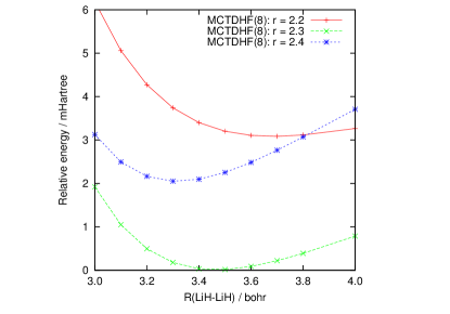
Figure 2: Several cuts of the adiabatic energy surface $E(r,R)$ of the 1D-(LiH)₂ model obtained by the MCTDHF($8$) method. The total energy of Eq. (52) is plotted against intermolecular LiH$\cdot\cdot\cdot$LiH distance $R$ for several bond lengths $r$ of LiH, constrained to be the same for two LiH molecules.

To make a sensible comparison among methods with different active spaces, we consider the following wavefunctions for LiH:

$$\Psi_{{\rm HF}} : \phi^{2}_{1}\phi^{2}_{2},$$ (53a)

$$\Psi_{{\rm CASSCF}(2,n)} : \phi^{2}_{1}\left(\phi_{2}\phi_{3}...\phi_{n+1}\right)^{2},$$ (53b)

$$\Psi_{{\rm MCTDHF}(n+1)} : \left(\phi_{1}\phi_{2}\phi_{3}...\phi_{n+1}\right)^{4},$$ (53c)

and for (LiH)₂:

$$\Psi_{{\rm HF}} : \phi^{2}_{1}\phi^{2}_{2}\phi^{2}_{3}\phi^{2}_{4},$$ (54a)

$$\Psi_{{\rm CASSCF}(2,n-1)} : \phi^{2}_{1}\phi^{2}_{2}\phi^{2}_{3}\left(\phi_{4}\phi_{5}...\phi_{n+2}\right)^{2},$$ (54b)

$$\Psi_{{\rm CASSCF}(4,n)} : \phi^{2}_{1}\phi^{2}_{2}\left(\phi_{3}\phi_{4}...\phi_{n+2}\right)^{4},$$ (54c)

$$\Psi_{{\rm MCTDHF}(n+2)} : \left(\phi_{1}\phi_{2}\phi_{3}...\phi_{n+2}\right)^{8},$$ (54d)

following the notations of Eqs. (3) and (4). The CASSCF and MCTDHF wavefunctions are designed to consist of the same number of occupied orbitals with increasing active orbitals.

Figures  3 and 4 show the shapes of the ground-state occupied HF orbitals and the one-electron probability density for LiH and (LiH)₂, respectively. As seen in Fig. 3(b) the nodeless first deepest HF orbital of LiH localizes at Li “atom”, while the second orbital is responsible for the formation of “chemical bond”, made from constructive superposition of the ground-state wavefunction of H and the second atomic orbital of Li, the node of the latter shifted to the bonding region. Figure 3(a) shows that the total electron density is well reproduced by HF method compared to the MCTDHF($8$) density. In Fig. 4(b), one sees that HF orbitals of (LiH)₂ can be clearly separated to the deeply-bound core (orbitals 1 and 2) and weakly-bound valence (orbitals 3 and 4) orbitals, the former keeping the atomic-orbital characters of Li, while the latter two orbitals delocalizing across the dimer. Again, as seen in Fig. 4(a), the total density is well reproduced by HF. Finally, it is observed that the tails of the total electron density are determined by the valence electrons both in LiH and (LiH)₂.

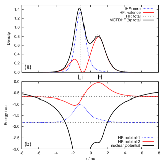
Figure 3: The ground-state electron density and occupied HF orbitals of the 1D-LiH model. (a) The total electron density by HF (black dashed) and MCTDHF($8$) (black thick solid) methods are compared. The two lines closely overlap each other. Also shown are the core (orbital 1) and valence (orbital 2) contributions to the total HF density. (b) The occupied HF orbitals are drawn in an arbitrary scale vertically shifted by orbital energies -1.82 (orbital 1) and -0.67 (orbitals 2). The solid curve and dashed vertical lines show the nuclear potential and positions of nuclei, respectively.

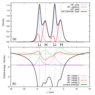
Figure 4: Same as Fig. 3 for the 1D-(LiH)₂ model. (a) The core and valence densities correspond to the contributions from orbitals 1 and 2, and orbitals 3 and 4, respectively. (b) The orbital energies are -1.85, -1.77, -0.73, and -0.60, for orbitals 1 to 4, respectively.

Table 1 summarizes the ground-state calculations. As seen in the table, there are significant gaps in total energies between methods with different numbers of active electrons. However the MCTDHF values for the other properties are reproduced rather well, by CASSCF($2,n$) and CASSCF($4,n$) methods for LiH and (LiH)₂, respectively. For instance, the difference in $E_{\rm tot}$ of CASSCF($4,8$) and MCTDHF($10$) for (LiH)₂ is approximately 12 mHartree, but those in IP and $\Delta_{2}$ are 0.05 eV (2 mHartree) and 0.003 eV (0.2 mHartree), respectively. This tells that the correlations responsible for these properties are those among the valence electrons.

The CASSCF($2,n$) active spaces of Eq. (54b) , with only two of four nearly degenerate electrons being correlated, are not physically sensible ones for (LiH)₂. Accordingly, the resulting dipole moment values are not much improved from the HF value. More seriously, the proper dissociation limit of such wavefunction to the equivalent LiH molecules cannot be defined well, i.e., the formation energy $\Delta_{2}$ cannot be obtained. This problem is due to the lack of the “size-extensivity”, Szabo and Ostlund (1996); Schmidt and Gordon (1998); Helgaker et al. (2002) which fails to guarantee the equal quality of the approximation for different electronic configurations. The size-inextensive treatment covers less and less electron correlation as systems grow larger.

Table 1: Total energy $E_{\rm tot}$ in atomic unit (a.u.), dipole moment $\langle x\rangle$ in a.u., first ionization potential IP in eV, LiH formation energy $\Delta_{1}$ in eV, and (LiH)₂ formation energy $\Delta_{2}$ in eV. Results of HF, CASSCF, and MCTDHF methods with varying active spaces are compared. The ionization potential (IP) is computed as the difference of the total energies of the neutral and cationic ground-states. The $\Delta_{1}$ is the difference of the energy of LiH and the sum of energies of Li and H, and $\Delta_{2}$ is the difference of the energy of (LiH)₂ and twice that of LiH. For computing $\Delta_{1}$ and $\Delta_{2}$ with CASSCF and MCTDHF methods, the active spaces for the fragments are the proper dissociation limit of the parent description of the complex. For HF calculations, the open-shell restricted HF method is used for doublet species. The $\Delta_{2}$ of CASSCF($2,n_{\rm A}$) methods are not available since their proper dissociation limits are not well defined.

		$E_{\rm tot}$	$\langle x\rangle$	IP	$\Delta_{1}$	$\Delta_{2}$
1D-LiH
$N_{\rm A}$ = 0
	HF	$-7.0664$	$-0.133$	$17.82$	$5.07$
$N_{\rm A}$ = 2
	CASSCF(2,2)	$-7.0819$	$-0.141$	$18.24$	$5.49$
	CASSCF(2,4)	$-7.0847$	$-0.141$	$18.32$	$5.57$
	CASSCF(2,8)	$-7.0847$	$-0.141$	$18.32$	$5.57$
$N_{\rm A}$ = 4
	MCTDHF(3)	$-7.0824$	$-0.141$	$18.15$	$5.51$
	MCTDHF(5)	$-7.0908$	$-0.142$	$18.32$	$5.46$
	MCTDHF(9)	$-7.0920$	$-0.142$	$18.35$	$5.48$
1D-(LiH)2
$N_{\rm A}$ = 0
	HF	$-14.1378$	$-0.231$	$15.57$		$0.135$
$N_{\rm A}$ = 2
	CASSCF(2,3)	$-14.1532$	$-0.236$	$15.99$		${\rm N/A}$
	CASSCF(2,5)	$-14.1534$	$-0.236$	$16.00$		${\rm N/A}$
	CASSCF(2,7)	$-14.1534$	$-0.236$	$16.00$		${\rm N/A}$
$N_{\rm A}$ = 4
	CASSCF(4,4)	$-14.1664$	$-0.245$	$15.80$		$0.071$
	CASSCF(4,6)	$-14.1726$	$-0.246$	$15.90$		$0.100$
	CASSCF(4,8)	$-14.1735$	$-0.246$	$15.92$		$0.114$
$N_{\rm A}$ = 8
	MCTDHF(6)	$-14.1682$	$-0.245$	$15.70$		$0.094$
	MCTDHF(8)	$-14.1822$	$-0.248$	$15.85$		$0.110$
	MCTDHF(10)	$-14.1859$	$-0.249$	$15.87$		$0.117$

III.2 1D LiH model: Ionization dynamics

Now we apply the TD-CASSCF method to the laser-driven electron dynamics of the 1D-LiH model. We use the three-cycle laser electric field of the following form;

$$E(t)=E_{0}\sin(\omega t)\sin^{2}\left(\pi\frac{t}{\tau}\right),\hskip 5.0pt0\leq t\leq\tau$$ (55)

with $\omega=0.06075$ (wavelength 750 nm), $\tau=6\pi/\omega$, and three different amplitudes $E_{0}$ = 0.0534, 0.107, and 0.151 corresponding to peak intensities $I_{0}$ = 1.0$\times$10¹⁴, 4.0$\times$10¹⁴, and 8.0$\times$10¹⁴ W/cm², respectively. The Keldysh parameters are 1.30, 0.65, and 0.46, respectively, for the three intensities. In view of the ground-state electronic structure of Fig. 3 and the above laser profile, one reasonably expects that the dominant physical process involved is the tunneling ionization from the highest occupied orbital in the static HF picture. Hence, we can speculate that the two-active-electron description TD-CASSCF($2,n_{\rm A}$) is necessary and sufficient for the accurate description of the dynamics, as will be confirmed below.

Figure 5 shows the time evolution of the dipole moment. First we observe the large difference in the results of TDHF and other methods. For the lowest intensity of 1.0$\times$10¹⁴ W/cm², the difference remains quantitative, largely due to the difference of the ground-state permanent dipole moment. For higher intensities, TDHF clearly underestimates the laser-driven large-amplitude electron motions. This is due to the fundamental inadequacy of the closed-shell description, Eq. (53a), of the tunneling ionization process, which involves spatially different motions of the ionizing and non-ionizing electrons. The TD-CASSCF($2,2$) brings substantial improvement over the TDHF, giving results with much better agreement with the MCTDHF ones. The convergent description in the TD-CASSCF($2,n_{\rm A}$) series is obtained at $n_{\rm A}=4$. The TD-CASSCF($2,n_{\rm A}$) with $n_{\rm A}\geq 4$ closely reproduce the results of MCTDHF method.

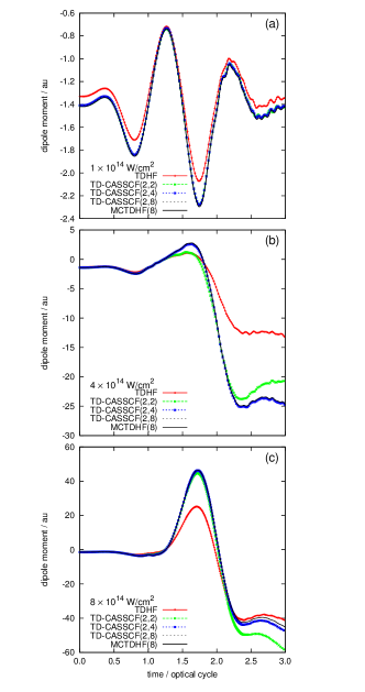
Figure 5: Dipole moment of the 1D-LiH model as a function of time, with peak intensities (a) 1$\times$10¹⁴, (b) 4$\times$10¹⁴, and (c) 8$\times$10¹⁴ W/cm².

Figure 6 plots the $n$-electron ionization probability $P_{n}$, defined for convenience as a probability to find $n$ electrons located outside a given distance $R_{\rm ion}=20$ (see Appendix A), of LiH as a function of time for the peak intensities (a) 4$\times$10¹⁴ and (b) 8$\times$10¹⁴ W/cm². No appreciable ionization is found with the lowest intensity. The probability of finding more than two ionized electrons is negligibly small for all intensities. As seen in Fig. 6, TD-CASSCF($2,4$) gives virtually the same results as MCTDHF($5$). The TDHF method, on the other hand, underestimates single ionization $P_{1}$ and, at the higher intensity, unphysically overestimates double ionization $P_{2}$. This is the consequence of forcing two valence electrons to travel with a single spatial orbital.

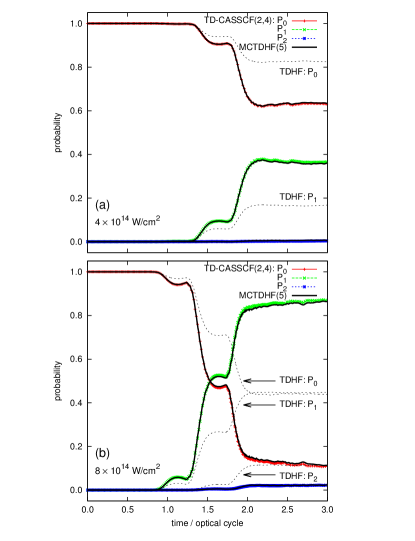
Figure 6: Ionization probabilities $P_{n}$ of the 1D-LiH model as a function of time, with peak intensities (a) 4$\times$10¹⁴ and (b) 8$\times$10¹⁴ W/cm². TDHF (black dotted), TD-CASSCF($2,4$) (colored), and MCTDHF($5$) (block solid) results are compared.

These results demonstrate that the TD-CASSCF($2,2$) constitutes the simplest method to describe the present dynamics in a physically correct way. Its total wavefunction can be written as

$$\Psi = \hat{A}\left[\phi_{1}\bar{\phi}_{1}\left\{C_{1}\phi_{2}\bar{\phi}_{2}+C_{2}\phi_{3}\bar{\phi}_{3}\right\}\right]$$ (56)

in the natural orbital representation Kutzelnigg (1963, 1964), where $\phi_{i}$ ($\bar{\phi_{i}}$) is an orbital occupied by up (down) spin electrons. The two-configuration CI part of Eq. (56) can be transformed back to the non-orthogonal expression [Eq. (1a)],

$$\Psi \propto \hat{A}\left[\phi_{1}\bar{\phi}_{1}\left\{(\psi_{2}\psi_{3}+\psi_{3}\psi_{2})\frac{1}{\sqrt{2}}(\alpha\beta-\beta\alpha)\right\}\right],$$ (57)

giving a clearer picture of different spatial motions of the two valence electrons, with Szabo and Ostlund (1996)

$$|\langle\psi_{1}|\psi_{2}\rangle|=\frac{|C_{1}|-|C_{2}|}{|C_{1}|+|C_{2}|}.$$ (58)

The flexibility inherent in Eqs. (56) or (57) enables a seamless transition from the closed-shell dominant ground-state ($|C_{1}|\gg|C_{2}|\Longleftrightarrow\langle\psi_{1}|\psi_{2}\rangle\approx 1$) to the single ionization limit ($|C_{1}|\approx|C_{2}|\Longleftrightarrow\langle\psi_{1}|\psi_{2}\rangle\approx 0$). The ionization dynamics, therefore, is characterized by the strong or static correlation Roos (1987); Szabo and Ostlund (1996); Schmidt and Gordon (1998); Helgaker et al. (2002) in the sense that it involves drastic changes of the configuration weights (the magnitudes of CI coefficients) with more than one determinants contributing significantly. The failure of single-determinant TDHF to describe the ionization process is attributed to the lack of this type of correlation.

For quantitatively accurate description of the dynamics, the above minimum CI wavefunction has to be improved by incorporating more-than-two active orbitals, as seen in the convergence of the dipole moments in Fig. 5 with respect to the number of active orbitals. The agreement of TD-CASSCF($2,n_{\rm A}$) and MCTDHF results indicates that the core electron correlation is not relevant, at the first approximation, for the ionization dynamics induced by the present laser field. The TD-CASSCF allows the compact representation of such physical situations.

III.3 1D-LiH dimer model: Ionization dynamics

In this section, we proceed to the multielectron dynamics of 1D-(LiH)₂ model. We assess TDHF, TD-CASSCF($2,7$), TD-CASSCF($4,8$), and MCTDHF($10$) methods. These active spaces are shown in Eq. (54) with $n=8$. The latter two are twice the size of those in TD-CASSCF($2,4$) and MCTDHF($5$) for LiH, respectively, which have been confirmed to provide the convergent description in Sec. III.2.

Figure 7 shows the temporal evolution of the dipole moment simulated with various methods. One clearly sees that TDHF and TD-CASSCF($2,7$) results show large deviations from MCTDHF($10$) ones, while TD-CASSCF($4,8$) reproduces the results of MCTDHF($10$) fairly well. This indicates that all the four valence electrons sketched in Fig. 4 actively participate in the field-induced ionization dynamics (this does not necessarily mean that the four electrons are ionized), while tightly bound core electrons remain non-ionized. For the ionizing electrons, the closed-shell description is inadequate as discussed in Sec. III.2.

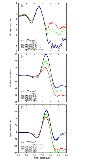
Figure 7: Dipole moment of the 1D-(LiH)₂ model as a function of time, with peak intensities (a) 1$\times$10¹⁴, (b) 4$\times$10¹⁴, and (c) 8$\times$10¹⁴ W/cm². Results of TDHF, TD-CASSCF($2,7$), TD-CASSCF($4,8$), MCTDHF($10$) methods are compared.

In Figs. 8 and 9, we compare the temporal evolution of the ionization probability $P_{n}$ with $R_{\rm ion}=20$ of (LiH)₂ computed by approximate methods and MCTDHF($10$). As can be seen from Fig. 8, both TDHF and TD-CASSCF($2,7$) methods tend to underestimate single ionization for all the examined intensities. The probability of finding more than two ionized electrons are found to be erroneous in an inconsistent way, thus not shown. In a striking contrast, TD-CASSCF($4,8$) well reproduces the ionization probability $P_{n}$ obtained with MCTDHF($10$) [Fig 9 (a)-(c)]. Slight deviation is seen only at the later stage of the pulse for the higher intensities. The inclusion of more active orbitals would further improve the agreement.

So far, all the core orbitals have been treated as dynamical core. In Fig. 9 (d)-(f), the ionization probability computed with TD-CASSCF($4,8$) with all the core orbitals treated as frozen, denoted TD-CASSCF($4,8$)-FC, are shown. It reproduces the results of MCTDHF($10$) almost as nicely as TD-CASSCF($4,8$) with dynamical-core orbitals, which indicates that the core polarization plays minor roles in the present dynamics.

It is worth noting that even at the lowest intensity 1.0$\times$10¹⁴ W/cm² dominated by single ionization, the TD-CASSCF($2,7$) fails to give an accurate value of $P_{1}$ but underestimates it roughly by half [Fig. 8 (d)]. This implies the importance of the multichannel ionization, which can be described correctly only when all the relevant orbitals are included in the active space. On the other hand, at higher intensities, the total wavefunction consists of the widespread superposition of the ground-, excited- and continuum-states. For a balanced description, each of these components has to be treated with an equal quality, which requires a size-extensive theory. The MCTDHF, as the exact theory within a given number of time-dependent bases, fulfills the size-extensivity condition. The TD-CASSCF with a proper active space preserves this important property of the MCTDHF. It is demonstrated by the accurate multiple ionization probabilities obtained by the TD-CASSCF($4,8$) method, up to $P_{4}$ for the highest intensity in Fig. 9 (c). The importance of selecting an appropriate active space is illustrated by the fact that the TD-CASSCF($4,n_{\rm A}$) is required for (LiH)₂, while the TD-CASSCF($2,n_{\rm A}$) is adequate for LiH.

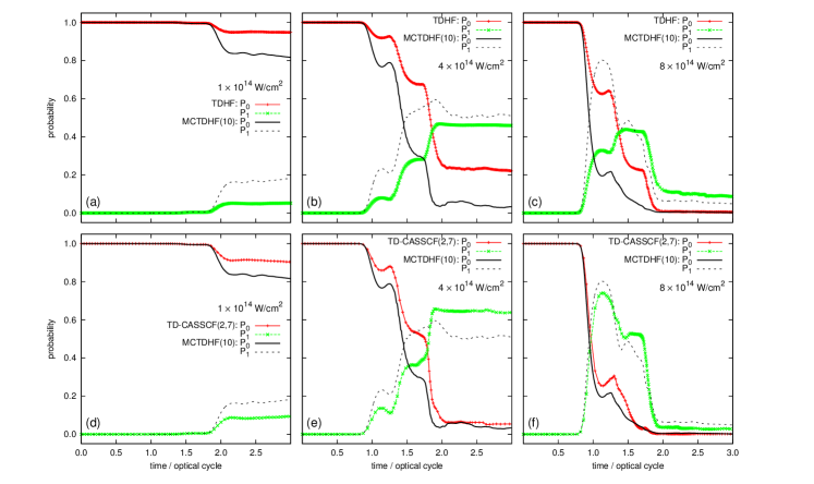
Figure 8: Ionization probabilities $P_{0}$ and $P_{1}$ of the 1D-(LiH)₂ model as a function of time, with peak intensities 1$\times$10¹⁴ (left), 4$\times$10¹⁴ (center), and 8$\times$10¹⁴ W/cm² (right). Results of TDHF (top) and TD-CASSCF($2,7$) (bottom) are compared with those of MCTDHF (black solid and dotted).

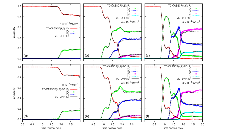
Figure 9: Ionization probabilities $P_{n}$ with $n\leq 4$ of the 1D-(LiH)₂ model as a function of time, with peak intensities 1$\times$10¹⁴ (left), 4$\times$10¹⁴ (center), and 8$\times$10¹⁴ W/cm² (right). Results of TD-CASSCF($4,8$) (top) and TD-CASSCF($4,8$)-FC (bottom) are compared with those of MCTDHF (black solid).

III.4 Analyses of computational cost

Table 2 summarizes computational times for simulations of the 1D-(LiH)₂ model with a peak intensity 4$\times$10¹⁴ W/cm². To highlight the different computational bottlenecks discussed in Sec. II.4, several box sizes ($N_{b}$ = 1000, 2000, and 3000) are considered. The CPU times in table 2-(a), (b), and (c) are recorded on a single Xeon processor of clock frequency 3.33 GHz for propagating 1000 time-steps during $2T\leq t\leq 2.1T$ with the fixed step-size RK4 algorithm, where $T=2\pi/\omega$. Entry (d) compares wall clock times spent for completing the simulation up to four optical cycles ($0\leq t\leq 4T$), with the VRK5 algorithm, measured for multi-threaded computations using 12 processors.

First, as seen in table 2-(a), CPU times for procedure (A) grows rapidly with increasing CI dimension, reproducing the theoretical linear dependence on $N_{\rm det}$. These timings marginally depend on $N_{b}$. Next, CPU times for procedure (B) in table 2-(b) scale as $O(N^{d}_{b})$ with $d$ = 1.95, 1.67, 1.66, and 1.47 for TDHF, TD-CASSCF($2,7$), TD-CASSCF($4,8$), and MCTDHF($10$) methods, respectively. This is the consequence of competing $O(n^{2}N^{2}_{b})$ and $O(n^{4}_{\rm A}N_{b})$ contributions as discussed in Sec. II.4, with growing importance of the latter for larger active spaces. The TD-CASSCF($4,8$)-FC demands less CPU times than the TD-CASSCF($4,8$), due to the strict locality of frozen-core orbitals, limiting the range of exchange operators $\hat{K}_{i}|\phi_{t}\rangle$ around the core region.

Net CPU times are listed in table 2-(c). In TDHF and TD-CASSCF calculations with core subspaces, the grid-intensive procedure (B) is definitely rate-limiting. In contrast, MCTDHF calculations involve severe bottlenecks both in procedures (A) and (B). The $N_{\rm det}$-dependent works dominate 85%, 67%, and 55% of the net CPU times, with $N_{b}$ = 1000, 2000, and 3000, respectively. The cost reduction achieved by the TD-CASSCF method largely depends on the relative importance of procedures (A) and (B). Ratios of net CPU times for TD-CASSCF($4,8$) and MCTDHF($10$) calculations are 0.12, 0.29, and 0.45 with $N_{b}$ = 1000, 2000, 3000, respectively. Similar trends are observed for wall clock times with VRK5 algorithm, as seen in table 2-(d). The stability of EOMs is found to be similar for the tested methods, requiring about 70000 evaluations of EOMs. The cost gain by the TD-CASSCF method relative to the MCTDHF method will be more drastic if $N_{\rm A}\ll N$. However, an efficient implementation of the mean field potential [Eq. (31)] is essential to achieve further speed-up for large $N_{b}$, especially in three-dimensional applications.

Table 2: Computational times for simulations of the 1D-(LiH)₂ model. First row: Numbers of determinant $N_{\rm det}$ within the symmetry of zero spin projection. Entries (a), (b), and (c): Central processor unit (CPU) times in minutes for (A), (B), and overall procedures defined in Sec. II.4, respectively. Entry (d): Wall clock times in minutes spent to complete the propagation of four optical cycles. Different simulation boxes are employed: $L=200$ ($N_{b}=1000$), $L=400$ ($N_{b}=2000$), and $L=600$ ($N_{b}=3000$). See text for more details.

	TDHF	TD-CASSCF			MCTDHF
active space	(0,0)	(2,7)	(4,8)	(4,8)-FC	(8,10)
$N_{\rm det}$	$1$	$49$	$784$	$784$	$44100$
(a) RK4 / 1000 steps, CPU-A
$N_{b}$ = $1000$	$0.0$	$0.1$	$1.2$	$1.2$	$212.4$
$N_{b}$ = $2000$	$0.0$	$0.2$	$1.3$	$1.3$	$215.1$
$N_{b}$ = $3000$	$0.0$	$0.3$	$1.4$	$1.4$	$215.3$
(b) RK4 / 1000 steps, CPU-B
$N_{b}$ = $1000$	$4.3$	$26.8$	$28.4$	$22.0$	$35.7$
$N_{b}$ = $2000$	$16.3$	$87.6$	$90.9$	$73.8$	$103.5$
$N_{b}$ = $3000$	$36.8$	$168.0$	$175.4$	$132.9$	$177.2$
(c) RK4 / 1000 steps, CPU net
$N_{b}$ = $1000$	$4.4$	$27.0$	$29.8$	$23.4$	$248.9$
$N_{b}$ = $2000$	$16.4$	$88.1$	$92.5$	$75.4$	$319.4$
$N_{b}$ = $3000$	$36.9$	$168.7$	$177.3$	$134.7$	$393.5$
(d) VRK5 / 4 cycles, Wall
$N_{b}$ = $1000$	$8.2$	$43.7$	$51.3$	$39.1$	$451.5$
$N_{b}$ = $2000$	$31.0$	$174.8$	$192.6$	$141.4$	$628.8$
$N_{b}$ = $3000$	$65.2$	$378.5$	$394.0$	$282.9$	$823.1$

IV Conclusions

We have developed a new ab initio time-dependent many-electron method called TD-CASSCF. It applies the concept of CASSCF, which has been developed for the electronic structure calculation in quantum chemistry, to the multielectron dynamics in intense laser fields, introducing frozen-core, dynamical-core, and active orbital subspaces. The classification into the subspaces can be done flexibly conforming to simulated physical situations and desired accuracy, and both TDHF and MCTDHF methods are included as special cases. This feature enables compact yet accurate representation of ionization dynamics in many-electron systems, and bridge the huge gap between TDHF and MCTDHF methods.

We have applied the TD-CASSCF method to the ionization dynamics of 1D-LiH and 1D-(LiH)₂, to assess its capability to describe multichannel and multielectron ionization. It has been confirmed that the present method closely reproduces rigorous MCTDHF results if the active orbital space is properly chosen to include appreciably ionizing electrons. We have also confirmed that the TD-CASSCF provides substantial computational cost reduction in the CI-length dependent procedures, which scale by far the steepest with the system size in the MCTDHF method. Therefore, the TD-CASSCF method is most advantageous for problems in which only a few weakly-bound electrons out of a large number of total electrons ionize.

While it is sometimes stated that the MCTDHF method is a time-dependent version of the CASSCF method Nest et al. (2005); Nest and Klamroth (2005), this statement is even more suitable for the TD-CASSCF method introduced in the present study. With reduced computational cost, the TD-CASSCF method with a properly chosen active space preserves most of the theoretically important properties of the MCTDHF: (i) flexibility to account for the strong-correlation involved in the ionization dynamics, (ii) size-extensivity, essential for a balanced description of different electronic configurations, (iii) gauge-invariance by virtue of the time-dependent variational optimization of orbitals, and (iv) invariance against orbital transformation within an orbital subspace, allowing e.g., the natural orbital analyses of the time-dependent wavefunction Kato and Kono (2009).

It should be noted that the computational cost of the TD-CASSCF method still scales factorially with the number of active (not total) electrons, thus its applications are limited to, say, 16 half-filled active orbitals in view of the present state of the art in quantum chemistry. An example requiring such a large active space is the ionization from densely lying multiple valence orbitals in weakly-interacting molecular clusters. To approach to such a problem, more restricted (instead of complete) constructions of the active space will be necessary. Moreover, a breakthrough is needed to represent one-particle wavefunctions in the general molecular potential without particular symmetries. In spite of these challenges, we foresee that the TD-CASSCF method will find fruitful applications in multielectron dynamics of, e.g., rare gas atoms heavier than helium, or molecules composed of atoms in the first few rows of the periodic table, exposed to visible-to-mid-infrared high-intensity pulses, which are inaccessible with the all-electron-active MCTDHF method.

Appendix A Calculation of ionization probabilities

To conveniently evaluate the multiple ionization yield in many electron systems, we introduce a domain-based ionization probability $P_{n}$, defined as a probability to find $n$ electrons in the outer region $|\bm{r}|>R_{\rm ion}$ and the remaining $N-n$ electrons in the inner region $|\bm{r}|<R_{\rm ion}$, with a given distance $R$ from the origin,

$$P_{n} \equiv \binom{N}{n}\int_{>}dx_{1}\cdot\cdot\int_{>}dx_{n}\int_{<}dx_{n+1}\cdot\cdot\int_{<}dx_{N}$$ (59)

$$\Psi^{*}(x_{1},\cdot\cdot,x_{N})*\Psi(x_{1},\cdot\cdot,x_{N}),$$

where $\int_{<}$ and $\int_{>}$ symbolize integrations over a spatial-spin variable $x=\{\bm{r},\xi\}$ with the spatial part restricted to the domains $|\bm{r}|<R_{\rm ion}$, and $|\bm{r}|>R_{\rm ion}$, respectively.

It is convenient to introduce an auxiliary quantity $T_{n}$ obtained by replacing the outer-region integrals in Eq. (59) with the full-region ones ($\int_{>}\rightarrow\int$). It relates to $P_{n}$ as

$$P_{n}=\sum_{k=0}^{n}\binom{N-n+k}{k}(-1)^{k}T_{n-k}.$$ (60)

By adopting the CI expansion of Eq. (8), and making use of the orthonormality of spin-orbitals in the full-space integration, we have

$$T_{n} = \sum_{IJ}^{\Pi}C^{*}_{I}C_{J}D^{(n)}_{IJ},$$ (61)

where

$$D^{(0)}_{IJ} = \sum_{ij}^{N}\det\left(S^{<}_{IJ}\right),$$

$$D^{(1)}_{IJ} = \sum_{ij}^{N}\epsilon^{IJ}_{ij}\det\left(S^{<}_{IJ}[i:j]\right),$$

$$D^{(2)}_{IJ} = \sum_{i>j}^{N}\sum_{k>l}^{N}\epsilon^{IJ}_{ik}\epsilon^{IJ}_{jl}\det\left(S^{<}_{IJ}[ij:kl]\right),$$ (62)

etc, and $S^{<}_{IJ}$ is an $N\times N$ matrix with its $\{ij\}$ element being the inner-region overlap integral,

$$(S^{<}_{IJ})_{ij}=\int_{<}dx\phi^{*}_{p(i,I)}(x)\phi_{q(j,J)}(x)\equiv\langle\phi_{p}|\phi_{q}\rangle_{<},$$ (63)

with $\phi_{p(i,I)}$ being the $i$-th (in a predefined order) spin-orbital in the determinant $I$. $S^{<}_{IJ}[ij\cdot\cdot:kl\cdot\cdot]$ is the submatrix of $S^{<}_{IJ}$ obtained after removing rows $i,j,\cdot\cdot$ and columns $k,l,\cdot\cdot$ from the latter, and

$$\epsilon^{IJ}_{ij}=\delta^{p(i,I)}_{q(j,J)}(-1)^{i+j}.$$ (64)

The matrix $S^{<}_{IJ}$ and its submatrices are block-diagonal due to the spin-orthonormality, so that, e.g., $\det\left(S^{<}_{IJ}\right)=\det\left(S^{<}_{I^{\alpha}J^{\alpha}}\right)\det\left(S^{<}_{I^{\beta}J^{\beta}}\right)$, where $I^{\sigma}$ is the $\sigma$-spin part of the determinant $I$.

The procedure given above remains a manageable task in the present applications, up to eight (all) electron ionization probabilities in the 1D-(LiH)₂ model. While this scheme becomes impractical for systems with more electrons, it may still be useful for problems where only a few electrons are ejected appreciably, since the dimension of Eqs. (A) can be reduced to the number of the ionizing electrons.

This approach allows the evaluation of multiple ionization yields by using the information of the inner region orbitals $\langle\phi_{p}|\phi_{q}\rangle_{<}$ and the formal orthonormality relation $\delta^{p}_{q}=\langle\phi_{p}|\phi_{q}\rangle_{<}+\langle\phi_{p}|\phi_{q}\rangle_{>}$. It works with a reasonable size of the simulation box $L$, provided that $R_{\rm ion}\ll L$ and a good absorber is implemented to prevent the reflection of the wavefunction. In fact, we performed calculations for the 1D-(LiH)₂ model in Sec. III using smaller boxes with $L$ = 200 and 400 a.u., where a sizable portion of the norm is lost at the boundary, and confirmed that the obtained ionization yields are virtually the same with those of Fig. 8 and 9. Such small-scale calculations could serve as preliminary validations for the choice of the active space before stepping into large-scale computations.

References

- Strickland and Mourou (1985) D. Strickland and G. Mourou, Opt. Commun. 56, 219 (1985).
- Bahk et al. (2004) S.-W. Bahk, P. Rousseau, T. A. Planchon, V. Chvykov, G. Kalintchenko, A. Maksimchuk, G. A. Mourou, and V. Yanovsky, Opt. Lett. 29, 2837 (2004).
- Yanovsky et al. (2008) V. Yanovsky, V. Chvykov, G. Kalinchenko, P. Rousseau, T. Planchon, T. Matsuoka, A. Maksimchuk, J. Nees, G. Cheriaux, G. Mourou, and K. Krushelnick, Opt. Express 16, 2109 (2008).
- Yu et al. (2012) T. J. Yu, S. K. Lee, J. H. Sung, J. W. Yoon, T. M. Jeong, and J. Lee, Opt. Express 20, 10807 (2012).
- Protopapas et al. (1997) M. Protopapas, C. H. Keitel, and P. L. Knight, Rep. Prog. Phys. 60, 389 (1997).
- Brabec and Krausz (2000) T. Brabec and F. Krausz, Rev. Mod. Phys. 72, 545 (2000).
- Seres et al. (2005) J. Seres, E. Seres, A. J. Verhoef, G. Tempea, C. Streli, P. Wobrauschek, V. Yakovlev, A. Scrinzi, C. Spielmann, and F. Krausz, Nature 433, 596 (2005).
- Chang (2011) Z. Chang, Fundamentals of Attosecond Optics (CRC, Boca Raton, 2011).
- Itatani et al. (2004) J. Itatani, J. Levesque, D. Zeidler, H. Niikura, H. Pèpin, J. C. Kieffer, P. B. Corkum, and D. M. Villeneuve, Nature 432, 867 (2004).
- Haessler et al. (2010) S. Haessler, J. Caillat, W. Boutu, C. Giovanetti-Teixeira, T. Ruchon, T. Auguste, Z. Diveki, P. Breger, A. Maquet, B. Carré, R. Taïeb, and P. Salières, Nature Phys. 6, 200 (2010).
- Salières et al. (2012) P. Salières, A. Maquet, S. Haessler, J. Caillat, and R. Taïeb, Rep. Prog. Phys. 75, 062401 (2012).
- Agostini and DiMauro (2004) P. Agostini and L. F. DiMauro, Rep. Prog. Phys. 67, 813 (2004).
- Krausz and Ivanov (2009) F. Krausz and M. Ivanov, Rev. Mod. Phys. 81, 163 (2009).
- Gallmann et al. (2013) L. Gallmann, C. Cirelli, and U. Keller, Annu. Rev. Phys. Chem. 63, 447 (2013).
- Sekikawa et al. (2004) T. Sekikawa, A. Kosuge, T. Kanai, and S. Watanabe, Nature (London) 432, 605 (2004).
- Nabekawa et al. (2005) Y. Nabekawa, H. Hasegawa, E. J. Takahashi, and K. Midorikawa, Phys. Rev. Lett. 94, 043001 (2005).
- Pindzola and Robicheaux (1998a) M. S. Pindzola and F. Robicheaux, Phys. Rev. A 57, 318 (1998a).
- Pindzola and Robicheaux (1998b) M. S. Pindzola and F. Robicheaux, J. Phys. B 31, L823 (1998b).
- Colgan et al. (2001) J. Colgan, M. S. Pindzola, and F. Robicheaux, J. Phys. B 34, L457 (2001).
- Parker et al. (2001) J. S. Parker, L. R. Moore, K. J. Meharg, D. Dundas, and K. T. Taylor, J. Phys. B 34, L69 (2001).
- Laulan and Bachau (2003) S. Laulan and H. Bachau, Phys. Rev. A 68, 013409 (2003).
- Piraux et al. (2003) B. Piraux, J. Bauer, S. Laulan, and H. Bachau, Eur. Phys. J. D 26, 7 (2003).
- Laulan and Bachau (2004) S. Laulan and H. Bachau, Phys. Rev. A 69, 033408 (2004).
- Ishikawa and Midorikawa (2005) K. L. Ishikawa and K. Midorikawa, Phys. Rev. A 72, 013407 (2005).
- Feist et al. (2009) J. Feist, S. Nagele, R. Pazourek, E. Persson, B. I. Schneider, L. A. Collins, and J. Burgdörfer, Phys. Rev. Lett. 103, 063002 (2009).
- Pazourek et al. (2011) R. Pazourek, J. Feist, S. Nagele, E. Persson, B. I. Schneider, L. A. Collins, and J. Burgdörfer, Phys. Rev. A 83, 053418 (2011).
- Ishikawa and Ueda (2012) K. L. Ishikawa and K. Ueda, Phys. Rev. Lett. 108, 033003 (2012).
- Sukiasyan et al. (2012) S. Sukiasyan, K. L. Ishikawa, and M. Ivanov, Phys. Rev. A 86, 033423 (2012).
- Ishikawa and Ueda (2013) K. L. Ishikawa and K. Ueda, Appl. Sci. 3, 189 (2013).
- Vanroose et al. (2006) W. Vanroose, D. A. Horner, F. Martín, T. N. Rescigno, and C. W. McCurdy, Phys. Rev. A 74, 052702 (2006).
- Horner et al. (2008) D. A. Horner, S. Miyabe, T. N. Rescigno, C. W. McCurdy, F. Morales, and F. Martín, Phys. Rev. Lett. 101, 183002 (2008).
- Lee et al. (2010) T.-G. Lee, M. S. Pindzola, and F. Robicheaux, J. Phys. B 43, 165601 (2010).
- Gordon et al. (2006) A. Gordon, F. X. Kärtner, N. Rohringer, and R. Santra, Phys. Rev. Lett. 96, 223902 (2006).
- Rohringer and Santra (2009) N. Rohringer and R. Santra, Phys. Rev. A 79, 053402 (2009).
- Smirnova et al. (2009) O. Smirnova, S. Patchkovskii, Y. Mairesse, N. Dudovich, and M. Y. Ivanov, Proc. Natl. Acad. Sci. 106, 16556 (2009).
- Akagi et al. (2009) H. Akagi, T. Otobe, A. Staudte, A. Shiner, F. Turner, R. Dörner, D. M. Villeneuve, and P. B. Corkum, Science 325, 1364 (2009).
- Boguslavskiy et al. (2012) A. E. Boguslavskiy, J. Mikosch, A. Gijsbertsen, M. Spanner, S. Patchkovskii, N. Gador, M. J. J. Vrakking, and A. Stolow, Science 335, 1336 (2012).
- Caillat et al. (2005) J. Caillat, J. Zanghellini, M. Kitzler, O. Koch, W. Kreuzer, and A. Scrinzi, Phys. Rev. A 71, 012712 (2005).
- Rohringer et al. (2006) N. Rohringer, A. Gordon, and R. Santra, Phys. Rev. A 74, 043420 (2006).
- Greenman et al. (2010) L. Greenman, P. J. Ho, S. Pabst, E. Kamarchik, D. A. Mazziotti, and R. Santra, Phys. Rev. A 82, 023406 (2010).
- Gross et al. (1996) E. K. U. Gross, J. F. Dobson, and M. Petersilka, Top. Curr. Chem. 181, 81 (1996).
- Otobe et al. (2004) T. Otobe, K. Yabana, and J.-I. Iwata, Phys. Rev. A 69, 053404 (2004).
- Telnov and Chu (2009) D. A. Telnov and S.-I. Chu, Phys. Rev. A 80, 043412 (2009).
- Kvaal (2012) S. Kvaal, J. Chem. Phys. 136, 194109 (2012).
- Huber and Klamroth (2011) C. Huber and T. Klamroth, J. Chem. Phys. 134, 054113 (2011).
- Hochstuhl and Bonitz (2012) D. Hochstuhl and M. Bonitz, Phys. Rev. A 86, 053424 (2012).
- Olsen et al. (1988) J. Olsen, B. O. Roos, P. Jørgensen, and H. J. A. Jensen, J. Chem. Phys. 89, 2185 (1988).
- Szabo and Ostlund (1996) A. Szabo and N. S. Ostlund, Modern Quantum Chemistry (Dover, Mineola, 1996).
- Helgaker et al. (2002) T. Helgaker, P. Jørgensen, and J. Olsen, Molecular Electronic-Structure Theory (Wiley, 2002).
- Ruedenberg et al. (1982) K. Ruedenberg, M. W. Schmidt, M. M. Gilbert, and S. T. Elbert, Chem. Phys. 71, 41 (1982).
- Roos et al. (1980) B. O. Roos, P. R. Taylor, and P. E. M. Siegbahn, Chem. Phys. 48, 157 (1980).
- Roos (1987) B. O. Roos, Adv. Chem. Phys. 69, 399 (1987).
- Schmidt and Gordon (1998) M. W. Schmidt and M. S. Gordon, Annu. Rev. Phys. Chem. 49, 233 (1998).
- Pindzola et al. (1991) M. S. Pindzola, D. C. Griffin, and C. Bottcher, Phys. Rev. Lett. 66, 2305 (1991).
- Pindzola et al. (1997) M. S. Pindzola, F. Robicheaux, and P. Gavras, Phys. Rev. A 55, 1307 (1997).
- Tolley (1999) A. J. Tolley, J. Phys. B 32, 3449 (1999).
- Dahlen and van Leeuwen (2001) N. E. Dahlen and R. van Leeuwen, Phys. Rev. A 64, 023405 (2001).
- Nguyen and Bandrauk (2006) N. A. Nguyen and A. D. Bandrauk, Phys. Rev. A 73, 032708 (2006).
- Kato and Kono (2004) T. Kato and H. Kono, Chem. Phys. Lett. 392, 533 (2004).
- Nest et al. (2005) M. Nest, T. Klamroth, and P. Saalfrank, J. Chem. Phys. 122, 124102 (2005).
- Nest and Klamroth (2005) M. Nest and T. Klamroth, Phys. Rev. A 72, 012710 (2005).
- Jordan et al. (2006) G. Jordan, J. Caillat, C. Ede, and A. Scrinzi, J. Phys. B 39, S341 (2006).
- Kato and Kono (2008) T. Kato and H. Kono, J. Chem. Phys. 128, 184102 (2008).
- Alon et al. (2007) O. E. Alon, A. I. Streltsov, and L. S. Cederbaum, J. Chem. Phys. 127, 154103 (2007).
- Hochstuhl and Bonitz (2011) D. Hochstuhl and M. Bonitz, J. Chem. Phys. 134, 084106 (2011).
- Miranda et al. (2011) R. P. Miranda, A. J. Fisher, L. Stella, and A. P. Horsfield, J. Chem. Phys. 134, 244101 (2011).
- Beck et al. (2000) M. H. Beck, A. Jäckle, G. A. Worth, and H.-D. Meyer, Phys. Rep. 324, 1 (2000).
- Li et al. (2005) X. Li, S. M. Smith, A. N. Markevitch, D. A. Romanov, R. J. Levis, and H. B. Schlegel, Phys. Chem. Chem. Phys. 7, 233 (2005).
- Frenkel (1934) J. Frenkel, Wave Mechanics-Advanced General Theory (Oxford at the Clarendon Press, 1934).
- Lwdin and Mukherjee (1972) P.-O. Lwdin and P. K. Mukherjee, Chem. Phys. Lett. 14, 1 (1972).
- Moccia (1973) R. Moccia, Int. J. Quantum Chem. 7, 779 (1973).
- (72) H. Miyagi and L. B. Madsen, unpublished .
- Levy and Berthier (1968) B. Levy and G. Berthier, Int. J. Quantum Chem. 2, 307 (1968).
- Levy and Berthier (1969) B. Levy and G. Berthier, Int. J. Quantum Chem. 3, 247 (1969).
- Balzer et al. (2010a) K. Balzer, S. Bauch, and M. Bonitz, Phys. Rev. A 81, 022510 (2010a).
- Balzer et al. (2010b) K. Balzer, S. Bauch, and M. Bonitz, Phys. Rev. A 82, 033427 (2010b).
- Kutzelnigg (1963) W. Kutzelnigg, Theoret. Chim. Acta. 1, 327 (1963).
- Kutzelnigg (1964) W. Kutzelnigg, J. Chem. Phys. 40, 3640 (1964).
- Kato and Kono (2009) T. Kato and H. Kono, Chem. Phys. 366, 46 (2009).