An Efficient MAC Protocol with Selective Grouping and Cooperative Sensing in Cognitive Radio Networks

Abstract

In cognitive radio networks, spectrum sensing is a crucial technique to discover spectrum opportunities for the Secondary Users (SUs). The quality of spectrum sensing is evaluated by both sensing accuracy and sensing efficiency. Here, sensing accuracy is represented by the false alarm probability and the detection probability while sensing efficiency is represented by the sensing overhead and network throughput. In this paper, we propose a group-based cooperative Medium Access Control (MAC) protocol called GC-MAC, which addresses the tradeoff between sensing accuracy and efficiency. In GC-MAC, the cooperative SUs are grouped into several teams. During a sensing period, each team senses a different channel while SUs in the same team perform the joint detection on the targeted channel. The sensing process will not stop unless an available channel is discovered. To reduce the sensing overhead, an SU-selecting algorithm is presented to selectively choose the cooperative SUs based on the channel dynamics and usage patterns. Then, an analytical model is built to study the sensing accuracy-efficiency tradeoff under two types of channel conditions: time-invariant channel and time-varying channel. An optimization problem that maximizes achievable throughput is formulated to optimize the important design parameters. Both saturation and non-saturation situations are investigated with respect to throughput and sensing overhead. Simulation results indicate that the proposed protocol is able to significantly decrease sensing overhead and increase network throughput with guaranteed sensing accuracy.

I Introduction

Recently, the explosive increase of wireless devices and applications poses a serious problem of compelling need of numerous radio spectrum. The problem is greatly caused by the current fixed frequency allocation policy, which allocates a fixed frequency band to a specific wireless system. On the contrary, a recent report published by the Federal Communication Commission (FCC) reveals that most of the licensed spectrum is rarely utilized continuously across time and space [1]. In order to address the spectrum scarcity and the spectrum under-utilization, Cognitive Radio (CR) has been proposed to effectively utilize the spectrum [2]-[4]. In the CR networks, the Secondary (unlicensed) Users (SUs) are allowed to opportunistically operate in the frequency bands originally allocated to the Primary (licensed) Users (PUs) when the bands are not occupied by PUs. SUs are capable to sense unused bands and adjust transmission parameters accordingly, which makes CR an excellent candidate technology for improving spectrum utilization.

Spectrum sensing is a fundamental technology for SUs to efficiently and accurately detect PUs in order to avoid the interference to primary networks. However, in CR networks, many unreliable conditions [6]-[8], such as channel uncertainty, noise uncertainty and no knowledge of primary signals, will degrade the performance of spectrum sensing. Cooperative sensing [9]-[15], has been studied extensively as a promising alternative to improve sensing performance at both of the physical (PHY) level and the medium access control (MAC) level. The main interest of this paper is the cooperative sensing mechanism at the MAC level, which performs sensing operations in two aspects: 1) assign multiple SUs to sense a single channel for improving the sensing accuracy; 2) assign cooperative SUs to search for available spectrums in parallel to enhance sensing efficiency.

The improvement of sensing accuracy is extensively treated in [10]-[12]. The study in [10] reports a cooperative sensing approach through multi-user cooperation and evaluates the sensing accuracy. The authors of [11] consider cooperative sensing by using a counting rule and derive optimal strategies under both the Neyman-Pearson criterion and the Bayesian criterion. The study in [12] presents a new cooperative wide-band spectrum sensing scheme that exploits the spatial diversity among multiple SUs which also contributes to improve the sensing accuracy. These studies have mainly focused on improving sensing accuracy while sensing efficiency has been ignored. The enhancement for sensing efficiency has been investigated in [13][14]. The study in [13] introduces an opportunistic multi-channel MAC protocol which integrate two novel cooperative sensing mechanisms, i.e., random sensing policy and negotiation-based sensing policy. The latter strategy assigns SUs to collaboratively sense different channels to improve the sensing efficiency. For the sake of reducing sensing overhead, the authors of [14] propose a multi-channel cooperative sensing scheme, where the cooperative SUs are optimally selected to sense the distinct channels at the same time for sensing efficiency. These works assume that the sensing accuracy of one channel by a single SU is completely true which is may not be practical in real communication systems.

In addition, literatures above did not consider the design of the cooperative MAC protocol for distributed networks and perform theoretical analysis of sensing overhead and throughput. Hence, we are interested in achieving both sensing accuracy and sensing efficiency by introducing a cooperation protocol in MAC layer for CR networks. Several cognitive MAC protocols have been proposed in the literature to address various issues in CR network [13][17][20]-[25]. However, these protocols do not leverage the benefit of cooperation at MAC layer for enhancing the sensing efficiency without degrading the sensing accuracy.

In this paper, we propose a group-based cooperative MAC protocol called GC-MAC. In GC-MAC, the cooperative SUs are grouped into several teams. During a sensing period, each team senses a different channel. The sensing process will not stop unless an available spectrum channel is discovered. The purpose of team division has twofold: 1) sensing a channel by several SUs for the improvement of sensing accuracy; 2) finding more spectrum opportunities by sensing distinct channels by different teams. As a consequence, multiple distinct channels can be simultaneously detected within one sensing period which leads to the enhancement of sensing efficiency.

To reduce the sensing overhead, we propose an SU-selecting algorithm for GC-MAC protocol. In the SU-selecting algorithm, we selectively choose the optimal number of the cooperative SUs for each team based on the channel occupation dynamics in order to substantially reduce sensing overhead. We analyze the sensing overhead and throughput in the saturation and no-saturation network cases, respectively. In the saturation networks, each SU always has data to transmit. In the non-saturation networks, an SU may have an empty queue. In every network case, we consider two types of channel conditions: time-invariant channel and time-varying channel. In each condition, the sensing overhead and the throughput are incorporated into an achievable throughput maximization problem, which is formulated to find the key design parameters: the number of the cooperative teams and the number of SUs in one team. Furthermore, we present extensive examples to demonstrate the sensing efficiency comparing with the existing schemes and to show the determination of the crucial parameters. Simulation results demonstrate that our proposed scheme is able to achieve substantially higher throughput and lower sensing overhead, comparing to existing mechanisms.

The remainder of this paper is organized as follows. In Section II, the system models are introduced. Section III reports our proposed group-based MAC protocols for cooperative CR network. Section IV introduces an SU-selecting algorithm for appropriately selecting the cooperative SUs so as to reduce the sensing overhead. Then, we study the sensing overhead and achievable throughput in the saturation and non-saturation networks in Section V and Section VI, respectively. Section VII evaluates the performance of the proposed GC-MAC protocol based on our developed analytical models. Finally, we draw our conclusions in Section VIII.

II Systems Models

II-A Channel Usage Model

We assume that each licensed channel alternates between ON and OFF state, of which the OFF time is not used by PUs and hence can be exploited by the SUs. Assume that the durations of the ON and the OFF period are independently exponentially distributed. For a given licensed channel, the duration of ON period follows an exponentially distributed with parameter $\mu_{ON}$ and the duration of OFF period with an exponentially distributed parameter $\mu_{OFF}$. We define the channel availability as the normalized period which is available for SUs. Let $p$ denotes the channel availability. Then, we have $p=\frac{\mu_{ON}}{\mu_{OFF}+\mu_{ON}}$. Similar to [13], in this paper, we mainly consider that the licensed channels used by the same set of PUs, i.e., the licensed channel availability information sensed by each SUs is consistent among all SUs.

We consider two scenarios depending on the channel dynamics. The first is the time-invariant channel with unchanged channel date rate $R$. The throughput of the SU by using time-invariant channel only depends on the constant data rate and the valid transmission time $T_{r}$. The second type of channel is the Time-Varying Channel. The Finite-State Markov Channel (FSMC) model is employed to model the dynamics of the time-varying channel [19]. The dynamics of the time-varying channel is partitioned based on the channel data rate. It is reasonable to employ the channel data rate instead of Signal-to-Noise Ratio (SNR) which has been used in conventional FSMC model. Since the channel data rate is closely relevant to the application layer requirements and hence its usage facilitates the construction of resource demands from an application perspective. The set of the channel state is denoted as $\mathbf{M}\equiv\{1,2,\dots,M\}$ with $\mid\!\mathbf{M}\!\mid=M$. Let $c_{i}$ represents the channel state $i$ $(i\in\mathbf{M})$. The state space is denoted as $\mathbf{S}\equiv\{c_{i},i\in\mathbf{M}\}$. Let $\pi_{i}$ $(i\in\mathbf{M})$ represents the steady-state probability at state $c_{i}$. Then, the steady-state probability can be solved using the similar technique in [19]. During data transmission within a frame, the time-variation is slow enough that the channel data rate does not change substantially. This assumption is acceptable due to the short data transmission period within a frame and has been frequently used, e.g. [18] [26].

II-B Energy Detection Model

In order to discuss our problem, we employ Energy Detection [27] as the spectrum sensing scheme. Both of the real-valued signal model and the complex-valued signal model are used to describe the received signal at the SU’s receiver.

II-B1 Real-Valued Signal Model

Let $t_{s}$ be the sensing time and $f_{s}$ be the sample frequency during sensing time. We denotes $N$ as the number of samples in a sensing period, i.e. $N=t_{s}f_{s}$. The received signal $r_{k}(n)$ at the $n$th sample and the $k$th SU is given by,

$$r_{k}(n)=\left\{\begin{array}[]{l}w_{k}(n),\quad\quad\quad\quad H_{0}\\ s_{k}(n)+w_{k}(n),\quad H_{1}\end{array}\right.$$

where $H_{0}$ represents the hypothesis that PUs are absent, and $H_{1}$ represents the hypothesis that PUs are present. $s_{k}(n)$ represents the PU’s transmitted signal which is assumed as a real-valued Gaussian signal with mean zero and variance $\sigma_{s}^{2}$. $w_{k}(n)$ denotes a Gaussian process with mean zero and variance $\sigma_{w}^{2}$.

Let $e_{k}(r)$ denotes the test statistic of the $k$th SU. Then, we have $e_{k}(r)=\sum_{n=1}^{N}\mid r_{k}(n)\mid^{2}$. The detection and false alarm probability of $k$th SU are given by,

$$P_{d}^{k}=Pr\left[e_{k}(r)>\lambda\mid H_{1}\right],\quad P_{f}^{k}=Pr\left[e_{k}(r)>\lambda\mid H_{0}\right]$$

where $\lambda$ is a decision threshold of energy detector for a SU.

The test statistic $e(r)$ is known as Chi-square distribution with $\frac{e(r)}{\sigma_{w}^{2}}\sim\chi_{N}^{2}$ under hypothesis $H_{0}$, and $\frac{e(r)}{\sigma_{s}^{2}+\sigma_{w}^{2}}\sim\chi_{N}^{2}$ under hypothesis $H_{1}$. However, if the number of samples is large, we can use the Central Limit Theorem (CLT) to approximate the Chi-square distribution by Gaussian distribution [27] under hypothesis $H_{z}(z=0,1)$ with mean $\mu_{z}$ and variance $\sigma_{z}^{2}$ as,

$$\left\{\begin{array}[]{l}\mu_{0}=N\sigma_{w}^{2},\quad\quad\quad\quad\quad\sigma_{0}^{2}=2N\sigma_{w}^{4},\quad\quad\quad\quad\quad H_{0}\\ \mu_{1}=N(\sigma_{s}^{2}+\sigma_{w}^{2}),\quad\quad\sigma_{1}^{2}=2N(\sigma_{s}^{2}+\sigma_{w}^{2})^{2},\quad H_{1}.\end{array}\right.$$

Therefore, the probabilities $P_{d}^{k}$ and $P_{f}^{k}$ can be approximated in terms of the $Q$ function is given by,

$$P_{d}^{k}=Q\left(\frac{\lambda-N(\sigma_{s}^{2}+\sigma_{w}^{2})}{\sqrt{2N}(\sigma_{s}^{2}+\sigma_{w}^{2})}\right),\quad P_{f}^{k}=Q\left(\frac{\lambda-N\sigma_{w}^{2}}{\sqrt{2N}\sigma_{w}^{2}}\right)$$

where $Q(x)=\frac{1}{\sqrt{2\pi}}\int_{x}^{\infty}e^{(-\frac{t^{2}}{2})}dt$.

II-B2 Complex-Valued Signal Model

Considering the complex-valued signal model, the received signal $r_{k}(n)$ at the $n$th sample and the $k$th SU can be given by,

$$r_{k}(n)=\left\{\begin{array}[]{l}w_{k}(n),\quad\quad\quad\quad H_{0}\\ h_{k}s_{k}(n)+w_{k}(n),\quad H_{1}\end{array}\right.$$

where the channel coefficients $h_{k}$ is zero-mean, unit-variance complex Gaussian random variables. $s_{k}(n)$ represents the PU’s transmitted signal which is assumed as a Gaussian signal with mean zero and variance $\sigma_{s}^{2}$. $w_{k}(n)$ denotes a Gaussian process with mean zero and variance $\sigma_{w}^{2}$.

The test statistic of the $k$th SU $e_{k}(r)=\sum_{n=1}^{N}\mid r_{k}(n)\mid^{2}$. The detection and false alarm probability of $k$th SU are given by,

$$P_{d}^{k}=Pr\left[e_{k}(r)>\lambda_{c}\mid H_{1}\right],\quad P_{f}^{k}=Pr\left[e_{k}(r)>\lambda_{c}\mid H_{0}\right],$$

where $\lambda_{c}$ is a decision threshold of energy detector for a single SU considering the complex-valued signal model. For a large $N$, the distribution of $e_{k}(r)$ can be approximated as Gaussian distribution [27] with mean $\mu_{z}$ and variance $\sigma_{z}^{2}$ under hypothesis $H_{z}(z=0,1)$ as,

$$\left\{\begin{array}[]{l}\mu_{0}=N\sigma_{w}^{2},\quad\quad\quad\quad\quad\quad\quad\sigma_{0}^{2}=2N\sigma_{w}^{4},\quad\quad\quad\quad\quad\quad H_{0}\\ \mu_{1}=N(\mid h_{k}\mid^{2}\sigma_{s}^{2}+\sigma_{w}^{2}),\quad\sigma_{1}^{2}=2N(\mid h_{k}\mid^{2}\sigma_{s}^{2}+\sigma_{w}^{2})^{2},H_{1}\end{array}\right.$$

Finally, we can obtain the probabilities $P_{d}^{k}$ and $P_{f}^{k}$ in terms of the $Q$ function as

$$P_{d}^{k}=Q\left(\frac{\lambda-N(\mid h_{k}\mid^{2}\sigma_{s}^{2}+\sigma_{w}^{2})}{\sqrt{2N}(\mid h_{k}\mid^{2}\sigma_{s}^{2}+\sigma_{w}^{2})}\right),P_{f}^{k}=Q\left(\frac{\lambda-N\sigma_{w}^{2}}{\sqrt{2N}\sigma_{w}^{2}}\right),$$

where $Q(x)=\frac{1}{\sqrt{2\pi}}\int_{x}^{\infty}e^{(-\frac{t^{2}}{2})}dt$.

II-C Counting Rule

In order to improve sensing performance, an efficient fusion rule is needed to make final decision to the availability of the channel. Depending on every SUs’ individual decision from one team, there are three popular fusion rules: And-rule, OR-rule and Majority-rule [18]. And-rule mainly focuses on maximizing the discovery of spectrum opportunities which are deemed to be exist if only one decision says there is no PU. In OR-rule, as far as limit the interference to the PU, the spectrum is assumed to be available only when all the reporting decisions declare that no PU is present. The last Majority-rule is based on majority of the individual decisions. If more than half of the decisions declare the appearance of primary user, then the final decision claims that there is a primary user. Without loss of generality, we use the Majority-rule in this paper with the assumption that all the individual decisions are independent, and supposing that $P_{d}^{k}=P_{d}$ and $P_{f}^{k}=P_{f}$ [18]. Then the joint detection probability and false alarm probability by $j$ number of SUs are given by

$$P_{d}(j)=\sum_{y=0}^{j-\lceil\frac{j}{2}\rceil}{j\choose\lceil\frac{j}{2}\rceil+y}(1-P_{d})^{j-\lceil\frac{j}{2}\rceil-y}P_{d}^{\lceil\frac{j}{2}\rceil+y},$$ (1)

$$P_{f}(j)=\sum_{y=0}^{j-\lceil\frac{j}{2}\rceil}{j\choose\lceil\frac{j}{2}\rceil+y}(1-P_{f})^{j-\lceil\frac{j}{2}\rceil-y}P_{f}^{\lceil\frac{j}{2}\rceil+y}.$$ (2)

III GC-MAC: Group-based Cooperative MAC protocol

In this section, we present the specifications of the proposed MAC protocol, together with the group-based cooperative spectrum sensing scheme and the SU-selecting algorithm. To describe our protocol conveniently, we have the following assumptions:

• Each SU is equipped with a single antenna which can not operate the sensing and transmission at the same time. According to this constraint, the sensing overhead caused by sensing is unavoidable and cannot be neglected in protocol design.

• A common control channel is available for all SUs to communicate at any time.

• An SUs can be assigned to perform cooperative sensing even when they have the packets to transmit.

A time frame of the secondary network operation is divided to three phases: reservation, sensing and transmission. All SUs are categorized into three types:

• Source SU ($SU_{s}$): an SU that has data to transmit.

• Cooperative SUs ($SU_{c}$): SUs that are selected for cooperative sensing.

• Destination SU ($SU_{d}$): an SU that receives the data packet from the source SU.

III-A Reservation

In GC-MAC, any $SU_{s}$ entering the network first try to perform a handshake with $SU_{d}$ on the control channel to reserve a data channel. This allows the $SU_{s}$ and $SU_{d}$ to switch to the chosen channel for data transmission. Here, we use R-RTS/R-CTS packets for $SU_{s}$ and $SU_{d}$ to compete the data channel with other SUs. The $SU_{s}$ will listen to control channel for a time interval $T$. If no R-RTS/R-CTS is received or time $T$ is expired, the $SU_{s}$ participates in the reservation process. Otherwise, it will defer and wait for the notification from the transmission pair or a timeout. Whenever there is at least one packet buffered in the queue, $SU_{s}$ sends reservation requirement to $SU_{d}$. Upon receiving the requirement, $SU_{d}$ will reply and other SUs overhearing these message exchanging cease their own sensing, and wait for the notification from this transmission pair or a timer expiration. When the sensing or cooperative sensing is finished, other neighboring SUs start a new round of competition for the control channel with a random backoff.

III-B Sensing

After reserving the data channel, $SU_{s}$ and $SU_{d}$ start to sense the spectrum channel. In this phase, we use S-RTS/S-CTS packets for spectrum sensing and negotiation between $SU_{s}$ and $SU_{d}$. In order to indicate the mechanism of our scheme, the C-RTS/C-CTS packets are included in the RTS/CTS model for $SU_{c}$ to acknowledge its participation. Fig. 1 shows the flowchart of the sensing procedure of the source node $SU_{s}$. Fig. 2 shows the flowchart of the sensing procedures of $SU_{c}$ and $SU_{d}$. In particular, we provide the detailed description as follows.

Source SU ($SU_{s}$)

1) $SU_{s}$ senses the channel to judge the availability of the channel. If the channel is not occupied by a PU, $SU_{s}$ sends an S-RTS packet to $SU_{d}$, including the availability information of the detected channel. Otherwise, $SU_{s}$ sends the channel unavailability information to $SU_{d}$.

2) If an S-CTS packet from $SU_{d}$ is not heard after a CTS timer, $SU_{s}$ should perform a random backoff, as if it encounters a collision. If $SU_{s}$ receives the information of channel availability from $SU_{d}$. $SU_{s}$ and $SU_{d}$ will start the transmission phase (please refer to Section III.C). If $SU_{s}$ receives the information of channel unavailability from $SU_{d}$, $SU_{s}$ will send C-RTS to the neighborhood of $SU_{c}$ and $SU_{d}$.

3) If $SU_{s}$ does not receive any feedback from $SU_{c}$, it then sends cooperation requirement again after a random backoff. If the feedback is successfully received, $SU_{s}$ counts the number of $SU_{c}$ according to the SU-selecting algorithm (please refer to Section IV). When the number of $SU_{c}$s satisfies the requirement of the cooperative sensing, $SU_{s}$ stops sending cooperation requirement to the neighborhood of $SU_{c}$ and divides the chosen $SU_{c}$s into a number of teams.

4) $SU_{s}$ sends the cooperative information to the $SU_{c}$s and then join the cooperative sensing with $SU_{c}$s. Such information includes grouping information and the specific channels.

5) Upon receiving the sensing results, $SU_{s}$ should declare the success of spectrum sensing and return to 1). Otherwise, $SU_{s}$ should perform a random backoff, and return to 4).

Cooperative SU ($SU_{c}$)

1) Upon receiving the cooperation requirement, $SU_{c}$ sends feedback to the source node $SU_{s}$ and waits for the cooperative information.

2) If the information for the cooperation is not received after a CTS timer, $SU_{c}$ assumes that the information is lost and then reverts to the original state. Otherwise, $SU_{c}$ starts the channel sensing based on the cooperative information.

3) After the time duration $t_{s}$, $SU_{c}$ determines the PU’s activity on the detected channel and sends cooperation acknowledgement to $SU_{s}$ with the sensing result.

Destination SU ($SU_{d}$)

1) $SU_{d}$ senses the same channel with $SU_{s}$ in a synchronous way. After the sensing time $t_{s}$, $SU_{d}$ makes the final decision about the state (ON/OFF) of the channel, and waits for the sensing requirement from the source node $SU_{s}$.

2) If the destination node $SU_{d}$ receives the sensing requirement with the sensing result from the source node $SU_{s}$, it delivers the sensing result back to $SU_{s}$. If the sensing result indicates that the channel is available, $SU_{d}$ is ready for receiving data. Otherwise, $SU_{d}$ waits for the cooperation requirement.

3) If cooperation requirement is received, $SU_{d}$ will join the cooperative sensing and report the sensing results to $SU_{s}$. Then, $SU_{d}$ returns to 2). If neither a sensing nor an cooperation requirement is heard after a timer, $SU_{d}$ will go back to the initial state.

Figure 1: The sensing work flow of $SU_{s}$.

Figure 2: The sensing work flow of $SU_{c}$ and $SU_{d}$.

III-C Transmission

After the source node $SU_{s}$ and the destination node $SU_{d}$ successfully find an available channel, they begin to use the channel to transmit data packets. Here, we use the T-RTS/T-CTS pair to indicate the transmission process. Before starting the transmission, $SU_{s}$ will send T-RTS to $SU_{d}$ for declaring the beginning of transmission. Upon receiving this requirement, $SU_{d}$ replies T-CTS. If this feedback is received, $SU_{s}$ sends the data packets to $SU_{d}$ and sets acknowledgment timeout. When the acknowledgment from $SU_{d}$ arrives, $SU_{s}$ should declare the transmission success over the control channel. This success information ends the deferring of the neighboring SUs and starts a new round of reservation. If acknowledgment is not received after an acknowledgment timeout, $SU_{s}$ should perform a random backoff and retransmit the data packets.

IV Reducing Sensing Overhead Via SU-Selecting Algorithm

In this section, we would like to reduce the sensing overhead by introducing an SU-selecting algorithm. In this algorithm, we employ the alternative pattern and the channel data rate of the SUs’ used channel as the cooperative SU’s selection conditions.

IV-A Channel Pattern for SUs

Each channel alternates between state ON and state OFF which is depending on the PUs’ usage pattern. The channel that an SU uses may be busy after a period $\tau$ based on the previous idle status. During the busy period, the SUs are not allowed to access the channels which are occupied by a PU. In this case, if these SUs are selected for cooperative sensing, the overhead of cooperation can be substantially reduced since sensing overhead is mainly incurred by ceasing transmissions during the cooperative sensing period. Let $I_{\epsilon}\in\{0,1\}$ represents the binary channel state of channel $\epsilon$. $I_{\epsilon}=1$ refers to state ON and $I_{\epsilon}=0$ refers to state OFF. Let $P_{I_{\epsilon}1}(\tau)$ denotes the transition probability that the $\epsilon$th channel will be busy after $\tau$ seconds with the initial state $I_{\epsilon}$. We can express the transition probability $P_{01}(\tau)$ from channel state OFF to ON as [27]

$$P_{01}(\tau)=p-pe^{-(\mu_{OFF}+\mu_{ON})\tau}$$ (3)

where $p$ is the channel availability.

It is shown that the $P_{01}(\tau)$ only relate with the most recent channel state $I_{\epsilon}=0$ and $\tau$, the time between the most recent sensing and the current sensing. Considering that $\tau$ is different among the channels, then $P_{01}(\tau)$ is accordingly different with distinct SUs. In order to reduce the sensing overhead, our goal is to select the cooperative SUs with the high $P_{01}(\tau)$. In the following section, we first present the optimal SUs-selecting algorithm in the time-invariant channel case. Then, we derive the optimal selecting algorithm for the case where the channel has time-varying feature.

IV-B SU-Selecting Algorithm

IV-B1 Time-Invariant Channel Case

A channel may stay at the idle state after $\tau$ seconds. The sensing overhead is expected to be high if the SUs who used these channels are chosen for cooperative sensing. Thereafter, in order to reduce sensing overhead, we select the cooperative SUs in the descending order of the probability $P_{01}(\tau)$. We can present the SU-selecting algorithm as follows.

1. $SU_{s}$ delivers the Cooperative Sensing Request message (MSG-CSR) to the neighboring $SU_{c}$s when a PU’s activity is detected on a channel.

2. The $k$th $SU_{c}$ calculates $P_{01}(\tau_{k})$ where $\tau_{k}$ represents the time duration from the moment of the most recent sensing to the moment of receiving MSG-CSR.

3. $SU_{s}$ selects the cooperative $SU_{c}$s according to the descending order of $P_{01}(\tau_{k})$.

The probability $P_{00}(\tau_{k})$ can be alternatively employed since $P_{00}(\tau_{k})=1-P_{01}(\tau_{k})$. Hence, the SU-selecting algorithm can obtain the same strategy if we choose the cooperative SUs in the ascending order of the probability $P_{00}(\tau_{k})$.

IV-B2 Time-Varying Channel Case

To reduce the sensing overhead, the SUs which have the highest $P_{01}(\tau)$ should be selected for cooperation in the time-invariant channel case. Here, the probability $P_{01}(\tau)$ represents the transition probability from state OFF to state ON. However, this strategy may not be efficient in the time-varying case where the channel data rate changes over the time. We choose the SUs not only based on the probability $P_{01}({\tau})$ but also based on the channel data rate of their used channels. The SUs’ used channels which have both the lowest channel data rate and the highest $P_{01}(\tau)$ (or lowest $P_{00}(\tau)$) are selected to perform sensing and search the available channels. As a consequence, in the time-varying channel case, the SU-selecting algorithm can be provided as follows.

1. $SU_{s}$ delivers the Cooperative Sensing Request message (MSG-CSR) to the $SU_{c}$s when PU’s activity is detected on a channel.

2. The $k$th $SU_{c}$ calculates $P_{00}(\tau_{k})$, where $\tau_{k}$ represents the time duration from the moment of the most recent sensing to the moment of receiving the message MSG-CSR.

3. $SU_{s}$ multiplies $P_{00}(\tau_{k})$ by the channel data rate $R_{k}$ of the $k$th SU’s channel.

4. $SU_{s}$ selects the cooperative SUs according to the ascending order of $P_{00}(\tau_{k})R_{k}$.

V Analysis and Optimization for The Saturation Networks

In this section, we will analyze the sensing overhead and throughput in a saturation networks. Our objective is to find two key design parameters: the number of cooperative teams and the number of SUs in one team. In a saturation network, we consider the CR network consisting of $C$ licensed channels and $K$ number of SUs. The set of licensed channels is denoted as $\mathbf{C}\equiv\{1,2,\cdots,C\}$ with $|\mathbf{C}|=C$. The set of SUs is denoted as $\mathbf{K}\equiv\{1,2,\cdots,K\}$ with $|\mathbf{K}|=K$. We allow the cooperative sensing scheme to choose a certain number of SUs which are further divided into $U$ teams. Each team has $q$ $(q\geq 1)$ number of SUs and is assigned to sense a distinct channel during each sensing period $t_{s}$. The relationship among the variables $K$, $U$ and $q$ satisfies $Uq\leq K$.

V-A Time-Invariant Channel Case

V-A1 Sensing Overhead

We define $T_{s}$ as the total time duration spent by the $k$th cooperative SU after $n_{s}$ number of the cooperative sensing. With the proposed group-based sensing strategy, up to $U$ number of channels can be detected in one sensing period. Hence, all channels can be sensed completely within $\lceil C/U\rceil$ number of sensing and the variable $n_{s}$ varies between 1 and $\lceil C/U\rceil$. If the channels can be found after $n_{s}$ number of cooperative sensing, the cooperative SUs can not transmit any packets during $T_{s}=n_{s}t_{s}$ sensing periods. This operation is unfortunately unavoidable in the cooperative sensing. Let $o_{k}^{TI}$ denotes the sensing overhead caused by the $k$th cooperative SU in the time-invariant situation. Then, we have

$$o_{k}^{TI}=\int_{0}^{T_{s}}R_{k}P_{00}(\tau_{k})d\tau_{k}$$ (4)

where $R_{k}$ denotes the channel data rate of the channel used by the $k$th cooperative SU. Since the channel data rate is a constant in the time-invariant channel case, we obtain sensing overhead as

$$o_{k}^{TI}=\int_{0}^{T_{s}}RP_{00}(\tau_{k})d\tau_{k}.$$ (5)

V-A2 Throughput

Let $P_{s}$ represents the probability that a channel is successful found. This is equal to the probability that a channel is available and no false alarm is generated by $q$ number of cooperative SUs. Then, we have $P_{s}=p\left[1-P_{f}(q)\right]$, where $p$ is the channel availability and $P_{f}(q)$ is given by (2). Let $u$ denotes the number of available channels that are found in a cooperative sensing. The probability distribution function of the random variable $u$ is given by ${U\choose u}(1-P_{s})^{U-u}P_{s}^{u}$. Then, we can obtain the probability, $P_{av,1}^{TI}$, that the available channels can be found in one cooperative sensing as

$$P_{av,1}^{TI}=\sum_{u=1}^{U}{U\choose u}(1-P_{s})^{U-u}P_{s}^{u}.$$ (6)

With the proposed group-based sensing strategy, up to $U$ number of channels can be detected in one sensing period. Hence, all channels can be sensed completely within $\lceil C/U\rceil$ number of sensing periods. We can then obtain the probability $P_{av,n_{s}}^{TI}$ that an available channel is found after $n_{s}$ cooperative sensing.

$$P_{av,n_{s}}^{TI}=\left(1-P_{av,1}^{TI}\right)^{n_{s}-1}P_{av,1}^{TI}.$$ (7)

Let $T_{r}$ denotes the average transmission time for an SU using discovered available channel. We can derive the throughput of an SU by using this channel as follows

$$\mathcal{T}^{TI} =\sum_{n_{s}=1}^{\lceil C/U\rceil}P_{av,n_{s}}^{TI}T_{r}R$$

$$=\sum_{n_{s}=1}^{\lceil C/U\rceil}T_{r}R\left[1-\sum_{u=1}^{U}{U\choose u}(1-P_{s})^{U-u}P_{s}^{u}\right]^{n_{s}-1}$$

$$~{}~{}~{}~{}~{}~{}~{}~{}~{}~{}~{}\times\left[\sum_{u=1}^{U}{U\choose u}(1-P_{s})^{U-u}P_{s}^{u}\right]$$ (8)

where $T_{r}=\int_{0}^{\infty}\mu_{OFF}e^{-\mu_{OFF}t}tdt=1/\mu_{OFF}$.

To determine the optimal value of $U$ and $q$, we introduce a new term the achievable throughput, which is defined as the difference between sensing overhead and throughput. It is clear that the achievable throughput is able to demonstrate the purely achieved throughput after removing the penalty with respect to sensing overhead. For this perspective, the concept is able to capture the inherent tradeoff in the cooperative sensing.

Suppose that the available channel is discovered at the $n_{s}$th detection by $U$ number of teams. We can obtain the total sensing overhead $\mathcal{O}^{TI}$,

$$\mathcal{O}^{TI}=\sum_{n_{s}=1}^{\lceil C/U\rceil}n_{s}P_{av,n_{s}}^{TI}qUo_{k}^{TI}.$$ (9)

Our objective is to find the optimal $U$ and $q$ for the group sensing in order to maximize the achievable throughput. The optimization problem is formulated as

$$\begin{split}\max_{q,U}&\quad\mathcal{G}^{TI}=\mathcal{T}^{TI}-\mathcal{O}^{TI}\\ \mathrm{s.t.}&\quad qU\leq K,\\ &\quad P_{f}(q)\leq P_{f,th},\quad P_{d}(q)\geq P_{d,th},\\ \end{split}$$ (10)

where $P_{f,th}$ and $P_{d,th}$ represent the threshold of the false alarm probability and detection probability, respectively. Based on the derived expression of $\mathcal{T}^{TI}$ and $\mathcal{O}^{TI}$, the optimal number of cooperative teams and SUs in one team can be determined by solving (10). Considering the prohibitively high complexity of the optimization problem, we have resorted to numerical methods to find the optimal result to maximize the achievable throughput.

V-B Time-Varying Channel Case

In this section, we will perform an analytical analysis on sensing overhead and throughput in the time-varying channel case. It is noteworthy that the analysis in the time-varying channel case is not a trivial extension of the analysis in the time-invariant channel case. On the one hand, the analysis in the time-invariant channel case is necessary to provide an easy understanding of the SUs cooperation behavior; and also the inherent trade-off between throughput and sensing overhead. On the other hand, the time-varying channel case is much more complicated than the time-invariant case by considering the complex channel dynamics. The development of sensing overhead and throughput is dependent on the channel dynamics , which leads to new equations for channel data rate, sensing overhead, throughput and hence achievable throughput in the time-varying case.

V-B1 Sensing Overhead

Based on the SU-selecting algorithm, we can analyze the sensing overhead caused by the group-based sensing under the time-varying channel case. Let $\overline{R}=[R_{1},R_{2},\cdots,R_{M}]$ represents the channel data rate vector of length $M$. Without loss of generality, we suppose $R_{1}<R_{2}<\dots<R_{M}$. Let $\overline{X}=[X_{1},\dots,X_{K}]$ be a random sample from $\overline{R}$ of length $K$. Hereby, the vector $\overline{X}$ represents the specific value of a parallel sensing and hence has length $K$ instead of $M$. Let $X_{k}(k\in\mathbf{K})$ denotes the $k$th order statistics of the sample. Employing order statistics theory [29], we can derive the probability $\mathrm{Pr}\{X_{k}=R_{n}\}$ ($k\in\mathbf{K};n\in\mathbf{M}$) which shows that the $k$th SU’s channel data rate is equal to $R_{n}$. We suppose that there are $(h-1)$ number of samples in $\overline{X}$ with the probability $\mathrm{Pr}\{X_{i}<R_{n}\}$ $(1\leq i\leq h-1;1\leq h\leq k)$; $(l-h+1)$ number of samples in $\overline{X}$ with the probability $\mathrm{Pr}\{X_{i}=R_{n}\}$ $(1\leq i\leq l-h+1;k\leq l\leq K)$; and $(n-l)$ number of samples in $\overline{X}$ with the probability $\mathrm{Pr}\{X_{i}>R_{n}\}$ $(1\leq i\leq n-l)$.

The random variables $X_{i}$ are statistically independent and identically distributed with the generic form $X$, we have

$$\mathrm{Pr}\{X<R_{n}\}=\sum_{R_{i}<R_{n}}\mathrm{Pr}\{X=R_{i}\}=\sum_{i=1}^{n-1}\pi_{i}.$$

Since the $(h-1)$ samples could be any random samples from $\overline{X}$, we obtain the probability of this case ${K\choose{h-1}}(\sum_{i=1}^{n-1}\pi_{i})^{h-1}$.

For the probability $\mathrm{Pr}\{X_{i}=R_{n}\}$, we have

$$\mathrm{Pr}\{X=R_{n}\}=\pi_{n}.$$

Since the number of $(l-h+1)$ samples could be any random samples from the rest of $(K-h+1)$ samples of $X$, we obtain the probability of this case as ${{K-h+1}\choose{l-h-1}}(\pi_{n})^{l-h+1}$.

$$\mathrm{Pr}\{X_{i}>R_{n}\} = 1-\mathrm{Pr}\{X\leq R_{n}\}$$

$$= 1-\sum_{R_{i}<R_{n}}\mathrm{Pr}\{X=R_{n}\}$$

$$= 1-\sum_{i=1}^{n}\pi_{i}.$$

Similarly, we obtain the probability of this condition as ${{K-1}\choose{K-l}}(1-\sum_{i=1}^{n}\pi_{i})^{K-l}$. By summarizing all possibilities, the probability $\mathrm{Pr}\{X_{k}=R_{n}\}$ is given by (V-B1). Then, the channel data rate of the selected SU, denoted as $R_{k}$ ($k\in\mathbf{K}$), is given by

$$R_{k}=\sum_{n=1}^{M}\sum_{i=1}^{n}R_{i}\mathrm{Pr}\{X_{k}=R_{n}\}.$$ (11)

Let $o_{k}^{TV}$ denotes the sensing overhead caused by the cooperative $\textrm{SU}_{k}$ after $n_{s}$ number of cooperative sensing under the time-varying channel condition. We can obtain

$$o_{k}^{TV}=\int_{0}^{T_{s}}R_{k}P_{00}(\tau_{k})d\tau_{k}$$ (12)

where $T_{s}=n_{s}t_{s}$ denotes the time spent by the $k$th cooperative SU after $n_{s}$ number of sensing.

$$\mathrm{Pr}\{X_{k}=R_{n}\} \!=\!\sum_{l=k}^{K}\sum_{h=1}^{k}\left[{K\choose{h-1}}\left(\sum_{i=1}^{n-1}\pi_{i}\right)^{h-1}{{K-h+1}\choose{l-h-1}}\left(\pi_{n}\right)^{l-h+1}{{K-l}\choose{K-l}}\left(1-\sum_{i=1}^{n}\pi_{i}\right)^{K-l}\right]$$

$$\!=\!\sum_{l=k}^{K}\sum_{h=1}^{k}\left[\!\frac{K!}{(h-1)!(l-h+1)!(K-1)!}\!\left(\sum_{i=1}^{n-1}\pi_{i}\right)^{h-1}\!\left(\pi_{n}\right)^{l-h+1}\!\left(\!1\!-\!\sum_{i=1}^{n}\!\pi_{i}\!\right)^{K-l}\!\right]\!.$$ (13)

V-B2 Throughput

Let $v$ represents the number of spectrum channels that are found in a cooperative sensing. The probability density function (PDF) of the random variable $v$ is given by ${U\choose v}(1-P_{s})^{U-v}P_{s}^{v}$ where $P_{s}$ is given by (II-B2). Let $P_{av}^{TV}$ denotes the probability that an available channel can be found in one cooperative sensing in the time-varying channel case. Then, we have

$$P_{av}^{TV}=\sum_{v=1}^{U}{U\choose v}(1-P_{s})^{U-v}P_{s}^{v}.$$ (14)

We need to find the available channel with the highest channel data rate by the $U$ teams. We will select the channel that has the highest channel data rate in these $v$ channels for the SU to access. Let $R_{m}$ $(1\leq m\leq M)$ denotes the highest channel rate in these $v$ number of channels. It is noteworthy that the subscript $m$ in $R_{m}$ represents the index of channel data rate, which ranges from 1 to $M$. Let $P_{rate,v}$ denotes the probability that there are channels whose maximum rate is no lower than $R_{m}$ $(1\leq m\leq M)$ in the founded $v$ channels. Then, we have

$$P_{rate,v}=\left(\sum_{i=1}^{m}\pi_{i}\right)^{v}{\left[1-\left(\sum_{i=1}^{m-1}\pi_{i}\right)^{v}\right]}.$$ (15)

Conditioning on all possibilities on the random variable $v$, we obtain the probability $P_{rate}$ that there are channels whose maximum rate is no lower than $R_{m}$ $(1\leq m\leq M)$

$$P_{rate}=\sum_{v=1}^{U}{U\choose v}(1-P_{s})^{U-v}P_{s}^{v}P_{rate,v}.$$ (16)

We obtain the probability $P_{maxrate}$ that $R_{m}$ is the maximal channel data rate from all discovered available channels.

$$P_{maxrate}=\left(1-P_{av}^{TV}\right)^{n_{s}-1}P_{rate}.$$ (17)

With the proposed sensing strategy, each sensing period may find up to $U$ number of channels. Hence, all channels can be sensed completely within $\lceil C/U\rceil$ number of sensing periods. We can derive throughput of the SU by using this channel as

$$\mathcal{T}^{TV} =\sum_{n_{s}=1}^{\lceil C/U\rceil}\sum_{m=1}^{M}P_{maxrate}T_{r}R_{m}$$

$$=\sum_{n_{s}=1}^{\lceil C/U\rceil}\sum_{m=1}^{M}T_{r}R_{m}\left(1-P_{av}^{TV}\right)^{n_{s}-1}$$

$$\sum_{v=1}^{U}{U\choose v}(1-P_{s})^{U-v}P_{s}^{v}\left(\sum_{i=1}^{m}\pi_{i}\right)^{v}{\left[1-\left(\sum_{i=1}^{m-1}\pi_{i}\right)^{v}\right]}$$ (18)

where $T_{r}=\int_{0}^{\infty}\mu_{OFF}e^{-\mu_{OFF}t}tdt=1/\mu_{OFF}$.

We formulate the achievable throughput optimization problem by considering both throughput and sensing overhead in the time-varying channel condition. The total sensing overhead $\mathcal{O}^{TV}$ is given by

$$\mathcal{O}^{TV}=\sum_{n_{s}=1}^{\lceil C/U\rceil}n_{s}qUP_{av}^{TV}o_{k}^{TV}.$$ (19)

Consequently, the achievable throughput maximization problem in the time-varying channel case is formulated as

$$\begin{split}\max_{q,U}&\quad\mathcal{G}^{TV}=\mathcal{T}^{TV}-\mathcal{O}^{TV}\\ \mathrm{s.t.}&\quad qU\leq K,\\ &\quad P_{f}(q)\leq P_{f,th},\quad P_{d}(q)\geq P_{d,th},\\ \end{split}$$ (20)

where $\mathcal{T}^{TV}$ and $\mathcal{O}^{TV}$ are given by (18) and (19), respectively. By solving (20), we can find the optimal $U$ and $q$ for the group sensing in order to maximize the achievable throughput.

VI Analysis and Optimization for The Non-Saturation Networks

In this section, we will derive the sensing overhead and throughput in the non-saturation networks. Suppose that an SU may have an empty queue. In this network, we consider a discrete-time queue with an infinite capacity buffer for the queuing behavior of an SU. The packets arrival of the SUs is assumed to be a Poisson process with arrival rate $\lambda_{pac}$. The packets are served on a First-In First-Out (FIFO) basis. The service time of each packet is modeled as identically distributed nonnegative random variables, denoted as ${\chi}_{n}(n\geq 1)$, whose arrival process is independent to each another. The similar assumption has been frequently used in the literature, e.g [13], [28]. Let $F(t)$ denotes the service time Cumulative Distribution Function (CDF) with mean $0<1/\mu=\int_{0}^{\infty}tdF(t)$. Let $\rho$ represents the traffic load and it is given by $\rho=\frac{\lambda_{pac}}{\mu}$. For a practical system, the traffic load is less than 1, i.e. $\rho<1$.

Similar to saturation network, we still consider the CR network consisting of $C$ licensed channels and $K$ number of SUs. The cooperative SUs are divided into $U$ teams. Each team has $q$ $(q\geq 1)$ number of SUs. Each team is assigned to sense a distinct channel during each sensing period $t_{s}$. The relationship among the variables $K$, $U$ and $q$ also satisfies $Uq\leq K$. Next, we will formulate the throughput maximization problem with time-invariant and time-varying channel, respectively.

VI-A Time-Invariant Channel Case

Since the channel data rate will not change with the time in time-invariant channel case. The packet service time is a constant, which means we are able to employ the single-server queuing model, $M/D/1$, to evaluate the group sensing scheme with time-invariant channel.

Based on the result of [29], the variance of service time $E(\chi^{2})=0$ in the $M/D/1$ model. Let $\overline{N}^{TI}_{q}$ denotes the average number of packets in a queue for time-invariant channel case. Then, we have

$$\overline{N}^{TI}_{q}=\sum_{v=1}^{\infty}vp_{v+1}=\frac{\rho^{2}}{2(1-\rho)}.$$ (21)

VI-A1 Sensing Overhead

To reduce the sensing overhead, we still select $qU$ SUs that have the lowest channel data rate and least $P_{00}(t)$ among $K$ SUs in the non-saturation network. As explained, each group sensing can sense $U$ number of channels. Hence, all channels can be sensed completely within $\lceil C/U\rceil$ number of group sensing. Let $N_{sense}^{TI,n_{s}}$ be the total number of packets that can be transmitted in the $n_{s}$ number of group sensing by the $qU$ sensing SUs if they are not participating the group-based cooperative sensing. $N_{sense}^{TI,n_{s}}$ is given by

$$N_{sense}^{TI,n_{s}}=\min\left\{n_{s}qU\overline{N}^{TI}_{q},(qUT_{s}R_{use})/l\right\};1\leq n_{s}\leq\lceil C/U\rceil$$ (22)

where $R_{use}$ denotes the channel data rate of the using channel, $l$ denotes the length of a packet, $T_{s}=t_{s}n_{s}$ and $\overline{N}^{TI}_{q}$ is given by (21).

Suppose that the available channel is discovered at the $n_{s}$th detection by $U$ number of teams in non-saturation network. Then, in a time-invariant channel case, we can obtain the total sensing overhead $\mathcal{O}^{TI}_{nonsat}$,

$$\mathcal{O}^{TI}_{nonsat}=\sum_{{n_{s}}=1}^{\lceil C/U\rceil}P_{av,n_{s}}^{TI}N_{sense}^{TI,n_{s}}l$$ (23)

where $P_{av,n_{s}}^{TI}$ is given by (7).

VI-A2 Throughput

Let $T_{r}$ denotes the average transmission time for an SU using discovered available channel. In the time-invariant channel case, the average number of packets that SUs send during $T_{r}$ at the equilibrium state is given by

$$N_{D}^{TI}=\min\left\{\overline{N}_{q}^{TI},(T_{r}R_{use})/l\right\}$$ (24)

where $T_{r}=\int_{0}^{\infty}\mu_{OFF}e^{-\mu_{OFF}t}tdt=1/\mu_{OFF}$.

With the proposed sensing strategy, each sensing period may find up to $U$ number of channels. Hence, all channels can be sensed completely within $\lceil C/U\rceil$ number of sensing periods. Hence, we can derive the throughput of an SU by using the discovered available channel as follows.

$$\mathcal{T}^{TI}_{nonsat}=\sum_{{n_{s}}=1}^{\lceil C/U\rceil}P_{av,n_{s}}^{TI}N_{D}^{TI}l$$ (25)

where the item $P_{av,n_{s}}^{TI}$ is given by (14).

In terms of the achievable throughput maximization, we formulate the following problem

$$\begin{split}\max_{q,U}&\quad\mathcal{G}^{TI}_{nonsat}=\mathcal{T}^{TI}_{nonsat}-\mathcal{O}^{TI}_{nonsat}\\ \mathrm{s.t.}&\quad qU\leq K,\\ &\quad P_{f}(q)\leq P_{f,th},\quad P_{d}(q)\geq P_{d,th}.\end{split}$$ (26)

VI-B Time-Varying Channel Case

Considering the time-varying channel case, the channel data rate may vary from time slot to time slot. This alternative indicates that an SU’s capacity is a random variable. Following this reasoning, we can use the M/G/1 queuing model.

VI-B1 Sensing Overhead

Since the service time of each packets depends on the channel data rate, we can express the CDF $F(t)$ as

$$F(t)=l/R_{i}(t)$$ (27)

where $R_{i}(t)$ denotes the channel data rate of the $i$th channel state at the $t$th time slot. Let $\overline{N}^{TV}_{q}$ denotes the average number of packets in a queue for time-varying channel case. Then, we have

$$\overline{N}_{q}^{TV}=\sum_{v=1}^{\infty}vp_{v+1}=\frac{\lambda^{2}E(\chi^{2})+\rho^{2}}{2(1-\rho)}$$ (28)

where $E(\chi^{2})=\int_{0}^{\infty}t^{2}dF(t)$.

In the time-varying channel case, let $N_{sense}^{TV,n_{s}}$ be the total number of packets that can not be transmitted by the $qU$ cooperative SUs in $n_{s}$ number of group sensing. $N_{sense}^{TV,n_{s}}$ is given by

$$N_{sense}^{TV,n_{s}}=\min\left\{n_{s}qU{\overline{N}}_{q}^{TV},(qUT_{s}R_{use})/l\right\};1\leq n_{s}\leq\lceil C/U\rceil$$ (29)

where $T_{s}=t_{s}n_{s}$ and $\overline{N}_{q}^{TV}$ is given by (28).

Then, in a time-varying channel case, the total sensing overhead for discovering an available channel can be obtained as follows

$$\mathcal{O}^{TV}_{nonsat}=\sum_{n_{s}=1}^{\lceil C/U\rceil}P_{av}^{TV}N_{sense}^{TV,n_{s}}l.$$ (30)

VI-B2 Throughput

We use $T_{r}$ to denote the average transmission time for an SU using discovered available channel in the time-varying channel case. Then, the average number of packets that SUs send during $T_{r}$ is given by

$$N_{D}^{TV}=\min\left\{\overline{N}_{q}^{TV},(T_{r}R_{use})/l\right\}$$ (31)

where $T_{r}=\int_{0}^{\infty}\mu_{OFF}e^{-\mu_{OFF}t}tdt=1/\mu_{OFF}$.

The proposed sensing strategy may find up to $U$ number of channels during each sensing period. All channels can be sensed completely within $\lceil C/U\rceil$ number of sensing periods. Suppose that the available channel can be found after $n_{s}$ number of group sensing, we can obtain the throughput of an SU by using discovered available channel in the time-vary channel case.

$$\mathcal{T}^{TV}_{nonsat}=\sum_{n_{s}=1}^{\lceil C/U\rceil}\sum_{m=1}^{M}P_{maxrate}N_{D}^{TV}l$$ (32)

where the item $P_{maxrate}$ is given by (17).

Finally, we formulate the following problem in terms of achievable throughput maximization

$$\begin{split}\max_{q,U}&\quad\mathcal{G}^{TV}_{nonsat}=\mathcal{T}^{TV}_{nonsat}-\mathcal{O}^{TV}_{nonsat}\\ \mathrm{s.t.}&\quad qU\leq K,\\ &\quad P_{f}(q)\leq P_{f,th},\quad P_{d}(q)\geq P_{d,th}.\end{split}$$ (33)

Considering the complexity of the optimization problems, we still use numerical methods to find the optimal result to maximize the achievable throughput in non-saturation network. The optimal results are provided in the following section under time-invariant and time-varying channel condition, respectively.

VII Simulation Results

In this section, we demonstrate the performance of the proposed GC-MAC in CR networks. The network consists of total $C=10$ licensed channels. The channel parameter of the OFF period $\mu_{OFF}=1/100$. We concentrate on the low SNR situation, the SNR threshold for a PU at the tagged SU is $\gamma=-10dB$. The channel bandwidth is 1 MHz and the target probability of detection $P_{d}=0.9$ which is a important parameter used by 802.22 standard [30]. The length of RTS/CTS packets and sensing period are 40Bytes and $1ms$, respectively. Considering the time-varying channel case, the number of channel data rate state is $M=10$. Accordingly, the channel data rate of each channel ranges between $0.1MB/s-1MB/s$, which decreases or increases its value by $10(\%)$ once every $5$ms.

TABLE I: The achievable saturation throughput with different combination of $U$ and $j$ in time-invariant channel case.

TABLE II: The achievable saturation throughput with different combination of $U$ and $j$ in time-varying channel case.

Table.I shows the impacts of the number of cooperative teams and the number of SUs in one team on the achievable saturation throughput in the time-invariant channel situation. In these examples, the channel availability $p$ is set as 1/2. We can determine the optimal achievable throughput by choosing appropriate parameters. From Table.I, we observe that the achievable throughput is maximized as 0.9822. In the time-varying channel case, Table.II shows the achievable saturation throughput that the maximal value is 0.8154. The saturation throughput in the time-varying case is lower than that in the time-invariant case. This is expected since the channel data rate may be reduced in the time-varying condition due to fading and signal variation. Similarly, we can obtain the maximal non-saturation throughput in the time-invariant channel case and the time-invariant channel case as 0.9107 and 0.8095, respectively.

VII-A Achievable Throughput

We compare our GC-MAC which uses group-based cooperative sensing scheme (GCSS) with accuracy priority cooperative sensing scheme (ACSS) [11] and efficiency priority cooperative sensing scheme (ECSS) [13]. In the scheme ACSS, every cooperative SU monitors a single channel during each sensing period. The main focus of this scheme is to improve sensing accuracy of a PU’s activity. In the scheme SCSS, the cooperative SUs are assigned to sense different channels simultaneously for the sensing efficiency enhancement. This sensing operation assumes that the sensing of each channel by a single SU is accurate, which however may be difficult to achieve in practical CR networks.

VII-A1 Time-Invariant Channel Case

Fig. 3 shows the throughput comparison among GCSS, ACSS and ECSS in the time-invariant channel case when $p=2/3$ and $1/2$. In this example, the sensing accuracy requirement is set as $P_{f,th}=0.05$. It is observed that the achievable throughput in all three schemes increases with higher channel availability $p$, which is intuitively understandable. The result indicates that GCSS is able to achieve much higher throughput than ACSS and ECSS. This is because GCSS is able to search and find more spectrum opportunities. When the number of the cooperative SUs becomes larger, there is higher chance to find the available channels which leads to less sensing overhead. In addition, ECSS uses all SUs to sense different channels, which causes a less sensing accuracy of single channel and leads to lower throughput. Comparatively, the proposed GCSS chooses the optimal number of teams and the number of SUs in each team. In this case, sensing overhead is significantly reduced and throughput increases. As a consequence, our proposed GCSS is able to achieve high sensing efficiency with low sensing overhead.

Fig.4 shows the non-saturation throughput comparison among GCSS, ACSS and ECSS in the time-invariant channel case when $p=2/3$, $1/2$. Again, the $P_{f,th}=0.05$ is assumed as 0.05. It can be observed that, GCSS substantially outperforms the other two schemes. In addition, we notice that it will obtain higher throughput if the channel availability $p$ becomes larger.

Figure 3: The saturation throughput in the time-invariant channel case with different $p$.

Figure 4: The non-saturation throughput in the time-invariant channel case with different $p$.

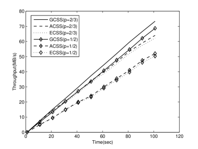
Figure 5: The saturation throughput in the time-varying channel case with different $p$.

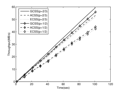
Figure 6: The non-saturation throughput in the time-varying channel case with different $p$.

VII-A2 Time-Varying Channel Case

Fig.5 and Fig.6 show the saturation and non-saturation throughput comparison among GCSS, ACSS and ECSS in the time-varying channel case when $p=2/3$, $1/2$ and $P_{f,th}=0.05$. The comparison indicates that GCSS is able to achieve higher throughput than ACSS and ECSS. This is because GCSS is able to detect and find more spectrum opportunities even when the channel is dynamic. When the number of cooperative SUs becomes larger, our scheme not only finds the available channel quicker but also chooses the channel with maximal rate if more than one available channels are found. Moreover, with the comparison to ECSS, GCSS has the advantage of reducing sensing overhead. As a consequence, the proposed GCSS achieves higher throughput in the time-varying channel case.

In addition, we illustrate the achievable throughput comparison among GCSS, ACSS and ECSS under the complex-valued signal model. Fig.7 and Fig.8 show the saturation and non-saturation throughput comparison among GCSS, ACSS and ECSS in the time-varying channel case, respectively. We observe that GCSS also can obtain higher throughput than that in ACSS and ECSS. This observation indicates the effectiveness of our proposed MAC protocol in both of the real-valued and complex-valued signal model.

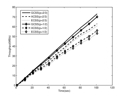
Figure 7: The saturation throughput comparison under complex-valued signal system in the time-varying channel case with different $p$.

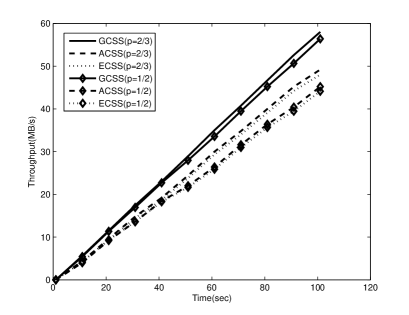
Figure 8: The non-saturation throughput comparison under complex-valued signal system in the time-varying channel case with different $p$.

VII-B Sensing Overhead

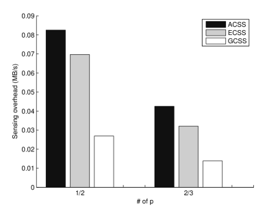
Figure 9: The sensing overhead in the time-invariant channel case with different $p$ for saturation situation.

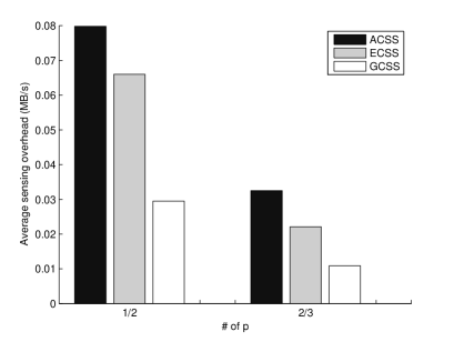
Figure 10: The sensing overhead in the time-invariant channel case with different $p$ for non-saturation situation.

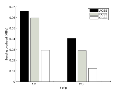
Figure 11: The sensing overhead in the time-varying channel case with different $p$ for saturation situation.

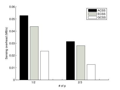
Figure 12: The sensing overhead in the time-varying channel case with different $p$ for non-saturation situation.

VII-B1 Time-Invariant Channel Case

Fig.9 shows sensing overhead among GCSS, ACSS and ECSS in the time-invariant channel case for saturation situation. It is observed that GCSS generates the lowest sensing overhead. This can be explained as follows. GCSS selects the SUs to cooperate by using the SU-selecting algorithm. The algorithm chooses the SUs with low channel available probability ($P_{00}$) for the cooperative sensing. This operation can substantially reduce sensing overhead by avoiding the temporary stopping of the ongoing transmissions when their channels are occupied by PUs. Comparatively, ACSS and ECSS have no similar mechanisms and hence generate higher sensing overhead. Fig.10 shows the sensing overhead for non-saturation situation. Similar observations and conclusions can be made. In addition, we notice that sensing overhead decreases when the channel availability $p$ becomes larger. With more channel availability, there are more chances to find spectrum opportunities in a fixed period; and hence less sensing overheads.

VII-B2 Time-Varying Channel Case

Considering the time-varying channel case, Fig.11 and Fig.12 show the sensing overhead with different channel availability $p$ under saturation and non-saturation situation, respectively. It is clear that sensing overhead becomes lower when the channel availability $p$ increases. Again, the proposed GCSS incurs lower sensing overhead than ACSS and ECSS. With the time-varying channel, we have considered the channel dynamics and rate variation in selecting appropriate SUs to perform sensing. Following this way, sensing overhead in traditional cooperative sensing can be partially avoided.

VIII Conclusion

We design an efficient MAC protocol with selective grouping and cooperative sensing in cognitive radio networks. In our protocol, the cooperative MAC can quickly discover the spectrum opportunities without degrading sensing accuracy. An SU-selecting algorithm is proposed for specifically choosing the cooperative SUs in order to substantially reduce sensing overhead in both time-invariant and time-varying channel cases. We formulate the throughput maximization problems to determine the crucial design parameters and to investigate the trade-off between sensing overhead and throughput. Simulation results show that our proposed protocol can significantly reduced sensing overhead without degrading sensing accuracy.

Yi Liu received his Ph.D. degree from South China University of Technology (SCUT), Guangzhou, China, in 2011. After that, he worked in the Institute of Intelligent Information Processing at Guangdong University of Technology (GDUT). In 2011, he joined the Singapore University of Technology and Design, where he is now a post-doctoral. His research interests include cognitive radio networks, cooperative communications, smart grid and intelligent signal processing.

Shengli Xie [M’01-SM’02] received his M.S. degree in mathematics from Central China Normal University, Wuhan, China, in 1992 and his Ph.D. degree in control theory and applications from South China University of Technology, Guangzhou, China, in 1997. He is presently a Full Professor with the Guangdong University of Technology and a vice head of the Institute of Automation and Radio Engineering. His research interests include automatic control and blind signal processing. He is the author or coauthor of two books and more than 70 scientific papers in journals and conference proceedings. He received the second prize in China’s State Natural Science Award in 2009 for his work on blind source separation and identification.

Rong Yu [S’05, M’08] (yurong@ieee.org) received his Ph.D. from Tsinghua University, Beijing, China, in 2007. After that, he worked in the School of Electronic and Information Engineering of South China University of Technology (SCUT). In 2010, he joined the Institute of Intelligent Information Processing at Guangdong University of Technology (GDUT), where he is now an associate professor. His research interest mainly focuses on wireless communications and networking, including cognitive radio, wireless sensor networks, and home networking. He is the co-inventor of over 10 patents and author or co-author of over 50 international journal and conference papers. Dr. Yu is currently serving as the deputy secretary general of the Internet of Things (IoT) Industry Alliance, Guangdong, China, and the deputy head of the IoT Engineering Center, Guangdong, China. He is the member of home networking standard committee in China, where he leads the standardization work of three standards.

Yan Zhang (yanzhang@ieee.org) received a Ph.D. degree from Nanyang Technological University, Singapore. He is working with Simula Research Laboratory, Norway; and he is an adjunct Associate Professor at the University of Oslo, Norway. He is an associate editor or guest editor of a number of international journals. He serves as organizing committee chairs for many international conferences. His recent research interests include cognitive radio, smart grid, and M2M communications.

Chau Yuen received the B. Eng and PhD degree from Nanyang Technological University, Singapore in 2000 and 2004 respectively. Dr Yuen was a Post Doc Fellow in Lucent Technologies Bell Labs, Murray Hill during 2005. He was a Visiting Assistant Professor of Hong Kong Polytechnic University in 2008. During the period of 2006 - 2010, he worked at the Institute for Infocomm Research (Singapore) as a Senior Research Engineer. He joined Singapore University of Technology and Design as an assistant professor from June 2010. He serves as an Associate Editor for IEEE Transactions on Vehicular Technology. On 2012, he received IEEE Asia-Pacific Outstanding Young Researcher Award.

References

- [1] FCC. “Second memorandum opinion and order. ET Docket No. 10174,” September 2010.
- [2] S. Haykin, “Cognitive radio: brain-empowered wireless communications,” IEEE Journal on Selected Areas in Communications, vol. 23, no. 2, pp. 201-220, February 2005.
- [3] R. Yu. Y. Zhang, S. Gjessing, Y. Chau, S. Xie, and M. Guizani, ”Cognitive Radio based Hierarchical Communications Infrastructure for Smart Grid”, IEEE Network Magazine, vol. 25, no. 5, pp. 6-14, Sept./Oct. 2011.
- [4] T. Wang, L. Song, and Z. Han, Coalitional Graph Games for Popular Content Distribution in Cognitive Radio VANETs, to appear, IEEE Transactions on Vehicular Technologies.
- [5] A. Jovii and P. Viswanath, “Cognitive radio: an information-theoretic perspective,” IEEE Transactions on Information Theory, vol. 55, no. 9, pp. 3945-3958, September 2009.
- [6] F. F. Digham, M. S. Alouini, and M. K. Simon, “On the energy detection of unknown signals over fading channels,” IEEE Transactions on Communications, vol. 55, no. 1, pp. 21-24, January 2007.
- [7] A. Ghasemi and E. S. Sousa, “Spectrum sensing in cognitive radio networks: requirements, challenges and design trade-offs,” IEEE Communication Magzine, vol. 46, no. 4, pp. 32-39, April 2008.
- [8] S. Atapattu, C. Tellambura, and H. Jiang, “Performance of an energy detector over channels with both multipath fading and shadowing,” IEEE Transactions on Wireless Communications, vol. 9, no. 12, pp. 3662-3670, December 2010.
- [9] S. Atapattu, C. Tellambura, and H. Jiang, “Energy detection based cooperative spectrum sensing in cognitive radio networks,” IEEE Transactions on Wireless Communnications, vol. 10, no. 4, pp. 1232-1241, April 2011.
- [10] R.-F Fan and H. Jiang, “Optimal multi-channel cooperative sensing in cognitive radio networks,” IEEE Transactions on Wireless Communications, vol. 9, no. 3, pp. 1128-1138, March 2010.
- [11] J. Shen, S. Liu, L. Zeng, G. Xie, J. Gao and Y. Liu, “Optimisation of cooperative spectrum sensing in cognitive radio network,” IET Communications vol. 3, no. 7, pp.1170-1178, 2009.
- [12] Z. Quan, S. Cui and Sayed A.H, “Optimal multiband joint detection for spectrum sensing in cognitive radio networks,” IEEE Transactions on Signal Processing, vol.57, no. 3, pp. 1128-1140, March, 2009.
- [13] H. Su and X. Zhang, “Cross-layer based opportunistic MAC protocols for QoS provisionings over cognitive radio wireless networks,” IEEE Journal on Selected Areas in Communications, vol. 26, no.1, pp. 118-129, January 2008.
- [14] Y. Liu, R. Yu, and S. Xie, “Optimal cooperative sensing scheme under time-varying channel for cognitive radio networks,” in proc. of IEEE symposium on New Frontiers in Dynamic Spectrum Access Networks (DYSPAN), pp. 352-360, November 2008.
- [15] R. Deng, J. Chen, C. Yuen, P. Cheng, Y. Sun, “Energy-efficient cooperative spectrum sensing by optimal scheduling in sensor-aided cognitive radio networks,” accepted by IEEE Transactions on Vehicular Technology, November 2011.
- [16] S. Xie, Y. Liu, Y. Zhang, and R. Yu “A Parallel Cooperative Spectrum Sensing in Cognitive Radio Networks,” IEEE Transactions on Vehicular Technology, vol. 59, no. 8, pp. 4079-4092, Octorber 2010.
- [17] H. A. Bany Salameh, M. M. Krunz, and O. Younis, “MAC Protocol for Opportunistic Cognitive Radio Networks with Soft Guarantees,” IEEE Transactions on Mobile Computing, vol. 8, no. 10, pp. 1339-1352, October 2009.
- [18] Y.-C Liang, Y. Zeng, E. Peh and A. T. Hoang, “Sensing-throughput tradeoff for cognitive radio networks,” IEEE Transactions on Wireless Communications, vol. 7, no.4, pp. 1326-1337, April 2008.
- [19] H. S. Wang and N. Moayeri, “Finite-state Markov channel-A useful model for radio communication channels,” IEEE Transactions on Vehicular Technology, vol. 44, no. 1, pp. 163-171, February 1995.
- [20] I. Krikidis, N. Devroye, and J. Thompson, “Stability analysis for cognitive radio with multi-access primary transmission,” IEEE Transactions on Wireless Communications, vol. 9, no. 1, pp. 72-77, January 2010.
- [21] Y. -X. Chen, Q. Zhao, and A. Swami, “Distributed Spectrum Sensing and Access in Cognitive Radio Networks With Energy Constraint,” IEEE Transactions on Signal Processing, vol. 57, no. 2, pp. 783-797, February 2009.
- [22] S. R. Singh, B. De Silva, T. Luo, and M. Motani, “Dynamic spectrum cognitive MAC (DySCO-MAC) for wireless mesh & ad hoc networks,” in proc. of INFOCOM IEEE Conference on Computer Communications Workshops, pp. 1-6, March 2010.
- [23] J. Xiang, Y. Zhang and T. Skeie, “Medium Access Control Protocols in Cognitive Radio Networks,” Wiley Wireless Communications and Mobile Computing (WCMC), vol. 10, no. 1, pp. 31-49, 2010.
- [24] M. Timmers, S. Pollin, A. Dejonghe, L. Van der Perre and F. Catthoor, “A distributed multichannel MAC protocol for multihop cognitive radio networks,” IEEE Transactions on Vehicular Technology, vol. 59, no. 1, pp. 446-459, January 2010.
- [25] Q. Chen, Motani. M, W-C. Wong and Nallanathan. A, “Cooperative Spectrum Sensing Strategies for Cognitive Radio Mesh Networks,” IEEE Journal of Selected topics in signal processing, vol. 5, no.1, pp. 110-123, January 2011.
- [26] W. S. Jeon, and D. G. Jeong, “An advanced quiet-period management scheme for cognitive radio systems,” IEEE Transactions on Vehicular Technology, vol. 7, no. 2, pp. 1242-1256, March 2010.
- [27] S. H. Song, K. Hamdi, and K. B. Letaief,“Spectrum sensing with active cognitive systems,” IEEE Transactions on Wireless Communications, vol. 9, no. 6, pp. 1849-1854, June 2010.
- [28] R. Urgaonkar and M. J. Neely, “Opportunistic scheduling with reliablity gurantees in cognitive radio networks,” IEEE Transactions on Mobile Computing, vol. 8, no. 6, pp. 766-777, June 2009.
- [29] L. Kleinrock, “Queuing System,” Wiley, New York, 1975.
- [30] C. Cordeiro, K. Challapali, D. Birru and S. Shankar, “IEEE802.22: The First Worldwide Wireless Standard base on Cognitive Radios,” in proc.of IEEE symposium on New Frontiers in Dynamic Spectrum Access Networks, November 2005.