The standard lateral gene transfer model is statistically consistent for pectinate four-taxon trees

Abstract

Evolutionary events such as incomplete lineage sorting and lateral gene transfer constitute major problems for inferring species trees from gene trees, as they can sometimes lead to gene trees which conflict with the underlying species tree. One particularly simple and efficient way to infer species trees from gene trees under such conditions is to combine three-taxon analyses for several genes using a majority vote approach. For incomplete lineage sorting this method is known to be statistically consistent, however, in the case of lateral gene transfer it is known that a zone of inconsistency does exist for a specific four-taxon tree topology. In this paper we analyze all remaining four-taxon topologies and show that no other inconsistencies exist.

Keywords: Phylogenetic trees, lateral gene transfer, statistical consistency

1 Introduction

A major problem in inferring species trees from gene trees is that different genes often suggest different evolutionary histories [1]. This phenomenon is caused by incomplete lineage sorting and reticulate evolutionary events, i.e. hybridization and lateral gene transfer, and it naturally poses the question, whether the underlying gene tree can be consistently reconstructed from a set of gene trees? In the case of hybridization, it is clear that no single tree can adequately describe the evolution of the taxa under study, and that a network is usually a more appropriate representation. For incomplete lineage sorting recent theoretical work based on the multi-species coalescent has shown that the most probable gene tree topology can differ from the species tree topology, when the number of taxa is greater than three [5]. By contrast it has long been known that for triplets, the matching topology is the most probable topology [8, 3]. Complementary to this, it was recently proved that, under the standard or extended models of lateral gene transfer (LGT), the matching gene tree topology is also the most probable topology for a tree with three taxa; but for the fork-shaped four-taxon tree topology there exist branch lengths for which the matching topology of a triplet has the lowest probability of the three possible topologies [6]. In this paper we start by recalling the two models of lateral gene transfer and the key definitions from [6]. We then give a thorough analysis of the other four-taxon tree topology (the pectinate topology), showing that in this case, the matching topology for a set of three leaves is always the most probable topology, regardless of the location of the fourth taxon. This completes the four-taxon case and implies that four-taxon species trees can be consistently reconstructed using a triplet-based majority vote approach, provided that the branch lengths meet the conditions given in [6].

2 Key definitions

Throughout this paper $X$ will denote a set of $n$ taxa, and $A$ will be a subset of size $3$ of $X$. Let $T$ be a rooted phylogenetic species tree with leaf set $X$ and root $\rho$. Regarding $T$ as a 1-dimensional simplicial complex so each point $p$ in $T$ is either a vertex or an element of an interval that corresponds to an edge, we use a coalescence time scale: $t:T\rightarrow[0,\infty)$ with coalescence time increasing into the past, such that

• $t(p)=0\Leftrightarrow p\text{ is a leaf}$, and

• if $u$ is a descendant of $v$ then $t(u)<t(v)$.

We will denote the time from the present to the most recent common ancestor (MRCA) of the two most closely related taxa in $A$ by $t_{A}$; e.g. if $T|A=a|bc$ then $t_{A}$ is the time from the present to the MRCA of $b$ and $c$.

Linz et al. defines what we will refer to as the standard LGT model in [2]. This model makes the following assumptions:

1. A binary, labeled, rooted and clocklike species tree $T$ is given, as well as all the splitting times along this tree;

2. differences between a specific gene tree and $T$ are only caused by LGT events;

3. the transfer rate is homogeneous per gene and unit time;

4. genes are transfered independently;

5. one copy of the transferred gene still remains in the donor genome; and

6. the transferred gene replaces any existing orthologous counterpart in the acceptor genome.

Based on this model, the authors in [6] considered an extended LGT model, in which the rate of gene transfer between two lineages can be decreasing in the distance between the two lineages. Specifically, letting $d(p,p^{\prime})$ be the evolutionary distance between contemporaneous points $p$ and $p^{\prime}$ in $T$, item three above is replaced by the following assumption:

1. transfer events on $T$ occur as a Poisson process through time, in which the rate of transfer events from point $p$ on a lineage to a contemporaneous point $p^{\prime}$ on another lineage at time $t$ occurs at rate $f(d(p,p^{\prime}),t)$, where $f(d,t)$ is a monotone non-increasing function in $d$ (but can vary non-monotonically in $t$).

2.1 Lateral gene transfer events and transfer sequences

A lateral gene transfer (LGT) on $T$ is an arc from $p\in T$ to $p^{\prime}\in T$ where $t(p)=t(p^{\prime})$ and neither $p$ or $p^{\prime}$ are vertices of $T$. We write $\sigma=(p,p^{\prime})$ to denote this transfer event and we write $t(\sigma)$ for the common value of $t(p)$ and $t(p^{\prime})$. We will assume that no two transfer events occur at exactly the same time.

Let $\underline{\sigma}=\sigma_{1}\ldots\sigma_{k}$ be a sequence of transfer events arranged in increasing $t$-value:

$$0<t(\sigma_{1})<t(\sigma_{2})<\dots<t(\sigma_{k})<t(\rho).$$

Given a species tree $T$ and a transfer sequence $\underline{\sigma}=\sigma_{1}\ldots\sigma_{k}$ on $T$, we obtain an associated gene tree $T[\underline{\sigma}]$. An LGT arc $\sigma$ from point $p$ to $p^{\prime}$ in $T$ describes the event that the gene which was present on the edge at $p^{\prime}$ is replaced by the transfered gene from $p$. Thus, if we trace the history of a gene from the present to the past, each time we encounter an incoming horizontal arc into this edge, we follow this arc (against the direction of the arc). Mathematically this is formalized as follows: For a transfer sequence $\underline{\sigma}=\sigma_{1}\ldots\sigma_{k}$ where $\sigma_{i}=(p_{i},p_{i}^{\prime})$ consider the tree $T$ together with a directed edge for each $\sigma_{i}$ placed between $p_{i}$ and $p_{i}^{\prime}$ for each $i\in\{1,\ldots,k\}$ and regard this network as a one-dimensional simplicial complex. Now for each $i\in\{1,\ldots,k\}$ delete the interval above $p_{i}^{\prime}$ and consider the minimal connected subgraph of the resulting complex that contains $X$. This is $T[\underline{\sigma}]$.

Given the pair $T$, $\underline{\sigma}=\sigma_{1}\ldots\sigma_{k}$, define the following sequence of $X$–trees:

$$T_{0}=T,T_{r}=T_{r-1}[\sigma_{r}].$$

And given $T^{\prime}\in\{T_{0},T_{1},\ldots,T_{k}\}$, a point $p\in T^{\prime}$ and a non-empty subset $Y$ of $X$, let $des_{Y}(T^{\prime},p)$ denote the subset of $Y$ whose elements are descendants of $p$ in $T^{\prime}$.

2.2 Triplet analysis

Let $A$ be a subset of $X$ of size $3$, let $T$ be a phylogenetic species tree on $X$, let $\underline{\sigma}$ be a sequence of transfer events on $T$, and let $\sigma_{r}=(p_{r},p_{r}^{\prime})$ be a specific transfer event on $T$. We say that:

• $\underline{\sigma}$ induces a match for $A$ if $T|A=T[\underline{\sigma}]|A$. Otherwise we say that $\underline{\sigma}$ induces a mismatch for $A$.

• $\sigma_{r}$ is into an $A$-lineage if $des_{A}(T,p_{r}^{\prime})$ is a single element in $A$.

• $\sigma_{r}$ is an $A$-transfer and it transfers $x$ if $des_{A}(T_{r-1},p_{r}^{\prime})=\{x\}$ for some $x\in A$.

• $\sigma_{r}$ is an $A$-moving transfer and it moves $x$ if it transfers $x$ and $des_{A}(T_{r-1},p_{r})=\emptyset$.

• $\sigma_{r}$ is an $A$-joining transfer and it joins $x$ to $y$ if it transfers $x$ and $des_{A}(T_{r-1},p_{r})=\{y\}$ for some $y\in A$.

Note that any $A$–transfer is either an $A$-moving or an $A$-joining transfer.

Let $\underline{\sigma}=\sigma_{1},\sigma_{2},\ldots,\sigma_{k}$ be a sequence of transfer events on $T$ with $t(\sigma_{k})<t_{A}$ and no $A$-joining transfers. Then construct the sequence $T^{\prime}_{0},T^{\prime}_{1},\ldots,T^{\prime}_{k}$ of trees by the following procedure: Set $T^{\prime}_{0}=T$ and construct $T^{\prime}_{i+1}$ from $T^{\prime}_{i}$:

• If $\sigma_{i}$ is not $A$–moving

  1. $T^{\prime}_{i}=T^{\prime}_{i-1}$

• else if $\sigma_{i}=(p_{i},p^{\prime}_{i})$ moves $x\in A$, let $T^{\prime}_{i}$ be the tree obtained from $T_{i-1}^{\prime}$ by

  1. deleting all $p\in T^{\prime}_{i-1}$ with $t(p)<t(\sigma_{i})$,

  2. labeling $p_{i}$ by $x$,

  3. for both $z\in A-\{x\}$, assigning label $z$ to the unique point $p_{z}$ of $T^{\prime}_{i-1}$ that has $t(p_{z})=t(\sigma_{i})$ and $z\in des_{A}(T^{\prime}_{i-1},p_{z})$, and

  4. regarding all other leaves in the tree as unlabeled.

The following two lemmas were given and proved in [6]:

Lemma 1

Let $\underline{\sigma}$ be a sequence of transfer events on a rooted binary $X$–tree $T$ and let $A=\{a,b,c\}\subseteq X$.

1. If $\underline{\sigma}$ induces a mismatch for $A$, then $\underline{\sigma}$ must contain an $A$–transfer with a $t$–value less that $t_{A}$.

2. Moreover precisely one of the following occurs:

   1. $\underline{\sigma}$ has no $A$–transfers. In this case, $\underline{\sigma}$ induces a match for $A$.

   2. $\underline{\sigma}$ contains at least one $A$–joining transfer. In this case, if the first such transfer in $\underline{\sigma}$ joins $x$ to $y$, then $T[\underline{\sigma}]|A=z|xy$ where $\{x,y,x\}=A$.

   3. $\underline{\sigma}$ has no $A$–joining transfers, but it has an $A$–moving transfer with a $t$–value less than $t_{A}$. In this case, if $\sigma_{r}$ denotes the first such $A$–moving transfer in $\underline{\sigma}$ then:

      $$T[\underline{\sigma}]|A=T[\sigma_{r},\ldots,\sigma_{k}]|A.$$

Lemma 2

Suppose $\underline{\sigma}=\sigma_{1},\sigma_{2},\ldots,\sigma_{k}$ is a sequence of transfer events on a rooted binary $X$–tree $T$ with $t(\sigma_{k})<t_{A}$ and with no $A$–joining transfers. Then $T[\underline{\sigma}]|A=T^{\prime}_{k}|A$.

3 Three-taxon trees

For completeness we restate the following result for three-taxon trees from [6]:

Proposition 1

If T has just three taxa, then under the extended LGT model, the probability that a transfer sequence induces a match for the three taxa is strictly greater than the probability it induces either one of the two mismatch topologies (which have equal probability).

4 Four-taxon trees

For four-taxon trees there are two rooted binary tree topologies – the fork-shaped topology with two cherries as shown in Fig. 1(a) and the pectinate tree topology shown in Fig. 1(b). The fork-shaped topology was studied thoroughly in [6], and we will study the pectinate tree topology.

(a) The fork-shaped four-taxon tree topology.

(b) The pectinate four-taxon tree topology $(ab;c;d)$

Figure 1: The two four-taxon tree topologies.

For four-taxon trees $a,b,c,d$, we will write $(ab;c;d)$ to denote the pectinate tree topology depicted in Fig. 1(b). This topology is symmetric to $(ba;c;d)$, $(d;c;ab)$ and $(d;c;ba)$, but no other symmetries hold. For any pectinate four-taxon tree we denote the time of the MRCA of the two most closely related taxa by $t_{2}$, and the time of the MRCA of the three most closely related taxa by $t_{3}$. Thus, for example if the tree has topology $(ab;c;d)$, $t_{2}$ is the time of the MRCA of $a$ and $b$, and $t_{3}$ is the time of the MRCA of $a$, $b$ and $c$.

The main result in this paper is the following theorem:

Theorem 1

Suppose $T$ is a pectinate four-taxon tree and $A=\{a,b,c\}$ is a subset of the leaf set $X$ of $T$, and suppose that $T|A=ab|c$. Let $\underline{\sigma}=\sigma_{1},\sigma_{2},\ldots,\sigma_{k}$ be a random sequence of transfer events on $T$ generated by the standard LGT model of [2], in which the rate of transfer events from point $p$ to a contemporaneous point $p^{\prime}$ is $\lambda$. Then the probability that $\underline{\sigma}$ induces a match on $A$ is strictly higher than the probability that it induces either one of the two mismatch topologies (which have equal probability).

More specifically: Let $\xi_{ab|c}$, $\xi_{ac|b}$ and $\xi_{bc|a}$ denote the disjoint events that $\underline{\sigma}$ induces a tree displaying the triplet topologies $ab|c$, $ac|b$ or $bc|a$, respectively, and let $\mathbb{P}(\xi_{ab|c})$, $\mathbb{P}(\xi_{ac|b})$ and $\mathbb{P}(\xi_{bc|a})$ be the probabilities of these. Then for $\mu=\frac{1}{3}\lambda t_{2}$ and $B=3\lambda(t_{3}-t_{2})$

1. if $T$ is of type $(ab;c;*)$ we have:

   $$\mathbb{P}(\xi_{ab|c})=\frac{1}{3}(1+e^{-7\mu}(\frac{3}{4}e^{-B}e^{-4\mu}+(1-\frac{1}{2}e^{-B})e^{-2\mu}+(1-\frac{1}{4}e^{-B}))),$$ (1)

   and $\mathbb{P}(\xi_{ab|c})>\frac{1}{3}>\mathbb{P}(\xi_{ac|b})=\mathbb{P}(\xi_{bc|a})$ for all values of $t_{2}$ and $t_{3}$;

2. if $T$ is of type $(ab;*;c)$ we have:

   $$\mathbb{P}(\xi_{ab|c})=\frac{1}{3}(1-e^{-7\mu}(\frac{3}{4}e^{-B}e^{-4\mu}-(1-\frac{1}{2}e^{-B})e^{-2\mu}-(1+\frac{5}{4}e^{-B}))),$$ (2)

   and $\mathbb{P}(\xi_{ab|c})>\frac{1}{3}>\mathbb{P}(\xi_{ac|b})=\mathbb{P}(\xi_{bc|a})$ for all values of $t_{2}$ and $t_{3}$; and

3. if $T$ is of type $(a*;b;c)$ or $(b*;a;c)$ we have:

   $$\mathbb{P}(\xi_{ab|c})=\frac{1}{3}(1+e^{-7\mu}(\frac{3}{8}e^{-B}e^{-4\mu}-(\frac{1}{2}-\frac{1}{4}e^{-B})e^{-2\mu}+(\frac{1}{2}+\frac{11}{8}e^{-B}))),$$ (3)

   and $\mathbb{P}(\xi_{ab|c})>\frac{1}{3}>\mathbb{P}(\xi_{ac|b})=\mathbb{P}(\xi_{bc|a})$ for all values of $t_{2}$ and $t_{3}$.

The proof of Theorem 1 relies on the analysis of the discrete $7$-state Markov chain whose transition digraph is illustrated in Fig. 2. We will therefore study this Markov chain thoroughly, before we dive into the proof of the theorem.

4.1 The 7-state continuous-time Markov chain

Let $Z_{t}:t\geq 0$ be the $7$–state continuous-time Markov chain defined by the rate matrix

$$Q=\left[\begin{array}[]{ccccccc}-3&2&0&0&0&0&1\\ 1&-2&1&0&0&0&0\\ 0&1&-3&1&1&0&0\\ 0&0&1&-2&1&0&0\\ 0&0&1&1&-3&1&0\\ 0&0&0&0&1&-2&1\\ 1&0&0&0&0&2&-3\\ \end{array}\right]$$

and illustrated in Fig. 2, let $p_{r}(t)=\mathbb{P}(Z_{t}=r)$, and let $\mathbf{p}(t)=[p_{0}(t),\ldots,p_{6}(t)]$. Then by standard Markov chain theory [7]

$$\frac{d}{dt}\mathbf{p(t)}=\mathbf{p(t)}Q\quad\text{ and }\quad\mathbf{p}(t)=\mathbf{p}(0)\exp(Qt).$$

Figure 2: The 7 state continuous-time Markov model.

The Markov chain is easily seen to be irreducible and ergodic and thus it has a stationary distribution $\boldsymbol{\pi}$. To find $\boldsymbol{\pi}$ let

$$P=\left[\begin{array}[]{ccccccc}0&\frac{2}{3}&0&0&0&0&\frac{1}{3}\\ \frac{1}{2}&0&\frac{1}{2}&0&0&0&0\\ 0&\frac{1}{3}&0&\frac{1}{3}&\frac{1}{3}&0&0\\ 0&0&\frac{1}{2}&0&\frac{1}{2}&0&0\\ 0&0&\frac{1}{3}&\frac{1}{3}&0&\frac{1}{3}&0\\ 0&0&0&0&\frac{1}{2}&0&\frac{1}{3}\\ \frac{1}{3}&0&0&0&0&\frac{2}{3}&0\\ \end{array}\right]$$

be the transition probability matrix of $Q$ defined by

$$p_{ij}=\left\{\begin{array}[]{cl}\frac{q_{ij}}{\sum_{k\neq i}q_{ik}}&\mbox{ if $i\neq j$}\\ 0&\mbox{ otherwise}\end{array}\right.$$

Then $\boldsymbol{\pi}$ can be computed as

$$\boldsymbol{\pi}=\frac{-\boldsymbol{\phi}~{}D_{Q}^{-1}}{||\boldsymbol{\phi}D_{Q}^{-1}||_{1}},$$

where $\boldsymbol{\phi}$ is the unique solution summing to $1$ of $\boldsymbol{\phi}(I-P)=\mathbf{0}$ and $D_{Q}$ is the $7\times 7$ diagonal matrix having the same diagonal as $Q$ [7]. Using this we find

$$\boldsymbol{\pi}=\left(\frac{1}{12},\frac{2}{12},\frac{2}{12},\frac{2}{12},\frac{2}{12},\frac{2}{12},\frac{1}{12}\right).$$

The eigenvalues of $Q$ are

$$\lambda_{1}=-5,\quad\lambda_{2} =-4,\quad\lambda_{3}=-4$$

$$\lambda_{4}=-3,\quad\lambda_{5} =-1,\quad\lambda_{6}=-1$$

$$\lambda_{7} =0$$

with corresponding eigenvectors:

$$\mathbf{v_{1}} =(-2,1,-1,0,1,-1,2)$$

$$\mathbf{v_{2}} =(-1,0,1,0,-1,0,1)$$

$$\mathbf{v_{3}} =(-2,1,0,1,-2,1,0)$$

$$\mathbf{v_{4}} =(2,-1,-1,2,-1,-1,2)$$

$$\mathbf{v_{5}} =(4,3,-1,-3,-2,0,2)$$

$$\mathbf{v_{6}} =(-2,-2,0,1,1,1,0)$$

$$\mathbf{v_{7}} =(1,1,1,1,1,1,1)$$

Thus every element $p_{r}(t)$ for $r=0,1,\ldots,6$ and $t\geq 0$ is of the form:

$$p_{r}(t)=a_{r}+b_{r}\exp(-t)+c_{r}\exp(-3t)+d_{r}\exp(-4t)+e_{r}\exp(-5t)$$

for constants $a_{j},\dots,d_{j}$ depending on $\mathbf{p}(0)$. To find these constants we will solve the set of linear equations given by

$$\mathbf{p}(t)=\left[e^{-5t},e^{-4t},e^{-4t},e^{-3t},e^{-1t},e^{-1t},1\right]X,$$

where $X$ is a $7\times 7$ matrix containing the constants. Let $D$ be the $7\times 7$ diagonal matrix with the eigenvalues of $Q$, $\lambda_{1},\lambda_{2},\ldots,\lambda_{7}$, being the diagonal entries, and let $V$ be the $7\times 7$ matrix with the eigenvector $\mathbf{v_{i}}$ corresponding to $\lambda_{i}$ being column $i$ of $V$. Then $Q=VDV^{-}1$, and we get

$$\mathbf{p}(t) =\mathbf{p}(0)\exp(Qt)$$

$$=\mathbf{p}(0)\exp(VDV^{-1}t)$$

$$=\mathbf{p}(0)V\exp(Dt)V^{-1}$$

$$=\mathbf{p}(0)V\left[\begin{array}[]{ccccccc}e^{-5t}&&&&&&\\ &e^{-4t}&&&\makebox(0.0,0.0)[]{\text{\huge 0}}&&\\ &&e^{-4t}&&&&\\ &&&e^{-3t}&&&\\ &&&&e^{-t}&&\\ &\makebox(0.0,0.0)[]{\text{\huge 0}}&&&&e^{-t}&\\ &&&&&&1\end{array}\right]V^{-1}.$$

Thus the set of linear equations we need to solve reduces to

$$\left[\begin{array}[]{c}e^{-5t}\\ e^{-4t}\\ e^{-4t}\\ e^{-3t}\\ e^{-1t}\\ e^{-1t}\\ 1\end{array}\right]^{T}X=\mathbf{p}(0)V\left[\begin{array}[]{ccccccc}e^{-5t}&&&&&&\\ &e^{-4t}&&&\makebox(0.0,0.0)[]{\text{\huge 0}}&&\\ &&e^{-4t}&&&&\\ &&&e^{-3t}&&&\\ &&&&e^{-1t}&&\\ &\makebox(0.0,0.0)[]{\text{\huge 0}}&&&&e^{-1t}&\\ &&&&&&1\end{array}\right]V^{-1}.$$

Doing this with $\mathbf{p}(0)=(1,0,0,0,0,0,0)$, we get

$$\mathbf{p}(t)=\frac{1}{12}\left[\begin{array}[]{c}e^{-5t}\\ e^{-4t}\\ e^{-4t}\\ e^{-3t}\\ e^{-1t}\\ e^{-1t}\\ 1\end{array}\right]^{T}\left[\begin{array}[]{ccccccc}3&-3&3&0&-3&3&-3\\ 1&2&-6&2&2&2&-3\\ 2&-4&4&-4&4&-4&2\\ 2&-2&-2&4&-2&-2&2\\ 2&-2&-6&-8&-2&10&6\\ 1&7&5&4&-1&-11&-5\\ 1&2&2&2&2&2&1\end{array}\right].$$ (4)

From this representation of $\mathbf{p}(t)$ we immediately get the following Lemma, which will be usefull in the process of proving Theorem 1.

Lemma 3

For all $t>0$ and $\mathbf{p}(0)=(1,0,0,0,0,0,0)$

$$p_{1}(t)=-\frac{1}{4}e^{-5t}-\frac{1}{6}e^{-4t}-\frac{1}{6}e^{-3t}+\frac{5}{12}e^{-t}+\frac{1}{6},$$

$$p_{5}(t)=\frac{1}{4}e^{-5t}-\frac{1}{6}e^{-4t}-\frac{1}{6}e^{-3t}-\frac{1}{12}e^{-t}+\frac{1}{6},$$

$$p_{0}(t)+p_{6}(t)=\frac{1}{6}e^{-4t}+\frac{1}{3}e^{-3t}+\frac{1}{3}e^{-t}+\frac{1}{6}\text{, and}$$

$$p_{1}(t)+p_{3}(t)+p_{5}(t)=\frac{1}{2}-\frac{1}{2}e^{-4t}.$$

Similarly if $\mathbf{p}(0)=(0,0,0,0,0,1,0)$ we get

$$\mathbf{p}(t)=\frac{1}{24}\left[\begin{array}[]{c}e^{-5t}\\ e^{-4t}\\ e^{-4t}\\ e^{-3t}\\ e^{-1t}\\ e^{-1t}\\ 1\end{array}\right]^{T}\left[\begin{array}[]{ccccccc}3&-3&3&0&-3&3&-3\\ 0&0&0&0&0&0&0\\ -2&4&-4&4&-4&4&-2\\ -2&2&2&-4&2&2&-2\\ 0&0&0&0&0&0&0\\ -1&-7&-5&-4&1&11&5\\ 2&4&4&4&4&4&2\end{array}\right],$$ (5)

and the following Lemma follows immediately:

Lemma 4

For all $t>0$ and $\mathbf{p}(0)=(0,0,0,0,0,1,0)$

$$p_{5}(t)=\frac{1}{8}e^{-5t}+\frac{1}{6}e^{-4t}+\frac{1}{12}e^{-3t}+\frac{11}{24}e^{-t}+\frac{1}{6},$$

$$p_{0}(t)+p_{6}(t)=-\frac{1}{6}e^{-4t}-\frac{1}{6}e^{-3t}+\frac{1}{6}e^{-t}+\frac{1}{6}\text{, and}$$

$$p_{1}(t)+p_{3}(t)+p_{5}(t)=\frac{1}{2}e^{-4t}+\frac{1}{2}.$$

4.2 Proof of part (i)

Let $T$ be a four-taxon tree over the set of taxa $X=\{a,b,c,*\}$ with topology $(ab;c;*)$ (here $*$ refers to the fourth taxon, the identity of which plays no role when we come to consider the topology of the triple $a,b,c$), let $A=\{a,b,c\}$, and let $\underline{\sigma}=\sigma_{1},\sigma_{2},\ldots,\sigma_{k}$ be a random sequence of transfer events on $T$ generated by the standard LGT model in which the rate of transfer events from point $p$ to point $p^{\prime}$ is $\lambda$. Let $\xi$ be any one of the three events $\xi_{ab|c}$, $\xi_{ac|b}$ or $\xi_{bc|a}$, and let $J$ denote the (stochastic) number of $A$–joining transfers between time $t=0$ and time $t=t_{2}$. Then by the law of total probability

$$\mathbb{P}(\xi) =\mathbb{P}(\xi,J>0)+\mathbb{P}(\xi,J=0)$$ (6)

$$=\mathbb{P}(\xi|J>0)\mathbb{P}(J>0)+\mathbb{P}(\xi|J=0)\mathbb{P}(J=0).$$

To find $\mathbb{P}(J>0)$ and $\mathbb{P}(J=0)$ we observe that $J$ has a Poisson distribution with mean $2\lambda t_{2}$, since at any moment in the interval $[0,t_{2}]$, there are four lineages, three of which lead to leaves in $A$, and for each of these, the rate of transfer from that $A$–lineage to another $A$–lineage is $\lambda\cdot 2/3$. This means that the cumulative rate of an $A$–joining transfer is $3\cdot\lambda\cdot 2/3=2\lambda$ at any given time in the interval $[0,t_{2}]$. Thus

$$\mathbb{P}(J=0)=e^{-2\lambda t_{2}}\quad\text{and}\quad\mathbb{P}(J>0)=1-e^{-2\lambda t_{2}},$$

and we arrive at

$$\mathbb{P}(\xi)=\mathbb{P}(\xi|J>0)(1-e^{-2\lambda t_{2}})+\mathbb{P}(\xi|J=0)e^{-2\lambda t_{2}},$$ (7)

where $\xi$ is any one of the events $\xi_{ab|c}$, $\xi_{ac|b}$ or $\xi_{bc|a}$. We will now consider the two factors $\mathbb{P}(\xi|J>0)$ and $\mathbb{P}(\xi|J=0)$ in turn.

$\boldsymbol{\mathbb{P}(\xi|J>0)}$: Lemma 1.2b tells us that if there is at least one $A$–joining transfer in $\underline{\sigma}$, then the first one of these decides the resulting topology of $T[\underline{\sigma}]|A$. There are $6$ possibilities for this first $A$–joining transfer: $a\rightarrow b$, $a\leftarrow b$, $a\rightarrow c$, $a\leftarrow c$, $b\rightarrow c$ and $b\leftarrow c$. The first two of these will give $T[\underline{\sigma}]|A=ab|c$, the next two will give $T[\underline{\sigma}]|A=ac|b$, while the last two will give $T[\underline{\sigma}]|A=bc|a$. As they are all equally likely, we get

$$\mathbb{P}(\xi|J>0)=\frac{1}{3}.$$ (8)

$\boldsymbol{\mathbb{P}(\xi|J=0)}$: When $J=0$, Lemma 1.2c tells us that we need to look at the $A$–moving transfers, and Lemma 2 tells us that $T^{\prime}_{k}$, as described in the preamble of the two lemmas, will induce the same topology on $A$ as $T$. The process of $A$–moving transfers between time $t=0$ and $t=t_{2}$ is a Poisson process in which the rate at which any given $x\in A$ is moved is $\frac{1}{3}\lambda$, since each of the three $A$–lineages can be moved to only one ($*$) out of three other lineages (otherwise it would be an $A$–joining transfer). Note that this process is independent of $J$ as the source point of an $A$–joining transfer will always have an element of $A$ as a descendant, whereas the source point of an $A$–moving transfer will not. The walk in tree space, corresponding to moving along the sequence $T^{\prime}_{0},T^{\prime}_{1},\ldots,T^{\prime}_{k}$, as this process proceeds is described by the Markov chain illustrated in Fig. 3 with rate $\frac{1}{3}\lambda$ of moving from any state to each of its neighbors.

Figure 3: The 12-cycle describing the walk in tree space corresponding to moving along the sequence $T^{\prime}_{0},T^{\prime}_{1},\ldots,T^{\prime}_{k}$.

Now let $Z_{t}:t\geq 0$ be a continuous-time symmetric random walk on the $12$-cycle illustrated in Fig. 3, where the instantaneous rate of moving from one node to one of its neighbors is $\frac{1}{3}\lambda$. As $T$ has topology $(ab;c;*)$ the random walk’s initial state is state $1$. The 7-state model, treated in the previous section, is obtained from the model in Fig. 3 by grouping state $2$ and $12$, $3$ and $11$, $4$ and $10$, $5$ and $9$, and $6$ and $8$. So, accordingly, let $p_{r}(t)$ for $r=0,1,\ldots,6$ be the probability that, after running this process for time $t$, $Z_{t}$ is at a state that can be reached in $r$ steps from state $1$, taking no diagonal edges, and let $\mathbf{p}(t)=(p_{0}(t),p_{1}(t),p_{2}(t),p_{3}(t),p_{4}(t),p_{5}(t),p_{6}(t))$. Then $\mathbf{p}(0)=(1,0,0,0,0,0,0)$ and $\mathbf{p}(t)$ behaves as described in Lemma 3 after rescaling time by a factor $\frac{1}{3}\lambda$.

Let $\tau_{i}$ be the state of the random walk on the 12-cycle at time $t_{2}$. Lemma 2 then ensures, that if $\underline{\sigma}^{\prime}$ is the sequence of $A$-moving transfers between $t=0$ and $t=t_{2}$, then $T[\underline{\sigma}^{\prime}]$ resolves $a,b$ and $c$ in the same way as $\tau_{i}$ does. At time $t=t_{2}$ the random walk on the $12$-cycle is in one of the following states:

• $1$ in which case $T[\sigma]|A=ab|c$ with probability $1$ regardless of any LGT events after $t_{2}$.

• $2$ or $12$ in which case

  • $T[\sigma]|A=ab|c$ with probability $\frac{1}{3}$ if there is at least one transfer event between $t_{2}$ and $t_{3}$, and

  • $T[\sigma]|A=ac|b$ and $T[\sigma]|A=bc|a$ both have probability

    • $\frac{1}{2}$ if there is no LGT events between $t_{2}$ and $t_{3}$, and

    • $\frac{1}{3}$ if there is at least one transfer between $t_{2}$ and $t_{3}$.

• $3$ or $11$ in which case $T[\sigma]|A=ac|b$ and $T[\sigma]|A=bc|a$ both have probability $\frac{1}{2}$ regardless of any LGT events after $t_{2}$.

• $4$ or $10$ in which case

  • $T[\sigma]|A=ab|c$ with probability $\frac{1}{3}$ if there is at least one transfer event between $t_{2}$ and $t_{3}$, and

  • $T[\sigma]|A=ac|b$ and $T[\sigma]|A=bc|a$ both have probability

    • $\frac{1}{2}$ if there is no LGT events between $t_{2}$ and $t_{3}$, and

    • $\frac{1}{3}$ if there is at least one transfer between $t_{2}$ and $t_{3}$.

• $5$ or $9$ in which case $T[\sigma]|A=ac|b$ and $T[\sigma]|A=bc|a$ both have probability $\frac{1}{2}$ regardless of any LGT events after $t_{2}$.

• $6$ or $8$ in which case

  • $T[\sigma]|A=ab|c$ with probability

    • $1$ if there is no LGT events between $t_{2}$ and $t_{3}$, or

    • $\frac{1}{3}$ if there is at least one transfer event between $t_{2}$ and $t_{3}$, and

  • $T[\sigma]|A=ac|b$ and $T[\sigma]|A=bc|a$ both have probability $\frac{1}{3}$ if there is at least one transfer between $t_{2}$ and $t_{3}$.

• $7$ in which case $T[\sigma]|A=ab|c$ with probability $1$ regardless of any LGT events after $t_{2}$.

Let $\mu=\frac{1}{3}\lambda t_{2}$ and $B=3\lambda(t_{3}-t_{2})$. Then the probability that there is no LGT event between $t_{2}$ and $t_{3}$ is $e^{-B}$, and the probability that there is at least one LGT event in the same time span is thus $1-e^{-B}$. Consequently we get the following from combining the cases above:

$$\mathbb{P}(\xi_{ab|c}|J=0) =p_{0}(\mu)\cdot 1$$ (9)

$$+p_{1}(\mu)\cdot\frac{1}{3}(1-e^{-B})$$

$$+p_{2}(\mu)\cdot 0$$

$$+p_{3}(\mu)\cdot\frac{1}{3}(1-e^{-B})$$

$$+p_{4}(\mu)\cdot 0$$

$$+p_{5}(\mu)\cdot(1\cdot e^{-B}+\frac{1}{3}(1-e^{-B}))$$

$$+p_{6}(\mu)\cdot 1$$

$$=p_{0}(\mu)+p_{6}(\mu)+p_{5}(\mu)e^{-B}+\frac{1}{3}(1-e^{-B})(p_{1}(\mu)+p_{3}(\mu)+p_{5}(\mu))$$

Similarly we get

$$\mathbb{P}(\xi_{ac|b}|J=0)=\mathbb{P}(\xi_{bc|a}|J=0) =\frac{1}{2}(p_{2}(\mu)+p_{4}(\mu))+\frac{1}{2}e^{-B}(p_{1}(\mu)+p_{3}(\mu))$$ (10)

$$+\frac{1}{3}(1-e^{-B})(p_{1}(\mu)+p_{3}(\mu)+p_{5}(\mu)).$$

Now using Lemma 3, we get

$$\mathbb{P}(\xi_{ab|c}|J=0) =\frac{1}{6}e^{-4\mu}+\frac{1}{3}e^{-3\mu}+\frac{1}{3}e^{-\mu}+\frac{1}{6}$$ (11)

$$+(\frac{1}{4}e^{-5\mu}-\frac{1}{6}e^{-4\mu}-\frac{1}{6}e^{-3\mu}-\frac{1}{12}e^{-\mu}+\frac{1}{6})e^{-B}$$

$$+(\frac{1}{2}-\frac{1}{2}e^{-4\mu})\frac{1}{3}(1-e^{-B})$$

$$=\frac{1}{3}(1+\frac{3}{4}e^{-5\mu}e^{-B}+(1-\frac{1}{2}e^{-B})e^{-3\mu}+(1-\frac{1}{4}e^{-B})e^{-\mu}),$$

and finally, using (7) and (8), we arrive at

$$\mathbb{P}(\xi_{ab|c}) =\frac{1}{3}(1+e^{-7\mu}(\frac{3}{4}e^{-B}e^{-4\mu}+(1-\frac{1}{2}e^{-B})e^{-2\mu}+(1-\frac{1}{4}e^{-B}))).$$ (12)

From this it is easy to see that $\mathbb{P}(\xi)>\frac{1}{3}$ for all positive values of $\mu$ and $B$, as $\frac{3}{4}e^{-B}e^{-4\mu}>0$, $(1-\frac{1}{2}e^{-B})e^{-2\mu}>0$ and $1-\frac{1}{4}e^{-B}>0$. Hence since $\mathbb{P}(\xi_{ac|b})=\mathbb{P}(\xi_{bc|a})$ we get $\mathbb{P}(\xi_{ab|c})>\frac{1}{3}>\mathbb{P}(\xi_{ac|b})=\mathbb{P}(\xi_{bc|a})$.

A plot of $\mathbb{P}(\xi_{ab|c})$ as a function of $\mu$ and $B$ is shown in Fig. 4.

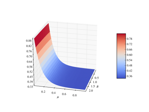
Figure 4: $\mathbb{P}(\xi_{ab|c})$ for four-taxon trees with the $(ab;c;*)$ topology as a function of $B=3\lambda(t_{3}-t_{2})$ and $\mu=\frac{1}{3}\lambda t_{2}$.

4.3 Proof of part (ii)

The proof of the claim in part (ii) of Theorem 1 is completely analogous to the proof of part (i) up until the formulation of $\mathbb{P}(\xi_{a|bc})$ in (9). When the original tree $T$ has topology $(ab;*;c)$, the random walk starts in state $7$ (not state $1$ as it did before). Because of the symmetries of the two Markov models, this means that $p_{0}(\mu)$ and $p_{6}(\mu)$ swap places in (9), $p_{1}(\mu)$ and $p_{5}(\mu)$ swap places, and $p_{2}(\mu)$ and $p_{4}(\mu)$ swap places. Consequently we get

$$\mathbb{P}(\xi_{ab|c}|J=0)=p_{0}(\mu)+p_{6}(\mu)+p_{1}(\mu)e^{-B}+\frac{1}{3}(1-e^{-B})(p_{1}(\mu)+p_{3}(\mu)+p_{5}(\mu))$$

and $\mathbb{P}(\xi_{ac|b})=\mathbb{P}(\xi_{bc|a})$. Now using Lemma 3 we get

$$\mathbb{P}(\xi_{ab|c}|J=0)=\frac{1}{3}(1-\frac{3}{4}e^{-5\mu}e^{-B}+(1-\frac{1}{2}e^{-B})e^{-3\mu}+(1+\frac{5}{4}e^{-B})).$$

And using (7) and (8) we arrive at

$$\mathbb{P}(\xi_{ab|c})=\frac{1}{3}(1-e^{-7\mu}(\frac{3}{4}e^{-4\mu}e^{-B}-(1-\frac{1}{2}e^{-B})e^{-2\mu}-(1+\frac{5}{4}e^{-B}))).$$

We will now show that $\mathbb{P}(\xi_{ab|c})>\frac{1}{3}$ for all $\mu,B>0$. From the above we observe that $\mathbb{P}(\xi_{ab|c})>\frac{1}{3}$ if and only if

$$0>\frac{3}{4}e^{-4\mu}e^{-B}-(1-\frac{1}{2}e^{-B})e^{-2\mu}-(1+\frac{5}{4}e^{-B})$$ (13)

$$\Updownarrow$$

$$e^{-2\mu}+1>e^{-B}(\frac{3}{4}e^{-4\mu}+\frac{1}{2}e^{-2\mu}-\frac{5}{4}).$$

Now note that

$$\begin{array}[]{llll}\frac{3}{4}e^{-4\mu}+\frac{1}{2}e^{-2\mu}-\frac{5}{4}&\rightarrow&0&\text{ for }\quad\mu\rightarrow 0\text{, and}\\ &&\\ \frac{3}{4}e^{-4\mu}+\frac{1}{2}e^{-2\mu}-\frac{5}{4}&\rightarrow&-\frac{5}{4}&\text{ for }\quad\mu\rightarrow\infty.\\ \end{array}$$

Thus $\frac{3}{4}e^{-4\mu}+\frac{1}{2}e^{-2\mu}-\frac{5}{4}<0$ for all $\mu>0$. This means that (13) is true for all $\mu,B>0$ since the left-hand side is always positive and the right-hand side is always negative. We conclude that $\mathbb{P}(\xi_{ab|c})>\frac{1}{3}$ for all $\mu,B>0$ and hence for all values of $t_{2}$ and $t_{3}$.

A plot of $\mathbb{P}(\xi_{ab|c})$ as a function of $\mu$ and $B$ is shown in Fig. 5.

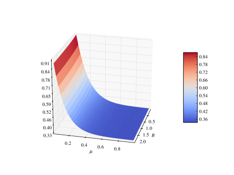
Figure 5: $\mathbb{P}(\xi_{ab|c})$ for four-taxon trees with the $(ab;*;c)$ topology as a function of $B=3\lambda(t_{3}-t_{2})$ and $\mu=\frac{1}{3}\lambda t_{2}$.

4.4 Proof of part (iii)

The proof of part (iii) of Theorem 1 is completely analogous to the proof of part (i) and (ii) given in Section 4.2 and 4.2 up until the computation of $\mathbb{P}(\xi|J=0)$.

As in the previous two sections let $Z_{t}:t\geq 0$ be a continuous-time symmetric random walk on the 12-cycle illustrated in Fig. 3, where the instantaneous rate of moving from one node to one of its neighbors is $\frac{1}{3}\lambda$. But this time, as $T$ has topology $(a*;b;c)$ or $(b*;a;c)$, the random walk starts in either state $6$ or $8$. Let $p_{0}(t),p_{1}(t),\ldots,p_{6}(t)$ be defined as in Section 4.2 by

$$p_{0}(t) =\mathbb{P}(Z_{t}=1)$$

$$p_{1}(t) =\mathbb{P}(Z_{t}=2\text{ or }Z_{t}=12)$$

$$p_{2}(t) =\mathbb{P}(Z_{t}=3\text{ or }Z_{t}=11)$$

$$p_{3}(t) =\mathbb{P}(Z_{t}=4\text{ or }Z_{t}=10)$$

$$p_{4}(t) =\mathbb{P}(Z_{t}=5\text{ or }Z_{t}=9)$$

$$p_{5}(t) =\mathbb{P}(Z_{t}=6\text{ or }Z_{t}=8)$$

$$p_{6}(t) =\mathbb{P}(Z_{t}=7),$$

and let $\mathbf{p}(t)=(p_{0}(t),p_{1}(t),p_{2}(t),p_{3}(t),p_{4}(t),p_{5}(t),p_{6}(t))$. Then $\mathbf{p}(0)=(0,0,0,0,0,1,0)$ and $\mathbf{p}(t)$ behaves as described in Lemma 4 after rescaling time by a factor $\frac{1}{3}\lambda$. As in Section 4.2 we get

$$\mathbb{P}(\xi_{ab|c}|J=0)=p_{0}(\mu)+p_{6}(\mu)+\frac{1}{3}(1-e^{-B})(p_{1}(\mu)+p_{3}(\mu)+p_{5}(\mu))\ e^{-B}p_{5}(\mu)$$

and $\mathbb{P}(\xi_{ac|b}=\mathbb{P}(\xi_{bc|a})$. Using Lemma 4 we now get

$$\mathbb{P}(\xi_{ab|c}|J=0)=\frac{1}{3}(1+\frac{3}{8}e^{-B}e^{-5\mu}-(\frac{1}{2}-\frac{1}{4}e^{-B})e^{-3\mu}+(\frac{1}{2}+\frac{11}{8}e^{-B})e^{-\mu}),$$

and we finally arrive at

$$\mathbb{P}(\xi_{ab|c})=\frac{1}{3}(1+e^{-7\mu}(\frac{3}{8}e^{-B}e^{-4\mu}-(\frac{1}{2}-\frac{1}{4}e^{-B})e^{-2\mu}+(\frac{1}{2}+\frac{11}{8}e^{-B}))).$$

To show that $\mathbb{P}(\xi_{ab|c})>\frac{1}{3}$ for all $\mu,B>0$ we observe that $\mathbb{P}(\xi_{ab|c})>\frac{1}{3}$ if and only if

$$0<\frac{3}{8}e^{-B}e^{-5\mu}-(\frac{1}{2}-\frac{1}{4}e^{-B})e^{-3\mu}+(\frac{1}{2}+\frac{11}{8}e^{-B})e^{-\mu}$$ (14)

$$\Updownarrow$$

$$\frac{1}{2}(e^{-2\mu}-1)<e^{-B}(\frac{3}{8}e^{-4\mu}+\frac{1}{4}e^{-2\mu}+\frac{11}{8}).$$

Note that

$$\begin{array}[]{llll}\frac{3}{8}e^{-4\mu}+\frac{1}{4}e^{-2\mu}+\frac{11}{8}&\rightarrow&2&\text{ for }\quad\mu\rightarrow 0\text{, and}\\ &&&\\ \frac{3}{8}e^{-4\mu}+\frac{1}{4}e^{-2\mu}+\frac{11}{8}&\rightarrow&\frac{11}{8}&\text{ for }\quad\mu\rightarrow\infty.\\ \end{array}$$

Thus $\frac{3}{8}e^{-4\mu}+\frac{1}{4}e^{-2\mu}+\frac{11}{8}>0$ for all $\mu>0$. This means that (14) is true for all $\mu,B>0$, as the left-hand side is always negative, and the right-hand side is always positive. We therefore conclude that $\mathbb{P}(\xi_{ab|c})>\frac{1}{3}>\mathbb{P}(\xi_{ac|b})=\mathbb{P}(\xi_{bc|a})$ for all values of $t_{2}$ and $t_{3}$.

A plot of $\mathbb{P}(\xi_{ab|c})$ as a function of $\mu$ and $B$ is shown in Fig. 6.

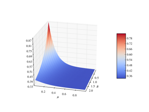
Figure 6: $\mathbb{P}(\xi_{ab|c})$ for four-taxon trees with the either the $(a*;b;c)$ or the $(b*;a;c)$ topology as a function of $B=3\lambda(t_{3}-t_{2})$ and $\mu=\frac{1}{3}\lambda t_{2}$.

5 Limits

It is interesting and reaffirming to study the limits of the probabilities stated in Theorem 1 when $t_{2}$, $t_{3}$ or $t_{3}-t_{2}$ approaches $0$. When $t_{3}$ approaches $0$ we leave no time for any transfer events to occur before the first three taxa have coalesced. We therefore expect to see that the triplet topology from the species tree is preserved. And indeed $\mathbb{P}(\xi_{ab|c})\rightarrow 1$ and $\mathbb{P}(\xi_{ac|b})=\mathbb{P}(\xi_{bc|a})\rightarrow 0$ as $t_{3}\rightarrow 0$ in all three cases of Theorem 1 (topology $(ab;c;*)$, $(ab;*;c)$ and $(a*;b;c)$ or $(b*;a;c)$).

When $t_{2}$ approaches $0$ we leave no time for any transfer events, splitting up the two most closely related taxa, to occur, since such events would have to happen before time $t_{2}$. Thus we expect that the grouping of these two is preserved from the species tree topology. We can recognize this behaviour in the limits for the topologies $(ab;c;*)$ and $(ab;*;c)$, where $\mathbb{P}(\xi_{ab|c})\rightarrow 1$ and $\mathbb{P}(\xi_{ac|b})=\mathbb{P}(\xi_{bc|a})\rightarrow 0$ as $t_{2}$ approaches $0$. Taxa $a$ and $b$ are here invariably grouped together, and the matching topology is preserved regardless of any transfer events after time $t_{2}$. If the species tree has topology $(a*;b;c)$ or $(b*;a;c)$ then the species tree’s triplet topology is preserved with probability $1$ if no transfer events occur between $t_{2}$ and $t_{3}$ and with probability $\frac{1}{3}$ if at least one transfer event occurs between $t_{2}$ and $t_{3}$ (such an event would be an $A$-joining event). Similarly a mismatching topology can only be obtained if at least one transfer event occurs between $t_{2}$ and $t_{3}$, in which case either of the two topologies is obtained with probability $\frac{1}{3}$. Indeed we see from Theorem 1 that $\mathbb{P}(\xi_{ab|c})\rightarrow e^{-B}+\frac{1}{3}(1-e^{-B})$ and $\mathbb{P}(\xi_{ac|b})=\mathbb{P}(\xi_{bc|a})\rightarrow\frac{1}{3}(1-e^{-B})$ as $t_{2}$ approaches $0$.

When $t_{3}-t_{2}$ approaches $0$ the triplet topology in a gene tree entirely depends on the transfer events taking place before time $t_{2}$. But since any kind of events can happen in this period of time, this case is more complex than the two previous cases. The limits obtained from the probabilities in Theorem 1 are as follows:

• If $T$ has topology $(ab;c;*)$ then

  $$\mathbb{P}(\xi_{ab|c})\rightarrow\frac{1}{3}(1+e^{-7\mu}(\frac{3}{4}+\frac{3}{4}e^{-4\mu}+\frac{1}{2}e^{-2\mu}))>\frac{1}{3}\;\forall\mu>0\text{, and}$$

  $$\mathbb{P}(\xi_{ac|b})=\mathbb{P}(\xi_{bc|a})\rightarrow\frac{1}{3}(1-\frac{e^{-7\mu}}{2}(\frac{3}{4}+\frac{3}{4}e^{-4\mu}+\frac{1}{2}e^{-2\mu}))<\frac{1}{3}\;\forall\mu>0.$$

• If $T$ has topology $(ab;*;c)$ then

  $$\mathbb{P}(\xi_{ab|c})\rightarrow\frac{1}{3}(1+e^{-7\mu}(\frac{9}{4}-\frac{3}{4}e^{-4\mu}+\frac{1}{2}e^{-2\mu}))>\frac{1}{3}\;\forall\mu>0\text{, and}$$

  $$\mathbb{P}(\xi_{ac|b})=\mathbb{P}(\xi_{bc|a})\rightarrow\frac{1}{3}(1-\frac{e^{-7\mu}}{2}(\frac{9}{4}-\frac{3}{4}e^{-4\mu}+\frac{1}{2}e^{-2\mu}))<\frac{1}{3}\forall\;\mu>0.$$

• If $T$ has topology $(a*;b;c)$ or $(b*;a;c)$ then

  $$\mathbb{P}(\xi_{ab|c})\rightarrow\frac{1}{3}(1+e^{-7\mu}(\frac{15}{8}+\frac{3}{8}e^{-4\mu}-\frac{1}{4}e^{-2\mu}))>\frac{1}{3}\;\forall\mu>0\text{, and}$$

  $$\mathbb{P}(\xi_{ac|b})=\mathbb{P}(\xi_{bc|a})\rightarrow\frac{1}{3}(1-\frac{e^{-7\mu}}{2}(\frac{15}{8}+\frac{3}{8}e^{-4\mu}-\frac{1}{4}e^{-2\mu}))<\frac{1}{3}\;\forall\mu>0.$$

It is interesting to note that the probability of the triplet topology matching the species tree always approaches a value strictly greater than $\frac{1}{3}$ as $t_{3}-t_{2}$ approaches $0$. This is in contrast to more familiar stochastic processes in phylogenetics – such as lineage sorting and site substitution models – where shrinking an interior branch length to zero results in a convergence to $\frac{1}{3},\frac{1}{3},\frac{1}{3}$ in support for the three resolutions of the resulting trifurcation.

References

- [1] Nicolas Galtier and Vincent Daubin. Dealing with incongruence in phylogenomic analyses. Philosophical Transactions of the Royal Society B: Biological Sciences, 363(1512):4023–4029, 2008.
- [2] Simone Linz, Achim Radtke, and Arndt von Haeseler. A likelihood framework to measure horizontal gene transfer. Molecular biology and evolution, 24(6):1312–1319, 2007.
- [3] Masatoshi Nei. Molecular evolutionary genetics. Columbia University Press, 1987.
- [4] Sebastien Roch and Sagi Snir. Recovering the treelike trend of evolution despite extensive lateral genetic transfer: A probabilistic analysis. Journal of Computational Biology, 20(2):93–112, 2013.
- [5] Michael Sanderson, Michelle McMahon, and Mike Steel. Phylogenomics with incomplete taxon coverage: the limits to inference. BMC Evolutionary Biology, 10(1):155, 2010.
- [6] Mike Steel, Simone Linz, Daniel H Huson, and Michael J Sanderson. Identifying a species tree subject to random lateral gene transfer. Journal of theoretical biology, 322:81–93, 2013.
- [7] William J. Stewart. Introduction to the Numerical Solution of Markov Chains. Princeton University Press, 1994.
- [8] Fumio Tajima. Evolutionary relationship of DNA sequences in finite populations. Genetics, 105(2):437–460, 1983.