Request Complexity of VNet Topology Extraction:
Dictionary-Based Attacks††thanks: This project was partly funded by the Secured Virtual Cloud (SVC) project.
Abstract
The network virtualization paradigm envisions an Internet where arbitrary virtual networks (VNets) can be specified and embedded over a shared substrate (e.g., the physical infrastructure). As VNets can be requested at short notice and for a desired time period only, the paradigm enables a flexible service deployment and an efficient resource utilization.
This paper investigates the security implications of such an architecture. We consider a simple model where an attacker seeks to extract secret information about the substrate topology, by issuing repeated VNet embedding requests. We present a general framework that exploits basic properties of the VNet embedding relation to infer the entire topology. Our framework is based on a graph motif dictionary applicable for various graph classes. We provide upper bounds on the request complexity, the number of requests needed by the attacker to succeed. Moreover, we present some experiments on existing networks to evaluate this dictionary-based approach.
1 Introduction
While network virtualization enables a flexible resource sharing, opening the infrastructure for automated virtual network (VNet) embeddings or service deployments may introduce new kinds of security threats. For example, by virtualizing its network infrastructure (e.g., the links in the aggregation or backbone network, or the computational or storage resources at the points-of-presence), an Internet Service Provider (ISP) may lose control over how its network is used. Even if the ISP manages the allocation and migration of VNet slices and services itself and only provides a very rudimentary interface to interact with customers (e.g., service or content providers), an attacker may infer information about the network topology (and state) by generating VNet requests.
This paper builds upon the model introduced in [11] and studies complexity of the topology extraction problem: How many VNet requests are required to infer the full topology of the infrastructure network? While algorithms for trees and cactus graphs with request complexity and a lower bound for general graphs of have been shown in [11], graph classes between these extremes have not been studied.
Contribution. This paper presents a general framework to solve the topology extraction problem. We first describe necessary and sufficient conditions which facilitate the “greedy” exploration of the substrate topology (the host graph ) by iteratively extending the requested VNet graph (the guest graph ). Our framework then exploits these conditions to construct an ordered (request) dictionary defined over so-called graph motifs. We show how to apply the framework to different graph families, discuss the implications on the request complexity, and also report on a small simulation study on realistic topologies. These empirical results show that many scenarios can indeed be captured with a small dictionary, and small motifs are sufficient to infer if not the entire, then at least a significant fraction of the topology.
2 Background
This section presents our model and discusses how it compares to related work.
Model. The VNet embedding based topology extraction problem has been introduced in [11]. The formal setting consists of two entities: a customer (the “adversary”) that issues virtual network (VNet) requests and a provider that performs the access control and the embedding of VNets. We model the virtual network requests as simple, undirected graphs (the guest graph) where denotes the virtual nodes and denotes the virtual edges connecting nodes in . Similarly, the infrastructure network is given as an undirected graph (the so-called host graph or substrate) as well, where denotes the set of substrate nodes, is the set of substrate links, and is a capacity function describing the available resources on a given node or edge. Without loss of generality, we assume that is connected and that there are no parallel edges or self-loops neither in VNet requests nor in the substrate.
In this paper we assume that besides the resource demands, the VNet requests do not impose any mapping restrictions, i.e., a virtual node can be mapped to any substrate node, and we assume that a virtual link connecting two substrate nodes can be mapped to an entire (but single) path on the substrate as long as the demanded capacity is available. These assumptions are typical for virtual networks [5].
A virtual link which is mapped to more than one substrate link however can entail certain costs at the relay nodes, the substrate nodes which do not constitute endpoints of the virtual link and merely serve for forwarding. We model these costs with a parameter (per link). Moreover, we also allow multiple virtual nodes to be mapped to the same substrate node if the node capacity allows it; we assume that if two virtual nodes are mapped to the same substrate node, the cost of a virtual link between them is zero.
Definition 1 (Embedding , Relation )
An embedding of a graph to a graph is a mapping where every node of is mapped to exactly one node of , and every edge of is mapped to a path of . That is, consists of a node and an edge mapping , where denotes the set of paths. We will refer to the set of virtual nodes embedded on a node by ; similarly, describes the set of virtual links passing through and describes the virtual links passing through with serving as a relay node.
To be valid, the embedding has to fulfill the following properties: () Each node is mapped to exactly one node (but given sufficient capacities, can host multiple nodes from ). () Links are mapped consistently, i.e., for two nodes , if then is mapped to a single (possibly empty and undirected) path in connecting nodes and . A link cannot be split into multiple paths. () The capacities of substrate nodes are not exceeded: : . () The capacities in are respected as well, i.e., : .
If there exists such a valid embedding mapping , we say that graph can be embedded in , denoted by . Hence, denotes the VNet embedding relation.
The provider has a flexible choice where to embed a VNet as long as a valid mapping is chosen. In order to design topology discovery algorithms, we exploit the following property of the embedding relation.
Lemma 1
The embedding relation applied to any family of undirected graphs (short: ), forms a partially ordered set (a poset). [Proof in Appendix]
We are interested in algorithms that “guess” the target
topology (the host graph) among the set of possible substrate topologies. Concretely, we assume that given a VNet request (a guest graph), the substrate provider
always responds with an honest (binary) reply informing the customer whether the
requested VNet is embeddedable on the substrate .
Based on this reply, the attacker may then decide to ask the provider to embed the corresponding
VNet on , or it may not embed it and continue asking for other VNets.
Let Alg be an algorithm asking a series of requests
to reveal .
The request complexity to infer the topology is measured in the number of requests (in the worst case) until Alg issues a request which is isomorphic to and terminates
(i.e., Alg knows that and does not issue further requests).
Related Work. Embedding VNets is an intensively studied problem and there exists a large body of literature (e.g., [7, 9, 12, 14]), also on distributed computing approaches [8] and online algorithms [3, 6]. Our work is orthogonal to this line of literature in the sense that we assume that an (arbitrary and not necessarily resource-optimal) embedding algorithm is given. Instead, we focus on the question of how the feedback obtained through these algorithms can be exploited, and we study the implications on the information which can be obtained about a provider’s infrastructure.
Our work studies a new kind of topology inference problem. Traditionally, much graph discovery research has been conducted in the context of today’s complex networks such as the Internet which have fascinated scientists for many years, and there exists a wealth of results on the topic. The classic instrument to discover Internet topologies is traceroute [4], but the tool has several problems which makes the problem challenging. One complication of traceroute stems from the fact that routers may appear as stars (i.e., anonymous nodes), which renders the accurate characterization of Internet topologies difficult [1, 10, 13]. Network tomography is another important field of topology discovery. In network tomography, topologies are explored using pairwise end-to-end measurements, without the cooperation of nodes along these paths. This approach is quite flexible and applicable in various contexts, e.g., in social networks. For a good discussion of this approach as well as results for a routing model along shortest and second shortest paths see [2]. For example, [2] shows that for sparse random graphs, a relatively small number of cooperating participants is sufficient to discover a network fairly well. Both the traceroute and the network tomography problems differ from our virtual network topology discovery problem in that the exploration there is inherently path-based while we can ask for entire virtual graphs.
The paper closest to ours is [11]. It introduces the topology extraction model studied in this paper, and presents an asymptotically optimal algorithm for the cactus graph family (request complexity ), as well as a general algorithm (based on spanning trees) with request complexity .
3 Motif-Based Dictionary Framework
The algorithms for tree and cactus graphs presented in [11] can be extended to a framework for the discovery of more general graph classes. It is based on the idea of growing sequences of subgraphs from nodes discovered so far. Intuitively, in order to describe the “knitting” of a given part of a graph, it is often sufficient to use a small set of graph motifs, without specifying all the details of how many substrate nodes are required to realize the motif. We start this section with the introduction of motifs and their composition and expansion. Then we present the dictionary concept, which structures motif sequences in a way that enables the efficient host graph discovery with algorithm Dict. Subsequently, we give some examples and finally provide the formal analysis of the request complexity.
3.1 Motifs: Composition and Expansion
In order to define the motif set of a graph family , we need the concept of chain (graph) : is just a graph consisting of two nodes and a single link. As its edge represents a virtual link that may be embedded along entire path in the substrate network, it is called a chain.
Definition 2 (Motif)
Given a graph family , the set of motifs of is defined constructively: If any member of has an edge cut of size one, the chain is a motif for . All remaining motifs are at least 2-connected (i.e., any pair of nodes in a motif is connected by at least two vertex-disjoint paths). These motifs can be derived by the at least 2-connected components of any by repeatedly removing all nodes with degree smaller or equal than two from (such nodes do not contribute to the knitting) and merging the incident edges, as long as all remaining cycles do not contain parallel edges. Only one instance of isomorphic motifs is kept.
Note that the set of motifs of can also be computed by iteratively by removing all low-degree nodes and subsequently determine the graphs connecting nodes constituting a vertex-cut of size one for each member . In other words, the motif set of a graph family is a set of non-isomorphic minimal (in terms of number of nodes) graphs that are required to construct each member by taking a motif and either replacing edges with two edges connected by a node or gluing together components several times. More formally, a graph family containing all elements of can be constructed by applying the following rules repeatedly.
Definition 3 (Rules)
(1) Create a new graph consisting of a motif (New Motif Rule). (2) Given a graph created by these rules, replace an edge of by a new node and two new edges connecting the incident nodes of to the new node (Insert Node Rule). (3) Given two graphs created by these rules, attach them to each other such that they share exactly one node (Merge Rule).
Being the inverse operations of the ones to determine the motif set, these rules are sufficient to compose all graphs in : If includes all motifs of , it also includes all 2-connected components of , according to Definition 2. These motifs can be glued together using the Merge Rule, and eventually the low-degree nodes can be added using the Insert Node Rule. Therefore, we have the following lemma.
Lemma 2
Given the motifs of a graph family , the repeated application of the rules in Definition 3 allows us to construct each member .
However, note that it may also be possible to use these rules to construct graphs that are not part of the family. The following lemma shows that when degree-two nodes are added to a motif to form a graph , all network elements (substrate nodes and links) are used when embedding in (i.e., ).
Lemma 3
Let be an arbitrary two-connected motif, and let be a graph obtained by applying the Insert Node Rule (Rule of Definition 3) to motif . Then, an embedding involves all nodes and edges in : at least resources are used on all nodes and edges.
Proof
Let . Clearly, if there exists such that , then ’s capacity is used fully. Otherwise, was added by Rule . Let be the two nodes of between which Rule was applied, and hence must be a motif edge. Observe that for these nodes’ degrees it holds that and since Rule never modifies the degree of the old nodes in the host graph . Since links are of unit capacity, each substrate link can only be used once: at at most edge-disjoint paths can originate, which yields a contradiction to the degree bound, and the relaying node has a load of .
Lemma 3 implies that no additional nodes can be inserted to an existing embedding. In other words, a motif constitutes a “minimal reservation pattern”. As we will see, our algorithm will exploit this invariant that motifs cover the entire graph knitting, and adds simple nodes (of degree 2) only in a later phase.
Corollary 1
Let and let be a graph obtained by applying Rule of Definition 3 to motif . Then, no additional node can be embedded on after embedding .
Next, we want to combine motifs explore larger “knittings” of graphs. Each motif pair is glued together at a single node or edge (“attachment point”): We need to be able to conceptually join to motifs at edges as well because the corresponding edge of the motif can be expanded by the Insert Node Rule to create a node where the motifs can be joined.
Definition 4 (Motif Sequences, Subsequences, Attachment Points, )
A motif sequence is a list where and where is glued together at exactly one node with (i.e., is “attached” to a node of motif ): the notation specifies the selected attachment points and . If the attachment points are irrelevant, we use the notation and denotes an arbitrary sequence consisting of instances of . If can be decomposed into , where and are (possibly empty) motif sequences as well, then and are called subsequences of , denoted by .
In the following, we will sometimes use the Kleene star notation to denote a sequence of (zero or more) elements of attached to each other.
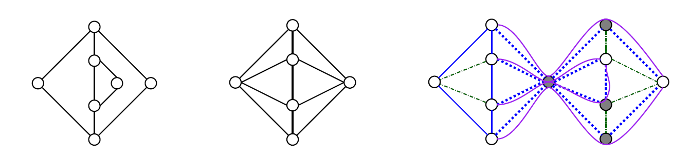
One has to be careful when arguing about the embedding of motif sequences, as illustrated in Figure 1 which shows a counter example for . This means that we typically cannot just incrementally add motif occurrences to discover a certain substructure. This is the motivation for introducing the concept of a dictionary which imposes an order on motif sequences and their attachment points.
3.2 Dictionary Structure and Existence
In a nutshell, a dictionary is a Directed Acyclic Graph (DAG) defined over all possible motifs . and imposes an order (poset relationship ) on problematic motif sequences which need to be embedded one before the other (e.g., the composition depicted in Figure 1). To distinguish them from sequences, dictionary entries are called words.
Definition 5 (Dictionary, Words)
A dictionary is a directed acyclic graph (DAG) over a set of motif sequences together with their attachment points. In the context of the dictionary, we will call a motif sequence word. The links represent the poset embedding relationship .
Concretely, the DAG has a single root , namely the chain graph (with two attachment points). In general, the attachment points of each vertex describing a word define how can be connected to other words. The directed edges represent the transitively reduced embedding poset relation with the chain context: is embeddable in and there is no other word such that , and holds. (The chains before and after the words are added to ensure that attachment points are “used”: there is no edge between two isomorphic words with different attachment point pairs.)
We require that the dictionary be robust to composition: For any node , let denote the “reachable” set of words in the graph and all other words. We require that , where the transitive closure operator denotes an arbitrary sequence (including the empty sequence) of elements in (according to their attachment points).
See Figure 2 for an example. Informally, the robustness requirement means that the word represented by cannot be embedded in any sequence of “smaller” words, unless a subsequence of this sequence is in the dictionary as well. As an example, in a dictionary containing motifs and from Figure 1 would contain vertices , and also , and a path from to .
a)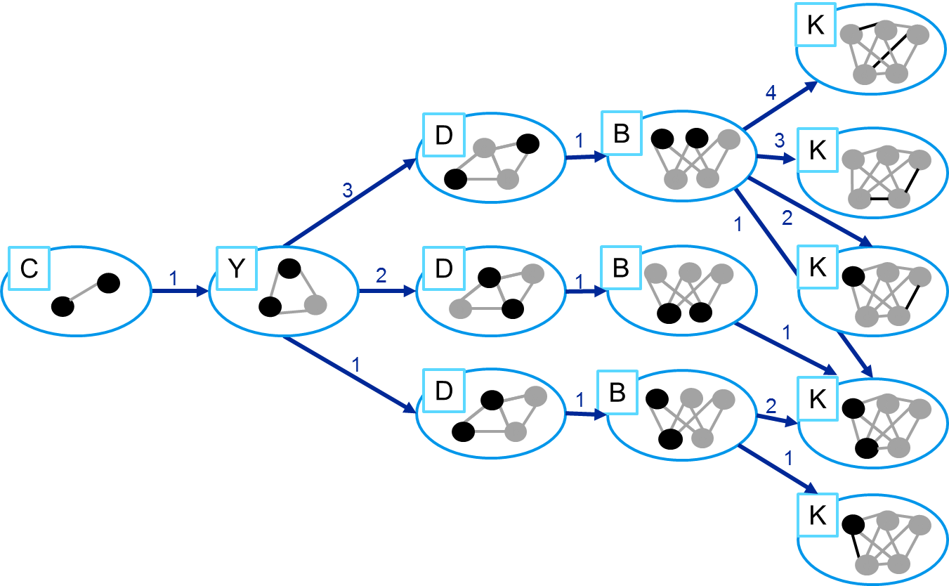 b)
b) 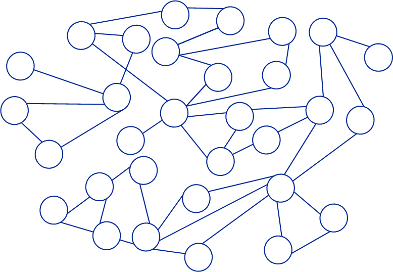
In the following, we use the notation to denote the set of “maximal” vertices with respect to their embeddability into : , where denotes the set of outgoing neighbors of . Furthermore, we say that a dictionary covers a motif sequence iff can be formed by concatenating dictionary words (henceforth denoted by ) at the specified attachment points. More generally, a dictionary covers a graph, if it can be formed by merging sequences of .
Let us now derive some properties of the dictionary which are crucial for a proper substrate topology discovery. First we consider maximal dictionary words which can serve as embedding “anchors” in our algorithm.
Lemma 4
Let be a dictionary covering a sequence of motifs, and let . Then constitutes a subsequence of , i.e., can be decomposed to , and contains no words of order at most , i.e., .
Proof
By contradiction assume and is not a subsequence of (written ). Since covers we have by definition.
Since is a dictionary and we know that . Thus, : has a subsequence of at least one word in . Thus there exists such that . If this implies which contradicts our assumption. Otherwise it means that such that , which contradicts the definition of and thus it must hold that .
The following corollary is a direct consequence of the definition of and Lemma 4: since for a motif sequence with , all the subsequences of that contain no are in . As we will see, the corollary is useful to identify the motif words composing a graph sequence, from the most complex words to the least complex ones.
Corollary 2
Let be a dictionary covering a motif sequence , and let . Then can be decomposed as a sequence with .
This corollary can be applied recursively to describe a motif sequence as a sequence of dictionary entries. Note that a dictionary always exists.
Lemma 5
There exists a dictionary that covers all member graphs of a motif graph family with vertices. [Proof in Appendix]
3.3 The Dictionary Algorithm
With these concepts in mind, we are ready to describe our generalized graph discovery algorithm called Dict (cf Algorithm 1). Basically, Dict always grows a request graph until it is isomorphic to (the graph to be discovered). This graph growing is performed according to the dictionary, i.e., we try to embed new motifs in the order imposed by the dictionary DAG.
Dict is based on the observation that it is very costly to discover additional edges between nodes in a 2-connected component: essentially, finding a single such edge requires testing all possibilities, which is quadratic in the component size. Thus, it is crucial to first explore the basic “knitting” of the topology, i.e., the minors which are at least 2-connected (the motifs). In other words, we maintain the invariant that there are never two nodes which are not -connected in the currently requested graph while they are -connected in ; no path relevant for the connectivity is overlooked and needs to be found later.
Nodes and edges which are not contributing to the connectivity need not be explored at this stage yet, as they can be efficiently added later. Concretely, these additional nodes can then be discovered by (1) using an edge expansion (where additional degree two nodes are added along a motif edge), and by (2) adding “chains” to the nodes (a virtual link constitutes an edge cut of size one and can again be expanded to entire chain of nodes using edge expansion).
Let us specify the topological order in which algorithm Dict discovers the dictionary words. First, for each node in , we define an order on its outgoing edges . This order is sometimes referred to as a “port labeling”, and each path from the dictionary root (the chain ) to a node in can be represented as the sequence of port labels at each traversed node , where corresponds to a port number in . We can simply use the lexicographic order on integers, : , to associate each vertex with its minimal sequence, and sort vertices of according to their embedding order. Let be the rank function associating each vertex with its position in this sorting: (i.e., is the topological ordering of ).
The fact that subsequences can be defined recursively using a dictionary (Lemma 4 and Corollary 2) is exploited by algorithm Dict. Concretely, we apply Corollary 2 to gradually identify the words composing a graph sequence, from the most complex words to the least complex ones. This is achieved by traversing the dictionary depth-first, starting from the root up to a maximal node: algorithm Dict tests the nodes of in increasing port order as defined above. As a shorthand, the word with is written as ; similarly holds if , a notation that will get useful to translate the fact that will be detected before by algorithm Dict. As a consequence, the word of a sequence that gets matched first is uniquely identified: it is : denotes the maximal word in .
Algorithm Dict distinguishes whether the subsequences next to a word are empty () or chains (), and we will refer to the subsequence before by Bf and to the subsequence after by Af. Concretely, while recursively exploring a sequence between two already discovered parts and we check whether the maximal word is directly next to (i.e., ) or or both (), or whether is somewhere in the middle. In the latter case, we add a chain () to be able to find the greatest possible word in a next step.
Dict uses tuples of the form where and , i.e., denotes the maximal word in , is the number of consecutive occurrences of the corresponding word, and Bf and Af represent the words before and after . These tuples are lexicographically ordered by the total order relation on the set of possible tuples defined as follows: let and two such tuples. Then iff or or or .
With these definition we can prove that algorithm Dict is correct.
Theorem 3.1
Given a dictionary for , algorithm Dict correctly discovers any .
Proof
We first prove that the claim is true if forms a motif sequence (without edge expansion). Subsequently, we study the case where the motif sequence is expanded by Rule 2, and finally tackle the general composition case.
Discovery of motif sequences: Due to Lemma 4 it holds that for chosen when Line 1 of is executed for the first time, is partitioned into three subsequences , and . Subsequently is executed on each of the subsequences recursively if , i.e., if the subsequences are not empty. Thus computes a decomposition as described in Corollary 2 recursively. As each of the words used in the decomposition is a subsequence of and does not stop until no more words can be added to any subsequence, it holds that all nodes of will be discovered eventually. In other words, is defined for all .
As a next step we assume to be the sequence of words obtained by Dict to derive a contradiction. Since is the output of algorithm Dict and is hence embeddable in : , there exists a valid embedding mapping . Given , we denote by the set of pairs for which . Now assume that and do not lead to the same resource reservations “”. Hence there are some inconsistencies between the substrate and the output of algorithm Dict: . With each of these “conflict” edges, one can associate the corresponding word (resp. ) in (resp. ). If a given conflict edge spans multiple words, we only consider the words with the highest index as defined by Dict. We also define (resp. )). Since and are by definition not isomorphic, .
Let be the index of the greatest word embeddable on the substrate containing an inconsistency, and be the index of the corresponding word detected by Dict.
() Assume : a lower order motif was erroneously detected. Let (and ) be the set of dictionary entries that are detected before (after) (if any) in by Dict. Observe that the words in were perfectly detected by Dict, otherwise we are in Case (). We can decompose as an alternating sequence of words of and other words using Corollary 2 : with and attachment points and . As the words in are the same in , we can write (using Corollary 2 as well).
Let be the sequence among that contains our misdetected word , and the corresponding sequence in . Observe that since the words cut the sequences of and into subsequences that are embeddable. Observe that since contains it. Note that in the execution of when was detected the higher indexed words had been detected correctly by Dict in previous executions of this subroutine. Hence, and cannot contain any words leading to edges in . Thus which contradicts Line of .
() Now assume : a higher order motif was erroneously detected. Using the same decomposition as step (), we define as the set of words perfectly detected, and therefore decompose and as sequences and with and the property that each .
Let be the sequence among that contains our misdetected word , and the corresponding sequence in . Since , . Thus, since , we deduce which is a contradiction with and Corollary 2.
The same arguments can be applied recursively to show that conflicts in of smaller indices cannot exist either.
Expanded motif sequences. As a next step, we consider graphs that have been extended by applying node insertions (Rule 2) to motif sequences, so called expanded motif sequences: we prove that if is an expanded motif sequence , then algorithm Dict correctly discovers . Given an expanded motif sequence , replacing all two degree nodes with an edge connecting their neighbors unless a cycle of length three would be destroyed, leads to a unique pure motif sequence , . For the corresponding embedding mapping it holds that is exactly the set of removed nodes. Applying to an expanded motif sequence discovers this pure motif sequence by using the nodes in as relay nodes. All nodes in are then discovered in where the reverse operation node insertion is carried out as often as possible. It follows that each node in is either discovered in if it occurs in a motif or in otherwise.
Combining expanded sequences. Finally, it remains to combine the expanded sequences. Clearly, since motifs describe all parts of the graph which are at least 2-connected, the graph remaining after collapsing motifs cannot contain any cycles: it is a tree. However, on this graph Dict behaves like Tree, but instead of attaching chains, entire sequences are attached to different nodes. Along the unique sequence paths between two nodes, Dict fixes the largest words first, and the claim follows by the same arguments as used in the proofs for tree and cactus graphs.
find_motif_sequence()
edge_expansion()
3.4 Request Complexity
The focus of Dict is on generality rather than performance, and indeed, the resulting request complexities can often be high. However, as we will see, there are interesting graph classes which can be solved efficiently.
Let us start with a general complexity analysis. The requests issued by Dict are constructed in Line 1 of and in Line 2 of . We will show that the request complexity of the latter is linear in the number of edges of the host graph while the request complexity of depends on the structure of the dictionary. Essentially, an efficient implementation of Line 1 of in Dict can be seen as the depth-first exploration of the dictionary starting from the chain . More precisely, at a dictionary word requests are issued to see if one of the outgoing neighbors of could be embedded at the position of . As soon as one of the replies is positive, we follow the corresponding edge and continue recursively from there, until no outgoing neighbors can be embedded. Thus, the number of requests issued before we reach a vertex can be determined easily.
Recall that Dict tests vertices of a dictionary according to a fixed port labeling scheme. For any , let be the set of paths from to (each path including and ). In the worst case, discovering costs .
Lemma 6
The request complexity of Line 1 of to find the maximal such that where and is the current request graph is .
Proof
To reach a word in with depth-first traversal there is exactly one path between the chain and . Dict issues a request for at most all the outgoing neighbors of the nodes this path. After has been found, the highest where has to be determined. To this end, another requests are necessary. Thus the maximum of over all word determines the request complexity.
When additional nodes are discovered by a positive reply to an embedding request, then the request complexity between this and the last previous positive reply can be amortized among the newly discovered nodes. Let denote the number of nodes in the motif sequence of the node in the dictionary.
Theorem 3.2
The request complexity of algorithm Dict is at most , where denotes the number of edges of the inferred graph , and is the maximal ratio between the cost of discovering a word in and , i.e., .
Proof
Each time Line 1 of is called, either at least one new node is found or no other node can be embedded between the current sequences (one request is necessary for the latter result). If one or more new nodes are discovered, the request complexity can be amortized by the number of nodes found: If is the maximal word found in Line 1 of then it is responsible for at most requests due to Lemma 6. If it occurs more than once at this position, only one additional request is necessary to discover even more nodes (plus one superfluous request if no more occurrences of can be embedded there). Amortizing the request number over the number of discovered nodes results in requests. All other requests are due to where additional nodes are placed along edges. Clearly, these costs can be amortized by the number of edges in : for each edge , at most two embedding requests are performed (including a “superfluous” request which is needed for termination when no additional nodes can be added).
3.5 Examples
Let us consider concrete examples to provide some intuition for Theorem 3.1 and Theorem 3.2. The execution of Dict for the graph in Figure 2.b), is illustrated in Figure 3.
A fundamental graph class are trees. Since, the tree does not contain any 2-connected structures, it can be described by a single motif: the chain . Indeed, if Dict is executed with a dictionary consisting in the singleton motif set , it is equivalent to a recursive version of Tree from [11] and seeks to compute maximal paths. For the cactus graph, we have two motifs, the request complexity is the same as for the algorithm described in [11].
Corollary 3
Trees can be described by one motif (the chain ), and cactus graphs by two motifs (the chain and the cycle ). The request complexity of Dict on trees and cactus graphs is .
Proof
We present the arguments for cactus graphs only, as trees constitute a subset of the cactus family. The absence of diamond graph minors implies that a cactus graph does not contain two closed faces which share a link. Thus, there can exist at most two different (not even disjoint) paths between any node pair, and the corresponding motif subgraph forms a cycle (or a triangle). Since the cycle has only one attachment point pair, of is constant. Consequently, a linear request complexity follows directly from Theorem 3.2 due to the planarity of cactus graphs (i.e., ).
An example where the dictionary is efficient although the connectivity of the topology can be high are block graphs. A block graph is an undirected graph in which every bi-connected component (a block) is a clique. A generalized block graph is a block graph where the edges of the cliques can contain additional nodes. In other words, in the terminology of our framework, the motifs of generalized block graphs are cliques. For instance, cactus graphs are generalized block graphs where the maximal clique size is three.
Corollary 4
Generalized block graphs can be described by the motif set of cliques. The request complexity of Dict on generalized block graphs is , where denotes the number of edges in the host graph.
Proof
The framework dictionary for generalized block graphs consists of the set of cliques, as a clique with nodes cannot be embedded on sequences of cliques with less than nodes. As there are three attachment point pairs for each complete graph with four or more nodes, Dict can be applied using a dictionary that contains three entries for each motif with more than three nodes (). Thus, the dictionary entry has nodes for and and of is hence in . Consequently the complexity for generalized block graphs is due to Theorem 3.2.
On the other hand, Theorem 3.2 also states that highly connected graphs may require requests, even if the dictionary is small. In the next section, we will study whether this happens in “real world graphs”.
a)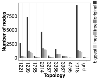 b)
b)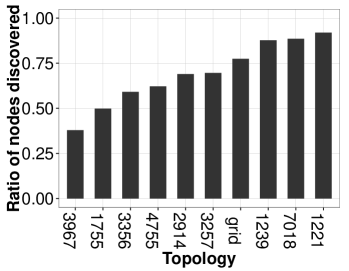 c)
c)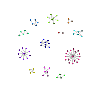 d)
d)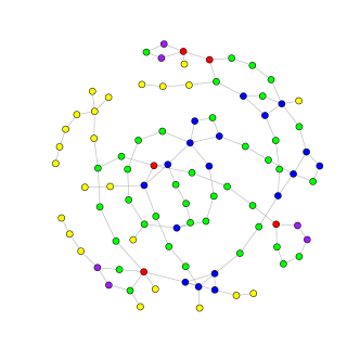
4 Experiments
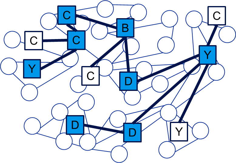
To complement our theoretical results and to validate our framework on realistic graphs, we dissected the ISP topologies provided by the Rocketfuel mapping engine111See http://www.cs.washington.edu/research/networking/rocketfuel/.. In addition, we also dissected the topology of a European electricity distribution grid (grid on the legends). Figure 4 a) provides some statistics about the aforementioned topologies. Since Dict discovers both tree and degree 2 nodes in linear time, this figure shows that most of each topology can be discovered quickly. The inspected topologies are composed of a large bi-connected component (the largest motif), and some other small and simple motifs. Figure 4 b) represents the fraction of each topology that can be discovered by Dict using only a 12-motifs dictionary (see Figure 4 c)). Interestingly, this small dictionary is efficient on different topologies, and contains motifs that are mostly symmetrical. This might stem from the man-engineered origin of the targeted topologies. Finally, Figure 4 d) provides an example of such a topology.
References
- [1] H. Acharya and M. Gouda. On the hardness of topology inference. In Proc. ICDCN, pages 251–262, 2011.
- [2] A. Anandkumar, A. Hassidim, and J. Kelner. Topology discovery of sparse random graphs with few participants. In Proc. SIGMETRICS, 2011.
- [3] N. Bansal, K.-W. Lee, V. Nagarajan, and M. Zafer. Minimum congestion mapping in a cloud. In Proc. 30th PODC, pages 267–276, 2011.
- [4] B. Cheswick, H. Burch, and S. Branigan. Mapping and visualizing the internet. In Proc. USENIX Annual Technical Conference (ATEC), 2000.
- [5] M. K. Chowdhury and R. Boutaba. A survey of network virtualization. Elsevier Computer Networks, 54(5), 2010.
- [6] G. Even, M. Medina, G. Schaffrath, and S. Schmid. Competitive and deterministic embeddings of virtual networks. In Proc. ICDCN, 2012.
- [7] J. Fan and M. H. Ammar. Dynamic topology configuration in service overlay networks: A study of reconfiguration policies. In Proc. IEEE INFOCOM, 2006.
- [8] I. Houidi, W. Louati, and D. Zeghlache. A distributed virtual network mapping algorithm. In Proc. IEEE ICC, 2008.
- [9] J. Lischka and H. Karl. A virtual network mapping algorithm based on subgraph isomorphism detection. In Proc. ACM SIGCOMM VISA, 2009.
- [10] Y. A. Pignolet, G. Tredan, and S. Schmid. Misleading Stars: What Cannot Be Measured in the Internet? In Proc. DISC, 2011.
- [11] Y.-A. Pignolet, G. Tredan, and S. Schmid. Adversarial VNet Embeddings: A Threat for ISPs? In IEEE INFOCOM, 2013.
- [12] G. Schaffrath, S. Schmid, and A. Feldmann. Optimizing long-lived cloudnets with migrations. In Proc. IEEE/ACM UCC, 2012.
- [13] B. Yao, R. Viswanathan, F. Chang, and D. Waddington. Topology inference in the presence of anonymous routers. In Proc. IEEE INFOCOM, pages 353–363, 2003.
- [14] S. Zhang, Z. Qian, J. Wu, and S. Lu. An opportunistic resource sharing and topology-aware mapping framework for virtual networks. In Proc. IEEE INFOCOM, 2012.
Appendix 0.A Appendix
Lemma 1. The embedding relation applied to any family of undirected graphs (short: ), forms a partially ordered set (a poset).
Proof
A poset structure over a set requires that is a (reflexive, transitive, and antisymmetric) order which may or may not be partial. To show that , the embedding order defined over a given set of graphs , is a poset, we examine the three properties in turn.
Reflexive : By using the identity mapping which embeds each node and link to itself, the claim is proved.
Transitive and implies : Let denote the embedding function for and let denote the embedding function for , which must exist by our assumptions. We will show that then also a valid embedding function exists to map to . Regarding the node mapping, we define as , i.e., the result of first mapping the nodes according to and subsequently according to . We first show that is a valid mapping from to as well. First, , maps to a single node in , fulfilling the first condition of the embedding (see Definition 1). Ignoring relay capacities (which is studied together with the conditions on the links below), Condition () of Definition 1 is also fulfilled since the mapping ensures that no node in exceeds its capacity, and can hence safely be mapped to . Let us now turn our attention to the links. We use the following mapping for the edges. Note that maps a single link to an entire (but possibly empty) path in and then maps the corresponding links in to a walk in . We can transform any of these walks into paths by removing cycles; this can only lower the resource costs. Since maps to a subset of only and since can embed all edges of , all link capacities are respected up to relay costs. However, note also that by the mapping and for relay costs , each node can either not be used at all, be fully used as a single endpoint of a link , or serve as a relay for one or more links. Since both end-nodes and relay nodes are mapped to separate nodes in , capacities are respected as well. Conditions () and () hold as well.
Antisymmetric and implies , i.e., and are isomorphic and have the same weights: First observe that if the two networks differ in size, i.e., or , then they cannot be embedded to each other: W.l.o.g., assume , then since nodes of of cannot be split into multiple nodes of (cf Definition 1), there exists a node to which no node from is mapped. This however implies that node must have available capacities to host also , contradicting our assumption that nodes cannot be split in the embedding. Similarly, if , we can obtain a contradiction with the single path argument. Thus, not only the total number of nodes and links in and must be equivalent but also the total amount of node and link resources. So consider a valid embedding for and a valid embedding for , and assume and . It holds that and define an isomorphism between and : Clearly, since , and define a permutation on the vertices. W.l.o.g., consider any link . Then, also : would violate the node capacity constraints in , and requires .
Lemma 5. There exists a dictionary that covers all member graphs of a motif graph family with vertices.
Proof
We present a procedure to construct such a dictionary . Let be the set of all motifs with nodes of the graph family . For each motif with possible attachment point pairs (up to isomorphisms), we add dictionary words to , one for each attachment point pair. The resulting set is denoted by . For each sequence of with at most nodes, we add another word to (with the un-used attachment points of the first and the last subword). There is an edge if the transitive reduction of the embedding relation with context includes an edge between two words. We now prove that is a dictionary, i.e., it is robust to composition. Let . Observe that contains all compositions of words with at most nodes in which can be embedded. Consequently, no matter which sequences are in it holds that cannot be embedded in a sequences in the robustness condition is satisfied. Since has vertices, and since contains all possible motifs of at most vertices, covers .
Note that the proof of Lemma 5 only addresses the composition robustness for sequences of up to nodes. However, it is clear that , and therefore no “mismatch” can happen to happen. Finite dictionaries and with this adapted composition can also be applied in the lemmata proved above, there is only a small notational change necessary in the proof of Lemma 4. (Note that it is always possible to determine the number of nodes by binary search using requests.)