Gaussian Half-Duplex Relay Networks: improved constant gap and connections with the assignment problem

Abstract

This paper considers a general Gaussian relay network where a source transmits a message to a destination with the help of $N$ half-duplex relays. It proves that the information theoretic cut-set upper bound to the capacity can be achieved to within $2.021(N+2)$ bits with noisy network coding, thereby reducing the previously known gap. Further improved gap results are presented for more structured networks like diamond networks.

It is then shown that the generalized Degrees-of-Freedom of a general Gaussian half-duplex relay network is the solution of a linear program, where the coefficients of the linear inequality constraints are proved to be the solution of several linear programs, known in graph theory as the assignment problem, for which efficient numerical algorithms exist. The optimal schedule, that is, the optimal value of the $2^{N}$ possible transmit-receive configurations/states for the relays, is investigated and known results for diamond networks are extended to general relay networks. It is shown, for the case of $2$ relays, that only $3$ out of the $4$ possible states have strictly positive probability. Extensive experimental results show that, for a general $N$-relay network with $N\leq 8$, the optimal schedule has at most $N+1$ states with strictly positive probability. As an extension of a conjecture presented for diamond networks, it is conjectured that this result holds for any HD relay network and any number of relays.

Finally, a $2$-relay network is studied to determine the channel conditions under which selecting the best relay is not optimal, and to highlight the nature of the rate gain due to multiple relays.

I Introduction

Cooperation between nodes in a network has been proposed as a potential and promising technique to enhance the performance of wireless systems in terms of coverage, throughput, network generalized Degrees-of-Freedom (gDoF) and robustness / diversity. This last point is of great importance, especially in military and satellite communications, where redundancy and diversity play a significant role, by insuring a more reliable link between two networks (military communication) and two ground stations (satellite communication), with respect to the point-to-point communication.

The simplest form of collaboration can be modeled as a Relay Channel (RC) [2]. The RC is a multi-terminal network where a source conveys information to a destination with the help of one relay. The relay has no own data to send and its only purpose is to assist the source in the transmission. Motivated by the undeniable practical importance of the RC, in this paper we analyze a system where the communication between a source and a destination is assisted by multiple relays. In particular, we mainly focus on the enhancement in terms of gDoF due to the use of multiple Half-Duplex (HD) relays. A relay is said to work in HD mode if at any time / frequency instant it can not simultaneously transmit and receive. The HD modeling assumption is at present more practical than the Full-Duplex (FD) one. This is so because practical restrictions arise when a node can simultaneously transmit and receive, such as for example how well self-interference can be canceled, making the implementation of FD relays challenging [3, 4].

I-A Related Work

The RC model was first introduced by van der Meulen [5] in 1971. Despite the significant research efforts, the capacity of the general RC is still unknown. In their seminal work [2], Cover and El Gamal proposed a general outer bound, now known as the max-flow min-cut outer bound or cut-set for short, and two achievable schemes: decode-and-forward (DF) and compress-and-forward (CF). The cut-set outer bound was shown to be tight for the degraded RC, the reversely degraded RC and the semi-deterministic RC [2], but it is not tight in general [6].

Although more study has been conducted for FD relays, there are some important references threating HD ones. In [7], the author studied the time-division duplexing RC. Both an outer bound, based on the cut-set argument, and an inner bound, based on partial decode-and-forward (PDF) were developed. In [7], the time instants where the relay switches from listen to transmit and vice versa are assumed fixed, i.e., a priori known by all nodes; we refer to this mode of operation as deterministic switch. In [8], it was shown that higher rates can be achieved by considering a random switch at the relay. In this way the randomness that lies into the switch may be used to transmit (at most one bit per channel use of) further information to the destination. In [8], it was also shown how the memoryless FD framework incorporates the HD one as a special case, and as such there is no need to develop a separate theory for networks with HD relays.

The pioneering work of [2] has been extended to networks with multiple relays. In [9], the authors proposed several inner and outer bounds for FD relay networks as a generalization of DF, CF and the cut-set bound; it was shown that DF achieves the ergodic capacity of a wireless Gaussian network with phase fading if phase information is locally available and the relays are close to the source node.

The exact characterization of the capacity region of a general memoryless network is challenging. Recently it has been advocated that progress can be made towards understanding the capacity by showing that achievable strategies are provably close to (easily computable) outer bounds [10]. As an example, in [11], the authors studied FD Gaussian relay networks with $N+2$ nodes (i.e., $N$ relays, a source and a destination) and showed that the capacity can be achieved to within $\sum_{k=1}^{N+2}5\min\{M_{k},N_{k}\}$ bits with a network generalization of CF named quantize-remap-and-forward (QMF), where $M_{k}$ and $N_{k}$ are the number of transmit and receive antennas, respectively, of node $k$. Interestingly, the gap result remains valid for static and ergodic fading networks where the nodes operate either in FD mode or in HD mode; however [11] did not account for random switch in the outer bound. In [12], the authors demonstrated that the QMF scheme can be realized with nested lattice codes. Moreover they showed that for single antenna HD networks with $N$ relays, by following the approach of [8], i.e., by also accounting for random switch in the outer bound, the gap is $5N$ bits. Recently, for single antenna networks with $N$ FD relays, the $5(N+2)$ bits gap of [11] was reduced to $2\times 0.63(N+2)$ bits (where the factor $2$ accounts for complex-valued inputs) thanks to a novel ingenious generalization of CF named noisy network coding (NNC) [13].

The gap characterization of [13] is valid for a general Gaussian network with FD relays; the gap grows linearly with the number of nodes in the network, which could be a too coarse capacity characterization for networks with a large number of nodes. Smaller gaps can be obtained for more structured networks. For example, a diamond network [14] consists of a source, a destination and $N$ relays where the source and the destination can not communicate directly and the relays can not communicate among themselves. In other words, a general Gaussian relay network with $N$ relays is characterized by $(N+2)(N+1)$ generic channel links, while a diamond network has only $2N$ non-zero channel links. In [14] the case of $N=2$ relays was studied and an achievable region based on time sharing between DF and amplify-and-forward (AF) was proposed. The capacity of a general FD diamond network is known to within $2\log(N+1)$ bits [15]. If, in addition, the FD diamond network is symmetric, that is, all source-relay links are equal and all relay-destination links are equal, the gap is less than 2 bits for any $N$ [16].

HD diamond networks have been studied as well. In a HD diamond network with $N$ relays, there are $2^{N}$ possible combinations of listening / transmitting states, since each relay, at a given time instant, can either transmit or receive. For the case of $N=2$ relays, [17] showed that out of $2^{N}=4$ possible states only $N+1=3$ states suffice to achieve the cut-set upper bound to within less than 4 bits; we refer to the states with strictly positive probability as active states. The achievable scheme of [17] is a clever extension of the two-hop DF strategy of [18]. In [17] a closed-form expression for the aforementioned active states, by assuming no power control and deterministic switch, was derived by solving the dual linear program (LP) associated with the LP derived from the cut-set upper bound. The work in [19] considered a general diamond network with $N=2$ relays and an ‘antisymmetric’ diamond network with $N=3$ relays and showed that a significant fraction of the capacity can be achieved by: (i) selecting a single relay, or (ii) selecting two relays and allowing them to work in a complementary fashion as in [17]. Inspired by [17], the authors of [19] also showed that, for a specific HD diamond network with $N=3$ relays, at most $N+1=4$ states out of the $2^{N}=8$ possible ones are active. The authors also numerically verified that for a general HD diamond network with $N\leq 7$ relays, at most $N+1$ states are active and conjectured that the same holds for any number of relays.

Relay networks were also studied in [20], where an iterative algorithm was proposed to determine the optimal fraction of time each HD relay transmits/receives by using DF under deterministic switching mechanism.

I-B Contributions

In this work we study a general Gaussian HD relay network, whose exact capacity is unknown, by following the approach proposed in [8]. Our main contributions can be summarized as follows:

1. We prove that NNC is optimal to within $2.021(N+2)$ bits. This gap is smaller than the $5N$ bits gap available in the literature [10, 12] for any $N\geq 2$. We also show that the new gap for the HD relay network may be further decreased by considering more structured systems, such as the diamond network, for which the gap is of order $N$.

2. The bounding technique we use is tighter than the one proposed in [13] and, as a by-product of our approach, we reduce the gap for a general multicast complex-valued Gaussian FD network with $K$ nodes from $1.26K$ bits to $1.021K$ bits.

3. In order to determine the gDoF of the channel, one needs to find a tight high-SNR approximation for the different mutual information terms involved in the cut-set upper bound. As a result of independent interest, we show that such tight approximations can be found as the solution of Maximum Weighted Bipartite Matching (MWBM) problems, or assignment problems [21]. The MWBM problem is a special LP for which efficient polynomial-time algorithms, such as the Hungarian algorithm [22], exist. Although not explored here, this technique may be useful in solving other similar problems such as that of finding the gDoF of a general Multiple-Input-Multiple-Output (MIMO) system.

4. We extend the results of [17] from a 2-relay diamond network to a general 2-relay network and we show that, out of the $2^{N}=4$ possible states, at most $N+1=3$ are active. Similarly to the HD diamond network studied in [19], we verify through extensive numerical evaluations that, for a general relay network with $N\leq 8$ relays, at most $N+1$ states are active. Based on this evidence, we conjecture that the conjecture of [19] holds for any HD relay network.

5. We finally consider a general relay network with $N=2$ relays. We highlight under which channel conditions a best-relay selection scheme is strictly suboptimal in terms of gDoF and we gain insight into the nature of the rate gain attainable in networks with multiple relays. For example, we show when the interaction between the relays, which is impossible in diamond networks, increases the gDoF.

I-C Paper Organization

The rest of the paper is organized as follows. Section II describes the channel model and defines the gDoF and the notion of capacity to within a constant gap. Section III shows that the cut-set upper bound and the NNC lower bound for a general Gaussian HD relay network are to within a constant gap from each another. Section IV proves the equivalence between the problem of finding the coefficients of the linear inequality constraints of the LP derived from the cut-set upper bound and the MWBM problem; it also shows that, for a 2-relay network, the number of active states in the cut-set upper bound is at most 3; it finally presents a conjecture regarding the maximum number of active states sufficient to characterize the cut-set upper bound for a general relay network and for any number of relays. Section V provides an example of a HD relay network with $N=2$ relays; it determines under which channel conditions the gDoF achieved with the best-relay selection strategy is strictly smaller than the gDoF attained by exploiting both relays; it provides insights into the synergies of multiple relays. Section VI concludes the paper.

Notation

We use the notation convention of [23]: $[n_{1}:n_{2}]$ is the set of integers from $n_{1}$ to $n_{2}\geq n_{1}$, $[x]^{+}:=\max\{0,x\}$ for $x\in\mathbb{R}$; $Y^{j}$ is a vector of length $j$ with components $(Y_{1},\ldots,Y_{j})$; for an index set $\mathcal{A}$ we let $Y_{\mathcal{A}}=\{Y_{j}:j\in\mathcal{A}\}$; $\mathbf{0}_{j}$ is a column vector of length $j$ of all zeros; $\mathbf{1}_{j}$ is a column vector of length $j$ of all ones; $\mathbf{I}_{j}$ is the identity matrix of dimension $j$; $f_{1}(x)\doteq f_{2}(x)$ means that $\lim_{x\to\infty}f_{1}(x)/f_{2}(x)=1$. $|A|$ indicates the determinant of the matrix $A$ or the cardinality of the set $A$, which one is usually clear from the context, while $\|a\|$ is the Euclidean length of the vector $a$. To indicate a sub matrix of the matrix $\mathbf{A}$ where only the rows indexed by the set $\mathcal{R}$ and the columns indexed by the set $\mathcal{C}$ are retained, we use the Matlab-inspired notation $\mathbf{A}_{\mathcal{R},\mathcal{C}}$. Moreover, for a square matrix $\mathbf{A}$, ${\rm diag}[\mathbf{A}]$ is a vector containing the diagonal elements of $\mathbf{A}$, while for a vector $\mathbf{a}$, ${\rm diag}[\mathbf{a}]$ is a diagonal square matrix with the elements of $\mathbf{a}$ on the main diagonal. $X\sim\mathcal{N}\left(\mu,\sigma^{2}\right)$ indicates that $X$ is a proper-complex random variable distributed normally with mean $\mu$ and variance $\sigma^{2}$.

II System model

II-A General memoryless relay network

A memoryless relay network has one source (node 0), one destination (node $N+1$), and $N$ relays indexed from $1$ to $N$. It consists of $N+1$ input alphabets $\left(\mathcal{X}_{1},\cdots,\mathcal{X}_{N},\mathcal{X}_{N+1}\right)$ (here $\mathcal{X}_{i}$ is the input alphabet of node $i$ except for the source/node 0 where, for notation convenience, we use $\mathcal{X}_{N+1}$ rather than $\mathcal{X}_{0}$), $N+1$ output alphabets $\left(\mathcal{Y}_{1},\cdots,\mathcal{Y}_{N},\mathcal{Y}_{N+1}\right)$ (here $\mathcal{Y}_{i}$ is the output alphabet of node $i$), and a transition probability $\mathbb{P}_{Y_{[1:N+1]}|X_{[1:N+1]}}$. The source has a message $W$ uniformly distributed on $[1:2^{nR}]$ for the destination, where $n$ denotes the codeword length and $R$ the transmission rate in bits per channel use (logarithms are in base $2$). At time $i$, $i\in[1:n]$, the source maps its message $W$ into a channel input symbol $X_{N+1,i}\left(W\right)$, and the $k$-th relay, $k\in[1:N]$, maps its past channel observations into a channel input symbol $X_{k,i}\left(Y_{k}^{i-1}\right)$. The channel is assumed to be memoryless, that is, the following Markov chain holds for all $i\in[1:n]$

$$(W,Y_{[1:N+1]}^{i-1},X_{[1:N+1]}^{i-1})\to X_{[1:N+1],i}\to Y_{[1:N+1],i}.$$

At time $n$, the destination outputs an estimate of the message based on all its channel observations as $\widehat{W}\left(Y_{N+1}^{n}\right)$. The capacity is the largest nonnegative rate such that $\mathbb{P}[\widehat{W}\!\neq\!W]\rightarrow 0$ as $n\!\rightarrow\!+\infty$.

In this general memoryless framework, each relay can listen and transmit at the same time, i.e., it is a FD node. HD channels are a special case of the memoryless FD framework in the following sense [8]. With a slight abuse of notation compared to the previous paragraph, we let the channel input of the $k$-th relay, $k\in[1:N]$, be the pair $(X_{k},S_{k})$, where $X_{k}\in\mathcal{X}_{k}$ as before and $S_{k}\in\{0,1\}$ is the state random variable that indicates whether the $k$-th relay is in receive-mode ($S_{k}=0$) or in transmit-mode ($S_{k}=1$). In the HD case the transition probability is specified as $\mathbb{P}_{Y_{[1:N+1]}|X_{[1:N+1]},S_{[1:N]}}$.

II-B The Gaussian HD relay network

The single-antenna complex-valued power-constrained Gaussian HD relay network is described by the input/output relationship

$$\mathbf{Y}=\mathbf{H}_{\rm eq}\mathbf{X}+\mathbf{Z},$$ (1a)

$$\mathbf{H}_{\rm eq}:=\begin{bmatrix}\mathbf{I}_{N}-\mathrm{diag}[\mathbf{S}]&\mathbf{0}_{N}\\ \mathbf{0}_{N}^{T}&1\\ \end{bmatrix}\ \mathbf{H}\ \begin{bmatrix}\mathrm{diag}[\mathbf{S}]&\mathbf{0}_{N}\\ \mathbf{0}_{N}^{T}&1\\ \end{bmatrix}$$ (1b)

where

• $\mathbf{Y}:=[Y_{1},\ldots,Y_{N},Y_{N+1}]^{T}\in\mathbb{C}^{N+1}$ is the vector of the received signals.

• $\mathbf{X}:=[X_{1},\ldots,X_{N},X_{N+1}]^{T}\in\mathbb{C}^{N+1}$ is the vector of the transmitted signals (recall that, although the source is referred to as node 0, its input is indicated as $X_{N+1}$ rather than $X_{0}$). Without loss of generality, we assume that the channel inputs are subject to the average power constraint $\mathbb{E}\left[|X_{k}|^{2}\right]\leq 1$, $k\in[1:N+1]$.

• $\mathbf{S}:=[S_{1},\ldots,S_{N}]\in\{0,1\}^{N}$ is the vector of the binary relay states, which takes into account if the $k$-th relay is receiving ($S_{k}=0$) or transmitting ($S_{k}=1$) for $k\in[1:N]$.

• $\mathbf{H}\in\mathbb{C}^{(N+1)\times(N+1)}$ is the constant channel matrix known by all terminals defined as

  $$\mathbf{H}:=\begin{bmatrix}\mathbf{H}_{\rm r\to r}&\mathbf{H}_{\rm s\to r}\\ \mathbf{H}_{\rm r\to d}&\mathbf{H}_{\rm s\to d}\\ \end{bmatrix}.$$ (2)

  The entry in position $(i,j)$ of the channel matrix in (2) represents the channel from node $j$ to node $i$, $(i,j)\in[1:N+1]^{2}$, in particular:

  • $\mathbf{H}_{\rm r\to r}\in\mathbb{C}^{N\times N}$ defines the network connections among relays, i.e., $[\mathbf{H}_{\rm r\to r}]_{ij}$, $(i,j)\in[1:N]^{2}$, is the channel gain from the $j$-th relay to the $i$-th relay. Notice that the entries on the main diagonal of $\mathbf{H}_{\rm r\to r}$ do not matter for channel capacity, since the $k$-th relay, $k\in[1:N]$ can remove the ‘self-interference’ $X_{k}$ from $Y_{k}$.

  • $\mathbf{H}_{\rm s\to r}\in\mathbb{C}^{N\times 1}$ is the column vector which contains the channel gains from the source to the relays, i.e., $[\mathbf{H}_{\rm s\to r}]_{i,1}$, $i\in[1:N]$, is the channel gain from the source to the $i$-th relay;

  • $\mathbf{H}_{\rm r\to d}\in\mathbb{C}^{1\times N}$ is the row vector which contains the channel gains from the relays to the destination, i.e., $[\mathbf{H}_{\rm r\to d}]_{1,i}$, $i\in[1:N]$, is the channel gain from the $i$-th relay to the destination;

  • $\mathbf{H}_{\rm s\to d}\in\mathbb{C}^{1\times 1}$is the channel gain between the source and the destination (recall that by our notation the source input is indicated as $X_{N+1}$ rather than $X_{0}$).

• $\mathbf{Z}:=[Z_{1},\ldots,Z_{N},Z_{N+1}]^{T}\in\mathbb{C}^{N+1}$ is the jointly Gaussian noise vector. Without loss of generality, the noises are assumed to have zero mean and unit variance. Furthermore we assume, not without loss of generality [24], that the noises are independent, i.e., the covariance of $\mathbf{Z}$ is the identity matrix.

The capacity of the Gaussian HD relay network in (1) is not known in general. In order to evaluate the ultimate performance of this system we make use of two metrics: the gDoF and the capacity to within a constant gap. The capacity to within a constant gap is defined as:

Definition 1.

The capacity $\mathsf{C}$ of the Gaussian HD relay network in (1) is said to be known to within $\mathsf{GAP}$ bits if one can show an achievable rate $R^{\rm(in)}$ and an outer bound $R^{\rm(out)}$ such that

$$R^{\rm(in)}\leq\mathsf{C}\leq R^{\rm(out)}\leq R^{\rm(in)}+\mathsf{GAP},$$ (3)

where $\mathsf{GAP}$ is a constant that does not depend on the channel gain matrix $\mathbf{H}$ in (1).

Knowing the capacity to within a constant gap implies the exact knowledge of the gDoF defined as:

Definition 2.

The gDoF of the Gaussian HD relay network in (1) is defined as

$$\mathsf{d} :=\lim_{\mathsf{SNR}\to+\infty}\frac{\mathsf{C}}{\log(1+\mathsf{SNR})},$$ (4)

where $\mathsf{C}$ is the capacity and $\mathsf{SNR}\in\mathbb{R}^{+}$ parameterizes the channel gains as $|h_{ij}|^{2}=\mathsf{SNR}^{\beta_{ij}}$, for some non-negative $\beta_{ij}$, $(i,j)\in[1:N+1]^{2}$.

The gDoF in (4) is an exact characterization of the capacity at high-SNR, while the capacity to within a constant gap in (3) quantifies how far inner and outer bounds are in the worst $\mathsf{SNR}$ scenario.

III Capacity to within a constant gap

This section is devoted to the capacity characterization of the Gaussian HD relay network in (1) to within a constant gap. To accomplish this, we first adapt the cut-set upper bound [9] and the NNC lower bound [13] to the HD case by following the approach proposed in [8]. Then we show that these bounds are at most a constant number of bits apart. Our result is:

Theorem 1.

The cut-set upper bound for the HD relay network with $N$ relays is achievable to within

$$\mathsf{GAP}\leq 2.021(N+2)\ \rm{bits},$$ (5)

by using as achievable scheme NNC with deterministic switch.

Proof:

Here we prove a general gap result for multicast single-antenna complex-valued power-constrained Gaussian HD networks in the spirit of [13, Theorem 4]. The channel model is defined as in the Section II-B except that each node $k\in[1:K]$ has an independent message of rate $R_{k}$ for the nodes indexed by $\mathcal{D}\not=\emptyset$ so that the channel input/output relationship reads $\mathbf{Y}=(\mathbf{I}_{K}-\mathbf{S})\ \mathbf{H}\ \mathbf{S}\ \mathbf{X}+\mathbf{Z}$. The gap for a HD relay network with $N$ relays is a special case of this setup for $K=N+2$.

The capacity of a HD Gaussian multicast network can be lower bounded by adapting the NNC scheme for the general memoryless network [13] to the HD case by following [8]. For each $\mathcal{A}\subseteq[1:K]\backslash\emptyset$ and such that $\mathcal{A}^{c}\cap\mathcal{D}\not=\emptyset$, similarly to [13, eq.(20)], the NNC lower bound gives

$$\sum_{i\in\mathcal{A}}R_{i} \geq I(X_{\mathcal{A}};\widehat{Y}_{\mathcal{A}^{c}}|X_{\mathcal{A}^{c}},S_{[1:K]})-I(Y_{\mathcal{A}};\widehat{Y}_{\mathcal{A}}|\widehat{Y}_{\mathcal{A}^{c}},X_{[1:K]},S_{[1:K]})$$

$$\geq\sum_{s=1}^{2^{K}}\lambda_{s}\ \log\left|\mathbf{I}_{|\mathcal{A}^{c}|}+\frac{1}{1+\sigma^{2}}\ \mathbf{H}_{\mathcal{A},s}\mathbf{H}_{\mathcal{A},s}^{H}\right|-|\mathcal{A}|\log\left(1+\frac{1}{\sigma^{2}}\right),$$ (6)

where $\lambda_{s}:=\mathbb{P}[S_{[1:K]}=s]\in[0,1],\forall s\in[1:2^{K}]:\ \sum_{s=1}^{2^{K}}\lambda_{s}=1$, where “$S_{[1:K]}=s$” is a shorthand notation for $S_{[1:K]}=[S_{1},\ldots,S_{K}]$ where $S_{k}\in[0:1],\ \forall k\in[1:K],$ are such that $s=1+\sum_{k=1}^{K}S_{k}2^{K-k}$ (for example “$S_{[1:5]}=8$” means $S_{[1:5]}=[S_{1},\ldots,S_{5}]=[0,0,1,1,1]$ since $8-1=0\cdot 2^{4}+0\cdot 2^{3}+1\cdot 2^{2}+1\cdot 2^{1}+1\cdot 2^{0}$; similarly ${\rm diag}[s]|_{s=8}={\rm diag}\big{[}[0,0,1,1,1]\big{]}$). The matrix $\mathbf{H}_{\mathcal{A},s}$ is defined as $\mathbf{H}_{\mathcal{A},s}:=\big{[}(\mathbf{I}_{K}-{\rm diag}[s])\ \mathbf{H}\ {\rm diag}[s]\big{]}_{\mathcal{A}^{c},\mathcal{A}}$. In all states $s\in[1:2^{K}]$, we consider i.i.d. $\mathcal{N}\left(0,1\right)$ inputs, time sharing random variable $Q$ set to $Q=S_{[1:K]}$ (with this choice the nodes can coordinate), and compressed output $\widehat{Y}_{k}:=Y_{k}+\widehat{Z}_{k}$, $k\in[1:K]$, for $\widehat{Z}_{k}\sim\mathcal{N}(0,\sigma^{2})$ independent of all other random variables (note that the variance of $\widehat{Z}_{k}$ does not depend on the user index $k$).

The cut-set upper bound in [9] adapted to the HD case [8] gives, similarly to [13, eq.(19)],

$$\sum_{i\in\mathcal{A}}R_{i} \leq I(X_{\mathcal{A}},S_{\mathcal{A}};Y_{\mathcal{A}^{c}}|X_{\mathcal{A}^{c}},S_{\mathcal{A}^{c}})$$

$$\leq I(S_{\mathcal{A}};Y_{\mathcal{A}^{c}})+I(X_{\mathcal{A}};Y_{\mathcal{A}^{c}}|X_{\mathcal{A}^{c}},S_{[1:K]})$$

$$\leq H(S_{\mathcal{A}})+\sum_{s=1}^{2^{K}}\lambda_{s}\ \log\left|\mathbf{I}_{|\mathcal{A}^{c}|}+\mathbf{H}_{\mathcal{A},s}\mathbf{K}_{\mathcal{A},s}\mathbf{H}_{\mathcal{A},s}^{H}\right|$$

$$\stackrel{{\scriptstyle\rm(a)}}{{\leq}}|\mathcal{A}|\log(2)+\sum_{s=1}^{2^{K}}\lambda_{s}\ \log\left|\mathbf{I}_{|\mathcal{A}^{c}|}+\frac{1}{1+\sigma^{2}}\mathbf{H}_{\mathcal{A},s}\mathbf{H}_{\mathcal{A},s}^{H}\right|$$

$$\quad+\sum_{s=1}^{2^{K}}\lambda_{s}{\rm Rank}[\mathbf{H}_{\mathcal{A},s}]\log\left(\mathrm{e}\max\left\{1,\frac{1+\sigma^{2}}{\mathrm{e}}\ \frac{|\mathcal{A}|}{{\rm Rank}[\mathbf{H}_{\mathcal{A},s}]}\right\}\right)^{\min\left\{\frac{1+\sigma^{2}}{\mathrm{e}},\frac{{\rm Rank}[\mathbf{H}_{\mathcal{A},s}]}{|\mathcal{A}|}\right\}}$$

$$\stackrel{{\scriptstyle\rm(b)}}{{\leq}}|\mathcal{A}|\log(2)+\sum_{s=1}^{2^{K}}\lambda_{s}\ \log\left|\mathbf{I}_{|\mathcal{A}^{c}|}+\frac{1}{1+\sigma^{2}}\mathbf{H}_{\mathcal{A},s}\mathbf{H}_{\mathcal{A},s}^{H}\right|$$

$$\quad+\!\min\{|\mathcal{A}|,|\mathcal{A}^{c}|\}\log\left(\mathrm{e}\max\left\{1,\frac{1\!+\!\sigma^{2}}{\mathrm{e}}\ \frac{|\mathcal{A}|}{\min\{|\mathcal{A}|,|\mathcal{A}^{c}|\}}\right\}\right)^{\min\left\{\frac{1\!+\!\sigma^{2}}{\mathrm{e}},\frac{\min\{|\mathcal{A}|,|\mathcal{A}^{c}|\}}{|\mathcal{A}|}\right\}},$$ (7)

for all $\mathcal{A}\subseteq[1:K]\backslash\emptyset$ and such that $\mathcal{A}^{c}\cap\mathcal{D}\not=\emptyset$ (see  [13, eq.(4)]), where $\mathbf{K}_{\mathcal{A},s}$ represents the covariance matrix of $X_{\mathcal{A}}$ conditioned on $S_{[1:K]}=s$. The inequality in (a) follows since the entropy of a random variable can be upper bounded with the support of the variable and by using [13, Lemma 1] for some $\sigma^{2}\geq\mathrm{e}-2$. The inequality in (b) is due to the fact that the function is increasing with respect to the rank of the channel matrix and the rank is upper bounded by the minimum between the number of rows and of columns.

By letting $\gamma=1+\sigma^{2}\geq\mathrm{e}-1$ and $\mu=\frac{|\mathcal{A}|}{K}$, the gap between the cut-set upper bound in (7) and the NNC lower bound in (6) becomes

$$\mathsf{GAP} \leq K\left(\min_{\gamma\geq\mathrm{e}-1}\max_{\mu\in[0:1]}\left\{\mu\log\left(\frac{2\gamma}{\gamma-1}\right)\right.\right.+$$

$$\left.\left.+\min\left\{\mu,1-\mu\right\}\min\left\{\frac{\gamma}{\mathrm{e}},\frac{\min\{\mu,1-\mu\}}{\mu}\right\}\log\left(\max\left\{\mathrm{e},\frac{\gamma\mu}{\min\{\mu,1-\mu\}}\right\}\right)\right\}\right)$$

$$\stackrel{{\scriptstyle\rm(c)}}{{=}}\frac{K}{2}\left(\min_{\gamma\geq\mathrm{e}-1}\left\{\log\left(\frac{2\gamma}{\gamma-1}\right)+\min\left\{\frac{\gamma}{\mathrm{e}},1\right\}\log\left(\mathrm{e}\max\left\{1,\frac{\gamma}{\mathrm{e}}\right\}\right)\right\}\right)$$

$$\stackrel{{\scriptstyle\rm(d)}}{{=}}2.021K\ \text{bits},$$

where the maximum over $\mu\in[0,1]$ is attained at $\mu^{\rm{opt}}=\frac{1}{2}$ and the minimum over $\gamma$ is attained at $\gamma^{\rm{opt}}=\frac{\sqrt{4\mathrm{e}+1}+1}{2}$ and these results lead to the equalities in (c) and (d), respectively. ∎

We observe that the gap in (5) improves, for any number of relays greater than one, on the previously known gap result of $5N\ \rm{bits}$ [12]. Moreover:

Remark 1.

The gap result in (5) for $N\!=\!1$ gives $\mathsf{GAP}\!\leq\!6.0630$ bits, which is greater than the 1.61 bits gap we found for the single relay case in [25]. This is due to the fact that the bounding steps in the special case of $N\!=\!1$ are tighter than those we used here for a general $N$.

Note also that for a single relay, PDF is optimal to within 1 bit [25]. However, PDF does not seem to be easily extendable to networks with an arbitrary number of relays [9], which is the main motivation for considering NNC here.

Remark 2.

In a preliminary version of this work [1], by using a bounding technique as in [26, pages 20-5, 20-7] we obtained

$$\mathsf{GAP}\cong\frac{N+2}{2}\log\left(4(N+2)\right)\ \rm{bits}.$$ (8)

As shown in Fig. 1 the gap in (5) is smaller that the one in (8) for $N\geq 2$. This is accomplished thanks to the tighter bound from [13, Lemma 1].

Remark 3.

From [13], the gap of a general $K$-user multicast complex-valued FD Gaussian network is $(2\times 0.63)K$. However, by using the tighter bound ${\rm Rank}[\mathbf{H}_{\mathcal{A},s}]\leq\min\{|\mathcal{A}|,|\mathcal{A}^{c}|\}$, instead of ${\rm Rank}[\mathbf{H}_{\mathcal{A},s}]\leq|\mathcal{A}|$, the gap can be reduced to $(2\times 0.5105)K$.

A smaller gap than the one in (5) may be obtained by deriving tighter bounds on specific network topologies. For example, in [15] it was found that for a Gaussian FD diamond network with $N$ relays the gap is of the order $\log(N)$, rather than linear in $N$ [13]. Moreover, for a symmetric FD diamond network with $N$ relays the gap does not depend on the number of relays and it is upper bounded by 2 bits [16]. The key difference between a general relay network and a diamond network is that for each subset $\mathcal{A}$ we have ${\rm Rank}[\mathbf{H}_{\mathcal{A}}]\leq 2$, i.e., the rank of any channel sub-matrix does no longer depend on the cardinality of the index set $\mathcal{A}$. Based on the simpler topology of a diamond network we have:

Proposition 1.

The cut-set upper bound for the Gaussian HD diamond network with $N$ relays is achievable to within

$$\mathsf{GAP}\leq\frac{4}{N+2}\log\left(\frac{N+2}{2}+\frac{(N+2)^{3}}{8}\right)+(N+2)\log\left(2+\frac{8}{(N+2)^{2}}\right)$$ (9)

bits.

Proof:

The proof can be found in Appendix A. ∎

When $N\gg 1$, the gap in (9) can be approximated as $\mathsf{GAP}\cong N\ \rm{bits}$. As expected, the gap in (9) for the HD diamond network is in general (for $N\geq 3$) smaller than that in (5) computed for the general HD relay network; this is in line with what happens in the FD case. However, in FD for the diamond network the gap is logarithmic in $N$ [15], while the gap in (9) still grows linearly with $N$. This is in part due to the fact that, in the HD outer bound, there is an entropy term due to the random switch that is maximized by considering a uniform probability over the all possible listen / transmit states that, for the multicast network, are $2^{N+2}$ (see Appendix A).

As we shall see in the next section, for a general HD network with $N$ relays, only $N+1$ states, out of the possible $2^{N}$ states, appear to be needed to characterize the cut-set upper bound. It is subject of current investigation on how to use this observation to develop bounds leading to a smaller gap.

IV Analysis of the optimal schedule

In general, for a $N$-relay network, $2^{N}$ states are possible. A capacity achieving scheme must optimize the fraction of time each of these states occurs. In [17], it was proved that for a diamond network with $N=2$ relays, out of the $2^{N}=4$ possible states, at most $N+1=3$ have a non-zero probability and are sufficient to characterize the cut-set upper bound, i.e., we say that there are $N+1=3$ active states. In [19], the authors extended the result of [17] to a special case of diamond network with $N=3$ relays; based on numerical evidences, [19] conjectured that for a $N$-relay diamond network out of the $2^{N}$ possible states at most $N+1$ states are active. Here we extend these results to a general Gaussian HD relay network as follows. The claim “out of $2^{N}$ possible states only $N+1$ states are active as far as gDoF is concerned” is proved analytically for $N=2$, shown to hold by numerical evaluations for $N\leq 8$ and conjectured to hold for any $N$. If the conjecture were true, it would show that HD relay networks have intrinsic properties regardless of their topology, i.e., known results for diamond networks are not a consequence of the simplified network topology.

In order to determine the gDoF we must find a tight high-SNR approximation for the different MIMO-type mutual information terms involved in the cut-set upper bound (see Section III eq.(7)). As a result of independent interest, besides the application to the Gaussian HD relay network studied in this paper, we first show that such an approximation can be found as the solution of a Maximum Weighted Bipartite Matching (MWBM) problem.

IV-A The maximum weighted bipartite matching (MWBM) problem

In graph theory, a weighted bipartite graph, or bigraph, is a graph whose vertices can be separated into two sets such that each edge in the graph has exactly one endpoint in each set. Moreover, a non-negative weight is associated with each edge in the bigraph [27]. A matching, or independent edge set, is a set of edges without common vertices [27]. The MWBM problem, or assignment problem, is defined as a matching where the sum of the edge weights in the matching has the maximal value [21]. The Hungarian algorithm is a polynomial time algorithm that efficiently solves the assignment problem [22]. Equipped with these definitions, we now show the following high-SNR approximation of the MIMO capacity:

Theorem 2.

Let $\mathbf{H}\in\mathbb{R}^{k\times n}$ be a full-rank matrix, where without loss of generality $k\leq n$. Let $\mathcal{S}_{n,k}$ be the set of all $k$-combinations of the integers in $[1:n]$ and $\mathcal{P}_{n,k}$ be the set of all $k$-permutations of the integers in $[1:n]$. Then,

$$|\mathbf{I}_{k}+\mathbf{H}\mathbf{H}^{H}| =\sum_{\varsigma\in\mathcal{S}_{n,k}}\sum_{\pi\in\mathcal{P}_{n,k}}\underbrace{\prod_{i=1}^{k}|h_{i,\pi(i)}|^{2}}_{=\mathsf{SNR}^{\sum_{i=1}^{k}[\mathbf{B}_{\varsigma}]_{i,\pi(i)}}}+\quad T\doteq\mathsf{SNR}^{\text{MWBM}(\mathbf{B})},$$ (10)

$$\text{MWBM}(\mathbf{B}):={\max_{\varsigma\in\mathcal{S}_{n,k}}\max_{\pi\in\mathcal{P}_{n,k}}\sum_{i=1}^{k}\left[\mathbf{B}_{\varsigma}\right]_{i,\pi(i)}},$$ (11)

where $\mathbf{B}$ is the SNR-exponent matrix defined as $[\mathbf{B}]_{ij}=\beta_{ij}\geq 0:|h_{ij}|^{2}=\mathsf{SNR}^{\beta_{ij}}$, $\mathbf{B}_{\varsigma}$ is the square matrix obtained from $\mathbf{B}$ by retaining all rows and those columns indexed by $\varsigma$, and $T$ is the sum of terms that overall have an exponential behavior that is less than $\text{MWBM}(\mathbf{B})$.

Proof:

The proof can be found in Appendix B. The expression in (11) is a possible way of writing the MWBM problem. ∎

Theorem 2 establishes an interesting connection between the capacity of a MIMO channel (with independent inputs) and graph theory. Note that the high-SNR expression found in Theorem 2 holds for correlated inputs as well, as long as the average power constraint is a finite constant. More importantly, Theorem 2 allows to move from DoF, where all exponents $\beta_{ij}$ have the same value, to gDoF, where different channel gains have different exponential behavior. DoF is essentially a characterization of the rank of the channel matrix; gDoF captures the potential advantage due to ‘asymmetric’ channel gains. gDoF, to the best of our knowledge, has been investigated so far only for Single-Input-Single-Output (SISO) networks with very few number of nodes; we believe that the reason is that in these cases one has only to consider equivalent Multiple-Input-Single-Output (MISO) and Single-Input-Multiple-Output (SIMO) channels, or to explicitly deal with determinants of matrices with small dimensions. Our result extends the gDoF analysis to any MIMO channel as we explain through some examples:

1. Case $k=1\leq n$: In a MISO or SIMO channel, with channel vector $\mathbf{h}:=[h_{1},\ldots,h_{n}]$ such that $|h_{k}|^{2}=\mathsf{SNR}^{\beta_{k}},k\in[1:n]$, one trivially has

   $$\log(1+||\mathbf{h}||^{2})=\log\left(1+\sum_{i=1}^{n}\mathsf{SNR}^{\beta_{i}}\right)\stackrel{{\scriptstyle\mathsf{SNR}\gg 1}}{{\doteq}}\log\left(\mathsf{SNR}^{\max_{i\in[1:n]}\{\beta_{i}\}}\right).$$

   The corresponding MWBM problem has one set of vertices $\mathcal{A}_{1}$ consisting of $k=|\mathcal{A}_{1}|=1$ node and the other set of vertices $\mathcal{A}_{2}$ consisting of $n=|\mathcal{A}_{2}|\geq 1$ nodes. The weights of the edges connecting the single vertex in $\mathcal{A}_{1}$ to the $n$ vertices in $\mathcal{A}_{2}$ can be represented as the non-negative vector $\mathbf{B}=[\beta_{1},\ldots,\beta_{n}]$. Clearly, the optimal $\text{MWBM}(\mathbf{B})=\max_{i\in[1:n]}\{\beta_{i}\}$ assigns the single vertex in $\mathcal{A}_{1}$ to the vertex in $\mathcal{A}_{2}$ that is connected to it through the edge with the maximum weight.

2. Case $k=n=2$: As another example from the 2-user interference channel literature, consider the cut-set sum-rate upper bound [28]

   $$\log\left(\mathbf{I}_{2}+\mathbf{H}\mathbf{H}^{H}\right)\stackrel{{\scriptstyle\mathsf{SNR}\gg 1}}{{\doteq}}\log\left(\mathsf{SNR}^{\max\{\beta_{13}+\beta_{24},\beta_{23}+\beta_{14}\}}\right),$$

   $$\quad\mathbf{H}:=\begin{bmatrix}h_{13}&h_{23}\\ h_{14}&h_{24}\\ \end{bmatrix}=\begin{bmatrix}\mathsf{SNR}^{\beta_{13}/2}\ \mathrm{e}^{\mathrm{j}\theta_{13}}&\mathsf{SNR}^{\beta_{23}/2}\ \mathrm{e}^{\mathrm{j}\theta_{23}}\\ \mathsf{SNR}^{\beta_{14}/2}\ \mathrm{e}^{\mathrm{j}\theta_{14}}&\mathsf{SNR}^{\beta_{24}/2}\ \mathrm{e}^{\mathrm{j}\theta_{24}}\\ \end{bmatrix}.$$

   The corresponding MWBM problem has one set of vertices $\mathcal{A}_{1}$ consisting of $k=|\mathcal{A}_{1}|=2$ nodes (for future references let us refer to these vertices as nodes 1 and 2 – see first subscript in the channel gains) and the other set of vertices $\mathcal{A}_{2}$ consisting also of $n=|\mathcal{A}_{2}|=2$ nodes (for future references let us refer to these vertices as nodes 3 and 4 – see second subscript in the channel gains). The weights of the edges connecting the vertices in $\mathcal{A}_{1}$ to the vertices in $\mathcal{A}_{2}$ can be represented as the non-negative weights $\beta_{ji},\ i=3,4,\ j=1,2$. In this example, one possible matching assigns node 1 to node 3 and node 2 to node 4 (giving total weight $\beta_{13}+\beta_{24}$), while the other possible matching assigns node 2 to node 3 and node 1 to node 4 (giving total weight $\beta_{23}+\beta_{14}$); the best assignment is the one that gives the largest total weight.

   Notice that the MWBM is a tight approximation of the $2\times 2$ MIMO capacity only when the channel matrix is full rank, see [28, eq.(5) 1st line], but it is loose when the channel matrix is rank deficient, see [28, eq.(5) 2nd line, and compare with eq.(11)]. The reason is that the MWBM can not capture the impact of phases in MIMO situations. To exclude the case of a rank deficient channel matrix from our general setting for any value of $k$ and $n$, we may proceed as in [29, page 2925]. Namely, we pose a reasonable distribution, such as for example the i.i.d. uniform distribution, on the phases $\theta_{ji},\ i=3,4,\ j=1,2$, so that almost surely the channel matrix is full rank.

3. Case $k=2,n=3$: The MWBM allows to find the high-SNR approximation of any MIMO system capacity. As an example, which to the best of our knowledge is not known from the literature, consider a full-rank MIMO systems $n=3$ transmit antennas and $k=2$ receive antennas and with SNR-exponent matrix $\mathbf{B}=\begin{bmatrix}\beta_{11}&\beta_{12}&\beta_{13}\\ \beta_{21}&\beta_{22}&\beta_{23}\\ \end{bmatrix}$. In this case we have

   $$\text{MWBM}(\mathbf{B})=\max\Big{\{}\beta_{11}+\beta_{22},\beta_{11}+\beta_{23},\beta_{12}+\beta_{21},\beta_{12}+\beta_{23},\beta_{13}+\beta_{21},\beta_{13}+\beta_{22}\Big{\}},$$

   which can also be obtained by tedious direct computation of the limiting value of the corresponding log-det formula.

IV-B The gDoF for a general $N$-relay network

With Theorem 2 we can now express the gDoF $\mathsf{d}$ in (4) of the Gaussian HD relay network in (1) as a LP. In particular, let

$$\mathbf{f}^{T} :=[\mathbf{0}^{T}_{2^{N}},1]$$ (12a)

$$\mathbf{x}^{T} :=[\lambda_{1},\ldots,\lambda_{2^{N}},\mathsf{d}],$$ (12b)

then

$$\mathsf{d} =\max\{\mathbf{f}^{T}\ \mathbf{x}\}$$ (12c)

$$\mathrm{s.t.}\begin{bmatrix}-\mathbf{A}&\mathbf{1}_{2^{N}}\\ \mathbf{1}_{2^{N}}^{T}&0\\ \end{bmatrix}\mathbf{x}\leq\mathbf{f},\quad\mathbf{x}\geq 0,$$ (12d)

where the non-negative matrix $$\mathbf{A}\in\mathbb{R}^{2^{N}\times 2^{N}} X_{N+1} X_{0}$$ has entries (recall that, although the source is referred to as node 0, its input is indicated as rather than )

$$[\mathbf{A}]_{ij} :=\lim_{\mathsf{SNR}\to+\infty}\frac{I(X_{\mathcal{A}_{i}\cup\{N+1\}};Y_{\mathcal{A}_{i}^{c}\cup\{N+1\}}|X_{\mathcal{A}_{i}^{c}},S_{[1:N]}=s_{j})}{\log(1+\mathsf{SNR})}.$$ (12e)

By a simple application of Theorem 2 we have

Theorem 3.

$[\mathbf{A}]_{ij}=\text{MWBM}(\mathbf{B}_{\mathcal{A}_{i},s_{j}})$.

The notation in eq.(12e) and in Theorem 3 is as follows. $\mathbf{B}$ indicates the SNR-exponent matrix defined as $[\mathbf{B}]_{ij}=\beta_{ij}\geq 0:|h_{ij}|^{2}=\mathsf{SNR}^{\beta_{ij}}$ (defined in (2)), and the indices $(i,j)$ have the following meaning. Index $i$ refers to a “cut” in the network and index $j$ to a “state of the relays”. Both indices range in $[1:2^{N}]$ and must be seen as the decimal representation of a binary number with $N$ bits. $\mathcal{A}_{i}$, $i\in[1:2^{N}]$, is the set of those relays who have a one in the corresponding binary representation of $i-1$ (example for $N=3$: for $i-1=6=1\cdot 2^{2}+1\cdot 2^{1}+0\cdot 2^{0}$ we have $\mathcal{A}_{7}=\{1,2\}$ and therefore $\mathcal{A}_{7}^{c}=\{3\}$). $s_{j}$, $j\in[1:2^{N}]$, sets the state of a relay to the corresponding bit in the binary representation of $j-1$ (example for $N=3$: for $j-1=6$ we have $s_{7}=[1,1,0]$, which means that relays 1 and 2 are transmitting and relay 3 is receiving). Finally,

$$\mathbf{B}_{\mathcal{A}_{i},s_{j}}:=\left[\begin{bmatrix}\mathbf{I}_{N}-\mathrm{diag}[s_{j}]&\mathbf{0}_{N}\\ \mathbf{0}_{N}^{T}&1\\ \end{bmatrix}\ \mathbf{H}\ \begin{bmatrix}\mathrm{diag}[s_{j}]&\mathbf{0}_{N}\\ \mathbf{0}_{N}^{T}&1\\ \end{bmatrix}\right]_{\{N+1\}\cup\mathcal{A}_{i}^{c},\{N+1\}\cup\mathcal{A}_{i}}.$$

One interesting question is how many $\lambda_{j}$, i.e., $\lambda_{j}$ is the fraction of time the network is in state $j\in[1:2^{N}]$, are strictly positive [17, 19]. In [17], the authors analyzed the diamond network with $2$ relays and showed that out of the $4$ possible states only $3$ states are active. The proof considers the dual of the LP in (12). Here we extend the result of [17] to the fully-connected HD relay network with $2$ relays; our proof identifies the channel conditions under which setting the probability of one of the states to zero is without loss of optimality. We have:

Theorem 4.

For a general HD relay network with 2 relays, there exists an optimal schedule that optimizes $\mathsf{d}$ in (12c) with at most $3$ active states.

Proof:

The proof can be found in Appendix C, which uses the notation in (13) where: $\alpha_{si}$ is the SNR-exponent on the link from the source to relay $i$, $i\in[1:2]$, $\alpha_{id}$ is the SNR-exponent on the link from relay $i$, $i\in[1:2]$, to the destination, $\beta_{i}$ is the SNR-exponent on the link from relay $j$ to relay $i$, $(i,j)\in[1:2]^{2}$ with $j\not=i$, and the direct link from the source to the destination has SNR-exponent normalized to $1$.∎

We conjecture that for a general HD relay network with any number of relays Theorem 4 continues to hold, similarly to the conjecture presented in [19] for the diamond network. Namely:

Conjecture. For a general HD relay network with $N$ relays, there always exists an optimal schedule that maximizes the gDoF with at most $N+1$ active states.

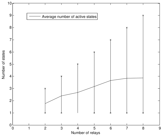
Figure 2: Average, minimum and maximum number of active states to characterize the capacity of a HD relay network.

The conjecture holds for the case of $2$ relays as proved in Theorem 4. We proceeded through the following numerical evaluations: for each value of $N\leq 8$, we generated uniformly at random the SNR exponents of the channel gains, we computed the entries of $\mathbf{A}$ in (12) with the Hungarian algorithm, we solved the LP in (12) with the simplex method and we counted the number of constraints that equal the optimal gDoF (which is a known upper bound on the number of non zero entries of an optimal solution). The minimum and the maximum number of active states were found to be $1$ and $N+1$, respectively, as shown in Fig. 2, which also shows the average number of active states computed by giving an equal weight to all the tried channels. Note that the minimum number of active states for a generic HD relay network with $N$ relays has to be at least $N+1$. To see this, consider a ‘line network’ where the source can only communicate with relay 1, relay 1 can only communicate with relay 2, etc, and relay $N$ can only communicate with the destination; in a line network, $N+1$ non-zero states are necessary to enable the source to communicate with the destination. It is interesting that the minimum number of active states given by $N+1$ also appears to be the required maximum number of active states for achieving the optimal gDoF-wise network operation. If the reduction of the number of active states from exponential to linear as conjectured holds, it offers a simpler and more amenable way to design the network [19].

V Fully-connected relay network with $N=2$ relays

To gain insights into how relays are best utilized, we consider a network with $N=2$ relays. The analysis presented here differs from the one in [19] in the following: (i) we study the fully-connected network, while in [19] only the diamond network is treated; (ii) we explicitly find under which channel conditions the gDoF performance is enhanced by exploiting both relays instead of using only the best one, and (iii) we provide insights into the nature of the rate gain in networks with multiple HD relays.

We consider the parameterization in (13) where, in order to increase the readability of the document, the SNR-exponents are indicated as

$$\left[\frac{\log(|h_{ij}|^{2})}{\log(\mathsf{SNR})}\right]_{(i,j)\in[1:3]^{2}}=\begin{pmatrix}\star&\beta_{1}&\alpha_{s1}\\ \beta_{2}&\star&\alpha_{s2}\\ \alpha_{1d}&\alpha_{2d}&1\\ \end{pmatrix},$$ (13)

where $\star$ denotes an entry that does not matter for channel capacity (because a relay can remove the ‘self-interference’), $\alpha_{si}$ is the SNR-exponent on the link from the source to relay $i$, $i\in[1:2]$, $\alpha_{id}$ is the SNR-exponent on the link from relay $i$, $i\in[1:2]$, to the destination, $\beta_{i}$ is the SNR-exponent on the link from relay $j$ to relay $i$, $(i,j)\in[1:2]^{2}$ with $j\not=i$, and the direct link from the source to the destination (entry in position (3,3) in (13)) has SNR-exponent normalized to 1 without loss of generality. Note that in order to consider a network without a direct link it suffices to consider all the other SNR-exponents to be larger than 1, or simply replace ‘1’ with ‘0’ in the discussion in the rest of the section.

We next derive the gDoF in both the FD and HD cases.

V-A The Full-Duplex Case

For the FD case, the cut-set bound is achievable to within $2\times 0.5105\times 4=4.084$ bits with NNC (see Remark 3). As a consequence, it can be verified that the gDoF for the FD case is

$$\mathsf{d}_{N=2}^{\rm(FD)}=\min\Big{\{} \max\left\{1,\alpha_{s1},\alpha_{s2}\right\},\max\left\{\alpha_{s2}+\alpha_{1d},\beta_{2}+1\right\},$$

$$\max\left\{\alpha_{s1}+\alpha_{2d},\beta_{1}+1\right\},\max\left\{1,\alpha_{1d},\alpha_{2d}\right\}\Big{\}}\geq 1.$$ (14)

Notice that the gDoF in (14) is no smaller than the gDoF that could be achieved by not using the relays, that is, by communicating directly through the direct link to achieve gDoF $=1$. Notice also that the gDoF in (14) does not change if we exchange $\alpha_{s1}$ with $\alpha_{2d}$ and $\alpha_{s2}$ with $\alpha_{1d}$, i.e., if we swap the role of the source and destination. We aim to identify the channel conditions under which using both relays strictly improves the gDoF compared to the best-relay selection policy (which includes direct transmission from the source to the destination as a special case) that achieves

$$\mathsf{d}_{N=2,\text{best relay}}^{\rm(FD)} =\max\big{\{}1,\min\{\alpha_{s1},\alpha_{1d}\},\min\{\alpha_{s2},\alpha_{2d}\}\big{\}}\in[1,\mathsf{d}_{N=2}^{\rm(FD)}].$$ (15)

We distinguish the following cases:

Case 1): if

$$\text{either}\ \left\{\begin{array}[]{l}\alpha_{s1}\geq\alpha_{s2}\\ \alpha_{1d}\geq\alpha_{2d}\\ \end{array}\right.\text{or}\ \left\{\begin{array}[]{l}\alpha_{s1}<\alpha_{s2}\\ \alpha_{1d}<\alpha_{2d}\\ \end{array}\right.$$

then, since one of the relays is ‘uniformly better’ than the other, we immediately see that $\mathsf{d}_{N=2}^{\rm(FD)}=\mathsf{d}_{N=2,\text{best relay}}^{\rm(FD)}$, so in this regime selecting the best relay for transmission is gDoF optimal.

Case 2): if not in Case 1, then we are in

$$\text{either}\ \left\{\begin{array}[]{l}\alpha_{s1}\geq\alpha_{s2}\\ \alpha_{1d}<\alpha_{2d}\\ \end{array}\right.\text{or}\ \left\{\begin{array}[]{l}\alpha_{s1}<\alpha_{s2}\\ \alpha_{1d}\geq\alpha_{2d}\\ \end{array}\right..$$

Consider the case $\alpha_{s2}\leq\alpha_{s1},\ \alpha_{1d}<\alpha_{2d}$ (the other one is obtained essentially by swapping the role of the relays). This corresponds to an ‘asymmetric’ situation where relay 1 has the best link from the source but relay 2 has the best link to the destination. In this case we would like to exploit the inter relay communication links (which is not present in a diamond network) to create a route source$\to$relay1$\to$relay2$\to$destination in addition to the direct link source$\to$destination. Indeed, in this case $\mathsf{d}_{N=2}^{\rm(FD)}$ in (14) can be rewritten as

$$\mathsf{d}_{N=2}^{\rm(FD)}=\min\Big{\{}\max\left\{\alpha_{s2}+\alpha_{1d},\beta_{2}+1\right\},\max\{1,\min\{\alpha_{s1},\alpha_{2d}\}\}\Big{\}},$$ (16)

where the term $\max\{1,\min\{\alpha_{s1},\alpha_{2d}\}\}$ in (16) corresponds to the gDoF of a virtual single-relay channel such that the link from the source to the “virtual relay” has SNR-exponent $\alpha_{s1}$ and the link from the “virtual relay” to the destination has SNR-exponent $\alpha_{2d}$. We aim to determine the subset of the channel parameters $\alpha_{s2}\leq\alpha_{s1},\ \alpha_{1d}<\alpha_{2d}$ for which the gDoF in (16) is strictly larger than the ‘best relay’ gDoF in (15). The case $\alpha_{s2}\leq\alpha_{s1},\ \alpha_{1d}<\alpha_{2d}$ subsumes the following possible orders of the channel gains:

$$\begin{array}[]{|l| l l l l l l l l |}\hline\cr\text{case i }&\alpha_{1d}&\alpha_{2d}&\alpha_{s2}&&&\alpha_{s1}&&\\ \hline\cr\text{case ii }&\alpha_{1d}&&\alpha_{s2}&\alpha_{2d}&&\alpha_{s1}&&\\ \hline\cr\text{case iii}&\alpha_{1d}&&\alpha_{s2}&&&\alpha_{s1}&\alpha_{2d}&\\ \hline\cr\text{case iv }&&&\alpha_{s2}&\alpha_{1d}&\alpha_{2d}&\alpha_{s1}&&\\ \hline\cr\text{case v }&&&\alpha_{s2}&\alpha_{1d}&&\alpha_{s1}&\alpha_{2d}&\\ \hline\cr\text{case vi }&&&\alpha_{s2}&&&\alpha_{s1}&\alpha_{1d}&\alpha_{2d}\\ \hline\cr\end{array}$$

We partition the set of channel parameters $\alpha_{s2}\leq\alpha_{s1},\ \alpha_{1d}<\alpha_{2d}$ as follows:

• Sub-case 2a) (all but cases i and vi in the table above): if

  $$\max\{\alpha_{s2},\alpha_{1d}\}<\min\{\alpha_{s1},\alpha_{2d}\},\ \$$ (17)

  then

  $$\mathsf{d}_{N=2,\text{best relay}}^{\rm(FD)}=\max\{1,\alpha_{s2},\alpha_{1d}\},$$ (18)

  which is strictly less than $\mathsf{d}_{N=2}^{\rm(FD)}$ in (16) if

  either $$\max\{1,\alpha_{s2},\alpha_{1d}\}<\min\{\alpha_{s1},\alpha_{2d}\}\leq\max\left\{\alpha_{s2}+\alpha_{1d},\beta_{2}+1\right\}$$

  or $$\Big{\{}\max\left\{\alpha_{s2}+\alpha_{1d},\beta_{2}+1\right\}<\min\{\alpha_{s1},\alpha_{2d}\}\Big{\}}\cap\mathcal{O}^{c}$$

  where $$\mathcal{O}\!:=\!\{\beta_{2}\!=\!0,\alpha_{s2}\!+\!\alpha_{1d}\!\leq\!1\}\cup\{\alpha_{1d}\!=\!0,\beta_{2}\!+\!1\!\leq\!\alpha_{s2}\}\cup\{\alpha_{s2}\!=\!0,\beta_{2}\!+\!1\!\leq\!\alpha_{1d}\}.$$

  that is, for

  $$\max\{1,\alpha_{s2},\alpha_{1d}\}<\min\{\alpha_{s1},\alpha_{2d}\}\ \text{except in region $\mathcal{O}$}.$$ (19)

• Sub-case 2b) (case i in the table above): if $\alpha_{1d}<\alpha_{2d}\leq\alpha_{s2}\leq\alpha_{s1}$, then the condition

  $$\mathsf{d}_{N=2,\text{best relay}}^{\rm(FD)}=\max\{1,\alpha_{2d}\}<\mathsf{d}_{N=2}^{\rm(FD)}=\min\Big{\{}\max\left\{\alpha_{s2}+\alpha_{1d},\beta_{2}+1\right\},\max\{1,\alpha_{2d}\}\Big{\}}$$

  is never verified, i.e., in this case $\mathsf{d}_{N=2,\text{best relay}}^{\rm(FD)}=\mathsf{d}_{N=2}^{\rm(FD)}$.

• Sub-case 2c) (case vi in the table above): if $\alpha_{s2}\leq\alpha_{s1}\leq\alpha_{1d}<\alpha_{2d}$, then

  $$\mathsf{d}_{N=2,\text{best relay}}^{\rm(FD)}=\max\{1,\alpha_{s1}\}<\mathsf{d}_{N=2}^{\rm(FD)}=\min\Big{\{}\max\left\{\alpha_{s2}+\alpha_{1d},\beta_{2}+1\right\},\max\{1,\alpha_{s1}\}\Big{\}}$$

  is never verified, i.e., in this case $\mathsf{d}_{N=2,\text{best relay}}^{\rm(FD)}=\mathsf{d}_{N=2}^{\rm(FD)}$.

Recall that there is also a regime similar Case 2) where the role of the relays is swapped.

Fig. 3 gives an example of a network satisfying the conditions in (17), i.e., the assumption is $0\leq y<x$ without loss of generality. By exploiting both relays, the system attains

$$\mathsf{d}_{N=2}^{\rm(FD)} =\min\Big{\{}\max\{1,x,y\},\max\{2x,z+1\},\max\{2y,z+1\}\Big{\}}$$

$$=\min\Big{\{}\max\{1,x\},\max\{2y,z+1\}\Big{\}},$$

while, by using only the best relay, it achieves

$$\mathsf{d}_{N=2,\text{best relay}}^{\rm(FD)} =\max\big{\{}1,\min\{x,y\}\big{\}}=\max\big{\{}1,y\big{\}}.$$

By (19), we have $\mathsf{d}_{N=2}^{\rm(FD)}>\mathsf{d}_{N=2,\text{best relay}}^{\rm(FD)}$ if

$$x>\max\big{\{}1,y\big{\}}\ \text{except}\ \left\{z=0,y\leq\frac{1}{2}\right\}.$$ (20)

V-B The Half-Duplex Case

With HD, the gDoF is given by (12), which with the notation in (13) and with $\lambda_{1}=\lambda_{00}$, $\lambda_{2}=\lambda_{01}$, $\lambda_{3}=\lambda_{10}$ and $\lambda_{4}=\lambda_{11}$ becomes

$$\mathsf{d}_{N=2}^{\rm(HD)}=\max\min\Big{\{} \lambda_{00}D_{1}^{(0)}+\lambda_{01}D_{1}^{(1)}+\lambda_{10}D_{1}^{(2)}+\lambda_{11}D_{1}^{(3)},$$

$$\lambda_{00}D_{2}^{(0)}+\lambda_{01}D_{2}^{(1)}+\lambda_{10}D_{2}^{(2)}+\lambda_{11}D_{2}^{(3)},$$

$$\lambda_{00}D_{3}^{(0)}+\lambda_{01}D_{3}^{(1)}+\lambda_{10}D_{3}^{(2)}+\lambda_{11}D_{3}^{(3)},$$

$$\lambda_{00}D_{4}^{(0)}+\lambda_{01}D_{4}^{(1)}+\lambda_{10}D_{4}^{(2)}+\lambda_{11}D_{4}^{(3)}\Big{\}},$$ (21)

where the maximization is over $\lambda_{ij}=\mathbb{P}[S_{1}=i,S_{2}=j]\geq 0$, $(i,j)\in\{0,1\}^{2}$, such that $\lambda_{00}+\lambda_{01}+\lambda_{10}+\lambda_{11}=1$ and

$$\begin{array}[]{ll}D_{1}^{(0)}:=\max\left\{1,\alpha_{s1},\alpha_{s2}\right\},&D_{1}^{(1)}=D_{2}^{(0)}:=\max\left\{1,\alpha_{s1}\right\},\\ D_{4}^{(3)}:=\max\left\{1,\alpha_{1d},\alpha_{2d}\right\},&D_{1}^{(2)}=D_{3}^{(0)}:=\max\left\{1,\alpha_{s2}\right\},\\ D_{2}^{(1)}:=\max\left\{\alpha_{s1}+\alpha_{2d},\beta_{1}+1\right\},&D_{2}^{(3)}=D_{4}^{(1)}:=\max\left\{1,\alpha_{2d}\right\},\\ D_{3}^{(2)}:=\max\left\{\alpha_{s2}+\alpha_{1d},\beta_{2}+1\right\},&D_{3}^{(3)}=D_{4}^{(2)}:=\max\left\{1,\alpha_{1d}\right\},\\ D_{1}^{(3)}=D_{2}^{(2)}=D_{3}^{(1)}=D_{4}^{(0)}:=1.\end{array}$$

For future reference, if only one relay helps the communication between the source and the destination then the achievable gDoF is [25]

$$\mathsf{d}_{N=2,\text{best relay}}^{\rm(HD)} =1+\max_{i\in[1:2]}\frac{[\alpha_{si}-1]^{+}\ [\alpha_{id}-1]^{+}}{[\alpha_{si}-1]^{+}+[\alpha_{id}-1]^{+}}\in[1,\mathsf{d}_{N=2}^{\rm(HD)}].$$ (22)

An analytical closed form solution for the optimal $\{\lambda_{ij}\}$ in (21) is complex to find for general channel gain assignments. However, numerically it is a question of solving a LP, for which efficient numerical routines exist. By using Theorem 4, we can set either $\lambda_{00}$ or $\lambda_{11}$ to zero.

For the example in Fig. 3 the optimal schedule has $\lambda_{00}=\lambda_{11}=0$ without loss of optimality, from Theorem 4. By letting $\lambda_{01}=\gamma\in[0,1]$ and $\lambda_{10}=1-\gamma$ (recall $0\leq y<x$ without loss of generality), the gDoF in (21) can be written as

$$\mathsf{d}_{N=2}^{\rm(HD)}=\max_{\gamma\in[0,1]}\min\Big{\{} \gamma\max\{1,x\}+(1-\gamma)\max\{1,y\},$$ (23a)

$$\gamma\max\{2x,z+1\}+(1-\gamma),$$ (23b)

$$\gamma+(1-\gamma)\max\{2y,z+1\}\Big{\}}$$ (23c)

$$=1+\min \left\{\frac{[x-1]^{+}\max\{2y-1,z\}}{[x-1]^{+}+\max\{2y-1,z\}-[y-1]^{+}},\right.$$ (23d)

$$\left.\frac{\max\{2x-1,z\}\max\{2y-1,z\}}{\max\{2x-1,z\}+\max\{2y-1,z\}}\right\}.$$ (23e)

By using only the best relay as in (22), we would achieve

$$\mathsf{d}_{N=2,\text{best relay}}^{\rm(HD)} =1+\frac{[x-1]^{+}[y-1]^{+}}{[x-1]^{+}+[y-1]^{+}}.$$ (24)

It can be easily seen that the best relay selection policy is strictly suboptimal if (20) is verified, as for the FD case.

VI Conclusions

In this work we analyzed a network where a source communicates with a destination across a Gaussian channel. This communication is assisted by $N$ relays operating in half-duplex mode. We characterized the capacity to within a constant gap by using an achievable scheme based on noisy network coding. We also showed that this gap may be further reduced by considering more structured systems, such as the diamond network. We conjectured that the optimal schedule has at most $N+1$ active states, instead of the possible $2^{N}$. This conjecture has been supported by the analytical proof in the special case of $N=2$ relays and in general by numerical evaluations. We finally analyzed a network with $N=2$ relays, and we showed under which channel conditions by exploiting both relays a strictly greater gDoF can be attained compared to a network where best-relay selection is used.

An interesting connection between the high-SNR approximation of the point-to-point MIMO capacity and the Maximum Weighted Bipartite Matching problem from graph theory has been discovered.

Appendix A Proof of Proposition 1

In a multicast network, where $\mathbf{H}_{\rm r\to r}=0$ and $\mathbf{H}_{\rm s\to d}=0$ in (2), the rank of any channel sub matrix is upper bounded by $2$. Thus, with ${\rm Rank}[\mathbf{H}_{\mathcal{A},s}]\leq 2$ in the cut-set bound in the step preceding (7) and by using the NNC lower bound in (6), the gap becomes

$$\mathsf{GAP} \leq\min_{\gamma\geq\mathrm{e}-1}\max_{\mu\in[0:1]}\left\{2\min\left\{\frac{\gamma}{\mathrm{e}},\frac{2}{\mu K}\right\}\log\left(\max\left\{\mathrm{e},\frac{\gamma\ \mu K}{2}\right\}\right)\right.\left.+\mu K\log\left(\frac{2\gamma}{\gamma-1}\right)\right\}$$

$$\stackrel{{\scriptstyle(a)}}{{=}}\min_{\gamma\geq\mathrm{e}-1}\left.\left\{2\min\left\{\frac{\gamma}{\mathrm{e}},\frac{2}{K}\right\}\log\left(\mathrm{e}\max\left\{1,\frac{\gamma}{\mathrm{e}}\frac{K}{2}\right\}\right)\right.\right.\left.+K\log\left(\frac{2\gamma}{\gamma-1}\right)\right\}$$

$$\stackrel{{\scriptstyle(b)}}{{=}}\left\{\begin{array}[]{ll}2\log(\mathrm{e})\frac{1+\sqrt{1+2K\mathrm{e}}}{2\mathrm{e}}+K\log\left(\frac{2\sqrt{1+2K\mathrm{e}}+2}{\sqrt{1+2K\mathrm{e}}-1}\right)&\text{if}\ K\leq 2\\ \frac{4}{K}\log\left(\frac{K}{2}+\frac{K^{3}}{8}\right)+K\log\left(2+\frac{8}{K^{2}}\right)&\text{if}\ K>2\end{array},\right.$$

where: the equality in (a) follows since the function is always increasing in $\mu$ so the maximum is attained for $\mu^{\rm{opt}}=1$; the minimum over $\gamma$ is attained for

$$\gamma^{\rm opt}=\left\{\begin{array}[]{ll}\frac{1+\sqrt{1+2K\mathrm{e}}}{2}&\text{if}\ K\leq 2\\ 1+\frac{K^{2}}{4}&\text{if}\ K>2\end{array}\right.$$

and this leads to the equality in (b).

By substituting $K=N+2$ in order to obtain the special case of the HD multi-relay diamond network we get (9).

Appendix B Proof of Theorem 2

Let $\mathcal{S}_{n,k}$ be the set of all $k$-combinations of the integers in $[1:n]$ and $\mathcal{P}_{n,k}$ be the set of all $k$-permutations of the integers in $[1:n]$. Let $\sigma(\pi)$ be the sign / signature of the permutation $\pi$.

We start by demonstrating that the asymptotic behavior of $|\mathbf{I}_{k}+\mathbf{H}\mathbf{H}^{H}|$ is as that of $|\mathbf{H}\mathbf{H}^{H}|$, i.e., the identity matrix can be neglected. By using the determinant Leibniz formula [30], in fact we have,

$$|\mathbf{I}_{k}+\mathbf{H}\mathbf{H}^{H}|=\sum_{\pi\in\mathcal{P}_{n,k}}\sigma(\pi)\prod_{i=1}^{k}\left[\mathbf{I}_{k}+\mathbf{H}\mathbf{H}^{H}\right]_{i,\pi(i)}$$

$$=\sum_{\pi\in\mathcal{P}_{n,k}}\sigma(\pi)\left\{\left(\prod_{i=2}^{k}\left[\mathbf{I}_{k}+\mathbf{H}\mathbf{H}^{H}\right]_{i,\pi(i)}\right)\left(\left[\mathbf{I}_{k}+\mathbf{H}\mathbf{H}^{H}\right]_{1,\pi(1)}\right)\right\}$$

$$=\sum_{\pi\in\mathcal{P}_{n,k}}\sigma(\pi)\left(\prod_{i=2}^{k}\left[\mathbf{I}_{k}+\mathbf{H}\mathbf{H}^{H}\right]_{i,\pi(i)}\right)\delta[1-\pi(1)]$$

$$+\sum_{\pi\in\mathcal{P}_{n,k}}\sigma(\pi)\prod_{i=2}^{k}\left[\mathbf{I}_{k}+\mathbf{H}\mathbf{H}^{H}\right]_{i,\pi(i)}\left[\mathbf{H}\mathbf{H}^{H}\right]_{1,\pi(1)},$$

where $\delta[n]=\left\{\begin{array}[]{ll}0&n\neq 0\\ 1&n=0\end{array}\right.$ is the Kronecker delta. Let

$$\mathsf{A}\left(\mathsf{SNR}\right):=\sum_{\pi\in\mathcal{P}_{n,k}}\sigma(\pi)\left(\prod_{i=2}^{k}\left[\mathbf{I}_{k}+\mathbf{H}\mathbf{H}^{H}\right]_{i,\pi(i)}\right)\delta[1-\pi(1)]$$

$$\mathsf{B}\left(\mathsf{SNR}\right):=\sum_{\pi\in\mathcal{P}_{n,k}}\sigma(\pi)\prod_{i=2}^{k}\left[\mathbf{I}_{k}+\mathbf{H}\mathbf{H}^{H}\right]_{i,\pi(i)}\left[\mathbf{H}\mathbf{H}^{H}\right]_{1,\pi(1)},$$

we have that $\mathsf{A}\left(\mathsf{SNR}\right)=o\left(\mathsf{B}\left(\mathsf{SNR}\right)\right),\ \text{because}\ \lim\limits_{\mathsf{SNR}\to+\infty}\frac{\mathsf{A}\left(\mathsf{SNR}\right)}{\mathsf{B}\left(\mathsf{SNR}\right)}=0$ where the $\mathsf{SNR}$ parameterizes the channel gains as $|h_{ij}|^{2}=\mathsf{SNR}^{\beta_{ij}}$, for some non-negative $\beta_{ij}$. This is so because, as a function of $\mathsf{SNR}$, $\mathsf{B}\left(\mathsf{SNR}\right)$ grows faster than $\mathsf{A}\left(\mathsf{SNR}\right)$ due to the term $\left[\mathbf{H}\mathbf{H}^{H}\right]_{1,\pi(1)}$. By induction it is possible to show that this reasoning holds $\forall i\in[1:k]$ and hence

$$|\mathbf{I}_{k}+\mathbf{H}\mathbf{H}^{H}|\doteq\sum_{\pi\in\mathcal{P}_{n,k}}\sigma(\pi)\prod_{i=1}^{k}\left[\mathbf{H}\mathbf{H}^{H}\right]_{i,\pi(i)}=|\mathbf{H}\mathbf{H}^{H}|.$$

Therefore, now we focus on the study of $|\mathbf{H}\mathbf{H}^{H}|$. We have

$$|\mathbf{H}\mathbf{H}^{H}|\stackrel{{\scriptstyle(a)}}{{=}}\sum_{\varsigma\in\mathcal{S}_{n,k}}|\mathbf{H}_{\varsigma}||\mathbf{H}_{\varsigma}^{H}|=\sum_{\varsigma\in\mathcal{S}_{n,k}}|\mathbf{H}_{\varsigma}|^{2}$$

$$\stackrel{{\scriptstyle(b)}}{{=}}\sum_{\varsigma\in\mathcal{S}_{n,k}}\left|\sum_{\pi\in\mathcal{P}_{n,k}}\sigma(\pi)\prod_{i=1}^{k}\left[\mathbf{H}_{\varsigma}\right]_{i,\pi(i)}\right|^{2}$$

$$=\sum_{\varsigma\in\mathcal{S}_{n,k}}\left\{\left(\sum_{\pi_{1}\in\mathcal{P}_{n,k}}\sigma(\pi_{1})\prod_{i=1}^{k}\left[\mathbf{H}_{\varsigma}\right]_{i,{\pi_{1}}(i)}\right)\left(\sum_{\pi_{2}\in\mathcal{P}_{n,k}}\sigma(\pi_{2})\prod_{j=1}^{k}\left[\mathbf{H}_{\varsigma}\right]_{j,{\pi_{2}}(j)}\right)^{*}\right\}$$

$$=\sum_{\varsigma\in\mathcal{S}_{n,k}}\left\{\left(\sum_{\pi\in\mathcal{P}_{n,k}}\prod_{i=1}^{k}\left|\left[\mathbf{H}_{\varsigma}\right]_{i,{\pi}(i)}\right|^{2}\right)\right.$$

$$\left.+\left(\sum_{\pi_{1},\pi_{2}\in\mathcal{P}_{n,k},\pi_{1}\neq\pi_{2}}\sigma(\pi_{1})\sigma(\pi_{2})\prod_{i=1}^{k}\prod_{j=1}^{k}\left[\mathbf{H}_{\varsigma}\right]_{i,{{\pi}_{1}}(i)}\left(\left[\mathbf{H}_{\varsigma}\right]_{j,{{\pi}_{2}}(j)}\right)^{*}\right)\right\}$$

$$\stackrel{{\scriptstyle(c)}}{{\leq}}\sum_{\varsigma\in\mathcal{S}_{n,k}}\left\{\left(\sum_{\pi\in\mathcal{P}_{n,k}}\prod_{i=1}^{k}\left|\left[\mathbf{H}_{\varsigma}\right]_{i,{\pi}(i)}\right|^{2}\right)\right.$$

$$\left.+\left(\sum_{\pi_{1},\pi_{2}\in\mathcal{P}_{n,k},\pi_{1}\neq\pi_{2}}\prod_{i=1}^{k}\prod_{j=1}^{k}\sqrt{\left|\left[\mathbf{H}_{\varsigma}\right]_{i,{{\pi}_{1}}(i)}\right|^{2}\left|\left[\mathbf{H}_{\varsigma}\right]_{j,{{\pi}_{2}}(j)}\right|^{2}}\right)\right\}$$

$$=\sum_{\varsigma\in\mathcal{S}_{n,k}}\left\{\left(\sum_{\pi\in\mathcal{P}_{n,k}}\mathsf{SNR}^{\sum_{i=1}^{k}\left[\mathbf{B}_{\varsigma}\right]_{i,\pi(i)}}\right)\right.$$

$$\left.+\left(\sum_{\pi_{1},\pi_{2}\in\mathcal{P}_{n,k},\pi_{1}\neq\pi_{2}}\mathsf{SNR}^{\frac{1}{2}\left(\sum_{i=1}^{k}\left[\mathbf{B}_{\varsigma}\right]_{i,{\pi_{1}}(i)}+\sum_{j=1}^{k}\left[\mathbf{B}_{\varsigma}\right]_{j,{\pi_{2}}(j)}\right)}\right)\right\}$$

$$\stackrel{{\scriptstyle(d)}}{{\doteq}}\sum_{\varsigma\in\mathcal{S}_{n,k}}\left(\sum_{\pi\in\mathcal{P}_{n,k}}\mathsf{SNR}^{\sum_{i=1}^{k}\left[\mathbf{B}_{\varsigma}\right]_{i,\pi(i)}}\right)$$

$${\doteq}\ \mathsf{SNR}^{\max_{\varsigma\in\mathcal{S}_{n,k}}\max_{\pi\in\mathcal{P}_{n,k}}\sum_{i=1}^{k}\left[\mathbf{B}_{\varsigma}\right]_{i,\pi(i)}},$$

where the equalities / inequalities above are due to the following facts:

• equality (a): by applying the Cauchy-Binet formula [30] where $\mathbf{H}_{\varsigma}$ is the square matrix obtained from $\mathbf{H}$ by retaining all rows and those columns indexed by $\varsigma$;

• equality (b): by applying the determinant Leibniz formula [30];

• inequality (c): by applying the Cauchy-Swartz inequality [31];

• equality (d): when $\mathsf{SNR}\rightarrow\infty$, we have

  $$\sum_{i=1}^{k}\left[\mathbf{B}_{\varsigma}\right]_{i,\pi(i)}\geq\frac{1}{2}\left(\sum_{i=1}^{k}\left[\mathbf{B}_{\varsigma}\right]_{i,{\pi_{1}}(i)}+\sum_{j=1}^{k}\left[\mathbf{B}_{\varsigma}\right]_{j,{\pi_{2}}(j)}\right).$$

  Consider the following example. Let $a=\mathsf{SNR}^{\beta_{a}}$, $b=\mathsf{SNR}^{\beta_{b}}$, $c=\mathsf{SNR}^{\beta_{c}}$, $d=\mathsf{SNR}^{\beta_{d}}$

  $$|ab-cd|^{2}\leq|a|^{2}|b|^{2}+|c|^{2}|d|^{2}+2|a||b||c||d|.$$

  Now apply the gDoF formula, i.e.,

  $$\mathsf{d} :=\lim\limits_{\mathsf{SNR}\to+\infty}\frac{\log\left(|a|^{2}|b|^{2}+|c|^{2}|d|^{2}+2|a||b||c||d|\right)}{\log(1+\mathsf{SNR})}$$

  $$=\max\left\{\beta_{a}+\beta_{b},\beta_{c}+\beta_{d},\frac{\beta_{a}+\beta_{b}+\beta_{c}+\beta_{d}}{2}\right\},$$

  but

  $$\frac{\beta_{a}+\beta_{b}+\beta_{c}+\beta_{d}}{2}\leq\frac{2\max\left\{\beta_{a}+\beta_{b},\beta_{c}+\beta_{d}\right\}}{2}=\max\left\{\beta_{a}+\beta_{b},\beta_{c}+\beta_{d}\right\}.$$

  Therefore, the term $\frac{\beta_{a}+\beta_{b}+\beta_{c}+\beta_{d}}{2}$ does not contribute in characterizing the gDoF. By direct induction, the above reasoning may be extended to a general number of terms leading to $\sum_{i=1}^{k}\left[\mathbf{B}_{\varsigma}\right]_{i,\pi(i)}\geq\frac{1}{2}\left(\sum_{i=1}^{k}\left[\mathbf{B}_{\varsigma}\right]_{i,{\pi_{1}}(i)}+\sum_{j=1}^{k}\left[\mathbf{B}_{\varsigma}\right]_{j,{\pi_{2}}(j)}\right)$.

Appendix C Proof of Theorem 4

In a HD relay network with $N=2$, we have $4$ possible states that may arise with probabilities $\lambda_{j}$ with $j\in[1,4]$. We let $\lambda_{1}=\lambda_{00}$, $\lambda_{2}=\lambda_{01}$, $\lambda_{3}=\lambda_{10}$ and $\lambda_{4}=\lambda_{11}$, where $\lambda_{ij}=\mathbb{P}[S_{1}=i,S_{2}=j]\geq 0$, $(i,j)\in\{0,1\}^{2}$, such that $\lambda_{00}+\lambda_{01}+\lambda_{10}+\lambda_{11}=1$. Here we aim to demonstrate that a schedule with $\lambda_{00}\lambda_{11}=0$ is optimal, i.e., it maximizes the capacity of the HD relay network with $N=2$. Let

$$\alpha_{s1}-1:=\alpha^{\star}_{s1},\quad\alpha_{s2}-1:=\alpha^{\star}_{s2},$$

$$\alpha_{1d}-1:=\alpha^{\star}_{1d},\quad\alpha_{2d}-1:=\alpha^{\star}_{2d}.$$

The LP in (12) with the notation in (13) becomes

$$\mathsf{d}_{N=2}^{\rm(HD)}=1+\max\min\Big{\{} \lambda_{00}D_{1}^{(0)}+\lambda_{01}D_{1}^{(1)}+\lambda_{10}D_{1}^{(2)}+\lambda_{11}D_{1}^{(3)},$$

$$\lambda_{00}D_{2}^{(0)}+\lambda_{01}D_{2}^{(1)}+\lambda_{10}D_{2}^{(2)}+\lambda_{11}D_{2}^{(3)},$$

$$\lambda_{00}D_{3}^{(0)}+\lambda_{01}D_{3}^{(1)}+\lambda_{10}D_{3}^{(2)}+\lambda_{11}D_{3}^{(3)},$$

$$\lambda_{00}D_{4}^{(0)}+\lambda_{01}D_{4}^{(1)}+\lambda_{10}D_{4}^{(2)}+\lambda_{11}D_{4}^{(3)}\Big{\}},$$ (25)

where

$$\begin{array}[]{ll}D_{1}^{(0)}:=\max\left\{0,\alpha^{\star}_{s1},\alpha^{\star}_{s2}\right\},&D_{1}^{(1)}=D_{2}^{(0)}:=\max\left\{0,\alpha^{\star}_{s1}\right\},\\ D_{4}^{(3)}:=\max\left\{0,\alpha^{\star}_{1d},\alpha^{\star}_{2d}\right\},&D_{1}^{(2)}=D_{3}^{(0)}:=\max\left\{0,\alpha^{\star}_{s2}\right\},\\ D_{2}^{(1)}:=\max\left\{\alpha^{\star}_{s1}+\alpha^{\star}_{2d}+1,\beta_{1}\right\},&D_{2}^{(3)}=D_{4}^{(1)}:=\max\left\{0,\alpha_{2d}\right\},\\ D_{3}^{(2)}:=\max\left\{\alpha^{\star}_{s2}+\alpha^{\star}_{1d}+1,\beta_{2}\right\},&D_{3}^{(3)}=D_{4}^{(2)}:=\max\left\{0,\alpha^{\star}_{1d}\right\},\\ D_{1}^{(3)}=D_{2}^{(2)}=D_{3}^{(1)}=D_{4}^{(0)}:=0.\end{array}$$

Now we have to consider the different cases that may arise:

• Case 1: $\max\left\{0,\alpha^{\star}_{s1},\alpha^{\star}_{s2}\right\}=0\Longleftrightarrow\alpha^{\star}_{s1}\leq 0,\alpha^{\star}_{s2}\leq 0$. In this case we have:

  $$D_{1}^{(0)}=D_{2}^{(0)}=D_{3}^{(0)}=D_{4}^{(0)}=0,$$

  that is $\lambda_{00}$ is not involved in the optimization; hence, we can set $\lambda_{00}=0$ without loss of optimality.

• Case 2 a: $\alpha^{\star}_{s1}>0,\alpha^{\star}_{s2}\leq 0$. In this case we have

  $$\mathsf{d}=1+\max_{(\lambda_{00},\lambda_{01},\lambda_{10},\lambda_{11})\in[0,1]^{4}:\lambda_{00}+\lambda_{10}+\lambda_{01}+\lambda_{11}\leq 1}\min\left\{\right.$$

  $$\left.\begin{array}[]{llll}\lambda_{00}\alpha^{\star}_{s1}&+\lambda_{01}\alpha^{\star}_{s1}&+0&+0\\ 0&+0&+\lambda_{10}\max\left\{\alpha^{\star}_{s2}+\alpha^{\star}_{1d}+1,\beta_{2}\right\}&+\lambda_{11}\max\left\{0,\alpha^{\star}_{1d}\right\}\\ 0&+\lambda_{01}\max\left\{0,\alpha^{\star}_{2d}\right\}&+\lambda_{10}\max\left\{0,\alpha^{\star}_{1d}\right\}&+\lambda_{11}\max\left\{0,\alpha^{\star}_{1d},\alpha^{\star}_{2d}\right\}\\ \end{array}\right\},$$

  since the second constraint in (25) is always greater than the first one.

  Assume $(\lambda_{00},\lambda_{01},\lambda_{10},\lambda_{11})$ is optimal with $\lambda_{00}>0$; the solution $(0,\lambda_{00}+\lambda_{01},\lambda_{10},\lambda_{11})$ gives a higher gDoF (the first and the second equations remain the same, the last one is increased); we reached a contradiction. Hence the optimal solution must have $\lambda_{00}=0$.

• Case 2 b: $\alpha^{\star}_{s1}\leq 0,\alpha^{\star}_{s2}>0$. As Case 2 a above but with the role of the sources swapped. Also in this case the optimal solution must have $\lambda_{00}=0$.

• So far we showed that if $\min\left\{\alpha^{\star}_{s1},\alpha^{\star}_{s2}\right\}\leq 0$ then $\lambda_{00}=0$ is optimal. Due to the symmetry of the problem, by swapping $\alpha^{\star}_{sj}$ with $\alpha^{\star}_{jd}$, if $\min\left\{\alpha^{\star}_{1d},\alpha^{\star}_{2d}\right\}\leq 0$, then $\lambda_{11}=0$ is optimal.

  In oder to prove our claim we must consider one last case:

  $$\min\left\{\alpha^{\star}_{s1},\alpha^{\star}_{s2}\right\}>0\ \text{and}\ \min\left\{\alpha^{\star}_{1d},\alpha^{\star}_{2d}\right\}>0,$$ (26)

  that is when all the links from the source to the relays and all links from the relays to the destination are strictly larger than the direct link.

  In order to prove our claim, we must partition the set of parameters in (26) into two regimes, say $O_{0}$ and $O_{1}$, where in regime $O_{0}$ we show $\lambda_{00}=0$ is optimal and in regime $O_{1}$ that $\lambda_{11}=0$ is optimal. By the symmetry of the problem when swapping $\alpha^{\star}_{sj}$ with $\alpha^{\star}_{jd}$, the regime $O_{0}$ must be equal to regime $O_{1}$ when $\alpha^{\star}_{sj}$ and $\alpha^{\star}_{jd}$ are swapped. Next we show that

  $$O_{0}=\{\alpha^{\star}_{s1}\alpha^{\star}_{s2}\geq\alpha^{\star}_{1d}\alpha^{\star}_{2d}\},\ O_{1}=\{\alpha^{\star}_{s1}\alpha^{\star}_{s2}\leq\alpha^{\star}_{1d}\alpha^{\star}_{2d}\}.$$

• Case 3: $\alpha^{\star}_{s1}>0,\alpha^{\star}_{s2}>0,\alpha^{\star}_{1d}>0,\alpha^{\star}_{2d}>0$. Without loss of generality, we assume $\alpha_{1d}\geq\alpha_{2d}$; in this case we have

  $$\begin{array}[]{ll}D_{1}^{(0)}:=\max\left\{\alpha^{\star}_{s1},\alpha^{\star}_{s2}\right\},&D_{1}^{(1)}=D_{2}^{(0)}:=\alpha^{\star}_{s1},\\ D_{1}^{(2)}=D_{3}^{(0)}:=\alpha^{\star}_{s2},&D_{1}^{(3)}=D_{2}^{(2)}=D_{3}^{(1)}=D_{4}^{(0)}:=0,\\ D_{2}^{(1)}:=\max\left\{\alpha^{\star}_{s1}+\alpha^{\star}_{2d}+1,\beta_{1}\right\},&D_{2}^{(3)}=D_{4}^{(1)}:=\alpha^{\star}_{2d},\\ D_{3}^{(2)}:=\max\left\{\alpha^{\star}_{s2}+\alpha^{\star}_{1d}+1,\beta_{2}\right\},&D_{3}^{(3)}=D_{4}^{(2)}=D_{4}^{(3)}:=\alpha^{\star}_{1d}.\end{array}$$

  Now we aim to find the conditions under which setting $\lambda_{00}=0$ increases the gDoF compared to a case where $\lambda_{00}>0$. Finding these conditions is equivalent to solve a system where $\lambda_{00}$ is now split into three parts, that we name $\lambda^{\star}_{01}$, $\lambda^{\star}_{10}$ and $\lambda^{\star}_{11}$. In other words, our aim is to demonstrate that $\left(0,\lambda_{01}+\lambda^{\star}_{01},\lambda_{10}+\lambda^{\star}_{10},\lambda_{11}+\lambda^{\star}_{11}\right)$ gives a larger gDoF than $\left(\lambda_{00},\lambda_{01},\lambda_{10},\lambda_{11}\right)$ with $\lambda_{00}=\lambda^{\star}_{01}+\lambda^{\star}_{10}+\lambda^{\star}_{11}$. This is equivalent to solve

  $$x\max\left\{\alpha^{\star}_{s1},\alpha^{\star}_{s2}\right\}\leq\lambda^{\star}_{01}\alpha^{\star}_{s1}+\lambda^{\star}_{10}\alpha^{\star}_{s2}$$

  $$x\alpha^{\star}_{s2}\leq\lambda^{\star}_{10}\max\left\{\alpha^{\star}_{s2}+\alpha^{\star}_{1d}+1,\beta_{2}\right\}+\lambda^{\star}_{11}\alpha^{\star}_{1d}$$

  $$x\alpha^{\star}_{s1}\leq\lambda^{\star}_{01}\max\left\{\alpha^{\star}_{s1}+\alpha^{\star}_{2d}+1,\beta_{1}\right\}+\lambda^{\star}_{11}\alpha^{\star}_{2d}$$

  $$0\leq\lambda^{\star}_{01}\alpha^{\star}_{2d}+\lambda^{\star}_{10}\alpha^{\star}_{1d}+\lambda^{\star}_{11}\alpha^{\star}_{1d},$$

  where $\lambda^{\star}_{01}+\lambda^{\star}_{10}+\lambda^{\star}_{11}=x$. Now, by substituting $\lambda^{\star}_{11}=x-\lambda^{\star}_{01}-\lambda^{\star}_{10}$, we obtain

  $$x\max\left\{\alpha^{\star}_{s1},\alpha^{\star}_{s2}\right\}\leq\lambda^{\star}_{01}\alpha^{\star}_{s1}+\lambda^{\star}_{10}\alpha^{\star}_{s2}$$

  $$x\left(\alpha^{\star}_{s2}-\alpha^{\star}_{1d}\right)\leq\lambda^{\star}_{10}\max\left\{\alpha^{\star}_{s2}+1,\beta_{2}-\alpha^{\star}_{1d}\right\}-\lambda^{\star}_{01}\alpha^{\star}_{1d}$$

  $$x\left(\alpha^{\star}_{s1}-\alpha^{\star}_{2d}\right)\leq\lambda^{\star}_{01}\max\left\{\alpha^{\star}_{s1}+1,\beta_{1}-\alpha^{\star}_{2d}\right\}-\lambda^{\star}_{10}\alpha^{\star}_{2d}$$

  $$\lambda^{\star}_{01}\leq\frac{x\alpha^{\star}_{1d}}{\alpha^{\star}_{1d}-\alpha^{\star}_{2d}}.$$

  Notice that, in the last inequality, $\lambda^{\star}_{01}\leq 1$ holds if there exists a $0\leq x\leq 1$ such that $x\leq\frac{\alpha_{1d}-\alpha_{2d}}{\alpha_{1d}}$ and this is always true since $\frac{\alpha_{1d}-\alpha_{2d}}{\alpha_{1d}}\leq 1$. Assume equality in the last constraint and substitute the value of $\lambda^{\star}_{01}$ in the other inequalities. We obtain

  $$\lambda^{\star}_{10}\geq x\frac{\max\left\{\alpha^{\star}_{s1},\alpha^{\star}_{s2}\right\}\alpha^{\star}_{1d}-\max\left\{\alpha^{\star}_{s1},\alpha^{\star}_{s2}\right\}\alpha^{\star}_{2d}-\alpha^{\star}_{s1}\alpha^{\star}_{1d}}{\alpha^{\star}_{s2}\alpha^{\star}_{1d}-\alpha^{\star}_{s2}\alpha^{\star}_{2d}}:=\mathsf{A}$$ (27)

  $$\lambda^{\star}_{10}\geq x\frac{\alpha^{\star}_{s2}\alpha^{\star}_{1d}-\alpha^{\star}_{s2}\alpha^{\star}_{2d}+\alpha^{\star}_{1d}\alpha^{\star}_{2d}}{\max\left\{\alpha^{\star}_{s2}+1,\beta_{2}-\alpha^{\star}_{1d}\right\}\alpha^{\star}_{1d}-\max\left\{\alpha^{\star}_{s2}+1,\beta_{2}-\alpha^{\star}_{1d}\right\}\alpha^{\star}_{2d}}:=\mathsf{B}$$ (28)

  $$\lambda^{\star}_{10}\leq x\frac{\max\left\{\alpha^{\star}_{2d}+1,\beta_{1}-\alpha^{\star}_{s1}\right\}\alpha^{\star}_{1d}+\alpha^{\star}_{s1}{\alpha^{\star}_{2d}-\alpha^{\star}_{2d}}^{2}}{\alpha^{\star}_{1d}\alpha^{\star}_{2d}-{\alpha^{\star}_{2d}}^{2}}:=\mathsf{C}$$ (29)

  $$\lambda^{\star}_{01}=\frac{x\alpha^{\star}_{1d}}{\alpha^{\star}_{1d}-\alpha^{\star}_{2d}}.$$ (30)

  Thus we should have

  $$\max\left\{\mathsf{A},\mathsf{B}\right\}\leq\lambda^{\star}_{10},\quad\lambda^{\star}_{10}\leq\mathsf{C}$$

  which is possible if $\max\left\{\mathsf{A},\mathsf{B}\right\}\leq\mathsf{C}.$

  We notice that $\mathsf{A}\leq\mathsf{C}$ always holds since: (i) if $\max\left\{\alpha^{\star}_{s1},\alpha^{\star}_{s2}\right\}=\alpha^{\star}_{s1}$, $\mathsf{A}$ is always negative (while $\mathsf{C}$ is always positive); (ii) if $\max\left\{\alpha^{\star}_{s1},\alpha^{\star}_{s2}\right\}=\alpha^{\star}_{s2}$, then

  $$\alpha^{\star}_{s2}\alpha^{\star}_{1d}\max\left\{\alpha^{\star}_{2d}+1,\beta_{1}-\alpha^{\star}_{s1}\right\}+\alpha^{\star}_{s2}\alpha^{\star}_{s1}\alpha^{\star}_{2d} \geq\alpha^{\star}_{s2}\alpha^{\star}_{1d}\left(\alpha^{\star}_{2d}+1\right)+\alpha^{\star}_{s2}\alpha^{\star}_{s1}\alpha^{\star}_{2d}$$

  $$\geq\alpha^{\star}_{s2}\alpha^{\star}_{1d}\alpha^{\star}_{2d}-\alpha^{\star}_{s1}\alpha^{\star}_{1d}\alpha^{\star}_{2d}.$$

  Thus, our analysis reduces to find the channel conditions such that $\mathsf{B}\leq\mathsf{C}$. We must verify for which value of the channel parameters the following inequality holds

  $$LHS:=\max\left\{\alpha^{\star}_{s2}+1,\beta_{2}-\alpha^{\star}_{1d}\right\}\left(\max\left\{\alpha^{\star}_{2d}+1,\beta_{1}-\alpha^{\star}_{s1}\right\}\alpha^{\star}_{1d}+\alpha^{\star}_{s1}{\alpha^{\star}_{2d}-\alpha^{\star}_{2d}}^{2}\right)$$

  $$\geq{\alpha^{\star}_{2d}}\left(\alpha^{\star}_{s2}\alpha^{\star}_{1d}-\alpha^{\star}_{s2}\alpha^{\star}_{2d}+\alpha^{\star}_{1d}\alpha^{\star}_{2d}\right)=:RHS.$$

  Then the LHS of the inequality above, by using the fact that

  $$\max\left\{\alpha^{\star}_{s2}+1,\beta_{2}-\alpha^{\star}_{1d}\right\}\geq\alpha^{\star}_{s2},$$

  $$\max\left\{\alpha^{\star}_{2d}+1,\beta_{1}-\alpha^{\star}_{s1}\right\}\geq\alpha^{\star}_{2d},$$

  can be upper bounded as

  $$\max\left\{\alpha^{\star}_{s2}+1,\beta_{2}-\alpha^{\star}_{1d}\right\}\left(\max\left\{\alpha^{\star}_{2d}+1,\beta_{1}-\alpha^{\star}_{s1}\right\}\alpha^{\star}_{1d}+\alpha^{\star}_{s1}{\alpha^{\star}_{2d}-\alpha^{\star}_{2d}}^{2}\right)$$

  $$\geq\alpha^{\star}_{s2}\left(\alpha^{\star}_{2d}\alpha^{\star}_{1d}+\alpha^{\star}_{s1}{\alpha^{\star}_{2d}-\alpha^{\star}_{2d}}^{2}\right)=:LHS^{\prime}.$$

  If $LHS^{\prime}\geq RHS$ then also $LHS\geq RHS$; therefore ,

  $$\alpha^{\star}_{s2}\left(\alpha^{\star}_{2d}\alpha^{\star}_{1d}+\alpha^{\star}_{s1}{\alpha^{\star}_{2d}-\alpha^{\star}_{2d}}^{2}\right)\geq\alpha^{\star}_{2d}\left(\alpha^{\star}_{s2}\alpha^{\star}_{1d}-\alpha^{\star}_{s2}\alpha^{\star}_{2d}+\alpha^{\star}_{1d}\alpha^{\star}_{2d}\right)$$

  $$\Longleftrightarrow\alpha^{\star}_{s1}\alpha^{\star}_{s2}\geq\alpha^{\star}_{1d}\alpha^{\star}_{2d}.$$

  Thereby, we can draw the following conclusion: assume $(\lambda_{00},\lambda_{01},\lambda_{10},\lambda_{11})$ is optimal with $\lambda_{00}>0$; as demonstrated above, the solution $(0,\lambda_{01}+\lambda^{\star}_{01},\lambda_{10}+\lambda^{\star}_{10},\lambda_{11}+\lambda^{\star}_{11})$ gives a higher gDoF; we reached a contradiction. Hence the optimal solution must have $\lambda_{00}=0$.

  By the same reasoning, $\lambda_{11}=0\Longleftrightarrow\alpha^{\star}_{s1}\alpha^{\star}_{s2}\leq\alpha^{\star}_{1d}\alpha^{\star}_{2d}$.

Figure 1: Gap in (5) (solid curve) and gap in (8) (dashed curve) for the HD Gaussian relay network. The gap in (5) is smaller than that in (8) for any number of relays greater than or equal to $2$.

Figure 3: Example of a two-relay network.

References

- [1] M. Cardone, D. Tuninetti, R. Knopp, and U. Salim, “Gaussian half-duplex relay networks: improved gap and a connection with the assignment problem,” submitted to IEEE Information Theory Workshop (ITW) 2013, September 2013.
- [2] T. Cover and A. El Gamal, “Capacity theorems for the relay channel,” IEEE Trans. on Info. Theory, vol. 25, no. 5, pp. 572 – 584, September 1979.
- [3] M. Duarte and A. Sabharwal, “Full-duplex wireless communications using off-the-shelf radios: Feasibility and first results,” in Signals, Systems and Computers (ASILOMAR), 2010 Conference Record of the Forty Fourth Asilomar Conference on, 2010, pp. 1558–1562.
- [4] E. Everett, M. Duarte, C. Dick, and A. Sabharwal, “Empowering full-duplex wireless communication by exploiting directional diversity,” in Signals, Systems and Computers (ASILOMAR), 2011 Conference Record of the Forty Fifth Asilomar Conference on, 2011, pp. 2002–2006.
- [5] E. C. van der Meulen, “Three-terminal communication channel,” Adv. Appl. Probab., vol. 3, pp. 120–154, 1971.
- [6] M. Aleksic, P. Razaghi, and Wei Y., “Capacity of a class of modulo-sum relay channels,” IEEE Trans. on Info. Theory, vol. 55, no. 3, pp. 921 –930, March 2009.
- [7] A. Host-Madsen, “On the capacity of wireless relaying,” in Vehicular Technology Conf., 2002. Proceedings. VTC 2002-Fall. 2002 IEEE 56th, 2002, vol. 3, pp. 1333 – 1337 vol.3.
- [8] G. Kramer, “Models and theory for relay channels with receive constraints,” in 42nd Annual Allerton Conf. on Commun., Control, and Computing, September 2004, pp. 1312–1321.
- [9] G. Kramer, M. Gastpar, and P. Gupta, “Cooperative strategies and capacity theorems for relay networks,” IEEE Trans. on Info. Theory, vol. 51, no. 9, pp. 3037 – 3063, September 2005.
- [10] A.S. Avestimehr, Wireless network information flow: a deterministic approach, Ph.D. thesis, EECS Department, University of California, Berkeley, October 2008.
- [11] A.S. Avestimehr, S.N. Diggavi, and D.N.C. Tse, “Wireless network information flow: A deterministic approach,” IEEE Trans. on Info. Theory, vol. 57, no. 4, pp. 1872 –1905, April 2011.
- [12] A. Özgür and S.N. Diggavi, “Approximately achieving gaussian relay network capacity with lattice codes,” arxiv:1005.1284, 2010.
- [13] S.H. Lim, Y.H. Kim, A. El Gamal, and S.H. Chung, “Noisy network coding,” IEEE Trans. on Info. Theory, vol. 57, no. 5, pp. 3132 –3152, May 2011.
- [14] B. Schein and R. Gallager, “The gaussian parallel relay network,” in IEEE International Symposium on Information Theory Proceedings (ISIT), 2000, June 2000, p. 22.
- [15] B. Chern and A. Özgür, “Achieving the capacity of the n-relay gaussian diamond network within log(n) bits,” IEEE Information Theory Workshop (ITW) 2012, Lausanne Switzerland (also arXiv:1207.5660), September 2012.
- [16] U. Niesen and S. Diggavi, “Approximate capacity of the gaussian n-relay diamond network,” IEEE Trans. on Info. Theory, vol. 59, no. 2, pp. 845–859, February 2012.
- [17] H. Bagheri, A.S. Motahari, and A.K. Khandani, “On the capacity of the half-duplex diamond channel,” in IEEE International Symposium on Information Theory Proceedings (ISIT), 2010, June 2010, pp. 649 –653.
- [18] F. Xue and S. Sandhu, “Cooperation in a half-duplex gaussian diamond relay channel,” IEEE Trans. on Info. Theory, vol. 53, no. 10, pp. 3806 –3814, October 2007.
- [19] S. Brahma, A. Ozgur, and C. Fragouli, “Simple schedules for half-duplex networks,” in IEEE International Symposium on Information Theory Proceedings (ISIT), 2012, July 2012, pp. 1112 –1116.
- [20] L. Ong, M. Motani, and S. J. Johnson, “On capacity and optimal scheduling for the half-duplex multiple-relay channel,” IEEE Trans. on Info. Theory, vol. 58, no. 9, pp. 5770 –5784, September 2012.
- [21] R.E. Burkard, M. Dell’Amico, and S. Martello, Assignment Problems, SIAM, 2009.
- [22] H.W. Kuhn, “The hungarian method for the assignment problem,” Naval Res. Logistic Quart., vol. 2, pp. 83–97, 1955.
- [23] A. El Gamal and Y.H. Kim, Network Information Theory, Cambridge Univ. Press, Cambridge U.K., 2011.
- [24] L. Zhang, J. Jiang, A.J. Goldsmith, and S. Cui, “Study of gaussian relay channels with correlated noises,” IEEE Trans. on Commun., vol. 59, no. 3, pp. 863 –876, March 2011.
- [25] M. Cardone, D. Tuninetti, R. Knopp, and U. Salim, “The capacity to within a constant gap of the gaussian half-duplex relay channel,” in IEEE International Symposium on Information Theory (ISIT) 2013, July 2013.
- [26] A. El Gamal and Y.H. Kim, “Lecture notes on network information theory,” arxiv:1001.3404, 2010.
- [27] L. Lovasz and M.D. Plummer, Matching Theory, American Mathematical Soc., 2009.
- [28] V.M. Prabhakaran and P. Viswanath, “Interference channels with source cooperation,” IEEE Trans. on Info. Theory, vol. 57, no. 1, pp. 156 –186, January 2011.
- [29] I.H. Wang and D.N.C. Tse, “Interference mitigation through limited transmitter cooperation,” IEEE Trans. on Info. Theory, vol. 57, no. 5, pp. 2941–2965, May 2011.
- [30] G. Broida and S.G. Williamson, A comprehensive Introduction to Linear Algebra, Addison-Wesley, 1989.
- [31] J.M. Steele, The Cauchy-Swartz Master Class: an introduction to the art of mathematical inequalities, Cambridge University Press, 2004.