Derivative-Free Estimation of the Score Vector and Observed Information Matrix with Application to State-Space Models

Abstract

Ionides et al. [13, 14] have recently introduced an original approach to perform maximum likelihood parameter estimation in state-space models which only requires being able to simulate the latent Markov model according to its prior distribution. Their methodology relies on an approximation of the score vector for general statistical models based upon an artificial posterior distribution and bypasses the calculation of any derivative. We show here that this score estimator can be derived from a simple application of Stein’s lemma and how an additional application of this lemma provides an original derivative-free estimator of the observed information matrix. We establish that these estimators exhibit robustness properties compared to finite difference estimators while their bias and variance scale as well as finite difference type estimators, including simultaneous perturbations [24, 25], with respect to the dimension of the parameter. For state-space models where sequential Monte Carlo computation is required, these estimators can be further improved. In this specific context, we derive original derivative-free estimators of the score vector and observed information matrix which are computed using sequential Monte Carlo approximations of smoothed additive functionals associated with a modified version of the original state-space model.

Keywords: Score vector, Observed information matrix, Sequential Monte Carlo, Simultaneous perturbation stochastic approximation, Smoothing, State-space models, Stein’s lemma.

1 Introduction

Consider a statistical model with parameter $\theta=\left(\theta_{1},\ldots,\theta_{d}\right)\in\mathbb{R}^{d}$ and likelihood function $\theta\mapsto\mathcal{L}(\theta)$, the dependence of $\mathcal{L}(\theta)$ upon the observations being omitted from the notation. Assuming that the corresponding log-likelihood function $\theta\mapsto\ell(\theta)$ is twice differentiable, we are here interested in calculating at a given parameter value $\theta^{\star}$ the score vector $\nabla\ell(\theta^{\star})$ and the observed information matrix $-\nabla^{2}\ell(\theta^{\star})$ whose $r^{\mathrm{th}}$ component $\nabla_{r}\ell(\theta^{\star})$ and $(r,s)^{\mathrm{th}}$ component $-\nabla_{rs}^{2}\ell(\theta^{\star})$ are given for $r,s=1,\ldots$$,d$ by

$$\nabla_{r}\ell(\theta^{\star})=\frac{\text{$\partial$}\ell(\theta^{\star})}{\text{$\partial\theta_{r}$}}\quad\mbox{ and }\quad-\nabla_{rs}^{2}\ell(\theta^{\star})=-\frac{\text{$\partial$}^{2}\ell(\theta^{\star})}{\partial\theta_{r}\partial\theta_{s}}.$$ (1)

The score vector and observed information matrix are useful both algorithmically and statistically. Algorithmically, they can be used to build efficient maximum likelihood estimation techniques as in [13, 14] or to build efficient Markov chain Monte Carlo proposals relying on the local geometry of the target distribution [19]. Statistically, the observed information matrix can be used to estimate the variance of the maximum likelihood estimate [10].

Exact calculations of the score vector and observed information matrix are only possible for models where $\ell(\theta)$ can be evaluated exactly for any $\theta$. For complex latent variable models, these quantities are typically computed using Monte Carlo approximations of the Fisher and Louis identities [7, 23]. However there are many important scenarios where this is not a viable option. For numerous state-space models arising in applied science, we are able to obtain sample paths from the latent Markov process but we have neither access to the expression of its transition kernel nor of its derivatives [13, 14]. This prohibits the numerical implementation of the Fisher and Louis identities. It is thus useful to develop estimators of the score vector and observed information matrix which, beyond the specification of the statistical model, require a minimum amount of input from the user. These estimators should be competitive with finite difference (FD) estimators [2, chap. 7] and sophisticated variants such as simultaneous perturbation (SP) estimators [24, 25] which have found numerous applications in high-dimensional stochastic optimization.

For the score vector, an alternative to FD estimators has been recently proposed in [13, 14]. The main idea of the authors is to introduce an artificial random parameter $\Theta$ with prior centered around $\theta^{\star}$. They establish that the expectation of $\Theta-\theta^{\star}$ with respect to the posterior associated to this prior and the likelihood function $\mathcal{L}(\theta)$ has components approximately proportional to the components of $\nabla\ell(\theta^{\star})$; the approximation improving as the artificial prior shrinks around $\theta^{\star}$. In a state-space context where sequential Monte Carlo approximations are required, the direct application of this idea provides a high variance estimator. The authors propose a lower variance estimator which is computed using the optimal filter associated to a modified version of the original state-space model where an artificial random walk dynamics initialized at the parameter $\theta^{\star}$ is introduced.

In this paper, our contributions are three-fold. First, we show in Section 2 how the score estimator proposed in [13, 14] can be derived using a simple application of Stein’s lemma [26, Lemma 1] when the artificial prior on $\Theta$ is normal. Moreover, an additional application of this lemma provides a novel estimator of the observed information matrix, which is a simple function of the covariance of $\Theta$ under the artificial posterior. Second, we establish in Section 3 various theoretical results for the Monte Carlo approximation of these estimators. In particular, we show that their bias and variance scale similarly as SP type estimators with respect to the parameter dimension $d$. Additionally, they exhibit robustness properties compared to FD and SP estimators which are of significant practical interest. Third, in the specific context of state-space models, we propose in Section 4 original estimators of the score vector and observed information matrix.

All proofs are postponed to the appendix.

2 Derivative-free estimators of the score vector and observed information matrix

2.1 Notation

The multivariate normal distribution with mean $\mu$ and covariance $\Sigma$ is denoted by $\mathcal{N}\left(\mu,\Sigma\right)$, and its probability density function is denoted $x\mapsto\mathcal{N}\left(x;\mu,\Sigma\right)$. The $(i,j)$-th element of a $d\times d$ matrix $\Sigma$ is denoted $\Sigma_{ij}$. The $i$-th column (respectively, row) of $\Sigma$ is denoted by $\Sigma_{\centerdot i}$ (respectively, $\Sigma_{i\centerdot}$). For a differentiable function $f:\,\mathbb{R}^{d}\to\mathbb{R}$ and for all $\theta\in\mathbb{R}^{d}$, we note $\nabla f(\theta)=(\partial f(\theta)/\partial\theta_{1},\ldots,\partial f(\theta)/\partial\theta_{d})^{T}$ the column-vector of partial first order derivatives evaluated at $\theta$, and its $i$-th element is denoted by $\nabla_{i}f(\theta)$. Similarly, we denote by $\nabla^{2}f(\theta)$ the $d\times d$ matrix of partial second order derivatives, i.e. its $(i,j)$-th element is $\partial^{2}f(\theta)/\partial\theta_{i}\partial\theta_{j}$, also denoted by $\nabla_{ij}^{2}f(\theta)$. Similar notation is used for higher-order derivatives. For a vector $\theta\in\mathbb{R}^{d}$ (or a random variable $\Theta$ in $\mathbb{R}^{d}$), we denote by $\theta_{i}$ (and by $\Theta_{i}$) its $i$-th element; sometimes we will also write $\left\{\theta\right\}_{i}$. Vectors are understood as columns. We introduce the basis vectors $\left(e_{1},\ldots,e_{d}\right)$ in $\mathbb{R}^{d}$, where the only non-zero element of $e_{i}$ is a “$1$” at the $i$-th position. The Euclidean norm of a $d$-dimensional vector $\theta$ is denoted $\left|\left|\theta\right|\right|_{2}$. Expectations are denoted by $\mathbb{E}$, variances by $\mathbb{V}$ and covariances by $\mathbb{C}$, hence we have $\mathbb{C}\left[X,X\right]=\mathcal{\mathbb{V}}\left[X\right]$ for any random vector $X$ .

2.2 Stein’s lemma and expected derivatives of the log-likelihood

Stein’s lemma [26, Lemma 1], as described in the multivariate setting in [18, Lemma 1], states that, for a $\mathbb{R}^{d}$-valued normal random variable $\Theta\sim\mathcal{N}\left(\theta^{\star},\Sigma\right)$ with $\Sigma$ positive definite, we have

$$\mathbb{E}\left[f(\Theta)\left(\Theta-\theta^{\star}\right)\right]=\Sigma\,\mathbb{E}\left[\nabla f(\Theta)\right]$$ (2)

for any differentiable function $f:\,\mathbb{R}^{d}\to\mathbb{R}$ such that $\mathbb{E}\left[\left|\nabla_{i}f\left(\Theta\right)\right|\right]<\text{$\infty$}$ for all $i\in\left\{1,\ldots,d\right\}$. Component-wise, this expression reads:

$$\mathbb{E}\left[f(\Theta)\left(\Theta_{i}-\theta_{i}^{\star}\right)\right]=\sum_{j=1}^{d}\Sigma_{ij}\,\mathbb{E}\left[\nabla_{j}f\left(\Theta\right)\right].$$ (3)

Let $\mathcal{L}:\,\mathbb{R}^{d}\rightarrow\mathbb{R}^{+}$ be a likelihood function and $\ell$ the corresponding log-likelihood. Assume that $\mathcal{L}$ is differentiable, $\mathcal{Z}=\mathbb{E}\left[\mathcal{L}(\Theta)\right]<\text{$\infty$}$ and that $\mathbb{E}\left[\left|\nabla_{i}\mathcal{L}\left(\Theta\right)\right|\right]<\text{$\infty$}$ for all $i\in\left\{1,\ldots,d\right\}$. By considering the function $f:\theta\mapsto\mathcal{L}(\theta)/\mathcal{Z}$ and applying Eq. (2) we obtain:

$$\mathbb{E}\left[\left(\Theta-\theta^{\star}\right)\frac{\mathcal{L}\left(\Theta\right)}{\mathcal{Z}}\right]=\Sigma\,\mathbb{\mathbb{E}}\left[\frac{\nabla\mathcal{L}\left(\Theta\right)}{\mathcal{Z}}\right].$$ (4)

This identity has a Bayesian interpretation. If we denote by $\check{\mathbb{E}}$ expectations with respect to the “posterior” distribution induced by the “prior” $\mathcal{N}\left(\theta^{\star},\Sigma\right)$ and the likelihood function $\mathcal{L}$, then

$$\check{\mathbb{E}}\left[\varphi\left(\Theta\right)\right]=\frac{\mathbb{E}\left[\varphi\left(\Theta\right)\mathcal{L}(\Theta)\right]}{\mathbb{E}\left[\mathcal{L}(\Theta)\right]}$$ (5)

for all test functions $\varphi$ such that this expectation is finite. Hence we can rewrite Eq. (4) as

$$\check{\mathbb{E}}\left[\Theta-\theta^{\star}\right]=\Sigma\,\check{\mathbb{E}}\left[\nabla\ell(\Theta)\right].$$ (6)

Pursuing the Bayesian analogy, this equation is a relationship between the score and the shift of the prior mean $\theta^{\star}$ to the posterior mean $\check{\mathbb{E}}\left[\Theta\right]$, when the prior is normal.

We can similarly obtain a formula relating the second posterior moment to the second order derivative of the log-likelihood. Assume now that $\mathcal{L}$ is twice differentiable, and that $\mathbb{E}\left[\left|\nabla_{ij}^{2}\mathcal{L}\left(\Theta\right)\right|\right]<\infty$ for all $i,j\in\left\{1,\ldots,d\right\}$. We first apply Eq. (2) to the function $\theta\mapsto\left(\theta_{i}-\theta_{i}^{\star}\right)\mathcal{L}(\theta)/\mathcal{Z}$, for $i\in\left\{1,\ldots,d\right\}$, leading to

$$\mathbb{E}\left[\left(\Theta-\theta^{\star}\right)\left(\Theta_{i}-\theta_{i}^{\star}\right)\frac{\mathcal{L}(\Theta)}{\mathcal{Z}}\right] = \Sigma\,\mathbb{E}\left[\frac{\mathcal{L}(\Theta)}{\mathcal{Z}}e_{i}+\left(\Theta_{i}-\theta_{i}^{\star}\right)\nabla\ell(\Theta)\frac{\mathcal{L}\left(\Theta\right)}{\mathcal{Z}}\right],$$

$$\text{i.e.}\quad\check{\mathbb{E}}\left[\left(\Theta-\theta^{\star}\right)\left(\Theta_{i}-\theta_{i}^{\star}\right)\right] = \Sigma\,e_{i}+\Sigma\,\mathbb{E}\left[\left(\Theta_{i}-\theta_{i}^{\star}\right)\nabla\ell(\Theta)\frac{\mathcal{L}\left(\Theta\right)}{\mathcal{Z}}\right].$$ (7)

The first term on the right hand side is $\Sigma e_{i}=\Sigma_{\centerdot i}$, i.e. the $i$-th column of $\Sigma$. For the second term, we apply Eq. (3) with $g_{j}:\theta\mapsto\nabla_{j}\ell\left(\theta\right)\times\mathcal{L}\left(\theta\right)/\mathcal{Z}$, for $j\in\left\{1,\ldots,d\right\}$. We obtain, for each $i,j\in\left\{1,\ldots,d\right\}$,

$$\mathbb{E}\left[\left(\Theta_{i}-\theta_{i}^{\star}\right)\nabla_{j}\ell(\Theta)\frac{\mathcal{L}\left(\Theta\right)}{\mathcal{Z}}\right]=\sum_{k=1}^{d}\Sigma_{ik}\,\mathbb{E}\left[\nabla_{jk}^{2}\ell(\Theta)\frac{\mathcal{L}\left(\Theta\right)}{\mathcal{Z}}+\nabla_{j}\ell(\Theta)\nabla_{k}\ell(\Theta)\frac{\mathcal{L}\left(\Theta\right)}{\mathcal{Z}}\right],$$

which can also be written

$$\mathbb{E}\left[\left(\Theta_{i}-\theta_{i}^{\star}\right)\nabla_{j}\ell(\Theta)\frac{\mathcal{L}\left(\Theta\right)}{\mathcal{Z}}\right]=\check{\mathbb{E}}\left[D_{j\centerdot}(\Theta)\right]\,\Sigma_{\centerdot i},$$

where $D(\theta)$ is the matrix $\nabla^{2}\ell(\theta)+\nabla\ell(\theta)\nabla\ell(\theta)^{T}$, and where we have used the symmetry of $\Sigma$, that is $\Sigma_{\centerdot i}=\Sigma_{i\centerdot}$. Performing this calculation for each $j\in\left\{1,\ldots,d\right\}$, and stacking the results line by line, we obtain for each $i\in\left\{1,\ldots,d\right\}$,

$$\mathbb{E}\left[\left(\Theta_{i}-\theta_{i}^{\star}\right)\nabla\ell(\Theta)\frac{\mathcal{L}\left(\Theta\right)}{\mathcal{Z}}\right]=\check{\mathbb{E}}\left[D(\Theta)\right]\,\Sigma_{\centerdot i},$$

and thus, plugging this expression in Eq. (7),

$$\check{\mathbb{E}}\left[\left(\Theta-\theta^{\star}\right)\left(\Theta_{i}-\theta_{i}^{\star}\right)\right]=\Sigma_{\centerdot i}+\Sigma\,\check{\mathbb{E}}\left[D(\Theta)\right]\,\Sigma_{\centerdot i}.$$

Finally, performing this calculation for each $i\in\left\{1,\ldots,d\right\}$, and stacking the results column by column, we obtain the following lemma that summarizes the results of this section.

Lemma 1.

Consider an $\mathbb{R}^{d}$-valued normal random variable $\Theta\sim\mathcal{N}\left(\theta^{\star},\Sigma\right)$ where $\Sigma$ is positive definite. Let $\mathcal{L}:\,\mathbb{R}^{d}\rightarrow\mathbb{R}^{+}$ be a twice differentiable likelihood function, with logarithm $\ell$, and assume that $\mathbb{E}\left[\left|\nabla_{i}\mathcal{L}\left(\Theta\right)\right|\right]<\infty$ and $\mathbb{E}\left[\left|\nabla_{ij}^{2}\mathcal{L}\left(\Theta\right)\right|\right]<\infty$ for $i,j\in\left\{1,\ldots,d\right\}$. The following identities between posterior moments and derivatives of $\ell$ hold:

$$\check{\mathbb{E}}\left[\Theta-\theta^{\star}\right] = \Sigma\,\check{\mathbb{E}}\left[\nabla\ell(\Theta)\right],$$

$$\check{\mathbb{E}}\left[\left(\Theta-\theta^{\star}\right)\left(\Theta-\theta^{\star}\right)^{T}\right] = \Sigma+\Sigma\,\check{\mathbb{E}}\left[\nabla^{2}\ell(\Theta)+\nabla\ell(\Theta)\nabla\ell(\Theta)^{T}\right]\,\Sigma.$$

2.3 Posterior expectations when the prior concentrates

We now relate the posterior expectations $\check{\mathbb{E}}\left[\nabla\ell(\Theta)\right]$ and $\check{\mathbb{E}}\left[\nabla^{2}\ell(\Theta)\right]$ appearing in Lemma 1 to $\nabla\ell(\theta^{\star})$ and $\nabla^{2}\ell(\theta^{\star})$. We prove here that $\check{\mathbb{E}}\left[\nabla\ell\left(\Theta\right)\right]\approx\nabla\ell\left(\theta^{\star}\right)$ and $\check{\mathbb{E}}\left[\nabla^{2}\ell\left(\Theta\right)\right]\approx\nabla^{2}\ell\left(\theta^{\star}\right)$, when the prior distribution concentrates around $\theta^{\star}$. More precisely, we make the following assumptions.

• A1. The prior distribution is $\Theta\sim\mathcal{N}\left(\theta^{\star},\tau^{2}\Sigma\right)$ where $\theta^{\star}\in\mathbb{R}^{d}$, $\Sigma\in\mathbb{R}^{d\times d}$ is positive definite and $\tau>0$. We denote by $\mathbb{E}_{\tau}$ expectations (resp. $\mathbb{V}_{\tau}$ variances and $\mathbb{C}_{\tau}$ covariances) with respect to this prior distribution, $\check{\mathbb{E}}_{\tau}$ expectations (resp. $\check{\mathbb{V}}_{\tau}$ variances and $\check{\mathbb{C}}_{\tau}$ covariances) with respect to the corresponding posterior. Let $\Sigma^{-1/2}$ be a matrix such that $\Sigma^{-1/2}\left(\Sigma^{-1/2}\right)^{T}=\Sigma^{-1}$. Let $B_{\Sigma}(\theta^{\star},\delta)=\left\{\theta\in\mathbb{R}^{d}:\left|\left|\Sigma^{-1/2}\left(\theta-\theta^{\star}\right)\right|\right|_{2}\leq\delta\right\}$, a level set of the prior distribution.

• A2. Let $\varphi:\mathbb{R}^{d}\to\mathbb{R}$ be a four times continuously differentiable function. Assume that there exists a constant $K<\infty$ and $\delta>0$ such that $\left|\nabla_{ijkl}^{4}\varphi(\theta)\right|\leq K$ for all $\theta\in B_{\Sigma}(\theta^{\star},\delta)$, all $i,j,k,l\in\left\{1,\ldots,d\right\}$. We assume that the likelihood function $\mathcal{L}$ is such that both $\theta\mapsto\mathcal{L}\left(\theta\right)$ and $\theta\mapsto\varphi\left(\theta\right)\times\mathcal{L}\left(\theta\right)$ satisfy the same assumption as $\varphi$.

• A3. There exists $\tau_{\text{0}}>0$ such that the test function $\varphi:\mathbb{R}^{d}\to\mathbb{R}$ satisfies $\mathbb{E}_{\tau_{0}}\left[\left|\varphi\left(\Theta\right)\right|\right]<\infty$, $\mathbb{E}_{\tau_{0}}\left[\mathcal{L}\left(\Theta\right)\right]<\infty$ and $\mathbb{E}_{\tau_{0}}\left[\left|\varphi\left(\Theta\right)\right|\mathcal{L}\left(\Theta\right)\right]<\infty.$

The following lemma explains how posterior expectations behave when $\tau\rightarrow 0$, that is, when the prior distribution concentrates.

Lemma 2.

Assume A1-A2-A3 hold, then we have:

$$\check{\mathbb{E}}_{\tau}\left[\varphi\left(\Theta\right)\right]=\varphi\left(\theta^{\star}\right)+\frac{\tau^{2}}{2}\sum_{i=1}^{d}\sum_{j=1}^{d}\left(\nabla_{ij}^{2}\varphi\left(\theta^{\star}\right)+2\nabla_{i}\varphi\left(\theta^{\star}\right)\nabla_{j}\ell\left(\theta^{\star}\right)\right)\Sigma_{ij}+\mathcal{O}\left(\tau^{4}\right).$$

The proof is given in Section A.2, and relies on an expansion of prior moments given in Section A.1.

2.4 Derivative-free estimators using posterior moments

The combination of Lemmas 1 and 2 leads to approximations of the first two derivatives of the log-likelihood at any point $\theta^{\star}$. Henceforth, we refer to these approximations as the shift estimators.

Theorem 1.

Assume A1-A2-A3 hold whenever the test function $\varphi$ is defined as $\theta\mapsto\nabla_{i}\ell(\theta)$, $\theta\mapsto\nabla_{i}\ell(\theta)\nabla_{j}\ell(\theta)$ or $\theta\mapsto\nabla_{ij}^{2}\ell(\theta)$, for any $i,j\in\left\{1,\ldots,d\right\}$. Then we have the following approximations of the first two derivatives of the log-likelihood $\ell$:

$$S_{\tau}^{(1)}\left(\theta^{\star}\right)=\tau^{-2}\Sigma^{-1}\,\check{\mathbb{E}}_{\tau}\left[\Theta-\theta^{\star}\right] = \nabla\ell(\theta^{\star})+\tau^{2}\mathcal{E}(\theta^{\star})+\mathcal{O}\left(\tau^{4}\right),$$ (8)

$$S_{\tau}^{(2)}\left(\theta^{\star}\right)=\tau^{-4}\Sigma^{-1}\left(\check{\mathbb{V}}_{\tau}\left[\Theta\right]-\tau^{2}\Sigma\right)\Sigma^{-1} = \nabla^{2}\ell(\theta^{\star})+\tau^{2}\mathcal{F}(\theta^{\star})+\mathcal{O}\left(\tau^{4}\right),$$ (9)

where $\mathcal{E}(\theta^{\star})$ is a $d$-dimensional vector with $k$-th component defined by

$$\mathcal{E}_{k}(\theta^{\star})=\frac{1}{2}\sum_{i=1}^{d}\sum_{j=1}^{d}\left(\nabla_{ijk}^{3}\ell\left(\theta^{\star}\right)+2\nabla_{ik}^{2}\ell\left(\theta^{\star}\right)\nabla_{j}\ell\left(\theta^{\star}\right)\right)\Sigma_{ij},$$ (10)

and $\mathcal{F}(\theta^{\star})$ is a $d\times d$ matrix with $(k,l)$-th component defined by

$$\mathcal{F}_{kl}(\theta^{\star})= \frac{1}{2}\sum_{i=1}^{d}\sum_{j=1}^{d}\biggl{(}\nabla_{ijkl}^{4}\ell\left(\theta^{\star}\right)+2\nabla_{ikl}^{3}\ell\left(\theta^{\star}\right)\nabla_{j}\ell\left(\theta^{\star}\right)$$ (11)

$$+\nabla_{ik}^{2}\ell\left(\theta^{\star}\right)\left(\nabla_{jl}^{2}\ell\left(\theta^{\star}\right)-2\nabla_{j}\ell\left(\theta^{\star}\right)\nabla_{l}\ell\left(\theta^{\star}\right)\right)+\nabla_{il}^{2}\ell\left(\theta^{\star}\right)\left(\nabla_{jk}^{2}\ell\left(\theta^{\star}\right)-2\nabla_{j}\ell\left(\theta^{\star}\right)\nabla_{k}\ell\left(\theta^{\star}\right)\right)\biggr{)}\Sigma_{ij}.$$

The proof is given in Section A.3. The expression of these estimators pave the way to Monte Carlo approximations of $\nabla\ell(\theta^{\star})$ and $\nabla^{2}\ell(\theta^{\star})$. Indeed, if we can sample from the artificial posterior using a Monte Carlo scheme such as Markov chain Monte Carlo or sequential Monte Carlo, then Theorem 1 states that we can approximate the derivatives of the log-likelihood point-wise.

The results of Theorem 1 could be obtained for other prior distributions than the normal distribution. For example, a bound in $\mathcal{O}\left(\tau\right)$ was established in [14] for the score estimator $S_{\tau}^{(1)}\left(\theta^{\star}\right)$, for a broader class of priors. Furthermore, Theorem 1 is closely related to the asymptotic behavior of posterior moments, which have been extensively studied [15, 11]. Usually the number of observations goes to infinity, and the prior density is fixed. Here the likelihood is fixed and the prior concentrates in a deterministic manner, which allows a much simpler proof. Theorem 1 could also be extended to any higher order derivative.

Remark 1.

In a previous version of this report available on arXiv, we have established bounds in $\mathcal{O}\left(\tau^{2}\right)$ for $S_{\tau}^{(1)}\left(\theta^{\star}\right)$ and $S_{\tau}^{(2)}\left(\theta^{\star}\right)$ for a larger class of non-normal prior distributions. However the proofs are much more intricate as we could not rely on Stein’s lemma. As the prior is here introduced for purely computational reasons, the normal assumption is not restrictive but might require reparametrizing the model.

Remark 2.

We note that there are connections between the first shift estimator $S_{\tau}^{(1)}\left(\theta^{\star}\right)$ and proximal optimization [20, 22]. For a function $\theta\mapsto\ell(\theta)$, define for some $\gamma>0$ and some $\theta^{\star}\in\mathbb{R}^{d}$,

$$\text{prox}_{\gamma}(\theta^{\star})=\text{argmax}_{u\in\mathbb{R}^{d}}\exp\left(\ell(u)-\frac{1}{2\gamma}\left|\left|u-\theta^{\star}\right|\right|_{2}^{2}\right).$$

It is well known [22] that, under some regularity assumptions, if $\nabla\ell(\theta^{\star})$ exists then

$$\mathcal{P}_{\gamma}(\theta^{\star})=\frac{\text{prox}_{\gamma}(\theta^{\star})-\theta^{\star}}{\gamma}\xrightarrow[\gamma\to 0]{}\nabla\ell(\theta^{\star}).$$

Therefore $\mathcal{P}_{\gamma}(\theta^{\star})$ is sometimes used as a surrogate for $\nabla\ell(\theta^{\star})$, for instance in optimization techniques, when $\nabla\ell(\theta^{\star})$ itself is not available or not defined. The object $\mathcal{P}_{\gamma}(\theta^{\star})$ can be interpreted as a rescaled shift between the maximum a posteriori and the maximum a priori, under a normal prior centered at $\theta^{\star}$ and with diagonal covariance matrix with diagonal elements equal to $\gamma$. When the prior concentrates $(\gamma\to 0$), the posterior becomes closer to a normal distribution and thus considering the posterior mean or the maximum a posteriori does not make a difference, thus $\mathcal{P}_{\gamma}(\theta^{\star})$ and $S_{\tau}^{(1)}(\theta^{\star})$ behave very similarly.

Example 1.

Consider a scenario where $\theta$ represents a location parameter, and the observation $Y$ follows $\mathcal{N}(\theta,\Lambda_{y}^{-1})$, for a fixed precision matrix $\Lambda_{y}$. The derivatives of the log-likelihood at any $\theta^{\star}$ are

$$\nabla\ell(\theta^{\star})=-\Lambda_{y}(\theta^{\star}-y)\quad\text{and}\quad\nabla^{2}\ell(\theta^{\star})=-\Lambda_{y}.$$

Using a prior $\mathcal{N}\left(\theta^{\star},\tau^{2}\Sigma\right)$, the posterior is normal:

$$\Theta\mid\left(Y=y\right)\,\sim\,\mathcal{N}\left((\tau^{-2}\Sigma^{-1}+\Lambda_{y})^{-1}\left(\tau^{-2}\Sigma^{-1}\theta^{\star}+\Lambda_{y}y\right),\left(\tau^{-2}\Sigma^{-1}+\Lambda_{y}\right)^{-1}\right)$$

and the shift estimators are given by

$$S_{\tau}^{(1)}\left(\theta^{\star}\right) =\tau^{-2}\Sigma^{-1}(\tau^{-2}\Sigma^{-1}+\Lambda_{y})^{-1}\left(-\Lambda_{y}(\theta^{\star}-y)\right),$$

$$S_{\tau}^{(2)}\left(\theta^{\star}\right) =\tau^{-2}\Sigma^{-1}(\tau^{-2}\Sigma^{-1}+\Lambda_{y})^{-1}\left(-\Lambda_{y}\right).$$

We see that they converge to $\nabla\ell(\theta^{\star})$ and $\nabla^{2}\ell(\theta^{\star})$, respectively, when $\tau\to 0$, and that the error is in $\mathcal{O}\left(\tau^{2}\right)$.

Note that the terminology of likelihood function, score vector, observed information matrix and Bayesian inference is used to build up some intuition, but that the results presented in this article are actually generic and could be applied to any function $\ell$, for which we would like to approximate the first and second derivatives.

3 Monte Carlo shift estimators

In this section we consider Monte Carlo approximations of the shift estimators defined in Theorem 1, which we call Monte Carlo shift estimators. After introducing them, we proceed to studying some of their properties and compare them to finite difference (FD) type estimators, including simultaneous perturbations (SP).

3.1 Monte Carlo shift estimators and finite difference type estimators

Assume that we have access to Monte Carlo estimators $\widehat{\mathcal{L}}(\theta)$ of $\mathcal{L}\left(\theta\right)$ for all $\theta\in\mathbb{R}^{d}$, such that $\mathbb{E}[\widehat{\mathcal{L}}\left(\theta\right)]=\mathcal{L}(\theta)$ and $\mathbb{V}[\widehat{\mathcal{L}}(\theta)/\mathcal{L}(\theta)]=\upsilon_{M}(\theta)$, for a function $\upsilon_{M}:\,\mathbb{R}^{d}\to\mathbb{R}^{+}$, and a tuning parameter $M$ such that $\upsilon_{M}(\theta)\to 0$ when $M\to\infty$, for all $\theta$; here expectation and variance are with respect to the distribution of the likelihood estimator $\widehat{\mathcal{L}}(\theta)$, the parameter value $\theta$ being fixed. We will assume that $\upsilon_{M}\left(\theta\right)$ is constant for all $\theta$ around $\theta^{\star}$, and equal to $\upsilon_{M}\left(\theta^{\star}\right)$, which is reasonable on a small neighborhood around any particular value of $\theta^{\star}$. We consider the following procedure. Let $N\in\mathbb{N}$. First, draw $\theta^{i}$ from $\mathcal{N}\left(\theta^{\star},\tau^{2}\Sigma\right)$ and $\hat{w}^{i}=\widehat{\mathcal{L}}\left(\theta^{i}\right)$ for $i\in\left\{1,\ldots,N\right\}$. Then normalize the weights, by defining $\hat{W}^{i}=\hat{w}^{i}/\sum_{j=1}^{N}\hat{w}^{j}$ for each $i\in\left\{1,\ldots,N\right\}$. Finally, return

$$S_{N,\tau}^{(1)}\left(\theta^{\star}\right)=\tau^{-2}\Sigma^{-1}\left(\sum_{i=1}^{N}\hat{W}^{i}\theta^{i}-\theta^{\star}\right).$$ (12)

The estimator $S_{N,\tau}^{(1)}\left(\theta^{\star}\right)$ is a normalized importance sampling estimator of $S_{\tau}^{(1)}(\theta^{\star})$ defined in Eq. (8), using the prior distribution as importance proposal, and random importance weights obtained by approximating the likelihood $\mathcal{L}\left(\theta\right)$ by $\widehat{\mathcal{L}}\left(\theta\right)$. This is an instance of importance sampling squared [27]. For the second order derivative, we can similarly consider the following approximation of $S_{\tau}^{(2)}(\theta^{\star})$ defined in Eq. (9),

$$S_{N,\tau}^{(2)}\left(\theta^{\star}\right) = \tau^{-4}\Sigma^{-1}\left(\sum_{i=1}^{N}\hat{W}^{i}\left(\theta^{i}-\sum_{i=1}^{N}\hat{W}^{j}\theta^{j}\right)\left(\theta^{i}-\sum_{i=1}^{N}\hat{W}^{j}\theta^{j}\right)^{T}-\tau^{2}\Sigma\right)\Sigma^{-1}.$$ (13)

For $d$-dimensional parameters, we can either directly estimate $\nabla\ell(\theta^{\star})$ using $S_{N,\tau}^{(1)}\left(\theta^{\star}\right)$, or we can estimate the gradient component-wise. To do so, for each $k\in\left\{1,\ldots,d\right\}$, we can introduce a univariate normal prior $\Theta_{k}\sim\mathcal{N}\left(\theta_{k}^{\star},\tau^{2}\Sigma_{kk}\right)$ for some $\Sigma_{kk}>0$ so that Theorem 1 yields

$$\tau^{-2}\Sigma^{-1}\,\check{\mathbb{E}}_{\tau,k}\left[\Theta_{k}-\theta_{k}^{\star}\right]=\nabla_{k}\ell(\theta^{\star})+\mathcal{O}\left(\tau^{2}\right),$$

where $\check{\mathbb{E}}_{\tau,k}\left[\Theta_{k}\right]$ refers to the posterior expectation corresponding to the likelihood function that maps $\theta_{k}$ to $\mathcal{L}(\theta_{1}^{\star},\ldots,\theta_{k-1}^{\star},\theta_{k},\theta_{k+1}^{\star},\ldots,\theta_{d}^{\star})$. We then obtain an estimator for each component, that can be stacked in a $d$-dimensional vector denoted by $S_{N,\tau}^{(1)\otimes}(\theta^{\star})$. Likewise, the matrix $\nabla^{2}\ell(\theta^{\star})$ can be estimated either using $S_{N,\tau}^{(2)}\left(\theta^{\star}\right)$ or using a component-wise version denoted by $S_{N,\tau}^{(2)\otimes}\left(\theta^{\star}\right)$.

The Monte Carlo shift estimators can be compared to FD type estimators, which are the standard approaches to estimate derivatives of functions that can only be evaluated with some noise [2]. In one dimension, the central FD estimator is

$$D_{h}^{(1)}\left(\theta^{\star}\right)=\frac{\log\widehat{\mathcal{L}}(\theta^{\star}+h)-\log\widehat{\mathcal{L}}(\theta^{\star}-h)}{2h},$$ (14)

for a perturbation parameter $h>0$, while, for the second order derivative, it is given by

$$D_{h}^{(2)}\left(\theta^{\star}\right)=\frac{\log\widehat{\mathcal{L}}(\theta^{\star}+h)-2\log\widehat{\mathcal{L}}(\theta^{\star})+\log\widehat{\mathcal{L}}(\theta^{\star}-h)}{h^{2}}.$$ (15)

For functions of $d$-dimensional arguments, the FD estimators $D_{h}^{(1)}\left(\theta^{\star}\right)$ and $D_{h}^{(2)}\left(\theta^{\star}\right)$ above can be applied component-wise. We denote by $D_{h}^{(1)\otimes}(\theta^{\star})$ the estimator of $\nabla\ell(\theta^{\star})$ obtained by defining the $k$-th component as

$$\left\{D_{h}^{(1)\otimes}(\theta^{\star})\right\}_{k}=\frac{\log\widehat{\mathcal{L}}(\theta^{\star}+e_{k}h)-\log\widehat{\mathcal{L}}(\theta^{\star}-e_{k}h)}{2h},$$

where $e_{k}$ is the $k$-th basis vector introduced in Section 2. Similarly, the second derivatives can be estimated using $d^{2}$ FD estimators as in Eq. (15), and we denote the resulting estimator by $D_{h}^{(2)\otimes}(\theta^{\star})$.

Another popular FD type technique relies on simultaneous perturbations (SP) [24], and proceeds as follows. Introduce a positive scalar $h$, and independent draws $\varepsilon^{i}=(\varepsilon_{1}^{i},\ldots,\varepsilon_{d}^{i})$, for $i\in\left\{1,\ldots,N\right\}$, from a $d$-dimensional distribution $p_{\varepsilon}$ with zero mean and some regularity conditions to be commented on in Section 3.6. For instance, each $\varepsilon^{i}$ is a vector of $d$ independent draws from a uniform distribution on $\{-1,1\}$. The $k$-th component of the SP score estimator takes the form

$$\left\{D_{N,h}^{(1)}(\theta^{\star})\right\}_{k}=\frac{1}{N}\sum_{i=1}^{N}\frac{\log\widehat{\mathcal{L}}\left(\theta^{\star}+h\varepsilon^{i}\right)-\log\widehat{\mathcal{L}}\left(\theta^{\star}-h\varepsilon^{i}\right)}{2h\varepsilon_{k}^{i}}.$$ (16)

A simple extension for second order derivatives is given in [25], which we denote by $D_{N,h}^{(2)}\left(\theta^{\star}\right)$. In one dimension, $D_{N,h}^{(1)}\left(\theta^{\star}\right)$ corresponds to the central FD estimator $D_{h}^{(1)}\left(\theta^{\star}\right)$ for $N=1$. However, in multivariate settings, the estimator $D_{N,h}^{(1)}\left(\theta^{\star}\right)$ relies on joint perturbations of $\theta^{\star}$ instead of proceeding component-wise, and thus might scale better with the dimension of the parameter [24].

Monte Carlo shift estimators ($S_{N,\tau}^{(1)}\left(\theta^{\star}\right)$ and $S_{N,\tau}^{(2)}\left(\theta^{\star}\right)$) and FD type estimators ($D_{N,h}^{(1)}\left(\theta^{\star}\right)$ and $D_{N,h}^{(2)}\left(\theta^{\star}\right)$) rely on draws of the likelihood estimator $\widehat{\mathcal{L}}(\theta)$, at $N$ different parameter values in the neighborhood of $\theta^{\star}$. The performance of these estimators obviously depends on the quality of the likelihood estimator $\widehat{\mathcal{L}}(\theta)$ for all $\theta$ around $\theta^{\star}$, quantified here by its relative variance $\upsilon_{M}\left(\theta^{\star}\right)$, the choice of the perturbation parameters ($\tau$ and $h$), the number $N$ of draws around $\theta^{\star}$, and the dimension $d$ of the parameter space. The next sections provide results on the performance of Monte Carlo shift estimators (Sections 3.2 to 3.5), in terms of mean squared error, impact of the dimension and robustness to high variance in the likelihood estimator. Section 3.6 states similar standard results for FD type estimators, for comparison.

3.2 Bias, variance and mean squared error in one dimension

The Monte Carlo shift estimator $S_{N,\tau}^{(1)}\left(\theta^{\star}\right)$ converges to $S_{\tau}^{(1)}(\theta^{\star})$ when $N$ goes to infinity, for any fixed $\tau$, by standard consistency of importance sampling. Furthermore, $S_{\tau}^{(1)}(\theta^{\star})$ converges to $\nabla\ell(\theta^{\star})$ when $\tau\to 0$ according to Theorem 1. In this section, we study the bias and the variance of $S_{N,\tau}^{(1)}\left(\theta^{\star}\right)$ defined in Eq. (12) when both $N\to\infty$ and $\tau\to 0$. We write $\tau_{N}$ for a sequence of non-negative real values decreasing with $N$ and converging to zero; for instance $\tau_{N}=N^{-\alpha}$ for some $\alpha>0$. We first consider the case where the parameter is uni-dimensional, addressing the multivariate case in Section 3.4.

For any integer $N\geq 1$ and $\tau_{N}>0$, we define

$$A_{N,\tau_{N}}=\frac{1}{N}\sum_{i=1}^{N}\widehat{\mathcal{L}}\left(\theta^{i}\right)\theta^{i},\text{ \ }B_{N,\tau_{N}}=\frac{1}{N}\sum_{i=1}^{N}\widehat{\mathcal{L}}\left(\theta^{i}\right),$$

where $\theta^{i}$ is drawn from $\mathcal{N}\left(\theta^{\star},\tau_{N}^{2}\Sigma\right)$. Thus the distribution of $\theta^{i}$ depends on $N$ through $\tau_{N}$ but this dependency is omitted from the notation. We introduce the notation $\Delta X$ to generically refer to $\left(X-\mathbb{E}[X]\right)/\mathbb{E}[X]$ for a random variable $X$ with non-zero expectation, and finally we denote by $\mathbb{E}_{\tau_{N}}$ (resp. $\mathbb{V}_{\tau_{N}}$ and $\mathbb{C}_{\tau_{N}}$) the expectation (resp. variance and covariance) with respect to $\mathcal{N}\left(\theta^{\star},\tau_{N}^{2}\Sigma\right)$. The other source of randomness comes from $\widehat{\mathcal{L}}(\theta)$ for any given $\theta$; we recall the assumed properties: $\mathbb{E}[\widehat{\mathcal{L}}\left(\theta\right)]=\mathcal{L}(\theta)$ and $\mathbb{V}[\widehat{\mathcal{L}}(\theta)/\mathcal{L}(\theta)]=\upsilon_{M}\left(\theta^{\star}\right)$ for $\theta$ in a neighborhood around $\theta^{\star}$.

We make the following assumptions.

• B1. The random variables $A_{N,\tau_{N}}$ and $B_{N,\tau_{N}}$ satisfy

  $$\lim_{N\rightarrow\infty}\mathbb{E}_{\tau_{N}}\left[\left|\sqrt{N}A_{N,\tau_{N}}\right|^{\gamma}\right]<\infty,\quad\lim_{N\rightarrow\infty}\mathbb{E}_{\tau_{N}}\left[\left(\sqrt{N}B_{N,\tau_{N}}\right)^{\gamma}\right]<\infty$$

  for all $\gamma\geq 1$.

• B2. The ratio $A_{N,\tau_{N}}/B_{N,\tau_{N}}$ satisfies

  $$\lim_{N\to\infty}\mathbb{E}_{\tau_{N}}\left[\left|\frac{A_{N,\tau_{N}}}{B_{N,\tau_{N}}}\right|^{\gamma}\right]<\infty$$

  for all $\gamma\geq 1$.

Lemma 3.

Let $\tau_{N}$ be a decreasing sequence going to zero such that $N^{-1/4}=o(\tau_{N})$. Under Assumptions B1-B2, the bias and variance of $S_{N,\tau_{N}}^{(1)}\left(\theta^{\star}\right)$ satisfy

$$\mathbb{E}_{\tau_{N}}\left[S_{N,\tau_{N}}^{(1)}\left(\theta^{\star}\right)\right] =\nabla\ell\left(\theta^{\star}\right)+\tau_{N}^{2}\Sigma\left(\frac{1}{2}\nabla^{3}\ell\left(\theta^{\star}\right)+\nabla^{2}\ell\left(\theta^{\star}\right)\nabla\ell\left(\theta^{\star}\right)\right)+o\left(\tau_{N}^{2}\right),$$ (17)

$$\mathbb{V}_{\tau_{N}}\left[S_{N,\tau_{N}}^{(1)}\left(\theta^{\star}\right)\right] =\frac{1}{\tau_{N}^{2}N}\Sigma^{-1}\left(1+\upsilon_{M}\left(\theta^{\star}\right)\right)+o\left(\frac{1}{\tau_{N}^{2}N}\right).$$ (18)

The mean squared error is thus optimized by choosing $\tau_{N}=N^{-1/6}$, and is then of order $N^{-2/3}$.

The proof is provided in Section B.2. It only requires Assumption B1 to hold with $\gamma\in(1,8+\delta)$, for some $\delta>0$, and Assumption B2 to hold for $\gamma\in(1,4+\delta)$, for some $\delta>0$. For the Monte Carlo shift estimator of $\nabla^{2}\ell\left(\theta^{\star}\right)$, we state the following result, with an informal proof at the end of Section B.2.

Lemma 4.

Let $\tau_{N}$ be a decreasing sequence going to zero such that $N^{-1/4}=o(\tau_{N})$. Under Assumptions B1-B2, there exists a constant $C_{M}\left(\theta^{\star}\right)$ such that the bias and variance of $S_{N,\tau_{N}}^{(2)}\left(\theta^{\star}\right)$ satisfy:

$$\mathbb{E}_{\tau_{N}}\left[S_{N,\tau_{N}}^{(2)}\left(\theta^{\star}\right)\right] =\nabla^{2}\ell\left(\theta^{\star}\right)+\tau_{N}^{2}\mathcal{F}\left(\theta^{\star}\right)+o\left(\tau_{N}^{2}\right),$$

$$\mathbb{V}_{\tau_{N}}\left[S_{N,\tau_{N}}^{(2)}\left(\theta^{\star}\right)\right] =\frac{C_{M}\left(\theta^{\star}\right)}{\tau_{N}^{4}N}+o\left(\frac{1}{\tau_{N}^{4}N}\right),$$

where $\mathcal{F}\left(\theta^{\star}\right)$ was defined in Eq. (11). The mean squared error is thus optimized by choosing $\tau_{N}=N^{-1/8}$, and is then of order $N^{-1/2}$.

Example 2.

Let $\theta\in\mathbb{R}^{2}$ in the context of Example 1. We introduce some latent variables $X$ with distribution $\mathcal{N}(\theta,\Lambda_{x}^{-1})$ for some precision matrix $\Lambda_{x}$, and some conditional distribution $Y\mid\left(X=x\right)\sim\mathcal{N}(x,\Lambda_{y\mid x}^{-1})$, for some precision matrix $\Lambda_{y\mid x}$ such that $\Lambda_{y}=(\Lambda_{x}^{-1}+\Lambda_{y\mid x}^{-1})^{-1}$. Then, for any $\theta$, by sampling $X^{i}\sim\mathcal{N}(\theta,\Lambda_{x}^{-1})$ for $i\in\left\{1,\ldots,M\right\}$ and computing $\widehat{\mathcal{L}}\left(\theta\right)=M^{-1}\sum_{i=1}^{M}\mathcal{N}(y;\,X^{i},\,\Lambda_{y\mid x}^{-1})$, we have $\mathbb{E}[\widehat{\mathcal{L}}\left(\theta\right)]=\mathcal{L}\left(\theta\right)$ and $\mathbb{V}[\widehat{\mathcal{L}}\left(\theta\right)/\mathcal{L}\left(\theta\right)]=\upsilon(\theta)/M$ for some function $\upsilon(\theta).$ We can thus implement the Monte Carlo shift estimators. The mean squared error of $S_{N,\tau}^{(1)}\left(\theta^{\star}\right)$ as a function of $\tau$ is illustrated on Figure 1, as well as the error of the component-wise FD estimator $D_{h}^{(1)\otimes}\left(\theta^{\star}\right)$ as a function of $h$. The bias and variance trade-off is similar in spirit for both estimators. In this example, the FD estimator is much more precise than the Monte Carlo shift estimator. Indeed, the leading term of its bias is $\nabla^{3}\ell(\theta^{\star})$, which happens to be zero for this model, for all $\theta^{\star}$.

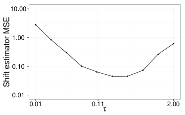
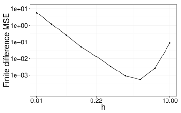
Figure 1: Mean squared error of the Monte Carlo shift estimator (left), as a function of $\tau$, and of the FD estimator (right) as a function of $h$, on the model of Example 2. These have been obtained based on $100$ independent experiments, each using $N=100$, $M=100$, $y=\left(0,0\right)$ and $\theta^{\star}=\left(1,1\right)$, $\Lambda_{x}=\left(1,0.8,0.8,1\right)$ and $\Lambda_{y\mid x}=\left(0.8,0.4,0.4,1\right)$. We see that the bias-variance trade-off leads to an optimal value of $\tau$. On the right, the FD estimator exhibits a similar trade-off, as a function of the perturbation parameter $h$.

3.3 Bias and variance reduction

Lemma 3 shows that the bias of the estimator $S_{N,\tau_{N}}^{(1)}(\theta^{\star})$ is of order $\tau_{N}^{2}$. We show here how a simple modification allows a substantial reduction of the bias, at the cost of a significant variance inflation. The proof is straightforward and thus omitted.

Lemma 5.

Let $\tau_{N}$ be a decreasing sequence going to zero such that $N^{-1/4}=o(\tau_{N})$. Under Assumptions B1-B2, the estimator $2S_{N,\tau_{N}/\sqrt{2}}^{\left(1\right)}(\theta^{\star})-S_{N,\tau_{N}}^{\left(1\right)}(\theta^{\star})$ satisfies

$$\mathbb{E}_{\tau_{N}/\sqrt{2}}\left[2S_{N,\tau_{N}/\sqrt{2}}^{(1)}(\theta^{\star})\right]-\mathbb{E}_{\tau_{N}}\left[S_{N,\tau_{N}}^{(1)}(\theta^{\star})\right]=\nabla\ell\left(\theta^{\star}\right)+o\left(\tau_{N}^{2}\right).$$

When $S_{N,\tau_{N}/\sqrt{2}}^{(1)}(\theta^{\star})$ and $S_{N,\tau_{N}}^{(1)}(\theta^{\star})$ are statistically independent, then the variance of this estimator is

$$\mathbb{V}_{\tau_{N}/\sqrt{2}}\left[2S_{N,\tau_{N}/\sqrt{2}}^{(1)}(\theta^{\star})\right]+\mathbb{V}_{\tau_{N}}\left[S_{N,\tau_{N}}^{(1)}(\theta^{\star})\right]=9\mathbb{V}_{\tau_{N}}\left[S_{N,\tau_{N}}^{(1)}(\theta^{\star})\right]+o\left(\frac{1}{\tau_{N}^{2}N}\right).$$

A similar reasoning can be done to reduce the bias of $S_{N,\tau_{N}}^{(2)}(\theta^{\star})$. We now consider a simple variance reduction technique. We consider the following modification of $S_{N,\tau_{N}}^{(1)}(\theta^{\star})$:

$$\widetilde{S}_{N,\tau_{N}}^{(1)}(\theta^{\star})=\tau_{N}^{-2}\Sigma^{-1}\left(\sum_{i=1}^{N}\hat{W}^{i}\theta^{i}-\frac{1}{N}\sum_{i=1}^{N}\theta^{i}\right),$$

where $\theta^{\star}$ has been replaced by the empirical average $N^{-1}\sum_{i=1}^{N}\theta^{i}$, which acts as a control variate. The bias of $\widetilde{S}_{N,\tau_{N}}^{(1)}(\theta^{\star})$ is the same as the bias of $S_{N,\tau_{N}}^{(1)}(\theta^{\star})$. The following lemma gives the variance of $\widetilde{S}_{N,\tau_{N}}^{(1)}(\theta^{\star})$ when $N\to\infty$.

Lemma 6.

Let $\tau_{N}$ be a decreasing sequence going to zero such that $N^{-1/4}=o(\tau_{N})$. Under Assumptions B1-B2, the variance of $\widetilde{S}_{N,\tau_{N}}^{(1)}(\theta^{\star})$ satisfies

$$\mathbb{V}_{\tau_{N}}\left[\widetilde{S}_{N,\tau_{N}}^{(1)}(\theta^{\star})\right]=\frac{1}{\tau_{N}^{2}N}\Sigma^{-1}\upsilon_{M}\left(\theta^{\star}\right)+o\left(\frac{1}{\tau_{N}^{2}N}\right).$$ (19)

An informal proof is provided in Section B.3. From Eq. (19), we see that when $\upsilon_{M}\left(\theta^{\star}\right)$ is small compared to $1$, the variance of $\widetilde{S}_{N,\tau_{N}}^{(1)}(\theta^{\star})$ can be significantly smaller than the variance of $S_{N,\tau_{N}}^{(1)}(\theta^{\star})$. On the other hand, if $\upsilon_{M}\left(\theta^{\star}\right)$ is large compared to $1$, then both estimators have similar variances. By a similar reasoning, we could consider reducing the variance of $S_{N,\tau_{N}}^{(2)}(\theta^{\star})$, by replacing the prior variance $\tau^{2}\Sigma$ in Eq. (13) by an empirical counterpart computed from the sample $(\theta^{1},\ldots,\theta^{N})$.

Example 3.

In the context of Example 2, we compare $S_{N,\tau}^{(1)}\left(\theta^{\star}\right)$ and $\widetilde{S}_{N,\tau}^{(1)}\left(\theta^{\star}\right)$ for various values of $\tau$ and two values of $M$ on Figure 2. The value of $M$ impacts the relative variance $\upsilon_{M}\left(\theta^{\star}\right)$ of the likelihood estimator $\widehat{\mathcal{L}}(\theta)$, for $\theta$ around $\theta^{\star}$. We see that the control variates within $\widetilde{S}_{N,\tau}^{(1)}\left(\theta^{\star}\right)$ make a significant improvement when the relative variance of $\widehat{\mathcal{L}}(\theta)$ is small ($M=1000$), but that their effect is barely noticeable when the relative variance of $\widehat{\mathcal{L}}(\theta)$ is large ($M=1$).

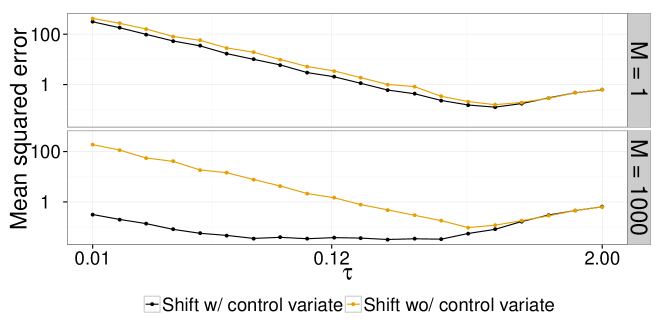
Figure 2: Mean squared error of the Monte Carlo shift estimators $S_{N,\tau}^{(1)}\left(\theta^{\star}\right)$ and $\widetilde{S}_{N,\tau}^{(1)}\left(\theta^{\star}\right)$, respectively without and with control variates, as a function of $\tau$, on the model of Example 2. The top panel compares the estimators when $M=1$, i.e. the relative variance of the likelihood estimator $\upsilon_{M}\left(\theta^{\star}\right)$ is large. The bottom panel compares the estimators when $M=1000$, i.e. the relative variance of the likelihood estimator $\upsilon_{M}\left(\theta^{\star}\right)$ is small. These have been obtained based on $100$ independent experiments, each using $N=100$, $y=\left(0,0\right)$ and $\theta^{\star}=\left(1,1\right)$, $\Lambda_{x}=\left(1,0.8,0.8,1\right)$ and $\Lambda_{y\mid x}=\left(0.8,0.4,0.4,1\right)$. We see that the control variates improve the estimator by an order of magnitude when $\upsilon_{M}\left(\theta^{\star}\right)$ is small, but has no effect when $\upsilon_{M}\left(\theta^{\star}\right)$ is large.

We next implement the bias reduction technique described in Lemma 5, on top of the control variates. We thus compare $\widetilde{S}_{N,\tau}^{(1)}\left(\theta^{\star}\right)$ and $2\widetilde{S}_{N,\tau/\sqrt{2}}^{(1)}\left(\theta^{\star}\right)-\widetilde{S}_{N,\tau}^{(1)}\left(\theta^{\star}\right)$. The results are shown on Figure 3. We see that the bias reduction technique leads to a decrease in the squared bias for large values of $\tau$, where the systematic bias of $S_{\tau}^{(1)}(\theta^{\star})$ dominates the Monte Carlo bias. For smaller values of $\tau$, the bias reduction technique appears detrimental. On the other hand, the variance is always increased by a constant factor.

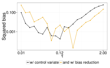
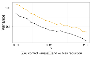
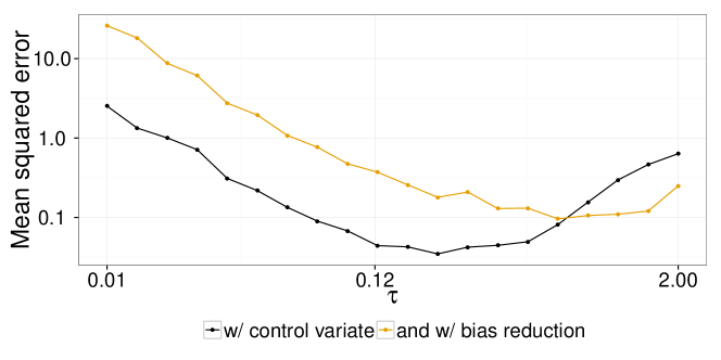
Figure 3: Squared bias (top left) and variance (top right) and mean squared error (bottom) of the Monte Carlo shift estimators, with control variates, with and without bias reduction, as a function of $\tau$, on the model of Example 2. These have been obtained based on $100$ independent experiments, each using $N=100$, $M=100$, $y=\left(0,0\right)$ and $\theta^{\star}=\left(1,1\right)$, $\Lambda_{x}=\left(1,0.8,0.8,1\right)$ and $\Lambda_{y\mid x}=\left(0.8,0.4,0.4,1\right)$. We see that the bias reduction technique allows a decrease of the bias for larger values of $\tau$, where the systematic bias dominates the Monte Carlo bias. On the other hand, it increases the variance by a constant factor. In this example, the minimum mean squared error is achieved without the bias reduction technique.

3.4 Effect of the dimension of the parameter

We now consider a $d$-dimensional parameter space. As described in Section 3.1, we can either estimate the derivatives jointly (using $S_{N,\tau_{N}}^{(1)}(\theta^{\star})$) or component-wise (using $S_{N,\tau_{N}}^{(1)\otimes}(\theta^{\star})$). We wonder whether to use $S_{N,\tau_{N}}^{(1)}\left(\theta^{\star}\right)$ or $S_{N,\tau_{N}}^{(1)\otimes}(\theta^{\star})$. For the latter, Lemma 3 leads to the bias and variance expressions:

$$\mathbb{E}_{\tau_{N},k}\left[\left\{S_{N,\tau_{N}}^{(1)\otimes}(\theta^{\star})\right\}_{k}\right] =\nabla_{k}\ell\left(\theta^{\star}\right)+\tau_{N}^{2}\Sigma_{kk}\left(\frac{1}{2}\nabla_{kkk}^{3}\ell\left(\theta^{\star}\right)+\nabla_{kk}^{2}\ell\left(\theta^{\star}\right)\nabla_{k}\ell\left(\theta^{\star}\right)\right)+o\left(\tau_{N}^{2}\right),$$ (20)

$$\mathbb{V}_{\tau_{N},k}\left[\left\{S_{N,\tau_{N}}^{(1)\otimes}(\theta^{\star})\right\}_{k}\right] =\frac{1}{\tau_{N}^{2}N}\Sigma_{kk}^{-1}\left(1+\upsilon_{M}\left(\theta^{\star}\right)\right)+o\left(\frac{1}{\tau_{N}^{2}N}\right).$$ (21)

For comparison, we thus need a similar result for $S_{N,\tau}^{(1)}\left(\theta^{\star}\right)$. The following result is a generalization of Lemma 3 in the $d$-dimensional setting.

Lemma 7.

Let $\tau_{N}$ be a decreasing sequence going to zero such that $N^{-1/4}=o(\tau_{N})$. Under Assumptions B1-B2, the bias and variance of $S_{N,\tau_{N}}^{(1)}\left(\theta^{\star}\right)$ can be written, for $k\in\left\{1,\ldots,d\right\}$:

$$\mathbb{E}_{\tau_{N}}\left[\left\{S_{N,\tau_{N}}^{(1)}\left(\theta^{\star}\right)\right\}_{k}\right] =\nabla_{k}\ell\left(\theta^{\star}\right)+\tau_{N}^{2}\sum_{i=1}^{d}\sum_{j=1}^{d}\left(\frac{1}{2}\nabla_{ijk}^{3}\ell\left(\theta^{\star}\right)+\nabla_{ik}^{2}\ell\left(\theta^{\star}\right)\nabla_{j}\ell\left(\theta^{\star}\right)\right)\Sigma_{ij}+o\left(\tau_{N}^{2}\right),$$ (22)

$$\mathbb{V}_{\tau_{N}}\left[\left\{S_{N,\tau_{N}}^{(1)}\left(\theta^{\star}\right)\right\}_{k}\right] =\frac{1}{\tau_{N}^{2}N}\Sigma_{kk}^{-1}\left(1+\upsilon_{M}\left(\theta^{\star}\right)\right)+o\left(\frac{1}{\tau_{N}^{2}N}\right).$$ (23)

In the statement of the above lemma, Assumptions B1-B2 need to be interpreted component-wise. The proof is given in Section B.4. Note that the estimator $S_{N,\tau_{N}}^{(1)}\left(\theta^{\star}\right)$ has correlations between its components, whereas the components of $S_{N,\tau_{N}}^{(1)\otimes}(\theta^{\star})$ are independent. The correlations between components of $S_{N,\tau_{N}}^{(1)}\left(\theta^{\star}\right)$ are omitted from the above lemma for sake of brevity. Some guidelines to evaluate these correlations are given in Section B.4.

From Eq. (20) and Eq. (22), we see that the bias has fewer terms when the estimation is performed element-wise rather than jointly. In particular, for general covariance matrices $\Sigma$, the leading term in the bias expressed in Eq. (22) is quadratic in $d$. If one uses a diagonal matrix for $\Sigma$, then the bias is only linear in $d$. It could happen that these $d$ terms compensate each other, but in general, these equations indicate that it is better to estimate the score element-wise in terms of bias. Indeed, for the optimal choice $\tau_{N}=N^{-1/6}$, the bias is in $N^{-1/3}$, and thus dividing the bias of $S_{N,\tau_{N}}^{(1)}\left(\theta^{\star}\right)$ by $d$ would cost more than a $d$-fold increase in computational cost, that corresponds to the cost of $S_{N,\tau_{N}}^{(1)\otimes}(\theta^{\star})$ for the same values of $N$ and $M$. Note that we expect the use of the bias reduction technique described in Lemma 5 to be more significant for $S_{N,\tau_{N}}^{(1)}\left(\theta^{\star}\right)$ than for $S_{N,\tau_{N}}^{(1)\otimes}(\theta^{\star})$.

From Eq. (21) and Eq. (23), we see that the leading term in the variance is the same whether the estimation is performed element-wise or jointly. Given that performing the estimation jointly is $d$ times faster for fixed values of $N$ and $M$, it is therefore advantageous to perform the estimation jointly, in terms of variance. The term $\upsilon_{M}\left(\theta^{\star}\right)$ itself is typically increasing with $d$, or conversely, $M$ has to be increased with $d$ in order for $\upsilon_{M}\left(\theta^{\star}\right)$ to be stable. If we consider the simple case of a likelihood function that factorizes into $d$ independent terms:

$$\mathcal{L}\left(\theta\right)=\prod_{k=1}^{d}\mathcal{L}_{k}(\theta_{k}),$$

then, for a given $\theta$, estimating each term $\mathcal{L}_{k}(\theta_{k})$ independently with $\widehat{\mathcal{L}}_{k}(\theta_{k})$ leads to the variance

$$\mathbb{V}\left[\frac{\widehat{\mathcal{L}}(\theta)}{\mathcal{L}(\theta)}\right] =\mathbb{E}\left[\left(\frac{\widehat{\mathcal{L}}(\theta)}{\mathcal{L}(\theta)}\right)^{2}\right]-1=\prod_{i=1}^{d}\left(1+\mathbb{V}\left[\frac{\widehat{\mathcal{L}}_{k}(\theta_{k})}{\mathcal{L}_{k}(\theta_{k})}\right]\right)-1$$

$$=\prod_{i=1}^{d}\left(1+\frac{\upsilon}{M}\right)-1\leq\exp\upsilon-1$$

assuming that $\upsilon/M$ is the relative variance of each estimator $\widehat{\mathcal{L}}_{k}(\theta_{k})$, that $M=d$, and noting that $\left(1+\upsilon/d\right)^{d}\leq\exp\upsilon$ for all $d$. Thus the relative variance of $\widehat{\mathcal{L}}(\theta)$ is upper bounded by a constant when $M$ is chosen to increase linearly in $d$. A similar behavior has been demonstrated for likelihood estimators obtained by particle methods for specific models [4, 6]. In general, the relative variance of the likelihood estimator is expected to increase at least linearly with $d$.

3.5 Robustness to high variance in the likelihood estimator

We now consider the behavior of the shift estimators when the relative variance $\upsilon_{M}\left(\theta^{\star}\right)$ of the likelihood estimator $\widehat{\mathcal{L}}(\theta)$ is large. Note that the randomness of Monte Carlo shift estimators occurs in the form of weighted averages of draws from $\mathcal{N}(\theta^{\star},\tau^{2}\Sigma)$, with the likelihood estimator appearing only in the weights. When the relative variance increases, the normalized weights $(\hat{W}^{1},\ldots\hat{W}^{N})$ used in the Monte Carlo shift estimators of Eq. (12) and Eq. (13) become more and more unbalanced, one of the normalized weights typically getting close to one while all the others are nearing zero. As a result, the weighted average $\sum_{i=1}^{N}\hat{W}^{i}\theta^{i}$ reduces to one draw $\theta^{i}$ that corresponds to the only significant normalized weight. Then the difference between $\sum_{i=1}^{N}\hat{W}^{i}\theta^{i}$ and $\theta^{\star}$ is of order $\tau$ and the bias of the estimator $S_{N,\tau}^{(1)}(\theta^{\star})$ can then be bounded by a term of order $\tau^{-1}$, independently of $\upsilon_{M}\left(\theta^{\star}\right)$. Similarly, the following lemma gives an upper bound on the variance of $S_{N,\tau}^{(1)}(\theta^{\star})$.

Lemma 8.

Assume that the likelihood estimator $\widehat{\mathcal{L}}(\theta)$ is unbiased and has a relative variance equal to $\upsilon_{M}\left(\theta^{\star}\right)$. Let $\tau$, $N$ and $M$ be fixed. There exists a constant $C$ independent of $\upsilon_{M}\left(\theta^{\star}\right)$ and $\tau$ such that

$$\mathbb{V}_{\tau}\left[S_{N,\tau}^{(1)}(\theta^{\star})\right]\leq C\tau^{-4}.$$

A proof is provided in Section B.5. The constant $C$ depends implicitly on $N$, although we conjecture that a more sophisticated proof might be able to remove this dependency. For the second order derivative, the estimator $S_{N,\tau}^{(2)}(\theta^{\star})$ of Eq. (13) is very close to $0$ when only one of the normalized weights is significant, and thus the variance of $S_{N,\tau}^{(2)}(\theta^{\star})$ is very small. Since the real posterior variance is of order $\tau^{2}$, the bias of $S_{N,\tau}^{(2)}(\theta^{\star})$ would then be of order $\tau^{-2}$, and thus $S_{N,\tau}^{(2)}(\theta^{\star})$ would have a mean squared error bounded by a term in $C\tau^{-4}$, for another constant $C$ that does not depend on $\upsilon_{M}\left(\theta^{\star}\right)$.

Thus the Monte Carlo shift estimators benefit from some robustness to the relative variance $\upsilon_{M}\left(\theta^{\star}\right)$ of the likelihood estimator. This will prove a significant advantage over FD estimators, as illustrated in the following example.

Example 4.

To simulate a setting where the relative variance increases to infinity in the context of Example 2, we consider the case where the variance of the observation distribution $Y\mid X=x$, becomes smaller and smaller. We thus introduce a scaling factor $\lambda\in\left(0,1\right)$ and $V_{y\mid x}=\lambda\Lambda_{y\mid x}^{-1},$ and we set $V_{x}=\Lambda_{y}^{-1}-V_{y\mid x}$. Hence the matrix $\Lambda_{y}=(V_{x}+V_{y\mid x})^{-1}$ is the same for all $\lambda$, and thus the score is unchanged, but the Monte Carlo procedure struggles more and more as $\lambda$ approaches zero. Figure 4 represents the behavior of the shift estimator $S_{N,\tau}^{(1)}\left(\theta^{\star}\right)$, the version with control variates $\widetilde{S}_{N,\tau}^{(1)}\left(\theta^{\star}\right)$, and the FD estimator $D_{h}^{(1)}\left(\theta^{\star}\right)$, where the computational effort has been matched, thus $D_{h}^{(1)}\left(\theta^{\star}\right)$ uses $N\times M/4$ samples for each log-likelihood estimate. We see that the shift estimators get worse when $\lambda$ goes to very small values, but that the errors are eventually bounded, whereas the mean squared error of the FD estimator going to infinity.

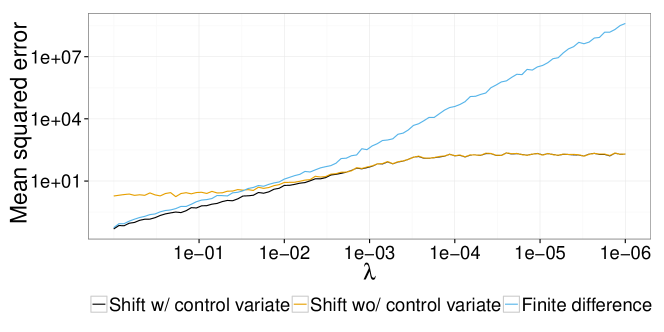
Figure 4: Mean squared error of the Monte Carlo shift estimators with and without covariates, and the FD estimator as a function of $\lambda$, which parametrizes the signal to noise ratio in Example 2. The smaller the $\lambda$, the worse the estimation of the likelihood estimator. We see that the shift estimators only degrade up to a certain point when $\lambda$ decreases. On the other hand, the variance of the FD estimator goes to infinity when $\lambda$ decreases. These have been obtained based on $100$ independent experiments, each using $N=100$, $M=100$, $y=\left(0,0\right)$ and $\theta^{\star}=\left(1,1\right)$, $\Lambda_{x}=\left(1,0.8,0.8,1\right)$ and $\Lambda_{y\mid x}=\left(0.8,0.4,0.4,1\right)$. The FD estimator uses $N\times M/4$ samples for each log-likelihood estimate, so that the computational comparison is fair. The perturbation parameters have been set to $\tau=0.1$ and $h=0.1$, arbitrarily.

3.6 Comparison with finite difference type estimators

In order to compare Monte Carlo shift estimators with FD type estimators, we first recall some of their standard properties. We will assume the following properties of the log-likelihood estimator $\log\widehat{\mathcal{L}}(\theta)$, for any $\theta$:

$$\mathbb{E}\left[\log\widehat{\mathcal{L}}(\theta)\right] =\ell(\theta),$$

$$\mathbb{V}\left[\log\widehat{\mathcal{L}}(\theta)\right] =\ell(\theta)^{2}U_{M}\left(\theta\right),$$

where $U_{M}\left(\theta\right)$ thus quantifies the relative variance of $\log\widehat{\mathcal{L}}(\theta)$ for all $\theta$, and $M$ is a tuning parameter. We further assume that $U_{M}\left(\theta\right)$ is equal to $U_{M}\left(\theta^{\star}\right)$ for all $\theta$ in a neighborhood of $\theta^{\star}$; see [2] for similar assumptions and results. We make the following assumption on the log-likelihood.

• C1. The log-likelihood $\ell$ is four times continuously differentiable, and there exists $K<\infty$ and $\delta>0$ such that $\left|\nabla_{ijkl}^{4}\ell(\theta)\right|\leq K$ for all $\theta$ such that $||\theta-\theta^{\star}||\leq\delta$, for all $i,j,k,l\in\left\{1,\ldots,d\right\}$.

The following results hold for the component-wise FD estimator $D_{h}^{(1)\otimes}(\theta^{\star})$.

Lemma 9.

Let $h_{M}$ be a decreasing sequence going to zero. Under condition C1, for each $k\in\left\{1,\ldots,d\right\}$, the $k$-th component of $D_{h}^{(1)\otimes}(\theta^{\star})$ satisfies

$$\mathbb{E}\left[\left\{D_{h_{M}}^{(1)\otimes}(\theta^{\star})\right\}_{k}\right] =\nabla_{k}\ell\left(\theta^{\star}\right)+\frac{h_{M}^{2}}{6}\nabla_{kkk}^{3}\ell(\theta^{\star})+o(h_{M}^{2}),$$ (24)

$$\mathbb{V}\left[\left\{D_{h_{M}}^{(1)\otimes}(\theta^{\star})\right\}_{k}\right] =\frac{1}{4h_{M}^{2}}U_{M}\left(\theta^{\star}\right)\left(\ell(\theta^{\star}+h_{M})^{2}+\ell(\theta^{\star}-h_{M})^{2}\right).$$ (25)

If we further assume that $U_{M}\left(\theta^{\star}\right)=U\left(\theta^{\star}\right)/M$ for some $U\left(\theta^{\star}\right)>0$, the mean squared error can be optimized by choosing $h_{M}=M^{-1/6}$, and is then of order $M^{-2/3}$.

A proof is provided in Section B.6. We thus obtain the same rate of convergence for the FD estimator when $M\to\infty$ than for the shift estimator when $N\to\infty$ as in Lemma 3.

We now recall the impact of the dimension on FD estimators. For the component-wise FD estimator $D_{h_{M}}^{(1)\otimes}(\theta^{\star})$, we obtain the same behavior as the component-wise Monte Carlo shift estimator $S_{N,\tau_{N}}^{(1)\otimes}(\theta^{\star})$. For the SP estimator $D_{N,h_{N}}^{(1)}(\theta^{\star})$ of Eq. (16), we make the following assumption.

• C2. The perturbation $\varepsilon^{i}=(\varepsilon_{1}^{i},\ldots,\varepsilon_{d}^{i})$, for $i\in\left\{1,\ldots,N\right\}$, is such that the components $\varepsilon_{k}^{i}$, for $k\in\left\{1,\ldots,d\right\}$, are drawn independently from the uniform distribution on $\left\{-1,1\right\}$.

Lemma 10.

Let $h_{N}$ be a decreasing sequence going to zero. Under Assumptions C1-C2, the SP estimator $D_{N,h_{N}}^{(1)}(\theta^{\star})$ satisfies the following properties,

$$\mathbb{E}\left[\left\{D_{N,h_{N}}^{(1)}(\theta^{\star})\right\}_{k}\right] =\nabla_{k}\ell\left(\theta^{\star}\right)+\frac{h_{N}^{2}}{6}\sum_{1\leq i_{1},i_{2},i_{3}\leq d}\nabla_{i_{1}i_{2}i_{3}}^{3}\ell(\theta^{\star})\mathbb{E}\left[\frac{\varepsilon_{i_{1}}\varepsilon_{i_{2}}\varepsilon_{i_{3}}}{\varepsilon_{k}}\right]+o(h_{N}^{2}),$$ (26)

$$\mathbb{V}\left[\left\{D_{N,h_{N}}^{(1)}(\theta^{\star})\right\}_{k}\right] =\frac{U_{M}\left(\theta^{\star}\right)}{2Nh_{N}^{2}}\ell(\theta^{\star})^{2}+o\left(\frac{1}{Nh_{N}^{2}}\right),$$ (27)

and there is a constant $C(\theta^{\star})$ such that

$$\left|\sum_{1\leq i_{1},i_{2},i_{3}\leq d}\nabla_{i_{1}i_{2}i_{3}}^{3}\ell(\theta^{\star})\mathbb{E}\left[\frac{\varepsilon_{i_{1}}\varepsilon_{i_{2}}\varepsilon_{i_{3}}}{\varepsilon_{k}}\right]\right|\leq C(\theta^{\star})\times d.$$

A short proof is given in Section B.6. Similar results could be obtained for other distributions of the perturbation variable $\varepsilon$, as long as the distribution is symmetric, with finite moments and finite inverse moments, which precludes the normal distribution. From Lemma 10, we see that the bias term is linear in $d$. On the other hand, the variance term depends on $d$ only through the relative variance $U_{M}$ of the log-likelihood estimator. We thus conclude that the bias and variance of $D_{N,h_{N}}^{(1)}(\theta^{\star})$ behave similarly as those of the Monte Carlo shift estimator $S_{N,\tau_{N}}^{(1)}(\theta^{\star})$, with respect to the dimension $d$ (compare Lemma 10 and Lemma 7 with $\Sigma$ diagonal). Although omitted here, the estimators of the second derivatives, $D_{N,h_{N}}^{(2)}(\theta^{\star})$ and $D_{N,h_{N}}^{(2)\otimes}(\theta^{\star})$, could be studied similarly, and we would also find the same convergence rates as for $S_{N,h_{N}}^{(2)}(\theta^{\star})$ and $S_{N,h_{N}}^{(2)\otimes}(\theta^{\star})$. The Monte Carlo shift estimators thus exhibit the same convergence rates in general as FD type estimators including simultaneous perturbations.

The non-asymptotic regime of both classes of estimators is different. We have seen in Section 3.5 that the Monte Carlo shift estimators always have a bounded variance, irrespective of the relative variance $\upsilon_{M}\left(\theta^{\star}\right)$ of the likelihood estimator. On the other hand, the variance of FD type estimators increases linearly with the relative variance $U_{M}$ of the log-likelihood estimator, possibly to infinity, as was illustrated in Example 4.

Remark 3.

In practice we typically either have access to an unbiased estimator of the likelihood, or to an unbiased estimator of the log-likelihood. Suppose that we have access to an unbiased estimator of the likelihood, such as the one obtained by particle filters in the context of state-space models. Taking the logarithm of the estimator yields a log-likelihood estimator with a bias of order $M^{-1}$, where $M$ is, say, the number of particles. We can see from the proof of Lemma 9 that it does not change the overall convergence rate of the component-wise FD estimator $D_{h_{M}}^{(1)\otimes}(\theta^{\star})$, as long as $M^{-1}=o(h_{M}^{2})$, which ensures that the Monte Carlo bias vanishes faster than the systematic bias coming from the Taylor expansion. On the other hand, averaging over $N$ draws as in the SP estimator $D_{N,h_{N}}^{(1)}(\theta^{\star})$ does not reduce the bias, which would be of constant order $M^{-1}$ when $N\to\infty$. Thus, one might want to decide which score estimator to use according to which quantity can be unbiasedly estimated.

4 Monte Carlo shift estimators for latent variable models

4.1 Extended likelihood function and shift estimators

We discuss here an alternative to the shift estimators introduced in Section 2 which is applicable whenever the log-likelihood function $\ell\left(\theta\right)$ arises from multiple and/or multivariate observations. Given observations $y_{1:T}=\left(y_{1},\ldots y_{T}\right)$, we can indeed always decompose the log-likelihood as a sum of terms:

$$\ell(\theta)=\log\thinspace p(y_{1:T}\mid\theta)=p(y_{1}\mid\theta)+\sum_{t=2}^{T}\log\thinspace p(y_{t}\mid y_{1:t-1},\theta).$$ (28)

Directly applying the shift estimator yields the estimators $S_{\tau}^{(1)}\left(\theta^{\star}\right)$ and $S_{\tau}^{(2)}\left(\theta^{\star}\right)$ of Theorem 1. An alternative exploiting the predictive decomposition of Eq. (28) is possible, as advocated in [13, 14] for the score vector. It proceeds as follows. We introduce a $T\times d$ dimensional parameter $\theta_{1:T}=\left(\theta_{1},\ldots\theta_{T}\right)$, where $\theta_{t}\in\mathbb{R}^{d}$, and denote by $\theta^{[T]}=(\theta,\ldots,\theta)$ the vector made of $T$ copies of $\theta$. We then define the following artificial log-likelihood function $\bar{\ell:}\,\mathbb{R}^{d\times T}\rightarrow\mathbb{R}$,

$$\bar{\ell}\left(\theta_{1:T}\right)=p(y_{1}\mid\theta_{1})+\sum_{t=2}^{T}\log p(y_{t}\mid y_{1:t-1},\theta_{t}).$$ (29)

which satisfies $\bar{\ell}\left(\theta^{[T]}\right)=\ell\left(\theta\right)$ for all $\theta$. Then the chain rule, applied to $\ell=\bar{\ell}\circ m_{T}$ where $m_{T}:\theta\mapsto\theta^{[T]}$, yields

$$\nabla\ell\left(\theta\right) =\sum_{t=1}^{T}\nabla_{t}\bar{\ell}\left(\theta^{[T]}\right),$$

$$\nabla^{2}\ell\left(\theta\right) =\sum_{s=1}^{T}\sum_{t=1}^{T}\nabla_{st}^{2}\bar{\ell}\left(\theta^{[T]}\right).$$

Therefore, an estimator of $\nabla\ell\left(\theta^{\star}\right)$, respectively $\nabla^{2}\ell\left(\theta^{\star}\right)$, can be obtained by summing the components of an estimator of the extended gradient vector $\nabla\bar{\ell}(\theta^{\star[T]})$, respectively of an estimator of the extended Hessian matrix $\nabla^{2}\bar{\ell}(\theta^{\star[T]})$. Now, we can obtain such estimators by introducing a prior distribution $\mathcal{N}\left(\theta^{\star[T]},\tau^{2}\bar{\Sigma}\right)$, where $\bar{\Sigma}$ is a $dT\times dT$ covariance matrix, and using Theorem 1,

$$\tau^{-2}\bar{\Sigma}^{-1}\left(\check{\mathbb{E}}_{\tau}^{[T]}\left[\bar{\Theta}\right]-\theta^{\star[T]}\right) = \nabla\bar{\ell}\left(\theta^{\star[T]}\right)+\mathcal{O}\left(\tau^{2}\right),$$ (30)

$$\tau^{-4}\bar{\Sigma}^{-1}\left(\check{\mathbb{V}}_{\tau}^{[T]}\left[\bar{\Theta}\right]-\tau^{2}\bar{\Sigma}\right)\bar{\Sigma}^{-1} = \nabla^{2}\bar{\ell}\left(\theta^{\star[T]}\right)+\mathcal{O}\left(\tau^{2}\right).$$ (31)

where $\check{\mathbb{E}}_{\tau}^{[T]}\left[\bar{\Theta}\right]$ and $\check{\mathbb{V}}_{\tau}^{[T]}\left[\bar{\Theta}\right]$ refers to the posterior mean and variance in the extended model. Summing the $T$ $d$-dimensional blocks of the estimator of $\nabla\bar{\ell}\left(\theta^{\star[T]}\right)$, respectively the $T^{2}$ $d\times d$-dimensional blocks of the estimator of $\nabla^{2}\bar{\ell}(\theta^{\star[T]})$, we obtain

$$\bar{S}_{\tau}^{(1)}\left(\theta^{\star}\right) = \tau^{-2}\sum_{t=1}^{T}\left\{\bar{\Sigma}^{-1}\left(\check{\mathbb{E}}_{\tau}^{[T]}\left[\bar{\Theta}\right]-\theta^{\star[T]}\right)\right\}_{t}=\nabla\ell\left(\theta^{\star}\right)+\mathcal{O}\left(\tau^{2}\right),$$ (32)

$$\bar{S}_{\tau}^{(2)}\left(\theta^{\star}\right) = \tau^{-4}\sum_{s=1}^{T}\sum_{t=1}^{T}\left\{\bar{\Sigma}^{-1}\left(\check{\mathbb{V}}_{\tau}^{[T]}\left[\bar{\Theta}\right]-\tau^{2}\bar{\Sigma}\right)\bar{\Sigma}^{-1}\right\}_{st}=\nabla^{2}\ell(\theta^{\star})+\mathcal{O}\left(\tau^{2}\right),$$ (33)

where here $\left\{v\right\}_{t}$ denotes the $t$-th $d$-dimensional block of a $dT$-dimensional vector and $\left\{v\right\}_{st}$ denotes the $(s,t)$-th $d\times d$-dimensional block of a $dT\times dT$-dimensional matrix.

4.2 Independent latent variable models

To motivate the introduction of the alternative shift estimators of Eq. (32) and Eq. (33), consider the case where the log-likelihood satisfies

$$\ell(\theta)=\sum_{t=1}^{T}\ell_{t}(\theta),$$ (34)

where $\ell_{t}(\theta)=\log\thinspace p(y_{t}\mid\theta)=\log\thinspace\mathcal{L}{}_{t}(\theta)$. Assume that the covariance matrix $\bar{\Sigma}$, a $dT\times dT$ matrix, is chosen to be block diagonal, where each diagonal block is equal to $\Sigma$, a $d\times d$ covariance matrix. That is, the artificial prior assigned to $\Theta_{1:T}$ assumes that its components $\Theta_{t}$ are independent and identically distributed as $\mathcal{N}\left(\theta^{\star},\tau^{2}\Sigma\right)$. Then the shift estimators of Eq. (32) and Eq. (33) are equal to

$$\bar{S}_{\tau}^{(1)}\left(\theta^{\star}\right) = \tau^{-2}\Sigma^{-1}\sum_{t=1}^{T}\left(\check{\mathbb{E}}_{\tau,t}\left[\Theta\right]-\theta^{\star}\right),$$ (35)

$$\bar{S}_{\tau}^{(2)}\left(\theta^{\star}\right) = \tau^{-4}\Sigma^{-1}\left(\sum_{t=1}^{T}\left(\check{\mathbb{V}}_{\tau,t}\left[\Theta\right]-\tau^{2}\Sigma\right)\right)\Sigma^{-1},$$ (36)

where $\check{\mathbb{E}}_{\tau,t}$ and $\check{\mathbb{V}}_{\tau,t}$ denote the expectation and variance under the artificial posterior associated to the prior $\mathcal{N}\left(\theta^{\star},\tau^{2}\Sigma\right)$ and the likelihood $\mathcal{L}_{t}(\theta)$.

We compare here the original shift estimator $S_{\tau}^{(1)}\left(\theta^{\star}\right)$ and its approximation $S_{N,\tau}^{(1)}\left(\theta^{\star}\right)$ to $\bar{S}_{\tau}^{(1)}\left(\theta^{\star}\right)$ and its approximation $\bar{S}_{N,\tau}^{(1)}\left(\theta^{\star}\right)$. The bias of $S_{\tau}^{(1)}\left(\theta^{\star}\right)$ obtained in Theorem 1, which is also the leading term in the bias of $S_{N,\tau}^{(1)}\left(\theta^{\star}\right)$ obtained in Lemma 7, can be written, for the $k$-th component of the gradient.

$$\tau^{2}\sum_{i=1}^{d}\sum_{j=1}^{d}\left(\frac{1}{2}\nabla_{ijk}^{3}\ell\left(\theta^{\star}\right)+\nabla_{ik}^{2}\ell\left(\theta^{\star}\right)\nabla_{j}\ell\left(\theta^{\star}\right)\right)\Sigma_{ij}$$

$$= \tau^{2}\sum_{i=1}^{d}\sum_{j=1}^{d}\left(\frac{1}{2}\sum_{t=1}^{T}\nabla_{ijk}^{3}\ell_{t}\left(\theta^{\star}\right)+\left(\sum_{t=1}^{T}\nabla_{ik}^{2}\ell_{t}\left(\theta^{\star}\right)\right)\left(\sum_{t=1}^{T}\nabla_{j}\ell_{t}\left(\theta^{\star}\right)\right)\right)\Sigma_{ij}$$

where we have used the specific form of the log-likelihood of Eq. (34). It thus increases quadratically with $T$. The variance of $S_{N,\tau}^{(1)}\left(\theta^{\star}\right)$, according to Lemma 7, is led by $\tau^{-2}N^{-1}\Sigma_{kk}^{-1}(1+\upsilon_{M}\left(\theta^{\star}\right))$ for the $k$-th component, and thus increases with $T$ insofar as $\upsilon_{M}\left(\theta^{\star}\right)$ does; typically $\upsilon_{M}\left(\theta^{\star}\right)$ would increase at least linearly with $T$. Thus, the mean squared error would be dominated by the squared bias term in $T^{4}$ when $T$ increases.

On the other hand, the bias of $\bar{S}_{\tau}^{(1)}\left(\theta^{\star}\right)$ can be written

$$\tau^{2}\sum_{t=1}^{T}\sum_{i=1}^{d}\sum_{j=1}^{d}\left(\frac{1}{2}\nabla_{ijk}^{3}\ell_{t}\left(\theta^{\star}\right)+\nabla_{ik}^{2}\ell_{t}\left(\theta^{\star}\right)\nabla_{j}\ell_{t}\left(\theta^{\star}\right)\right)\Sigma_{ij}$$

which only increases linearly with $T$. The variance of $\bar{S}_{N,\tau}^{(1)}\left(\theta^{\star}\right)$ is led by the term $\tau^{-2}N^{-1}\Sigma_{kk}^{-1}\sum_{t=1}^{T}(1+\upsilon_{M,t})$, where $\upsilon_{M,t}$ is the relative variance of the partial likelihood estimator $\widehat{\mathcal{L}}_{t}(\theta)$, which can be assumed to be constant. Thus the variance increases linearly with $T$, similarly to the variance of $S_{N,\tau}^{(1)}\left(\theta^{\star}\right)$. Overall the mean squared error of $\bar{S}_{N,\tau}^{(1)}\left(\theta^{\star}\right)$ is thus expected to become lower than that of $S_{N,\tau}^{(1)}\left(\theta^{\star}\right)$ when $T$ increases.

Furthermore, consider the case where one of the $\ell_{t}$ is particularly hard to estimate, for instance because $y_{t}$ is an outlier. Denote its index by $t$ and imagine the extreme scenario where the relative variance of $\mathcal{\widehat{L}}_{t}(\theta^{\star})$ is infinite. Then the relative variance of the full likelihood estimator $\widehat{\mathcal{L}}(\theta^{\star})$ would also be infinite. Using $S_{N,\tau}^{(1)}\left(\theta^{\star}\right)$ would certainly result in poor performances, although the reasoning of Lemma 8 guarantees a finite variance. Finite difference type estimators would have an infinite variance in this setting. On the other hand, if we use $\bar{S}_{N,\tau}^{(1)}\left(\theta^{\star}\right)$, the term corresponding to $\ell_{t}$ would be poorly estimated, but with a finite variance. If all the other terms are correctly estimated, and if their norms are large enough to dominate the poorly estimated term, then it is possible that $\bar{S}_{N,\tau}^{(1)}\left(\theta^{\star}\right)$ would still be satisfactory. This motivates the development of Monte Carlo approximations of $\bar{S}_{\tau}^{(1)}\left(\theta^{\star}\right)$ in the next section, following [13, 14], instead of trying to approximate $S_{\tau}^{(1)}(\theta^{\star})$ directly for state-space models, using particle Markov chain Monte Carlo [1] or SMC² [5].

Example 5.

We augment Example 2 with $T$ observations $Y_{1},\ldots,Y_{T}$, and $T$ latent variables $X_{1},\ldots,X_{T}$, independent and identically distributed. The derivatives of the log-likelihood at $\theta^{\star}$ are then

$$\nabla\ell(\theta^{\star})=-\Lambda_{y}\sum_{t=1}^{T}(\theta^{\star}-y_{t})\quad\text{and}\quad\nabla^{2}\ell(\theta^{\star})=-T\Lambda_{y}.$$

The original shift estimators are given by

$$S_{\tau}^{(1)}\left(\theta^{\star}\right) =\tau^{-2}\Sigma^{-1}(\tau^{-2}\Sigma^{-1}+T\Lambda_{y})^{-1}\left(-\Lambda_{y}\sum_{t=1}^{T}(\theta^{\star}-y_{t})\right),$$

$$S_{\tau}^{(2)}\left(\theta^{\star}\right) =\tau^{-2}\Sigma^{-1}(\tau^{-2}\Sigma^{-1}+T\Lambda_{y})^{-1}\left(-T\Lambda_{y}\right).$$

In one dimension, we can check that the bias of $S_{\tau}^{(1)}\left(\theta^{\star}\right)$ would be equal to $\tau^{2}\Sigma T\Lambda_{y}\nabla\ell(\theta^{\star}),$ which is quadratic in $T$ because $\nabla\ell(\theta^{\star})$ is equal to $-\Lambda_{y}\sum_{t=1}^{T}(\theta^{\star}-y_{t})$. On the other hand, using the extended model, we obtain

$$\bar{S}_{\tau}^{(1)}\left(\theta^{\star}\right) =\sum_{t=1}^{T}\tau^{-2}\Sigma^{-1}(\tau^{-2}\Sigma^{-1}+\Lambda_{y})^{-1}\left(-\Lambda_{y}(\theta^{\star}-y_{t})\right),$$

$$\bar{S}_{\tau}^{(2)}\left(\theta^{\star}\right) =\sum_{t=1}^{T}\tau^{-2}\Sigma^{-1}(\tau^{-2}\Sigma^{-1}+\Lambda_{y})^{-1}\left(-\Lambda_{y}\right).$$

The bias of $\bar{S}_{\tau}^{(1)}\left(\theta^{\star}\right)$ only increases linearly with $T$. A similar bias comparison can be done for the second order derivative.

4.3 State-space models

We now focus on the class of state-space models, which generalizes the model of the previous section. We propose alternative shift estimators in this context and discuss their link to the score estimator proposed in [14]. Let $\left(X_{t},Y_{t}\right)_{t\in\mathbb{N}}$ be a stochastic process such that $\left(X_{t},Y_{t}\right)$ takes values in a measurable space $\mathcal{X\times Y}$. The model is specified as follows: $\left(X_{t}\right)_{t\in\mathbb{N}}$ is a latent Markov process of initial density $\nu\left(x;\theta\right)$ and homogeneous Markov transition density $f\left(\left.x\right|x^{\prime};\theta\right)$ whereas the observations $\left(Y_{t}\right)_{t\in\mathbb{N}}$ are assumed to be conditionally independent given $\left(X_{t}\right)_{t\in\mathbb{N}}$ of conditional density $g\left(\left.y_{t}\right|x_{t};\theta\right)$ (with respect to suitable dominating measures) where $\theta\in\mathbb{R}^{d}$ ; that is $X_{1}\sim\mu\left(\cdot;\theta\right)$ and for $t\geq 1$,

$$\left.X_{t+1}\right|\left(X_{t}=x\right)\sim f\left(\left.\cdot\right|x_{t-1};\theta\right),\quad\left.Y_{t}\right|\left(X_{t}=x_{t}\right)\sim g\left(\left.\cdot\right|x_{t};\theta\right).$$ (37)

It follows that the joint density of $\left(X_{1:T},Y_{1:T}\right)$ is given by

$$p\left(x_{1:T},y_{1:T};\theta\right)=\nu\left(x_{1};\theta\right)\prod\limits_{t=2}^{T}f\left(\left.x_{t}\right|x_{t-1};\theta\right)\prod\limits_{t=1}^{T}g\left(\left.y_{t}\right|x_{t};\theta\right).$$ (38)

For a realization $Y_{1:T}=y_{1:T}$ of the observations, the log-likelihood of function satisfies the decomposition of Eq. (28) where

$$p(y_{t}\mid y_{1:t-1},\theta)=\int g\left(\left.y_{t}\right|x_{t};\theta\right)p\left(\left.x_{t}\right|y_{1:t-1};\theta\right)dx_{t},$$

where $p\left(\left.x_{t}\right|y_{1:t-1};\theta\right)$ denotes the posterior distribution of $X_{t}$ given observations $y_{1:t-1}$. Consider a prior where the components $\Theta_{t}$ of $\Theta_{1:T}$ are assumed independent and identically distributed according to $\mathcal{N}\left(\theta^{\star},\tau^{2}\Sigma\right)$. The shift estimators of Eq. (32) and Eq. (33) can be rewritten after simple manipulations as

$$\bar{S}_{\tau}^{(1)}\left(\theta^{\star}\right) = \tau^{-2}\Sigma^{-1}\sum_{t=1}^{T}\left(\mathbb{E_{\tau}}\left[\Theta_{t}\mid y_{1:T}\right]-\theta^{\star}\right),$$ (39)

$$\bar{S}_{\tau}^{(2)}\left(\theta^{\star}\right) = \tau^{-4}\Sigma^{-1}\left(\sum_{s=1}^{T}\sum_{t=1}^{T}\mathbb{C_{\tau}}\left[\Theta_{s},\Theta_{t}\mid y_{1:T}\right]-\tau^{2}\Sigma T\right)\Sigma^{-1},$$ (40)

where $\mathbb{E_{\tau}}\left[\Theta_{t}\mid y_{1:T}\right]$ and $\mathbb{C_{\tau}}\left[\Theta_{s},\Theta_{t}\mid y_{1:T}\right]$ are the expectation of $\Theta_{t}$, respectively covariance of $\left(\Theta_{s},\Theta_{t}\right)$, under the joint posterior smoothing distribution $p_{\tau}\left(\theta_{1:T},x_{1:T}\mid y_{1:T}\right)$ induced by the artificial state space model with initial distribution $\Theta_{1}\sim\mathcal{N}\left(\theta^{\star},\tau^{2}\Sigma\right),\leavevmode\nobreak\ \left.X_{1}\right|\left(\Theta_{1}=\theta\right)\sim\mu\left(\cdot;\theta\right)$ and satisfying for $t\geq 1$,

$$\Theta_{t+1}\sim\mathcal{N}\left(\theta^{\star},\tau^{2}\Sigma\right),\quad\left.X_{t+1}\right|\left(X_{t}=x_{t},\Theta_{t+1}=\theta_{t+1}\right)\sim f\left(\left.\cdot\right|x_{t};\theta_{t+1}\right),\quad\left.Y_{t}\right|\left(X_{t}=x_{t},\Theta_{t}=\theta_{t}\right)\sim g\left(\left.\cdot\right|x_{t};\theta_{t}\right).$$ (41)

Remark 4.

One could introduce other prior distributions on $\Theta_{1:T}$. For example, one could select $\Theta_{1}\sim\mathcal{N}\left(\theta^{\star},\tau^{2}\Sigma\right)$ and for $t\geq 1$

$$\Theta{}_{t+1}-\theta^{\star}=\rho\left(\Theta{}_{t}-\theta^{\star}\right)+V_{t+1},\quad V_{t+1}\sim\mathcal{N}\left(0,\upsilon^{2}\Sigma\right),$$ (42)

where $\rho$ is a scalar, $\left|\rho\right|<1$ and $\tau^{2}=\upsilon^{2}/\left(1-\rho^{2}\right)$. In Appendix C, we provide for this prior distribution the expressions of the shift estimators of Eq. (32) and Eq. (33). When $\rho\rightarrow 1^{-}$, we retrieve informally the score estimator proposed in [14] as

$$\underset{\rho\rightarrow 1^{-}}{\lim}\bar{S}_{\tau}^{(1)}\left(\theta^{\star}\right) \thickapprox \tau^{-2}\Sigma^{-1}\mathbb{E_{\tau}}\left[\Theta_{T}\mid y_{1:T}\right],$$

and similarly we have

$$\underset{\rho\rightarrow 1^{-}}{\lim}\bar{S}_{\tau}^{(2)}\left(\theta^{\star}\right) \thickapprox \tau^{-4}\Sigma^{-1}\left\{\mathbb{V}_{\tau}\left[\Theta_{T}\mid y_{1:T}\right]-\tau^{2}\Sigma\right\}\Sigma^{-1}.$$

4.4 Sequential Monte Carlo estimators

The approximations of the score vector and observed information matrix given in the previous section require computing $\mathbb{E_{\tau}}\left[\Theta_{t}\mid y_{1:T}\right]$ and $\mathbb{C_{\tau}}\left[\Theta_{s},\Theta_{t}\mid y_{1:T}\right]$ for $s,t\in\left\{1,\ldots,T\right\}$. These can be approximated using sequential Monte Carlo methods applied to the modified state-space model described in Eq. (41). Particle filters provide an approximation of $p_{\tau}\left(\theta_{1:T},x_{1:T}\mid y_{1:T}\right)$, and hence of its marginals $p_{\tau}\left(\theta_{t}\mid y_{1:T}\right)$ and $p_{\tau}\left(\theta_{s},\theta_{t}\mid y_{1:T}\right)$. However, this approximation will be progressively impoverished as $T$ increases because of the successive resampling steps. Eventually, $p_{\tau}\left(\theta_{t}\mid y_{1:T}\right)$ will be approximated by a single unique particle for $T-t$ sufficiently large. Sequential Monte Carlo smoothing procedures have been developed to obtain lower variance estimators [3, 8]. However these approaches are only applicable when we can evaluate $f\left(\left.x^{\prime}\right|x;\theta\right)$ point-wise and the primary motivation for this work is to address scenarios where this is not possible. In this case, we can only use the bootstrap particle filter [12]. To decrease the variance of the sequential Monte Carlo estimators of $\mathbb{E_{\tau}}\left[\Theta_{t}\mid y_{1:T}\right]$ and $\mathbb{C_{\tau}}\left[\Theta_{s},\Theta_{t}\mid y_{1:T}\right]$, at the cost of a bias increase, we will rely on the fact that, when the state-space model enjoys forgetting properties, we have

$$\mathbb{E_{\tau}}\left[\Theta_{t}\mid y_{1:T}\right]\approx\mathbb{E_{\tau}}\left[\Theta_{t}\mid y_{1:\left(t+\Delta\right)\wedge T}\right]$$

for a lag $\Delta$ large enough. This fixed-lag approximation was first proposed in [16] and has been studied in [21]. Similarly, without loss of generality consider that for $t\geq s$ we have

$$\mathbb{C_{\tau}}\left[\Theta_{s},\Theta_{t}\mid y_{1:T}\right]\approx\mathbb{C_{\tau}}\left[\Theta_{s},\Theta_{t}\mid y_{1:\left(t+\Delta\right)\wedge T}\right],$$

and for $t-s>\Delta$

$$\mathbb{C_{\tau}}\left[\Theta_{s},\Theta_{t}\mid y_{1:T}\right]\approx 0\text{.}$$

Practically, we will thus use the bootstrap filter to compute fixed-lag smoothing approximations $\bar{S}_{\tau,\Delta}^{(1)}\left(\theta^{\star}\right)$ and $\bar{S}_{\tau,\Delta}^{(2)}\left(\theta^{\star}\right)$ of $\bar{S}_{\tau}^{(1)}\left(\theta^{\star}\right)$ and $\bar{S}_{\tau}^{(2)}\left(\theta^{\star}\right)$, defined in Eq. (39) and Eq. (40). These approximations can be written

$$\bar{S}_{\tau,\Delta}^{(1)}\left(\theta^{\star}\right) = \tau^{-2}\Sigma^{-1}\sum_{t=1}^{T}\left(\mathbb{E_{\tau}}\left[\Theta_{t}\mid y_{1:\left(t+\Delta\right)\wedge T}\right]-\theta^{\star}\right),$$ (43)

$$\bar{S}_{\tau,\Delta}^{(2)}\left(\theta^{\star}\right) = \tau^{-4}\Sigma^{-1}\biggl{(}\sum_{t=1}^{T}\mathbb{V_{\tau}}\left[\Theta_{t}\mid y_{1:\left(t+\Delta\right)\wedge T}\right]$$ (44)

$$+2\sum_{s=1}^{T}\sum_{t=s+1}^{\left(s+\Delta\right)\wedge T}\mathbb{C_{\tau}}\left[\Theta_{s},\Theta_{t}\mid y_{1:\left(t+\Delta\right)\wedge T}\right]\text{ }-\tau^{2}\Sigma T\biggr{)}\Sigma^{-1},$$

with the convention that $\sum_{k=i}^{j}=0$ if $i>j$.

Under regularity assumptions on the transition and observation densities ensuring exponential ergodicity of the optimal filter, it is possible to obtain quantitative bounds on the bias between the fixed-lag estimators $\bar{S}_{\tau,\Delta}^{(1)}\left(\theta^{\star}\right),\bar{S}_{\tau,\Delta}^{(2)}\left(\theta^{\star}\right)$ and $\bar{S}_{\tau}^{(1)}\left(\theta^{\star}\right)$, $\bar{S}_{\tau}^{(2)}\left(\theta^{\star}\right)$. It is also possible to obtain quantitative bounds on the $\mathbb{L}_{p}$ error of the bootstrap filter approximations of $\bar{S}_{\tau,\Delta}^{(1)}\left(\theta^{\star}\right)$, $\bar{S}_{\tau,\Delta}^{(2)}\left(\theta^{\star}\right)$ by generalizing the techniques in [21].

5 Discussion

We have shown here how the score estimator proposed in [13, 14] can be derived using Stein’s lemma. The connection to Stein’s is not only elegant but also fruitful. From a methodological point of view, this suggests an original estimator of the observed information matrix which can be computed using Bayesian computational tools. From a theoretical point of view, this allows the derivation of sharp quantitative results for these estimators. We have shown that these estimators are competitive to finite difference type estimators and enjoy additional robustness properties. Moreover, in the specific context of state-space models, we have proposed original derivative-free estimators of the score and the observed information matrix. These are obtained by solving smoothing problems for a modified state-space model that differs from the one proposed in [13, 14].

Extensive numerical experiments comparing in practical situations the various estimators discussed in the paper will be made available shortly.

Appendix A Proofs of properties of the shift estimators

A.1 Prior expectations when the prior concentrates

Before looking at posterior expectations, we first study prior expectations and will then retrieve posterior expectations as ratios of prior expectations, using Bayes formula as in Eq. (5).

Lemma 11.

Under Assumptions A1-A2-A3, we have the following asymptotic behavior of expectations with respect to the prior:

$$\mathbb{E}_{\tau}\left[\varphi\left(\Theta\right)\right]=\varphi\left(\theta^{\star}\right)+\frac{\tau^{2}}{2}\sum_{i=1}^{d}\sum_{j=1}^{d}\nabla_{ij}^{2}\varphi\left(\theta^{\star}\right)\Sigma_{ij}+\mathcal{O}\left(\tau^{4}\right).$$

Proof of Lemma 11.

Letting $\delta$ be as in A2, we cut the integral as follows:

$$\mathbb{E}_{\tau}\left[\varphi\left(\Theta\right)\right] = \int_{B_{\Sigma}(\theta^{\star},\delta)}\varphi\left(\theta\right)p_{\tau}\left(\theta\right)d\theta\,+\,\int_{B_{\Sigma}^{c}(\theta^{\star},\delta)}\varphi\left(\theta\right)p_{\tau}\left(\theta\right)d\theta$$

where $p_{\tau}$ denotes the probability density function of $\mathcal{N}\left(\theta^{\star},\tau^{2}\Sigma\right)$, and $B_{\Sigma}^{c}(\theta^{\star},\delta)$ is the complement of $B_{\Sigma}(\theta^{\star},\delta)$ in $\mathbb{R}^{d}$. The second integral is shown to be negligible compared to the first as $\tau\to 0$. Indeed, let $\tau\in\left(0,\tau_{0}\right)$, where $\tau_{0}$ is as in A3, and denote by $\left|\tau^{2}\Sigma\right|=\tau^{2d}\left|\Sigma\right|$ the determinant of $\tau^{2}\Sigma$, then we have

$$\left|\int_{B_{\Sigma}^{c}(\theta^{\star},\delta)}\varphi\left(\theta\right)\frac{1}{\left(2\pi\right)^{d/2}\left|\tau^{2}\Sigma\right|^{1/2}}\exp\left(-\frac{1}{2\tau^{2}}\left(\theta-\theta^{\star}\right)^{T}\Sigma^{-1}\left(\theta-\theta^{\star}\right)\right)d\theta\right|$$

$$= \left|\int_{B_{\Sigma}^{c}(\theta^{\star},\delta)}\varphi\left(\theta\right)\frac{\left(2\pi\tau_{0}^{2}\right)^{d/2}}{\left(2\pi\tau^{2}\right)^{d/2}}\exp\left(-\left(\frac{1}{2\tau^{2}}-\frac{1}{2\tau_{0}^{2}}\right)\left(\theta-\theta^{\star}\right)^{T}\Sigma^{-1}\left(\theta-\theta^{\star}\right)\right)p_{\tau_{\text{0}}}\left(d\theta\right)\right|$$

$$\leq \left|\int_{B_{\Sigma}^{c}(\theta^{\star},\delta)}\varphi\left(\theta\right)p_{\tau_{0}}\left(d\theta\right)\right|\times\frac{\tau_{0}^{d}}{\tau^{d}}\exp\left(-\left(\frac{1}{2\tau^{2}}-\frac{1}{2\tau_{0}^{2}}\right)\delta^{2}\right).$$

Bounding $\left|\int_{B_{\Sigma}^{c}(\theta^{\star},\delta)}\varphi\left(\theta\right)p_{\tau_{0}}\left(d\theta\right)\right|$ by $\mathbb{E}_{\tau_{0}}\left[\left|\varphi(\Theta)\right|\right]$, this proves

$$\mathbb{E}_{\tau}\left[\varphi\left(\Theta\right)1_{B_{\Sigma}^{c}(\theta^{\star},\delta)}(\Theta)\right]=o\left(\tau^{k}\right)\mbox{ for all }k\in\mathbb{N}.$$ (45)

The other integral is over the ball $B_{\Sigma}(\theta^{\star},\delta)$, i.e. close to $\theta^{\star}$; hence we perform a Taylor expansion of the integrand, using the multi-index notation: for $\alpha=(\alpha_{1},\ldots,\alpha_{d})\in\left\{0,1,2,\ldots\right\}^{d}$, $\left|\alpha\right|:=\sum_{i=1}^{d}\alpha_{i}$, $\partial^{\alpha}\varphi:=\partial^{\left|\alpha\right|}\varphi/\partial^{\alpha_{1}}\partial^{\alpha_{2}}\ldots\partial^{\alpha_{d}}$, $\theta^{\alpha}:=\theta_{1}^{\alpha_{1}}\theta_{2}^{\alpha_{2}}\ldots\theta_{d}^{\alpha_{d}}$ for all $\theta\in\mathbb{R}^{d}$, and $\alpha!=\alpha_{1}!\alpha_{2}!\ldots\alpha_{d}!$. The Taylor expansion of $\varphi$ around $\theta^{\star}$ to the third order reads:

$$\forall\theta\in B_{\Sigma}(\theta^{\star},\delta)\quad\varphi(\theta) =\varphi\left(\theta^{\star}\right)+\sum_{\left|\alpha\right|\leq 3}\frac{\partial^{\alpha}\varphi\left(\theta^{\star}\right)}{\alpha!}\left(\theta-\theta^{\star}\right)^{\alpha}+R_{3}\left(\theta,\theta^{\star}\right)$$

where $R_{3}(\theta,\theta^{\star})$ is the remainder term, for which we use the Lagrange form:

$$\forall\theta\in B_{\Sigma}(\theta^{\star},\delta)\quad\exists c_{\theta}\in[0,1]\quad R_{3}\left(\theta,\theta^{\star}\right)=\sum_{|\alpha|=4}\partial^{\alpha}\varphi\left(\theta^{\star}+c_{\theta}\left(\theta-\theta^{\star}\right)\right)\frac{\left(\theta-\theta^{\star}\right)^{\alpha}}{\alpha!}.$$

We now use the symmetry of the normal distribution $\mathcal{N}\left(\theta^{\star},\tau^{2}\Sigma\right)$ on the ball $B_{\Sigma}(\theta^{\star},\delta)$. For any function $f$ on $B_{\Sigma}(\theta^{\star},\delta)$ such that $f(\theta-\theta^{\star})=-f(\theta^{\star}-\theta)$ for all $\theta\in B_{\Sigma}(\theta^{\star},\delta)$, the integral of $f$ with respect to $\mathcal{N}\left(\theta^{\star},\tau^{2}\Sigma\right)$ on $B_{\Sigma}(\theta^{\star},\delta)$ is zero. Thus, odd powers of $\left(\theta-\theta^{\star}\right)$ integrate to zero, leading to

$$\int_{B_{\Sigma}(\theta^{\star},\delta)}\sum_{\left|\alpha\right|=1}\frac{\partial^{\alpha}\varphi\left(\theta^{\star}\right)}{\alpha!}\left(\theta-\theta^{\star}\right)^{\alpha}p_{\tau}\left(\theta\right)d\theta = 0,$$

$$\int_{B_{\Sigma}(\theta^{\star},\delta)}\sum_{\left|\alpha\right|=3}\frac{\partial^{\alpha}\varphi\left(\theta^{\star}\right)}{\alpha!}\left(\theta-\theta^{\star}\right)^{\alpha}p_{\tau}\left(\theta\right)d\theta = 0.$$

The second order term can be written

$$\int_{B_{\Sigma}(\theta^{\star},\delta)}\sum_{\left|\alpha\right|=2}\frac{\partial^{\alpha}\varphi\left(\theta^{\star}\right)}{\alpha!}\left(\theta-\theta^{\star}\right)^{\alpha}p_{\tau}\left(\theta\right)d\theta$$

$$= \frac{1}{2}\sum_{i=1}^{d}\sum_{j=1}^{d}\nabla_{ij}^{2}\varphi\left(\theta^{\star}\right)\int_{B_{\Sigma}(\theta^{\star},\delta)}\left(\theta_{i}-\theta_{i}^{\star}\right)\left(\theta_{j}-\theta_{j}^{\star}\right)p_{\tau}\left(\theta\right)d\theta$$

$$= \frac{1}{2}\sum_{i=1}^{d}\sum_{j=1}^{d}\nabla_{ij}^{2}\varphi\left(\theta^{\star}\right)\left(\tau^{2}\Sigma_{ij}-\int_{B_{\Sigma}^{c}(\theta^{\star},\delta)}\left(\theta_{i}-\theta_{i}^{\star}\right)\left(\theta_{j}-\theta_{j}^{\star}\right)p_{\tau}\left(\theta\right)d\theta\right),$$

where we have integrated over $\mathbb{R}^{d}$ and subtracted the integral over $B_{\Sigma}^{c}(\theta^{\star},\delta)$. Using Eq. (45), the integral over $B_{\Sigma}^{c}(\theta^{\star},\delta)$ is negligible, that is:

$$\int_{B_{\Sigma}(\theta^{\star},\delta)}\sum_{\left|\alpha\right|=2}\frac{\partial^{\alpha}\varphi\left(\theta^{\star}\right)}{\alpha!}\left(\theta-\theta^{\star}\right)^{\alpha}p_{\tau}\left(\theta\right)d\theta=\frac{\tau^{2}}{2}\sum_{i=1}^{d}\sum_{j=1}^{d}\nabla_{ij}^{2}\varphi\left(\theta^{\star}\right)\Sigma_{ij}+o\left(\tau^{k}\right)\mbox{ for all }k\in\mathbb{N}.$$

Finally, we deal with the remainder term using Assumption A2:

$$\left|\int_{B_{\Sigma}(\theta^{\star},\delta)}\sum_{|\alpha|=4}\partial^{\alpha}\varphi\left(\theta^{\star}+c_{\theta}\left(\theta-\theta^{\star}\right)\right)\frac{\left(\theta-\theta^{\star}\right)^{\alpha}}{\alpha!}p_{\tau}\left(\theta\right)d\theta\right|$$

$$\leq K\sum_{|\alpha|=4}\frac{1}{\alpha!}\int_{B_{\Sigma}(\theta^{\star},\delta)}\left|\left(\theta-\theta^{\star}\right)^{\alpha}\right|p_{\tau}\left(\theta\right)d\theta$$

$$\leq K\sum_{|\alpha|=4}\frac{1}{\alpha!}\int\left|\left(\theta-\theta^{\star}\right)^{\alpha}\right|p_{\tau}\left(\theta\right)d\theta$$

Without computing this term exactly, we want to exhibit a constant times $\tau^{4}$. Let us perform a change of variable $z_{i}=\tau^{-1}\left(\theta_{i}-\theta_{i}^{\star}\right)$ for all $i\in\left\{1,\ldots,d\right\}$. We obtain, for each $\alpha$ such that $\left|\alpha\right|=4$,

$$\int\left|\left(\theta-\theta^{\star}\right)^{\alpha}\right|\frac{1}{\left(2\pi\right)^{d/2}\left|\tau^{2}\Sigma\right|^{1/2}}\exp\left(-\frac{1}{2\tau^{2}}\left(\theta-\theta^{\star}\right)^{T}\Sigma^{-1}\left(\theta-\theta^{\star}\right)\right)d\theta$$

$$= \int\left|\left(\tau z\right)^{\alpha}\right|\frac{1}{\left(2\pi\right)^{d/2}\tau^{d}\left|\Sigma\right|^{1/2}}\exp\left(-\frac{1}{2}z^{T}\Sigma^{-1}z\right)\,\,\tau^{d}\,\,dz$$

$$= \tau^{\left|\alpha\right|}\int\left|z\right|^{\alpha}\frac{1}{\left(2\pi\right)^{d/2}\left|\Sigma\right|^{1/2}}\exp\left(-\frac{1}{2}z^{T}\Sigma^{-1}z\right)dz.$$

The fourth moments of a multivariate normal distribution are finite, thus we can conclude

$$\left|\int_{B_{\Sigma}(\theta^{\star},\delta)}R_{3}\left(\theta,\theta^{\star}\right)p_{\tau}\left(\theta\right)d\theta\right|\leq\tau^{4}K\,C(\Sigma)$$

for the finite constant $C(\Sigma)=\sum_{|\alpha|=4}\frac{1}{\alpha!}\int\left|z\right|^{\alpha}\left(2\pi\right)^{-d/2}\left|\Sigma\right|^{-1/2}\exp\left(-\frac{1}{2}z^{T}\Sigma^{-1}z\right)dz$.

Combining all the terms, we finally obtain

$$\mathbb{E}_{\tau}\left[\varphi\left(\Theta\right)1_{B_{\Sigma}(\theta^{\star},\delta)}(\Theta)\right] =\varphi\left(\theta^{\star}\right)+\frac{\tau^{2}}{2}\sum_{i=1}^{d}\sum_{j=1}^{d}\nabla_{ij}^{2}\varphi\left(\theta^{\star}\right)\Sigma_{ij}+\mathcal{O}\left(\tau^{4}\right),$$

which concludes the proof. ∎

A.2 Posterior expectations when the prior concentrates (Lemma 2)

Proof of Lemma 2.

Lemma 11 gives an expansion of prior expectations of test functions $\varphi$ when the prior variance parameter $\tau$ goes to zero. Posterior expectations are defined by Bayes formula as in Eq. (5). We thus apply Lemma 11 to two test functions, $\phi:\,\theta\mapsto\varphi(\theta)\times\mathcal{L}(\theta)$ and $\theta\mapsto\mathcal{L}(\theta)$. We have $\nabla\phi=\nabla\varphi\times\mathcal{L}+\varphi\times\nabla\mathcal{L}$ and thus $\nabla^{2}\phi=\nabla^{2}\varphi\times\mathcal{L}+2\nabla\varphi\nabla\mathcal{L}^{T}+\varphi\times\nabla^{2}\mathcal{L}$. Furthermore we can write $\nabla\mathcal{L}=\nabla\ell\times\mathcal{L}$ and $\nabla^{2}\mathcal{L}=(\nabla^{2}\ell+\nabla\ell\nabla\ell^{T})\times\mathcal{L}$. Thus, we have $\nabla^{2}\phi=(\nabla^{2}\varphi+2\nabla\varphi\nabla\ell^{T}+\varphi\times(\nabla^{2}\ell+\nabla\ell\nabla\ell^{T}))\times\mathcal{L}$, and Lemma 11 yields, for the test function $\phi$,

$$\mathbb{E}_{\tau}\left[\varphi\left(\Theta\right)\mathcal{L}\left(\Theta\right)\right] = \mathcal{L}(\theta^{\star})\left(\varphi\left(\theta^{\star}\right)+\frac{\tau^{2}}{2}\sum_{i=1}^{d}\sum_{j=1}^{d}\left\{\nabla_{ij}^{2}\varphi+2\nabla_{i}\varphi\nabla_{j}\ell+\varphi\times(\nabla_{ij}^{2}\ell+\nabla_{i}\ell\nabla_{j}\ell)\right\}\left(\theta^{\star}\right)\Sigma_{ij}\right)$$

$$+\mathcal{O}\left(\tau^{4}\right),$$

and for the test function $\mathcal{L}$,

$$\mathbb{E}_{\tau}\left[\mathcal{L}\left(\Theta\right)\right] = \mathcal{L}(\theta^{\star})\left(1+\frac{\tau^{2}}{2}\sum_{i=1}^{d}\sum_{j=1}^{d}\left\{\nabla_{ij}^{2}\ell+\nabla_{i}\ell\nabla_{j}\ell\right\}\left(\theta^{\star}\right)\Sigma_{ij}\right)+\mathcal{O}\left(\tau^{4}\right).$$

The ratio of both expansions yields

$$\check{\mathbb{E}}_{\tau}\left[\varphi\left(\Theta\right)\right] = \varphi\left(\theta^{\star}\right)+\frac{\tau^{2}}{2}\sum_{i=1}^{d}\sum_{j=1}^{d}\left\{\nabla_{ij}^{2}\varphi+2\nabla_{i}\varphi\nabla_{j}\ell+\varphi\times(\nabla_{ij}^{2}\ell+\nabla_{i}\ell\nabla_{j}\ell)\right\}\left(\theta^{\star}\right)\Sigma_{ij}$$

$$-\varphi\left(\theta^{\star}\right)\frac{\tau^{2}}{2}\sum_{i=1}^{d}\sum_{j=1}^{d}\left\{\nabla_{ij}^{2}\ell+\nabla_{i}\ell\nabla_{j}\ell\right\}\left(\theta^{\star}\right)\Sigma_{ij}+\mathcal{O}\left(\tau^{4}\right)$$

$$= \varphi\left(\theta^{\star}\right)+\frac{\tau^{2}}{2}\sum_{i=1}^{d}\sum_{j=1}^{d}\left(\nabla_{ij}^{2}\varphi\left(\theta^{\star}\right)+2\nabla_{i}\varphi\left(\theta^{\star}\right)\nabla_{j}\ell\left(\theta^{\star}\right)\right)\Sigma_{ij}+\mathcal{O}\left(\tau^{4}\right),$$

which concludes the proof. ∎

A.3 Error of shift estimators when the prior concentrates (Theorem 1)

We now show that the shift estimators $S_{\tau}^{(1)}\left(\theta^{\star}\right)$ and $S_{\tau}^{(2)}\left(\theta^{\star}\right)$ defined in Theorem 1, are consistent when $\tau\to 0$, and that the error is of order $\tau^{2}$.

Proof of Theorem 1.

We have from Lemma 1

$$\check{\mathbb{E}}_{\tau}\left[\left(\Theta-\theta^{\star}\right)\right]=\tau^{2}\Sigma\,\check{\mathbb{E}}_{\tau}\left[\nabla\ell(\Theta)\right]$$

and under A1-A2-A3, from Lemma 2, element-wise for each $k\in\left\{1,\ldots,d\right\}$:

$$\check{\mathbb{E}}_{\tau}\left[\nabla_{k}\ell(\Theta)\right]=\nabla_{k}\ell(\theta^{\star})+\frac{\tau^{2}}{2}\sum_{i=1}^{d}\sum_{j=1}^{d}\left(\nabla_{ij}^{2}\left\{\nabla_{k}\ell\left(\theta^{\star}\right)\right\}+2\nabla_{i}\left\{\nabla_{k}\ell\left(\theta^{\star}\right)\right\}\nabla_{j}\ell\left(\theta^{\star}\right)\right)\Sigma_{ij}+\mathcal{O}(\tau^{4}).$$

Thus

$$\left\{\tau^{-2}\Sigma^{-1}\,\check{\mathbb{E}}_{\tau}\left[\left(\Theta-\theta^{\star}\right)\right]\right\}_{k}=\nabla_{k}\ell(\theta^{\star})+\tau^{2}\mathcal{E}_{k}(\theta^{\star})+\mathcal{O}\left(\tau^{4}\right),$$

where $\mathcal{E}_{k}(\theta^{\star})$ involves derivatives of the log-likelihood $\ell$ and elements of $\Sigma$. This is Eq. (8).

Now consider the second order derivative. We have, using Lemma 1,

$$\check{\mathbb{V}}_{\tau}\left[\Theta\right] = \check{\mathbb{E}}_{\tau}\left[\left(\Theta-\theta^{\star}\right)\left(\Theta-\theta^{\star}\right)^{T}\right]-\check{\mathbb{E}}_{\tau}\left[\left(\Theta-\theta^{\star}\right)\right]\check{\mathbb{E}}_{\tau}\left[\left(\Theta-\theta^{\star}\right)\right]^{T}$$

$$= \tau^{2}\Sigma+\tau^{4}\Sigma\,\check{\mathbb{E}}_{\tau}\left[\nabla^{2}\ell(\Theta)+\nabla\ell(\Theta)\nabla\ell(\Theta)^{T}\right]\,\Sigma-\tau^{4}\Sigma\,\check{\mathbb{E}}_{\tau}\left[\nabla\ell(\Theta)\right]\check{\mathbb{E}}_{\tau}\left[\nabla\ell(\Theta)\right]^{T}\,\Sigma$$

$$= \tau^{2}\Sigma+\tau^{4}\Sigma\,\left(\check{\mathbb{E}}_{\tau}\left[\nabla^{2}\ell(\Theta)+\nabla\ell(\Theta)\nabla\ell(\Theta)^{T}\right]-\check{\mathbb{E}}_{\tau}\left[\nabla\ell(\Theta)\right]\check{\mathbb{E}}_{\tau}\left[\nabla\ell(\Theta)\right]^{T}\right)\,\Sigma,$$

so that

$$\tau^{-4}\Sigma^{-1}\left(\check{\mathbb{V}}_{\tau}\left[\Theta\right]-\tau^{2}\Sigma\right)\Sigma^{-1}=\left(\check{\mathbb{E}}_{\tau}\left[\nabla^{2}\ell(\Theta)+\nabla\ell(\Theta)\nabla\ell(\Theta)^{T}\right]-\check{\mathbb{E}}_{\tau}\left[\nabla\ell(\Theta)\right]\check{\mathbb{E}}_{\tau}\left[\nabla\ell(\Theta)\right]^{T}\right).$$

Under A1-A2-A3 we use Lemma 2, element-wise for $k,l\in\left\{1,\ldots,d\right\}$:

$$\check{\mathbb{E}}_{\tau}\left[\nabla_{k}\ell(\Theta)\right]\check{\mathbb{E}}_{\tau}\left[\nabla_{l}\ell(\Theta)\right] = \nabla_{k}\ell(\theta^{\star})\nabla_{l}\ell(\theta^{\star})+\mathcal{O}\left(\tau^{2}\right),$$

$$\check{\mathbb{E}}_{\tau}\left[\nabla_{kl}^{2}\ell(\Theta)+\nabla_{k}\ell(\Theta)\nabla_{l}\ell(\Theta)\right] = \nabla_{kl}^{2}\ell(\theta^{\star})+\nabla_{k}\ell(\theta^{\star})\nabla_{l}\ell(\theta^{\star})+\mathcal{O}\left(\tau^{2}\right),$$

so that

$$\left\{\tau^{-4}\Sigma^{-1}\left(\check{\mathbb{V}}_{\tau}\left[\Theta\right]-\tau^{2}\Sigma\right)\Sigma^{-1}\right\}_{kl}=\nabla_{kl}^{2}\ell(\theta^{\star})+\mathcal{O}\left(\tau^{2}\right).$$

This is Eq. (9), which concludes the proof. ∎

Appendix B Proofs of properties of Monte Carlo shift estimators

B.1 Identities for the expectation and variance of ratios of random variables

We provide identities for the expectation and variance of ratios of random variables which are due to [17].

Lemma 12.

Let $X$ and $Y$ be univariate random variables with finite two first moments, and such that $X$ is almost surely non-negative. Let $\mu_{X}=\mathbb{E}X$ and $\mu_{Y}=\mathbb{E}Y$. Let $\Delta X=(X-\mu_{X})/\mu_{X}$ and $\Delta Y=(Y-\mu_{Y})/\mu_{Y}$. Then we have

$$\mathbb{E}\left(\frac{Y}{X}\right)=\frac{\mathbb{E}\left(Y\right)}{\mathbb{E}\left(X\right)}-\frac{1}{\mathbb{E}\left(X\right)}\mathbb{C}\left(\frac{Y}{X},X\right).$$ (46)

and

$$\mathbb{V}\left(\frac{Y}{X}\right) =\left(\frac{\mu_{Y}}{\mu_{X}}\right)^{2}\left(\mathbb{V}\left(\Delta Y-\Delta X\right)+\mathbb{V}\left(\Delta X\Delta Y\right)+2\mathbb{C}\text{\text{ov}}\left(\Delta X-\Delta Y,\Delta X\Delta Y\right)\right)$$

$$-\mathbb{V}\left(\frac{Y}{X}\left(\Delta X\right)^{2}\right)+2\mathbb{C}\left(\frac{Y}{X},\frac{Y}{X}\left(\Delta X\right)^{2}\right).$$ (47)

Proof of Lemma 12.

We can write

$$\frac{Y}{X} = \frac{\mu_{Y}}{\mu_{X}}\frac{1+\Delta Y}{1+\Delta X}$$

$$= \frac{\mu_{Y}}{\mu_{X}}\left(1+\Delta Y\right)-\frac{Y}{X}\Delta X,$$

which yields Eq. (46). We can also write

$$\frac{Y}{X} =\frac{\mu_{Y}}{\mu_{X}}\frac{1+\Delta Y}{1+\Delta X}$$

$$=\frac{\mu_{Y}}{\mu_{X}}\left(1+\Delta Y\right)\left(1-\Delta X+\mu_{X}\frac{\left(\Delta X\right)^{2}}{X}\right)$$

$$=\frac{\mu_{Y}}{\mu_{X}}\left(1-\Delta X+\Delta Y-\Delta X\Delta Y\right)+\frac{Y}{X}\left(\Delta X\right)^{2}.$$

Hence we have

$$\mathbb{V}\left(\frac{Y}{X}-\frac{Y}{X}\left(\Delta X\right)^{2}\right)=\left(\frac{\mu_{Y}}{\mu_{X}}\right)^{2}\left(\mathbb{V}\left(-\Delta X+\Delta Y\right)+\mathbb{V}\left(\Delta X\Delta Y\right)+2\mathbb{C}\left(\Delta X-\Delta Y,\Delta X\Delta Y\right)\right).$$

This yields Eq. (47).

∎

B.2 Mean squared error of Monte Carlo shift estimators (Lemmas 3 and 4)

Proof of Lemma 3.

By the Lindeberg-Feller theorem, we can obtain central limit theorems for $A_{N,\tau_{N}}$ and $B_{N,\tau_{N}}$, for instance under the condition that there exists $\delta>0$ such that

$$\lim_{N\rightarrow\infty}\mathbb{E}_{\tau_{N}}\left[\left|\widehat{\mathcal{L}}\left(\Theta\right)\Theta\right|^{2+\delta}\right]<\infty,\quad\lim_{N\rightarrow\infty}\mathbb{E}_{\tau_{N}}\left[\widehat{\mathcal{L}}\left(\Theta\right)^{2+\delta}\right]<\infty.$$

We could then obtain a central limit theorem for the ratio $A_{N,\tau_{N}}/B_{N,\tau_{N}}$ by the delta method. We would then find that the asymptotic variance is equal to zero. In other words,

$$\sqrt{N}\left(\frac{A_{N,\tau_{N}}}{B_{N,\tau_{N}}}-\theta^{\star}\right)\xrightarrow[N\to\infty]{\mathbb{P}}0.$$ (48)

Under moment assumptions such as B2, this yields $\mathbb{V}(\sqrt{N}A_{N,\tau_{N}}/B_{N,\tau_{N}})\to 0$, but does not inform on the rate at which this convergence happens, for instance as a function of $\tau_{N}$. Thus the delta method is too coarse to yield exact rates of convergence of the bias and variance of $S_{N,\tau_{N}}^{(1)}\left(\theta^{\star}\right)$. An alternative would be to perform a Taylor expansion of $1/B_{N,\tau_{N}}$, but the remainder is then difficult to control, as it requires assumptions on the inverse moments of $\widehat{\mathcal{L}}\left(\Theta\right)$. Instead, we will use identities for the expectation and variance of a ratio of random variables, due to [17] and recalled in Section B.1.

We first look at the variance of $A_{N,\tau_{N}}/B_{N,\tau_{N}}$. We use Lemma 12 to get an expression for the variance of this ratio, and look at each term on the right hand side of Eq. (47). The leading term will prove to be the term written $\left(\mu_{Y}/\mu_{X}\right)^{2}\mathbb{V}\left(\Delta Y-\Delta X\right)$ in Eq. (47), that is,

$$\left(\frac{\mathbb{E}_{\tau_{N}}\left[A_{N,\tau_{N}}\right]}{\mathbb{E}_{\tau_{N}}\left[B_{N,\tau_{N}}\right]}\right)^{2}\mathbb{V}_{\tau_{N}}\left(\Delta A_{N,\tau_{N}}-\Delta B_{N,\tau_{N}}\right)= \left(\frac{\mathbb{E}_{\tau_{N}}\left[\mathcal{L}\left(\Theta\right)\Theta\right]}{\mathbb{E}_{\tau_{N}}\left[\mathcal{L}\left(\Theta\right)\right]}\right)^{2}\frac{1}{N}\mathbb{V}_{\tau_{N}}\left(\frac{\Theta\widehat{\mathcal{L}}(\Theta)}{\mathbb{E}_{\tau_{N}}\left[\Theta\mathcal{L}\left(\Theta\right)\right]}-\frac{\widehat{\mathcal{L}}(\Theta)}{\mathbb{E}_{\tau_{N}}\left[\mathcal{L}\left(\Theta\right)\right]}\right),$$

with $Y=A_{N,\tau_{N}}$ and $X=B_{N,\tau_{N}}$. Indeed, using the variance decomposition formula and $\mathbb{V}(\mathcal{\widehat{L}}(\theta)/\mathcal{L}(\theta))=\upsilon_{M}\left(\theta^{\star}\right)$, we obtain

$$\mathbb{V}_{\tau_{N}}\left(\frac{\Theta\widehat{\mathcal{L}}(\Theta)}{\mathbb{E}_{\tau_{N}}\left[\Theta\mathcal{L}\left(\Theta\right)\right]}-\frac{\widehat{\mathcal{L}}(\Theta)}{\mathbb{E}_{\tau_{N}}\left[\mathcal{L}\left(\Theta\right)\right]}\right) =\mathbb{V}_{\tau_{N}}\left(\frac{\Theta\mathcal{L}(\Theta)}{\mathbb{E}_{\tau_{N}}\left[\Theta\mathcal{L}\left(\Theta\right)\right]}-\frac{\mathcal{L}(\Theta)}{\mathbb{E}_{\tau_{N}}\left[\mathcal{L}\left(\Theta\right)\right]}\right)$$

$$+\mathbb{E}_{\tau_{N}}\left(\left(\frac{\Theta}{\mathbb{E}_{\tau_{N}}\left[\Theta\mathcal{L}\left(\Theta\right)\right]}-\frac{1}{\mathbb{E}_{\tau_{N}}\left[\mathcal{L}\left(\Theta\right)\right]}\right)^{2}\upsilon_{M}\left(\theta^{\star}\right)\mathcal{L}\left(\Theta\right)^{2}\right)$$

$$=\mathbb{E}_{\tau_{N}}\left(\left(\frac{\Theta\mathcal{L}\left(\Theta\right)}{\mathbb{E}_{\tau_{N}}\left[\Theta\mathcal{L}\left(\Theta\right)\right]}-\frac{\mathcal{L}\left(\Theta\right)}{\mathbb{E}_{\tau_{N}}\left[\mathcal{L}\left(\Theta\right)\right]}\right)^{2}\right)\left(1+\upsilon_{M}\left(\theta^{\star}\right)\right).$$

To study how this term varies with $\tau_{N}$, we use the prior expansion of Lemma 11, to obtain for two test functions $\varphi$ and $\psi$ such that $\varphi$, $\psi$ and $\varphi\times\psi$ satisfy the assumptions of the lemma, the expansion

$$\frac{\mathbb{E}_{\tau_{N}}\left[\varphi(\Theta)\psi(\Theta)\right]}{\mathbb{E}_{\tau_{N}}\left[\varphi(\Theta)\right]\mathbb{E}_{\tau_{N}}\left[\psi(\Theta)\right]}=1+\tau_{N}^{2}\sum_{i=1}^{d}\sum_{j=1}^{d}\Sigma_{ij}\nabla_{i}\log\varphi\left(\theta^{\star}\right)\nabla_{j}\log\psi\left(\theta^{\star}\right)+\mathcal{O}\left(\tau_{N}^{4}\right).$$ (49)

Thus, for test functions such as $\theta\mapsto\theta\mathcal{L}(\theta)$ and $\theta\mapsto\mathcal{L}(\theta)$, we obtain

$$\mathbb{E}_{\tau_{N}}\left(\left(\frac{\Theta\mathcal{L}\left(\Theta\right)}{\mathbb{E}_{\tau_{N}}\left[\Theta\mathcal{L}\left(\Theta\right)\right]}-\frac{\mathcal{L}\left(\Theta\right)}{\mathbb{E}_{\tau_{N}}\left[\mathcal{L}\left(\Theta\right)\right]}\right)^{2}\right) =\frac{\mathbb{E}_{\tau_{N}}\left[\Theta^{2}\mathcal{L}\left(\Theta\right)^{2}\right]}{\mathbb{E}_{\tau_{N}}\left[\Theta\mathcal{L}\left(\Theta\right)\right]^{2}}+\frac{\mathbb{E}_{\tau_{N}}\left[\mathcal{L}\left(\Theta\right)^{2}\right]}{\mathbb{E}_{\tau_{N}}\left[\mathcal{L}\left(\Theta\right)\right]^{2}}-2\frac{\mathbb{E}_{\tau_{N}}\left[\Theta\mathcal{L}\left(\Theta\right)^{2}\right]}{\mathbb{E}_{\tau_{N}}\left[\Theta\mathcal{L}\left(\Theta\right)\right]\mathbb{E}_{\tau_{N}}\left[\mathcal{L}\left(\Theta\right)\right]}$$

$$=\tau_{N}^{2}\Sigma\left(\frac{1}{\theta^{\star}}\right)^{2}+\mathcal{O}\left(\tau_{N}^{4}\right).$$

Therefore, we obtain the following expression for the leading term of the variance of $A_{N,\tau_{N}}/B_{N,\tau_{N}}$:

$$\left(\frac{\mathbb{E}_{\tau_{N}}\left[A_{N,\tau_{N}}\right]}{\mathbb{E}_{\tau_{N}}\left[B_{N,\tau_{N}}\right]}\right)^{2}\mathbb{V}_{\tau_{N}}\left(\Delta A_{N,\tau_{N}}-\Delta B_{N,\tau_{N}}\right) =\left(\theta^{\star}+\mathcal{O}\left(\tau_{N}^{2}\right)\right)^{2}\frac{1}{N}\left(\tau_{N}^{2}\Sigma\left(\frac{1}{\theta^{\star}}\right)^{2}+\mathcal{O}\left(\tau_{N}^{4}\right)\right)\left(1+\upsilon_{M}\left(\theta^{\star}\right)\right)$$

$$=\frac{\tau_{N}^{2}}{N}\Sigma\left(1+\upsilon_{M}\left(\theta^{\star}\right)\right)+\mathcal{O}\left(\frac{\tau_{N}^{4}}{N}\right).$$ (50)

Next, we need to control the other terms, that is, $\mathbb{V}\left(\Delta X\Delta Y\right)$ , $\mathbb{C}\left(\Delta X-\Delta Y,\Delta X\Delta Y\right)$, $\mathbb{V}\left(\frac{Y}{X}\left(\Delta X\right)^{2}\right)$ and $\mathbb{C}\left(\frac{Y}{X},\frac{Y}{X}\left(\Delta X\right)^{2}\right)$ in Eq. (47). We proceed term by term. The term $\mathbb{V}\left(\Delta X\Delta Y\right)$ can be written

$$\mathbb{V}_{\tau_{N}}\left(\Delta A_{N,\tau_{N}}\Delta B_{N,\tau_{N}}\right) =\frac{1}{N^{2}}\mathbb{V}_{\tau_{N}}\left(\sqrt{N}\Delta A_{N,\tau_{N}}\sqrt{N}\Delta B_{N,\tau_{N}}\right).$$

Then we use the following formula, for two dependent variables $X$ and $Y$:

$$\mathbb{V}\left(XY\right)=\mathbb{C}\left(X^{2},Y^{2}\right)+\left[\mathbb{V}\left(X\right)+\mathbb{E}\left(X\right)^{2}\right]\left[\mathbb{V}\left(Y\right)+\mathbb{E}\left(Y\right)^{2}\right]-\left[\mathbb{C}\left(X,Y\right)+\mathbb{E}\left(X\right)\mathbb{E}\left(Y\right)\right]^{2}.$$

This yields

$$\mathbb{V}_{\tau_{N}}\left(\sqrt{N}\Delta A_{N,\tau_{N}}\sqrt{N}\Delta B_{N,\tau_{N}}\right) =\mathbb{C}_{\tau_{N}}\left(N\left(\Delta A_{N,\tau_{N}}\right)^{2},N\left(\Delta B_{N,\tau_{N}}\right)^{2}\right)$$

$$+\mathbb{V}_{\tau_{N}}\left(\sqrt{N}\Delta A_{N,\tau_{N}}\right)\mathbb{V}_{\tau_{N}}\left(\sqrt{N}\Delta B_{N,\tau_{N}}\right)$$

$$-\mathbb{C}_{\tau_{N}}\left(\sqrt{N}\Delta A_{N,\tau_{N}},\sqrt{N}\Delta B_{N,\tau_{N}}\right)^{2}.$$

The term $\mathbb{V}_{\tau_{N}}\left(\sqrt{N}\Delta A_{N,\tau_{N}}\right)\mathbb{V}_{\tau_{N}}\left(\sqrt{N}\Delta B_{N,\tau_{N}}\right)\xrightarrow[N\to\infty]{}v^{2}$, for some $v^{2}>0$, under B1, with $\gamma=2+\delta$ for any $\delta$. Now by Cauchy-Schwartz, we have

$$\mathbb{C}_{\tau_{N}}\left(\sqrt{N}\Delta A_{N,\tau_{N}},\sqrt{N}\Delta B_{N,\tau_{N}}\right)^{2}\leq\mathbb{V}_{\tau_{N}}\left(\sqrt{N}\Delta A_{N,\tau_{N}}\right)\mathbb{V}_{\tau_{N}}\left(\sqrt{N}\Delta B_{N,\tau_{N}}\right)\xrightarrow[N\to\infty]{}v^{2}$$

under similar assumptions. Finally, we have

$$\mathbb{C}_{\tau_{N}}\left(N\left(\Delta A_{N,\tau_{N}}\right)^{2},N\left(\Delta B_{N,\tau_{N}}\right)^{2}\right)\leq\left(\mathbb{V}_{\tau_{N}}\left(N\left(\Delta A_{N,\tau_{N}}\right)^{2}\right)\mathbb{V}_{\tau_{N}}\left(N\left(\Delta B_{N,\tau_{N}}\right)^{2}\right)\right)^{1/2}.$$

By the continuous mapping theorem, $N\left(\Delta A_{N,\tau_{N}}\right)^{2}$ and $N\left(\Delta B_{N,\tau_{N}}\right)^{2}$ are asymptotically distributed according to a chi-squared distribution, hence $\mathbb{V}_{\tau_{N}}\left(N\left(\Delta A_{N,\tau_{N}}\right)^{2}\right)=\mathcal{O}\left(1\right)$ and $\mathbb{V}_{\tau_{N}}\left(N\left(\Delta B_{N,\tau_{N}}\right)^{2}\right)=\mathcal{O}\left(1\right)$ under B1 with $\gamma=4+\delta$ for any $\delta$. Thus we obtain $\mathbb{V}_{\tau_{N}}\left(\Delta A_{N,\tau_{N}}\Delta B_{N,\tau_{N}}\right)=\mathcal{O}(N^{-2})$.

The term $\mathbb{C}_{\tau_{N}}\left(\Delta X-\Delta Y,\Delta X\Delta Y\right)$ in Eq. (47) can be written

$$\mathbb{C}_{\tau_{N}}\left(\Delta B_{N,\tau_{N}}-\Delta A_{N,\tau_{N}},\Delta A_{N,\tau_{N}}\Delta B_{N,\tau_{N}}\right)$$

$$=\frac{1}{N\sqrt{N}}\mathbb{C}_{\tau_{N}}\left(\sqrt{N}\left(\Delta B_{N,\tau_{N}}-\Delta A_{N,\tau_{N}}\right),\sqrt{N}\Delta A_{N,\tau_{N}}\sqrt{N}\Delta B_{N,\tau_{N}}\right)$$

where

$$\mathbb{C}_{\tau_{N}}\left(\sqrt{N}\left(\Delta B_{N,\tau_{N}}-\Delta A_{N,\tau_{N}}\right),\sqrt{N}\Delta A_{N,\tau_{N}}\sqrt{N}\Delta B_{N,\tau_{N}}\right)^{2}$$

$$\leq\mathbb{V}_{\tau_{N}}\left(\sqrt{N}\left(\Delta B_{N,\tau_{N}}-\Delta A_{N,\tau_{N}}\right)\right)\mathbb{V}_{\tau_{N}}\left(\sqrt{N}\Delta A_{N,\tau_{N}}\sqrt{N}\Delta B_{N,\tau_{N}}\right).$$

We have already controlled $\mathbb{V}_{\tau_{N}}\left(\sqrt{N}\Delta A_{N,\tau_{N}}\sqrt{N}\Delta B_{N,\tau_{N}}\right)$, which is $\mathcal{O}(1)$, and $\mathbb{V}_{\tau_{N}}\left(\sqrt{N}\left(\Delta B_{N,\tau_{N}}-\Delta A_{N,\tau_{N}}\right)\right)$ goes to zero under B1, with $\gamma=2+\delta$ for any $\delta$, by a delta method argument as in Eq. (48). Thus we obtain

$$\mathbb{C}_{\tau_{N}}\left(\Delta B_{N,\tau_{N}}-\Delta A_{N,\tau_{N}},\Delta A_{N,\tau_{N}}\Delta B_{N,\tau_{N}}\right)=o\left(\frac{1}{N\sqrt{N}}\right).$$

The term $\mathbb{V}_{\tau_{N}}\left(\frac{Y}{X}\left(\Delta X\right)^{2}\right)$ in Eq. (47) can be written

$$\mathbb{V}_{\tau_{N}}\left(\frac{A_{N,\tau_{N}}}{B_{N,\tau_{N}}}\left(\Delta B_{N,\tau_{N}}\right)^{2}\right) =\frac{1}{N^{2}}\mathbb{V}_{\tau_{N}}\left(\frac{A_{N,\tau_{N}}}{B_{N,\tau_{N}}}\left(\sqrt{N}\Delta B_{N,\tau_{N}}\right)^{2}\right)$$

and

$$\mathbb{V}_{\tau_{N}}\left(\frac{A_{N,\tau_{N}}}{B_{N,\tau_{N}}}\left(\sqrt{N}\Delta B_{N,\tau_{N}}\right)^{2}\right) =\mathbb{C}_{\tau_{N}}\left(\left(\frac{A_{N,\tau_{N}}}{B_{N,\tau_{N}}}\right)^{2},\left(\sqrt{N}\Delta B_{N,\tau_{N}}\right)^{4}\right)$$

$$+\mathbb{V}_{\tau_{N}}\left(\frac{A_{N,\tau_{N}}}{B_{N,\tau_{N}}}\right)\mathbb{V}_{\tau_{N}}\left(\left(\sqrt{N}\Delta B_{N,\tau_{N}}\right)^{2}\right)$$

$$-\mathbb{C}_{\tau_{N}}\left(\frac{A_{N,\tau_{N}}}{B_{N,\tau_{N}}},\left(\sqrt{N}\Delta B_{N,\tau_{N}}\right)^{2}\right)^{2}.$$

We have $\mathbb{V}_{\tau_{N}}\left(\frac{A_{N,\tau_{N}}}{B_{N,\tau_{N}}}\right)\to 0$ by Eq. (48) under B2 with $\gamma=2+\delta$ for any $\delta$. We also have $\mathbb{V}_{\tau_{N}}\left(\left(\sqrt{N}\Delta B_{N,\tau_{N}}\right)^{2}\right)$ in $\mathcal{O}\left(1\right)$ under B1, with $\gamma=4+\delta$ for any $\delta$, as $\left(\sqrt{N}\Delta B_{N,\tau_{N}}\right)^{2}$ converges towards a chi-squared distribution thanks to the continuous mapping theorem. Hence we have $\mathbb{V}_{\tau_{N}}\left(\frac{A_{N,\tau_{N}}}{B_{N,\tau_{N}}}\right)\mathbb{V}_{\tau_{N}}\left(\left(\sqrt{N}\Delta B_{N,\tau_{N}}\right)^{2}\right)=o\left(1\right)$. Now using Cauchy-Schwartz, we have

$$\mathbb{C}_{\tau_{N}}\left(\frac{A_{N,\tau_{N}}}{B_{N,\tau_{N}}},\left(\sqrt{N}\Delta B_{N,\tau_{N}}\right)^{2}\right)^{2}\leq\mathbb{V}_{\tau_{N}}\left(\frac{A_{N,\tau_{N}}}{B_{N,\tau_{N}}}\right)\mathbb{V}_{\tau_{N}}\left(\left(\sqrt{N}\Delta B_{N,\tau_{N}}\right)^{2}\right)=o\left(1\right).$$

Finally we have

$$\mathbb{C}_{\tau_{N}}\left(\left(\frac{A_{N,\tau_{N}}}{B_{N,\tau_{N}}}\right)^{2},\left(\sqrt{N}\Delta B_{N,\tau_{N}}\right)^{4}\right)^{2}\leq\mathbb{V}_{\tau_{N}}\left(\left(\frac{A_{N,\tau_{N}}}{B_{N,\tau_{N}}}\right)^{2}\right)\mathbb{V}_{\tau_{N}}\left(\left(\sqrt{N}\Delta B_{N,\tau_{N}}\right)^{4}\right)$$

Once more we have $\mathbb{V}_{\tau_{N}}\left(\left(\frac{A_{N,\tau_{N}}}{B_{N,\tau_{N}}}\right)^{2}\right)\xrightarrow[N\to\infty]{}0$ by Eq. (48) under B2, with $\gamma=4+\delta$ for any $\delta$, and $\mathbb{V}_{\tau_{N}}\left(\left(\sqrt{N}\Delta B_{N,\tau_{N}}\right)^{4}\right)=\mathcal{O}\left(1\right)$ as $\left(\sqrt{N}\Delta B_{N,\tau_{N}}\right)^{4}$ converges to a distribution which is the square of a chi-squared if $\mathbb{E}\left(\left(\sqrt{N}\Delta B_{N,\tau_{N}}\right)^{8+\delta}\right)<\infty$, and hence, under B1. We have thus proved:

$$\mathbb{V}_{\tau_{N}}\left(\frac{A_{N,\tau_{N}}}{B_{N,\tau_{N}}}\left(\Delta B_{N,\tau_{N}}\right)^{2}\right)=o\left(\frac{1}{N^{2}}\right).$$

We have to control the last term $\mathbb{C}\left(\frac{Y}{X},\frac{Y}{X}\left(\Delta X\right)^{2}\right)$ in Eq. (47), which can be written

$$\mathbb{C}_{\tau_{N}}\left(\frac{A_{N,\tau_{N}}}{B_{N,\tau_{N}}},\frac{A_{N,\tau_{N}}}{B_{N,\tau_{N}}}\left(\Delta B_{N,\tau_{N}}\right)^{2}\right)$$

$$=\frac{1}{N\sqrt{N}}\mathbb{C}_{\tau_{N}}\left(\sqrt{N}\frac{A_{N,\tau_{N}}}{B_{N,\tau_{N}}},\frac{A_{N,\tau_{N}}}{B_{N,\tau_{N}}}\left(\sqrt{N}\Delta B_{N,\tau_{N}}\right)^{2}\right).$$

By Cauchy Schwartz,

$$\mathbb{C}_{\tau_{N}}\left(\sqrt{N}\frac{A_{N,\tau_{N}}}{B_{N,\tau_{N}}},\frac{A_{N,\tau_{N}}}{B_{N,\tau_{N}}}\left(\sqrt{N}\Delta B_{N,\tau_{N}}\right)^{2}\right)^{2}\leq\mathbb{V}_{\tau_{N}}\left(\sqrt{N}\frac{A_{N,\tau_{N}}}{B_{N,\tau_{N}}}\right)\mathbb{V}_{\tau_{N}}\left(\frac{A_{N,\tau_{N}}}{B_{N,\tau_{N}}}\left(\sqrt{N}\Delta B_{N,\tau_{N}}\right)^{2}\right).$$

Now we have $\mathbb{V}_{\tau_{N}}\left(\sqrt{N}\frac{A_{N,\tau_{N}}}{B_{N,\tau_{N}}}\right)=o\left(1\right)$ by Eq. (48) under B2 with $\gamma=2+\delta$. We have already controlled $\mathbb{V}_{\tau_{N}}\left(\frac{A_{N,\tau_{N}}}{B_{N,\tau_{N}}}\left(\sqrt{N}\Delta B_{N,\tau_{N}}\right)^{2}\right)$. Thus

$$\mathbb{C}_{\tau_{N}}\left(\frac{A_{N,\tau_{N}}}{B_{N,\tau_{N}}},\frac{A_{N,\tau_{N}}}{B_{N,\tau_{N}}}\left(\Delta B_{N,\tau_{N}}\right)^{2}\right)=o\left(\frac{1}{N\sqrt{N}}\right).$$

Hence we can conclude that under the given assumptions,

$$\mathbb{V}_{\tau_{N}}\left(\frac{A_{N,\tau_{N}}}{B_{N,\tau_{N}}}\right)=\frac{\tau_{N}^{2}}{N}\Sigma\left(1+\upsilon_{M}\left(\theta^{\star}\right)\right)+\mathcal{O}\left(\frac{\tau_{N}^{4}}{N}\right)+o\left(\frac{1}{N\sqrt{N}}\right).$$

To make sure that the leading term is indeed in $\mathcal{O}(\tau_{N}^{2}N^{-1})$, we assume that $N^{-1/4}=o(\tau_{N})$, and thus $N^{-3/2}=o(\tau_{N}^{2}N^{-1})$. Hence the variance of $A_{N,\tau_{N}}/B_{N,\tau_{N}}$ satisfies

$$\mathbb{V}_{\tau_{N}}\left(\frac{A_{N,\tau_{N}}}{B_{N,\tau_{N}}}\right)=\frac{\tau_{N}^{2}}{N}\Sigma\left(1+\upsilon_{M}\left(\theta^{\star}\right)\right)+o\left(\frac{\tau_{N}^{2}}{N}\right).$$ (51)

As a result,

$$\mathbb{V}_{\tau_{N}}\left[S_{N,\tau_{N}}^{(1)}\left(\theta^{\star}\right)\right]=\frac{1}{\tau_{N}^{2}N}\Sigma^{-1}\left(1+\upsilon_{M}\left(\theta^{\star}\right)\right)+o\left(\frac{1}{\tau_{N}^{2}N}\right),$$

which is Eq. (18).

We now look at the expectation of $A_{N,\tau_{N}}/B_{N,\tau_{N}}$. Using Lemma 12, we can write

$$\mathbb{E}\left(\frac{A_{N,\tau_{N}}}{B_{N,\tau_{N}}}\right) =\frac{\mathbb{E}_{\tau_{N}}\left[\mathcal{L}\left(\Theta\right)\Theta\right]}{\mathbb{E}_{\tau_{N}}\left[\mathcal{L}\left(\Theta\right)\right]}-\frac{1}{N\mathbb{E}_{\tau_{N}}\left[\mathcal{L}\left(\Theta\right)\right]}\mathbb{C}_{\tau_{N}}\left(\sqrt{N}\frac{A_{N,\tau_{N}}}{B_{N,\tau_{N}}},\sqrt{N}B_{N,\tau_{N}}\right).$$

We have by Cauchy-Schwartz

$$\left|\frac{1}{\mathbb{E}_{\tau_{N}}\left[\mathcal{L}\left(\Theta\right)\right]}\mathbb{C}_{\tau_{N}}\left(\sqrt{N}\frac{A_{N,\tau_{N}}}{B_{N,\tau_{N}}},\sqrt{N}B_{N,\tau_{N}}\right)\right| =\left|\mathbb{C}_{\tau_{N}}\left(\sqrt{N}\frac{A_{N,\tau_{N}}}{B_{N,\tau_{N}}},\sqrt{N}\Delta B_{N,\tau_{N}}\right)\right|$$

$$\leq\left(\mathbb{V}_{\tau_{N}}\left(\sqrt{N}\frac{A_{N,\tau_{N}}}{B_{N,\tau_{N}}}\right)\mathbb{V}_{\tau_{N}}\left(\sqrt{N}\Delta B_{N,\tau_{N}}\right)\right)^{1/2}$$

where

$$\mathbb{V}_{\tau_{N}}\left(\sqrt{N}\frac{A_{N,\tau_{N}}}{B_{N,\tau_{N}}}\right)=\mathcal{O}\left(\tau_{N}^{2}\right),$$

according to Eq. (51), and $\mathbb{V}_{\tau_{N}}\left(\sqrt{N}\Delta B_{N,\tau_{N}}\right)=\mathcal{O}(1)$. Hence we can write

$$\mathbb{E}_{\tau_{N}}\left(\frac{A_{N,\tau_{N}}}{B_{N,\tau_{N}}}\right) =\frac{\mathbb{E}_{\tau_{N}}\left[\mathcal{L}\left(\Theta\right)\Theta\right]}{\mathbb{E}_{\tau_{N}}\left[\mathcal{L}\left(\Theta\right)\right]}+\mathcal{O}\left(\frac{\tau_{N}}{N}\right).$$

Combining this with Theorem 1, we have

$$\mathbb{E}_{\tau_{N}}\left[S_{N,\tau_{N}}^{(1)}\left(\theta^{\star}\right)\right]-\nabla\ell(\theta^{\star}) =\tau_{N}^{-2}\Sigma^{-1}\left(\frac{\mathbb{E}_{\tau_{N}}\left[\mathcal{L}\left(\Theta\right)\Theta\right]}{\mathbb{E}_{\tau_{N}}\left[\mathcal{L}\left(\Theta\right)\right]}+\mathcal{O}\left(\frac{\tau_{N}}{N}\right)-\theta^{\star}\right)-\nabla\ell(\theta^{\star})$$

$$=\nabla\ell(\theta^{\star})+\tau_{N}^{2}\mbox{$\Sigma$}\left(\frac{1}{2}\nabla^{3}\ell(\theta^{\star})+2\nabla^{2}\ell(\theta^{\star})\nabla\ell(\theta^{\star})\right)-\nabla\ell(\theta^{\star})+\mathcal{O}\left(\frac{\tau_{N}^{-1}}{N}\right)+\mathcal{O}\left(\tau_{N}^{4}\right)$$

$$=\tau_{N}^{2}\mbox{$\Sigma$}\left(\frac{1}{2}\nabla^{3}\ell(\theta^{\star})+2\nabla^{2}\ell(\theta^{\star})\nabla\ell(\theta^{\star})\right)+\mathcal{O}\left(\frac{\tau_{N}^{-1}}{N}\right)+\mathcal{O}\left(\tau_{N}^{4}\right),$$

where the Monte Carlo bias is in $\mathcal{O}(\tau_{N}^{-1}N^{-1})$ and the “systematic bias” is in $\mathcal{O}(\tau_{N}^{2})$. To make sure that the leading term is in $\tau_{N}^{2}$, we need $\tau_{N}^{-1}N^{-1}$ small against $\tau_{N}^{2}$, which is guaranteed as long as $N^{-1/3}=o(\tau_{N})$. This gives the bias of $S_{N,\tau_{N}}^{(1)}\left(\theta^{\star}\right)$ as in Eq. (17). The bias and the variance lead to the mean squared error:

$$\tau_{N}^{4}\left(\mbox{$\Sigma$}\left(\frac{1}{2}\nabla^{3}\ell(\theta^{\star})+2\nabla^{2}\ell(\theta^{\star})\nabla\ell(\theta^{\star})\right)\right)^{2}+\frac{\tau_{N}^{-2}}{N}\left(1+\upsilon_{M}\left(\theta^{\star}\right)\right)+\text{remainder}(\tau_{N},N),$$

which is optimized by choosing $\tau_{N}=N^{-1/6}$, making both $\tau_{N}^{4}$ and $\tau_{N}^{2}N^{-1}$ of order $N^{-2/3}$.

∎

We now consider the bias and variance of the estimator $S_{N,\tau_{N}}^{(2)}\left(\theta^{\star}\right)$ of $\nabla^{2}\ell(\theta^{\star})$, as proposed in Eq. (13). A formal proof of Lemma 4 would require following the same steps as the proof of Lemma 3, with a number of terms that can be systematically controlled using Cauchy-Schwartz inequalities and moment assumptions. Instead, we provide a sketch of the main intermediate steps.

Informal proof of Lemma 4.

We consider the variables

$$E_{N,\tau_{N}}=\frac{1}{N}\sum_{i=1}^{N}\widehat{\mathcal{L}}(\theta^{i})\left(\theta^{i}-\frac{A_{N,\tau_{N}}}{B_{N,\tau_{N}}}\right)^{2},$$

so that we can write

$$S_{N,\tau_{N}}^{(2)}\left(\theta^{\star}\right)=\tau_{N}^{-4}\Sigma^{-2}\left(\frac{E_{N,\tau_{N}}}{B_{N,\tau_{N}}}-\tau_{N}^{2}\Sigma\right).$$

The intuition of the result is that the relative bias of normalized importance sampling estimators is in $N^{-1}$, and that the object being estimated here, which is the posterior variance, is of order $\tau_{N}^{2}$. By following the same steps as Lemma 3, we should thus obtain an absolute bias of order $\tau_{N}^{2}/N$:

$$\mathbb{E}_{\tau_{N}}\left(\frac{E_{N,\tau_{N}}}{B_{N,\tau_{N}}}\right)=\frac{\mathbb{E}_{\tau_{N}}\left(\left(\Theta-\frac{\mathbb{E}_{\tau_{N}}\left[\mathcal{L}\left(\Theta\right)\Theta\right]}{\mathbb{E}_{\tau_{N}}\left[\mathcal{L}\left(\Theta\right)\right]}\right)^{2}\mathcal{L}(\Theta)\right)}{\mathbb{E}_{\tau_{N}}\left(\mathcal{L}(\Theta)\right)}+\mathcal{O}\left(\frac{\tau_{N}^{2}}{N}\right),$$

and thus by using Theorem 1,

$$\mathbb{E}_{\tau_{N}}S_{N,\tau_{N}}^{(2)}\left(\theta^{\star}\right)-\nabla^{2}\ell(\theta^{\star})=\tau_{N}^{2}\mathcal{F}\left(\theta^{\star}\right)+\mathcal{O}\left(\frac{\tau_{N}^{-2}}{N}\right),$$

where $\mathcal{F}(\theta^{\star})$ is given by Eq. (11). This assumes that $\tau_{N}^{-2}N^{-1}$ is small in front of $\tau_{N}^{2}$, i.e. $N^{-1/4}=o(\tau_{N})$. The relative variance of normalized importance sampling estimators being typically in $N^{-1}$, we expect to find an absolute variance of order $\tau_{N}^{4}/N$:

$$\mathbb{V}_{\tau_{N}}\left(\frac{E_{N,\tau_{N}}}{B_{N,\tau_{N}}}\right)=\frac{\tau_{N}^{4}}{N}C_{M}\left(\theta^{\star}\right)+o\left(\frac{\tau_{N}^{4}}{N}\right),$$

for some constant $C_{M}\left(\theta^{\star}\right)$ that does not depend on $\tau_{N}$ nor on $N$. The mean squared error would then be dominated by

$$\tau_{N}^{4}\mathcal{F}(\theta^{\star})^{2}+\frac{\tau_{N}^{-4}}{N}C_{M}\left(\theta^{\star}\right)$$

which is minimized in $\tau_{N}$ by choosing $\tau_{N}=N^{-1/8}$, and yields a mean squared error of order $N^{-1/2}$.

∎

B.3 Variance reduction using control variates (Lemma 6)

Informal proof of Lemma 6.

We introduce the random variables

$$C_{N,\tau_{N}}=\frac{1}{N}\sum_{i=1}^{N}\theta^{i},$$

which satisfy $\mathbb{E}_{\tau_{N}}\left[C_{N,\tau_{N}}\right]=\theta^{\star}$ and $\mathbb{V}_{\tau_{N}}\left[C_{N,\tau_{N}}\right]=\tau_{N}^{2}\Sigma N^{-1}$. We can now write

$$\widetilde{S}_{N,\tau_{N}}^{(1)}(\theta^{\star})=\tau_{N}^{-2}\Sigma^{-1}\left(\frac{A_{N,\tau_{N}}}{B_{N,\tau_{N}}}-C_{N,\tau_{N}}\right).$$

We are interested in the variance of this estimator. We can write the variance of $A_{N,\tau_{N}}/B_{N,\tau_{N}}-C_{N,\tau_{N}}$ in a similar expression as Eq. (47) of Lemma 12. Indeed we can write, for variables $X$,$Y$ and $Z$, following the proof of Lemma 12,

$$\frac{Y}{X}-Z= \frac{\mu_{Y}}{\mu_{X}}+\left(\frac{\mu_{Y}}{\mu_{X}}\left(\Delta Y-\Delta X\right)-Z\right)-\frac{\mu_{Y}}{\mu_{X}}\Delta X\Delta Y+\frac{Y}{X}\left(\Delta X\right)^{2}$$

and thus

$$\mathbb{V}\left(\frac{Y}{X}-Z-\frac{Y}{X}\left(\Delta X\right)^{2}\right)= \mathbb{V}\left(\frac{\mu_{Y}}{\mu_{X}}\left(\Delta Y-\Delta X\right)-Z\right)+\mathbb{V}\left(\frac{\mu_{Y}}{\mu_{X}}\Delta X\Delta Y\right)$$

$$-2\mathbb{C}\left(\frac{\mu_{Y}}{\mu_{X}}\left(\Delta Y-\Delta X\right)-Z,\frac{\mu_{Y}}{\mu_{X}}\Delta X\Delta Y\right),$$

and finally

$$\mathbb{V}\left(\frac{Y}{X}-Z\right)=\mathbb{V}\left(\frac{\mu_{Y}}{\mu_{X}}\left(\Delta Y-\Delta X\right)-Z\right)+R(X,Y,Z).$$

where $R(X,Y,Z)$ denotes all the terms required for the equality to hold:

$$R(X,Y,Z)= \mathbb{V}\left(\frac{\mu_{Y}}{\mu_{X}}\Delta X\Delta Y\right)-2\mathbb{C}\left(\frac{\mu_{Y}}{\mu_{X}}\left(\Delta Y-\Delta X\right)-Z,\frac{\mu_{Y}}{\mu_{X}}\Delta X\Delta Y\right),$$

$$-\mathbb{V}\left(\frac{Y}{X}\left(\Delta X\right)^{2}\right)+2\mathbb{C}\left(\frac{Y}{X}-Z,\frac{Y}{X}\left(\Delta X\right)^{2}\right).$$

The addition of the term $Z\equiv C_{N,\tau_{N}}$ thus incurs more terms to control. By-passing this tedious exercise, we directly assume that the leading term in the variance is

$$\mathbb{V}\left(\frac{\mu_{Y}}{\mu_{X}}\left(\Delta Y-\Delta X\right)-Z\right),$$

that is,

$$\mathbb{V}_{\tau_{N}}\left(\left(\frac{\mathbb{E}_{\tau_{N}}\left[A_{N,\tau_{N}}\right]}{\mathbb{E}_{\tau_{N}}\left[B_{N,\tau_{N}}\right]}\right)\left(\Delta A_{N,\tau_{N}}-\Delta B_{N,\tau_{N}}\right)-C_{N,\tau_{N}}\right).$$

This variance can be written

$$\left(\frac{\mathbb{E}_{\tau_{N}}\left[A_{N,\tau_{N}}\right]}{\mathbb{E}_{\tau_{N}}\left[B_{N,\tau_{N}}\right]}\right)^{2}\mathbb{V}_{\tau_{N}}\left(\Delta A_{N,\tau_{N}}-\Delta B_{N,\tau_{N}}\right)+\mathbb{V}_{\tau_{N}}\left(C_{N,\tau_{N}}\right)-2\frac{\mathbb{E}_{\tau_{N}}\left[A_{N,\tau_{N}}\right]}{\mathbb{E}_{\tau_{N}}\left[B_{N,\tau_{N}}\right]}\mathbb{C}_{\tau_{N}}\left(\Delta A_{N,\tau_{N}}-\Delta B_{N,\tau_{N}},C_{N,\tau_{N}}\right).$$

We have already computed the first term in Eq. (50). We also have $\mathbb{V}_{\tau_{N}}\left[C_{N,\tau_{N}}\right]=\tau_{N}^{2}\Sigma N^{-1}$. Finally, for the third term, we note that

$$\frac{\mathbb{E}_{\tau_{N}}\left[A_{N,\tau_{N}}\right]}{\mathbb{E}_{\tau_{N}}\left[B_{N,\tau_{N}}\right]} =\left(\theta^{\star}+\mathcal{O}\left(\tau_{N}^{2}\right)\right),$$

$$\mathbb{C}_{\tau_{N}}\left(\Delta A_{N,\tau_{N}}-\Delta B_{N,\tau_{N}},C_{N,\tau_{N}}\right) =\mathbb{E}_{\tau_{N}}\left(\frac{A_{N,\tau_{N}}C_{N,\tau_{N}}}{\mathbb{E}_{\tau_{N}}\left[A_{N,\tau_{N}}\right]}\right)-\mathbb{E}_{\tau_{N}}\left(\frac{B_{N,\tau_{N}}C_{N,\tau_{N}}}{\mathbb{E}_{\tau_{N}}\left[B_{N,\tau_{N}}\right]}\right).$$

We compute first

$$\mathbb{E}_{\tau_{N}}\left(A_{N,\tau_{N}}C_{N,\tau_{N}}\right)=\frac{1}{N}\mathbb{E}_{\tau_{N}}\left[\mathcal{L}\left(\Theta\right)\Theta^{2}\right]+\left(1-\frac{1}{N}\right)\mathbb{E}_{\tau_{N}}\left[\mathcal{L}\left(\Theta\right)\Theta\right]\mathbb{E}_{\tau_{N}}\left[\Theta\right],$$

and then

$$\mathbb{E}_{\tau_{N}}\left(B_{N,\tau_{N}}C_{N,\tau_{N}}\right)=\frac{1}{N}\mathbb{E}_{\tau_{N}}\left[\mathcal{L}\left(\Theta\right)\Theta\right]+\left(1-\frac{1}{N}\right)\mathbb{E}_{\tau_{N}}\left[\mathcal{L}\left(\Theta\right)\right]\mathbb{E}_{\tau_{N}}\left[\Theta\right],$$

so that

$$\mathbb{C}_{\tau_{N}}\left(\Delta A_{N,\tau_{N}}-\Delta B_{N,\tau_{N}},C_{N,\tau_{N}}\right)=\frac{1}{N}\left(\frac{\mathbb{E}_{\tau_{N}}\left[\mathcal{L}\left(\Theta\right)\Theta^{2}\right]}{\mathbb{E}_{\tau_{N}}\left[\mathcal{L}\left(\Theta\right)\Theta\right]}-\frac{\mathbb{E}_{\tau_{N}}\left[\mathcal{L}\left(\Theta\right)\Theta\right]}{\mathbb{E}_{\tau_{N}}\left[\mathcal{L}\left(\Theta\right)\right]}\right).$$

We can then use Eq. (49) to compute

$$\mathbb{C}_{\tau_{N}}\left(\Delta A_{N,\tau_{N}}-\Delta B_{N,\tau_{N}},C_{N,\tau_{N}}\right)=\frac{1}{N}\left(\frac{\tau_{N}^{2}\Sigma}{\theta^{\star}}+\mathcal{O}\left(\tau_{N}^{4}\right)\right),$$

which leads to the desired expression for the variance for $\widetilde{S}_{N,\tau_{N}}^{(1)}(\theta^{\star})$.

∎

B.4 Effect of the dimension (Lemma 7)

Proof of Lemma 7.

We follow the proof of Lemma 3 in Section B.2. We work element-wise, for each component of $S_{N,\tau_{N}}^{(1)}\left(\theta^{\star}\right)$. For the bias, the leading term is the systematic bias of Theorem 1, which is given in Eq. (10). This directly yields Eq. (22).

For the variance, element-wise, we see from the proof of Lemma 3 that we can compute the leading term as

$$\mathbb{E}_{\tau_{N}}\left(\left(\frac{\Theta_{k}\mathcal{L}(\Theta)}{\mathbb{E}_{\tau_{N}}\left[\Theta_{k}\mathcal{L}(\Theta)\right]}-\frac{\mathcal{L}(\Theta)}{\mathbb{E}_{\tau_{N}}\left[\mathcal{L}(\Theta)\right]}\right)^{2}\right)$$

$$= \frac{\mathbb{E}_{\tau_{N}}\left[\Theta_{k}^{2}\mathcal{L}(\Theta)^{2}\right]}{\mathbb{E}_{\tau_{N}}\left[\Theta_{k}\mathcal{L}(\Theta)\right]^{2}}+\frac{\mathbb{E}_{\tau_{N}}\left[\mathcal{L}(\Theta)^{2}\right]}{\mathbb{E}_{\tau_{N}}\left[\mathcal{L}(\Theta)\right]^{2}}-2\frac{\mathbb{E}_{\tau_{N}}\left[\Theta_{k}\mathcal{L}(\Theta)^{2}\right]}{\mathbb{E}_{\tau_{N}}\left[\Theta_{k}\mathcal{L}(\Theta)\right]\mathbb{E}_{\tau_{N}}\left[\mathcal{L}(\Theta)\right]},$$

where $k\in\left\{1,\ldots,d\right\}$ denotes a component index. Using Eq. (49), we can compute

$$\frac{\mathbb{E}_{\tau_{N}}\left[\Theta_{k}^{2}\mathcal{L}(\Theta)^{2}\right]}{\mathbb{E}_{\tau_{N}}\left[\Theta_{k}\mathcal{L}(\Theta)\right]^{2}}= 1+\tau_{N}^{2}\sum_{i=1}^{d}\sum_{j=1}^{d}\Sigma_{ij}\left(\frac{\delta_{i=k}}{\theta_{k}^{\star}}+\nabla_{i}\ell(\theta^{\star})\right)\left(\frac{\delta_{j=k}}{\theta_{k}^{\star}}+\nabla_{j}\ell(\theta^{\star})\right)+\mathcal{O}\left(\tau_{N}^{4}\right),$$

$$\frac{\mathbb{E}_{\tau_{N}}\left[\mathcal{L}(\Theta)^{2}\right]}{\mathbb{E}_{\tau_{N}}\left[\mathcal{L}(\Theta)\right]^{2}}= 1+\tau_{N}^{2}\sum_{i=1}^{d}\sum_{j=1}^{d}\Sigma_{ij}\nabla_{i}\ell(\theta^{\star})\nabla_{j}\ell(\theta^{\star})+\mathcal{O}\left(\tau_{N}^{4}\right),$$

$$\frac{\mathbb{E}_{\tau_{N}}\left[\Theta_{k}\mathcal{L}(\Theta)^{2}\right]}{\mathbb{E}_{\tau_{N}}\left[\Theta_{k}\mathcal{L}(\Theta)\right]\mathbb{E}_{\tau_{N}}\left[\mathcal{L}(\Theta)\right]}= 1+\tau_{N}^{2}\sum_{i=1}^{d}\sum_{j=1}^{d}\Sigma_{ij}\left(\frac{\delta_{i=k}}{\theta_{k}^{\star}}+\nabla_{i}\ell(\theta^{\star})\right)\nabla_{j}\ell(\theta^{\star})+\mathcal{O}\left(\tau_{N}^{4}\right).$$

In the above equations, $\delta_{i=k}$ equals one if $i=k$ and zero otherwise. Thus we obtain

$$\mathbb{E}_{\tau_{N}}\left(\left(\frac{\Theta_{k}\mathcal{L}(\Theta)}{\mathbb{E}_{\tau_{N}}\left[\Theta_{k}\mathcal{L}(\Theta)\right]}-\frac{\mathcal{L}(\Theta)}{\mathbb{E}_{\tau_{N}}\left[\mathcal{L}(\Theta)\right]}\right)^{2}\right)$$

$$= \tau_{N}^{2}\sum_{i=1}^{d}\sum_{j=1}^{d}\Sigma_{ij}\left(\frac{\delta_{i=k}\delta_{j=k}}{\theta_{k}^{\star 2}}+\frac{\delta_{j=k}}{\theta_{k}^{\star}}\nabla_{i}\ell(\theta^{\star})-\frac{\delta_{i=k}}{\theta_{k}^{\star}}\nabla_{j}\ell(\theta^{\star})\right)$$

$$= \tau_{N}^{2}\frac{\Sigma_{kk}}{\theta_{k}^{\star 2}},$$

which leads to Eq. (23).

For the covariance terms,

$$\mathbb{C}_{\tau_{N}}\left(\left\{S_{N,\tau_{N}}^{(1)}\left(\theta^{\star}\right)\right\}_{k},\left\{S_{N,\tau_{N}}^{(1)}\left(\theta^{\star}\right)\right\}_{l}\right)$$

for $k,l\in\left\{1,\ldots,d\right\}$, we could go back to the proof of Lemma 12, and we see that we can write, for variables $X$,$Y_{1}$ and $Y_{2}$,

$$\mathbb{C}\left(\frac{Y_{1}}{X},\frac{Y_{2}}{X}\right)=\frac{\mu_{Y_{1}}}{\mu_{X}}\frac{\mu_{Y_{2}}}{\mu_{X}}\mathbb{C}\left(\Delta Y_{1}-\Delta X,\,\Delta Y_{2}-\Delta X\right)+R(X,Y_{1},Y_{2}).$$

The remainder term $R(X,Y_{1},Y_{2})$ could be controlled as in the proof of Lemma 3. The leading term satisfies

$$\frac{\mu_{Y_{1}}}{\mu_{X}}\frac{\mu_{Y_{2}}}{\mu_{X}}\mathbb{C}\left(\Delta Y_{1}-\Delta X,\,\Delta Y_{2}-\Delta X\right) =\frac{\mu_{Y_{1}}}{\mu_{X}}\frac{\mu_{Y_{2}}}{\mu_{X}}\mathbb{E}\left(\left(\Delta Y_{1}-\Delta X\right)\left(\Delta Y_{2}-\Delta X\right)\right)$$

$$=\frac{\mu_{Y_{1}}}{\mu_{X}}\frac{\mu_{Y_{2}}}{\mu_{X}}\left(\mathbb{E}\left(\left(\frac{Y_{1}}{\mu_{Y_{1}}}-\frac{X}{\mu_{X_{1}}}\right)\left(\frac{Y_{2}}{\mu_{Y_{2}}}-\frac{X}{\mu_{X_{1}}}\right)\right)\right).$$

Denote by $\theta_{k}^{i}$ the $k$-th component of the draw $\theta^{i}$ from $\mathcal{N}(\theta^{\star},\tau_{N}^{2}\Sigma)$. With $Y_{1}=N^{-1}\sum_{i=1}^{N}\widehat{\mathcal{L}}(\theta^{i})\theta_{k}^{i}$, $Y_{2}=N^{-1}\sum_{i=1}^{N}\widehat{\mathcal{L}}(\theta^{i})\theta_{l}^{i}$ and $X=N^{-1}\sum_{i=1}^{N}\widehat{\mathcal{L}}(\theta^{i})$, we could use the above equation to obtain the expressions of the covariance terms, following the same ideas as for the marginal variance terms.∎

B.5 Robustness of Monte Carlo shift estimators (Lemma 8)

Proof of Lemma 8.

We consider the univariate setting for simplicity. Denote by $\theta^{1},\ldots,\theta^{N}$ the generated samples from $\mathcal{N}(\theta^{\star},\tau^{2}\Sigma)$. Denote the convex hull of $\theta^{1},\ldots,\theta^{N}$ by $\text{Conv}\left(\theta^{1},\ldots,\theta^{N}\right)$, and the diameter of the convex hull by $D(\theta^{1},\ldots,\theta^{N})$:

$$D\left(\theta^{1},\ldots,\theta^{N}\right)=\sup_{x,y\in\text{Conv}\left(\theta^{1},\ldots,\theta^{N}\right)}\left|\left|x-y\right|\right|_{2},$$

where $||x||_{2}$ denotes the Euclidean norm of a vector $x$. Conditional upon $\theta^{1},\ldots,\theta^{N}$, since $(\hat{W}^{1},\ldots\hat{W}^{N})$ belongs to the $N$-dimensional simplex almost surely, then $\sum_{i=1}^{N}\hat{W}^{i}\theta^{i}\in\text{Conv}\left(\theta^{1},\ldots,\theta^{N}\right)$ and $\mathbb{E}\left[\sum_{i=1}^{N}\hat{W}^{i}\theta^{i}\mid\theta^{1},\ldots,\theta^{N}\right]$ is in $\text{Conv}\left(\theta^{1},\ldots,\theta^{N}\right)$ almost surely. The average squared distance between two points being less than the maximum squared distance, we have

$$\mathbb{V}\left[\sum_{i=1}^{N}\hat{W}^{i}\theta^{i}\mid\theta^{1},\ldots,\theta^{N}\right]\leq D(\theta^{1},\ldots,\theta^{N})^{2},$$

almost surely, which yields

$$\mathbb{E}_{\tau}\left[\mathbb{V}\left[\sum_{i=1}^{N}\hat{W}^{i}\theta^{i}\mid\theta^{1},\ldots,\theta^{N}\right]\right]\leq\mathbb{E}_{\tau}\left[D(\theta^{1},\ldots,\theta^{N})^{2}\right],$$

Furthermore, since $\mathbb{E}\left[\sum_{i=1}^{N}\hat{W}^{i}\theta^{i}\mid\theta^{1},\ldots,\theta^{N}\right]\in\text{Conv}\left(\theta^{1},\ldots,\theta^{N}\right)$ almost surely, its variance satisfies

$$\mathbb{V}_{\tau}\left[\mathbb{E}\left[\sum_{i=1}^{N}\hat{W}^{i}\theta^{i}\mid\theta^{1},\ldots,\theta^{N}\right]\right]\leq\mathbb{E}_{\tau}\left[D(\theta^{1},\ldots,\theta^{N})^{2}\right].$$

Thus we obtain

$$\mathbb{V}\left[\sum_{i=1}^{N}\hat{W}^{i}\theta^{i}\right]\leq 2\mathbb{E}_{\tau}\left[D\left(\theta^{1},\ldots,\theta^{N}\right)^{2}\right].$$

We conclude by noting that $\mathbb{E}_{\tau}\left[D\left(\theta^{1},\ldots,\theta^{N}\right)^{2}\right]=\tau^{2}\bar{D}^{2}$, where $\bar{D}^{2}$ is the expected squared diameter of the convex hull of $N$ normal variables with unit variance.

∎

B.6 Finite difference schemes (Lemmas 9 and 10)

Informal proof of Lemma 9.

Let $k\in\left\{1,\ldots,d\right\}$. Since the log-likelihood estimator is unbiased,

$$\mathbb{E}\left[\frac{\log\widehat{\mathcal{L}}\left(\theta^{\star}+h_{M}e_{k}\right)-\log\widehat{\mathcal{L}}\left(\theta^{\star}-h_{M}e_{k}\right)}{2h_{M}}\right]=\frac{\ell(\theta^{\star}+h_{M}e_{k})-\ell(\theta^{\star}-h_{M}e_{k})}{2h_{M}}.$$

Writing a Taylor expansion in the multi-index notation of Section A.1, for all $h_{M}<\delta$ where $\delta$ is defined in Assumption C1,

$$\ell(\theta^{\star}+h_{M}e_{k}) =\ell(\theta^{\star})+\sum_{\left|\alpha\right|\leq 3}\frac{\partial^{\alpha}\ell\left(\theta^{\star}\right)}{\alpha!}\left(h_{M}e_{k}\right)^{\alpha}+R_{3}(\theta^{\star}+h_{M}e_{k},\theta^{\star}),$$

where we use the Lagrange form of the remainder:

$$\forall\theta\in B(\theta^{\star},\delta)\quad\exists c_{\theta}\in\left[0,1\right]\quad R_{3}(\theta,\theta^{\star})=\sum_{\left|\alpha\right|=4}\partial^{\alpha}\ell\left(\theta^{\star}+c_{\theta}\left(\theta-\theta^{\star}\right)\right)\frac{\left(\theta-\theta^{\star}\right)^{\alpha}}{\alpha!},$$

where $B(\theta^{\star},\delta)$ is the Euclidean ball of radius $\delta$ around $\theta^{\star}$. Thus, we obtain

$$\frac{\ell\left(\theta^{\star}+h_{M}e_{k}\right)-\ell\left(\theta^{\star}-h_{M}e_{k}\right)}{2h_{M}} =\sum_{\left|\alpha\right|=1}\partial^{\alpha}\ell\left(\theta^{\star}\right)e_{k}^{\alpha}+h_{M}^{2}\sum_{\left|\alpha\right|=3}\frac{\partial^{\alpha}\ell\left(\theta^{\star}\right)}{\alpha!}e_{k}^{\alpha}$$

$$+\frac{R_{4}(\theta^{\star}+h_{M}e_{k},\theta^{\star})-R_{4}(\theta^{\star}-h_{M}e_{k},\theta^{\star})}{2h_{M}}.$$

We control the remainder using Assumption C1, and conclude that

$$\frac{\ell\left(\theta^{\star}+h_{M}e_{k}\right)-\ell\left(\theta^{\star}-h_{M}e_{k}\right)}{2h_{M}}=\nabla_{k}\ell\left(\theta^{\star}\right)+\frac{h_{M}^{2}}{6}\nabla_{kkk}^{3}\ell(\theta^{\star})+\mathcal{O}(h_{M}^{4}).$$

This yields Eq. (24). The variance is directly computed as

$$\mathbb{V}\left[D_{h_{M}}^{(1)}\left(\theta^{\star}\right)\right]=\frac{1}{4h_{M}^{2}}U_{M}\left(\theta^{\star}\right)\left(\ell(\theta^{\star}+h_{M})^{2}+\ell(\theta^{\star}-h_{M})^{2}\right),$$

since $\log\widehat{\mathcal{L}}\left(\theta^{\star}+h_{M}e_{k}\right)$ and $\log\widehat{\mathcal{L}}\left(\theta^{\star}-h_{M}e_{k}\right)$ are independent. Therefore, if $U_{M}\left(\theta^{\star}\right)=U\left(\theta^{\star}\right)/M$, we obtain a squared bias in $h_{M}^{4}$ and a variance in $h_{M}^{-2}M^{-1}$, leading to an optimal choice $h_{M}=M^{-1/6}$.

∎

Informal proof of Lemma 10.

Let $k\in\left\{1,\ldots,d\right\}$, and $h_{M}<\delta$ where $\delta$ is defined in Assumption C1. Let $\varepsilon$ be a random variable satisfying Assumption C2. Following the proof of Lemma 9, we obtain almost surely the expansion

$$\frac{\ell\left(\theta^{\star}+h_{M}\varepsilon\right)-\ell\left(\theta^{\star}-h_{M}\varepsilon\right)}{2h_{M}\varepsilon_{k}}=\varepsilon_{k}^{-1}\sum_{\left|\alpha\right|=1}\partial^{\alpha}\ell\left(\theta^{\star}\right)\varepsilon^{\alpha}p+h_{M}^{2}\varepsilon_{k}^{-1}\sum_{\left|\alpha\right|=3}\frac{\partial^{\alpha}\ell\left(\theta^{\star}\right)}{\alpha!}\varepsilon^{\alpha}+\frac{R_{4}(\theta^{\star}+h_{M}\varepsilon,\theta^{\star})-R_{4}(\theta^{\star}-h_{M}\varepsilon,\theta^{\star})}{2h_{M}\varepsilon_{k}},$$

where $\varepsilon_{k}$ denotes the $k$-th component of $\varepsilon$. For the remainder, using Assumption C1 we can obtain a bound

$$\left|R_{4}(\theta^{\star}+h_{M}\varepsilon,\theta^{\star})-R_{4}(\theta^{\star}-h_{M}\varepsilon,\theta^{\star})\right|\leq C\,h_{M}^{4},$$

for some constant $C$ that depends on $K$, $\delta$ and $d$. Thus we can write, for the $k$-th element of the estimator $D_{N,h_{N}}^{(1)}\left(\theta^{\star}\right)$:

$$\mathbb{E}\left[\frac{\log\widehat{\mathcal{L}}(\theta^{\star}+h_{N}\varepsilon)-\log\widehat{\mathcal{L}}(\theta^{\star}-h_{N}\varepsilon)}{2h_{N}\varepsilon_{k}}\right] =\mathbb{E}\left[\frac{\ell(\theta^{\star}+h_{N}\varepsilon)-\ell(\theta^{\star}-h_{N}\varepsilon)}{2h_{N}\varepsilon_{k}}\right]$$

$$=\nabla_{k}\ell\left(\theta^{\star}\right)+\frac{h_{N}^{2}}{6}\mathbb{E}\left[\varepsilon_{k}^{-1}\sum_{1\leq i_{1},i_{2},i_{3}\leq d}\nabla_{i_{1}i_{2}i_{3}}^{3}\ell(\theta^{\star})\,\varepsilon_{i_{1}}\varepsilon_{i_{2}}\varepsilon_{i_{3}}\right]+\mathcal{O}(h_{N}^{3}),$$

where we have used $\mathbb{E}\left[\varepsilon_{i}^{-1}\right]<\infty$ and $\mathbb{E}\left[\varepsilon_{i}\right]=0$ for all $i\in\left\{1,\ldots,d\right\}$. Now we consider the bias term that involves the triple sum

$$\sum_{1\leq i_{1},i_{2},i_{3}\leq d}\nabla_{i_{1}i_{2}i_{3}}^{3}\ell(\theta^{\star})\mathbb{E}\left[\frac{\varepsilon_{i_{1}}\varepsilon_{i_{2}}\varepsilon_{i_{3}}}{\varepsilon_{k}}\right].$$

In this triple sum, the only non zero terms correspond to $i_{1}=i_{2}=i_{3}=k$ and the indices satisfying $i_{1}=i_{2}$, $i_{3}=k$ and associated permutations. Thus if we bound each term in $\nabla^{3}\ell(\theta^{\star})$ by a constant, then there is a constant $C$ such that

$$\left|\sum_{1\leq i_{1},i_{2},i_{3}\leq d}\nabla_{i_{1}i_{2}i_{3}}^{3}\ell(\theta^{\star})\mathbb{E}\left[\frac{\varepsilon_{i_{1}}\varepsilon_{i_{2}}\varepsilon_{i_{3}}}{\varepsilon_{k}}\right]\right|\leq C\,d.$$

For the variance, we have by the decomposition formula,

$$\mathbb{V}\left[\left\{D_{N,h_{N}}^{(1)}\left(\theta^{\star}\right)\right\}_{k}\right]$$

$$= \frac{1}{N}\mathbb{V}\left[\frac{\log\widehat{\mathcal{L}}(\theta^{\star}+h_{N}\varepsilon)-\log\widehat{\mathcal{L}}(\theta^{\star}-h_{N}\varepsilon)}{2h_{N}\varepsilon_{k}}\right]$$

$$= \frac{1}{N}\mathbb{V}\left[\frac{\ell(\theta^{\star}+h_{N}\varepsilon)-\ell(\theta^{\star}-h_{N}\varepsilon)}{2h_{N}\varepsilon_{k}}\right]+\frac{U_{M}\left(\theta^{\star}\right)}{4Nh_{N}^{2}}\mathbb{E}\left[\frac{\ell(\theta^{\star}+h_{N}\varepsilon)^{2}}{\varepsilon_{k}^{2}}+\frac{\ell(\theta^{\star}-h_{N}\varepsilon)^{2}}{\varepsilon_{k}^{2}}\right]$$

$$= \frac{1}{4Nh_{N}^{2}}\mathbb{E}\left[\left(\ell(\theta^{\star}+h_{N}\varepsilon)-\ell(\theta^{\star}-h_{N}\varepsilon)\right)^{2}\right]-\frac{1}{N}\mathbb{E}\left[\frac{\left(\ell(\theta^{\star}+h_{N}\varepsilon)-\ell(\theta^{\star}-h_{N}\varepsilon)\right)}{2h_{N}\varepsilon_{k}}\right]^{2}$$

$$+ \frac{U_{M}\left(\theta^{\star}\right)}{4Nh_{N}^{2}}\mathbb{E}\left[\ell(\theta^{\star}+h_{N}\varepsilon)^{2}+\ell(\theta^{\star}-h_{N}\varepsilon)^{2}\right]$$

where we have used $\varepsilon_{k}^{2}=1$ almost surely. Since the log-likelihood $\ell$ is continuous around $\theta^{\star}$, it can be locally bounded and thus by the bounded convergence theorem we have

$$\mathbb{E}\left[\left(\ell(\theta^{\star}+h_{N}\varepsilon)-\ell(\theta^{\star}-h_{N}\varepsilon)\right)^{2}\right]\xrightarrow[N\to\infty]{}0,$$

$$\mathbb{E}\left[\ell(\theta^{\star}+h_{N}\varepsilon)^{2}+\ell(\theta^{\star}-h_{N}\varepsilon)^{2}\right]\xrightarrow[N\to\infty]{}2\ell(\theta^{\star})^{2}.$$

Using $1=o(h_{N}^{-2})$, we obtain

$$\mathbb{V}\left[\left\{D_{N,h_{N}}^{(1)}\left(\theta^{\star}\right)\right\}_{k}\right]=\frac{U_{M}\left(\theta^{\star}\right)}{2Nh_{N}^{2}}\ell(\theta^{\star})^{2}+o\left(\frac{1}{Nh_{N}^{2}}\right).$$

We see that the leading term depends on the dimension $d$ through $U_{M}\left(\theta^{\star}\right)$.

∎

Appendix C Autoregressive prior for state-space models

Assume one selects $\Theta_{1}\sim\mathcal{N}\left(\theta^{\star},\tau^{2}\Sigma\right)$ and for $t\geq 1$

$$\Theta{}_{t+1}-\theta^{\star}=\rho\left(\Theta{}_{t}-\theta^{\star}\right)+V_{t+1},\quad V_{t+1}\sim\mathcal{N}\left(0,\upsilon^{2}\Sigma\right),$$

where $\rho$ is a scalar, $\left|\rho\right|<1$ and $\tau^{2}=\upsilon^{2}/\left(1-\rho^{2}\right)$. In this case, $\Theta_{1:T}\sim\mathcal{N}\left(\theta^{\star[T]},\tau^{2}\bar{\Sigma}\right)$ where

$$\bar{\Sigma}=\left(\begin{tabular}[]{llllll}$\Sigma$&$\rho\Sigma$&$\cdots$&$\cdots$&$\cdots$&$\rho^{T-1}\Sigma$\\ $\rho\Sigma$&$\Sigma$&$\rho\Sigma$&$\cdots$&$\cdots$&$\rho^{T-2}\Sigma$\\ $\rho^{2}\Sigma$&$\rho\Sigma$&$\Sigma$&$\ddots$&&$\rho^{T-3}\Sigma$\\ $\vdots$&&$\ddots$&$\ddots$&$\ddots$&$\vdots$\\ $\rho^{T-2}\Sigma$&&&$\ddots$&$\Sigma$&$\rho\Sigma$\\ $\rho^{T-1}\Sigma$&$\cdots$&$\cdots$&$\cdots$&$\rho\Sigma$&$\Sigma$\end{tabular}\right)$$

and the shift estimators of Eq. (32) and Eq. (33) can be rewritten after tedious manipulations as

$$\bar{S}_{\tau}^{(1)}\left(\theta^{\star}\right) = \frac{\tau^{-2}\Sigma^{-1}}{1+\rho}\biggl{[}\left(1-\rho\right)\sum_{t=2}^{T-1}\mathbb{E_{\tau}}\left[\Theta_{t}\mid y_{1:T}\right]-\left(\left(1-\rho\right)T+2\rho\right)\theta^{\star}$$

$$+\,\mathbb{E}_{\tau}\left[\Theta_{1}\mid y_{1:T}\right]+\mathbb{E}_{\tau}\left[\Theta_{T}\mid y_{1:T}\right]\biggr{]}$$

and

$$\bar{S}_{\tau}^{(2)}\left(\theta^{\star}\right) = \frac{\tau^{-4}}{\left(1+\rho\right)^{2}}\Sigma^{-1}\biggl{[}\left(1-\rho\right)^{2}\left(\sum_{s=2}^{T-1}\sum_{t=2}^{T-1}\mathbb{C_{\tau}}\left[\Theta_{s},\Theta_{t}\mid y_{1:T}\right]-\tau^{2}\rho^{\left|t-s\right|}\Sigma\right)$$

$$+2\left(1-\rho\right)\left(\left(\sum_{t=2}^{T-1}\mathbb{C_{\tau}}\left[\Theta_{1},\Theta_{t}\mid y_{1:T}\right]-\rho^{t-1}\Sigma\right)+\left(\sum_{t=2}^{T-1}\mathbb{C_{\tau}}\left[\Theta_{t},\Theta_{T}\mid y_{1:T}\right]-\rho^{T-t}\Sigma\right)\right)$$

$$+\left(\mathbb{V}_{\tau}\left[\Theta_{1}\mid y_{1:T}\right]-\tau^{2}\Sigma\right)+\left(\mathbb{V}_{\tau}\left[\Theta_{T}\mid y_{1:T}\right]-\tau^{2}\Sigma\right)$$

$$+2\left(\mathbb{C_{\tau}}\left[\Theta_{1},\Theta_{T}\mid y_{1:T}\right]-\tau^{2}\rho^{T-1}\Sigma\right)\biggr{]}\Sigma^{-1}.$$

We note that we have

$$\underset{\rho\rightarrow 1^{-}}{\lim}\bar{S}_{\tau}^{(1)}\left(\theta^{\star}\right) = \frac{\tau^{-2}\Sigma^{-1}}{2}\left(\mathbb{E_{\tau}}\left[\Theta_{1}\mid y_{1:T}\right]+\mathbb{E_{\tau}}\left[\Theta_{T}\mid y_{1:T}\right]\right)$$

$$\thickapprox \tau^{-2}\Sigma^{-1}\mathbb{E_{\tau}}\left[\Theta_{T}\mid y_{1:T}\right],$$

as $\mathbb{E_{\tau}}\left[\Theta_{1}\mid y_{1:T}\right]\thickapprox\mathbb{E_{\tau}}\left[\Theta_{T}\mid y_{1:T}\right]$ because $\upsilon\rightarrow 0^{+}$ when $\rho\rightarrow 1^{-}$ as $\tau^{2}=\upsilon^{2}/\left(1-\rho^{2}\right)$. Hence, we retrieve informally the score estimator proposed in [14]. Similarly, we have

$$\underset{\rho\rightarrow 1^{-}}{\lim}\bar{S}_{\tau}^{(2)}\left(\theta^{\star}\right) = \frac{\tau^{-4}}{4}\Sigma^{-1}\left[\mathbb{V}_{\tau}\left[\Theta_{1}\mid y_{1:T}\right]-\tau^{2}\Sigma+\mathbb{V}_{\tau}\left[\Theta_{T}\mid y_{1:T}\right]-\tau^{2}\Sigma\right.$$

$$\left.+2\left(\mathbb{C_{\tau}}\left[\Theta_{1},\Theta_{T}\mid y_{1:T}\right]-\tau^{2}\Sigma\right)\right]\Sigma^{-1}$$

$$\approx \tau^{-4}\Sigma^{-1}\left(\mathbb{V}_{\tau}\left[\Theta_{T}\mid y_{1:T}\right]-\tau^{2}\Sigma\right)\Sigma^{-1}.$$

References

- [1] Andrieu, C., Doucet, A. and Holenstein, R. (2010). Particle Markov chain Monte Carlo methods. J. Royal Stat. Soc. B (with discussion), 72(3), 269-342.
- [2] Asmussen, S. and Glynn, P. (2007). Stochastic Simulation: Algorithms and Analysis. New York: Springer-Verlag.
- [3] Briers, M., Doucet, A. and Maskell, S. (2010). Smoothing algorithms for state-space models. Ann. Instit. Statist. Math., 62, 61-89.
- [4] Cérou, F., Del Moral, P. and Guyader, A. (2011). A nonasymptotic theorem for unnormalized Feynman–Kac particle models. Annales de l’institut Henri Poincaré B, 47(3), 629-649.
- [5] Chopin, N., Jacob, P.E. and Papaspiliopoulos, O. (2013). SMC^2: an efficient algorithm for sequential analysis of state space models. J. Royal Stat. Soc. B, 75(3), 397-426.
- [6] Del Moral, P. (2004). Feynman-Kac Formulae. New York: Springer.
- [7] Douc. R., Moulines, E. and Stoffer, D.S. (2014). Nonlinear Time Series. Boca Raton: CRC Press.
- [8] Doucet, A., Godsill, S. J. and Andrieu, C. (2000). On sequential Monte Carlo sampling methods for Bayesian filtering. Statistics and Computing, 10, 197–208.
- [9] Doucet, A., De Freitas, J.F.G. and Gordon, N.J. (eds.) (2001). Sequential Monte Carlo Methods in Practice. New York: Springer-Verlag.
- [10] Efron, B. and Hinkley, D.V. (1978). Assessing the accuracy of the maximum likelihood estimator: Observed versus expected Fisher information. Biometrika, 65(3), 457-483.
- [11] Ghosh, J.K. and Ramamoorthi, R.V. (2003). Bayesian Nonparametrics. New York: Springer-Verlag.
- [12] Gordon, N.J., Salmond, D. and Smith, A.F.M. (1993). Novel approach to nonlinear non-Gaussian Bayesian state estimation. IEE Proceedings F, 40, 107-113.
- [13] Ionides, E. L., Breto, C. and King, A. A. (2006). Inference for nonlinear dynamical systems. Proc. National Academy of Sciences, 103, 18438-18443.
- [14] Ionides, E.L., Bhadra, A., Atchadé, Y. and King, A.A. (2011). Iterated filtering. Ann. Statist., 39, 1776-1802.
- [15] Johnson, R. A. (1970). Asymptotic expansions associated with posterior distributions. Annals of Mathematical Statistics, 41(3), 851-864.
- [16] Kitagawa, G. and Sato, S. (2001). Monte Carlo smoothing and self-organising state-space model. In [9], 178–195. New York: Springer.
- [17] Koop, J. C. (1972). On the derivation of expected value and variance of ratios without the use of infinite series expansions. Metrika, 19(1), 156-170.
- [18] Liu, J.S. (1994). Siegel’s formula via Stein’s identities. Stat. Prob. Letters, 21(3), pp. 247-251.
- [19] Martin, J., Wilcox, L.C., Burstedde, C. and Ghattas, O. (2012). A stochastic Newton MCMC method for large-scale statistical inverse problems with application to seismic inversion. SIAM Journal on Scientific Computing, 34(3), 1460-1487.
- [20] Moreau, J.-J. (1962). Fonctions convexes duales et points proximaux dans un espace Hilbertien. CR Acad. Sci. Paris Sér. A Math 255, 2897-2899.
- [21] Olsson, J., Cappé, O., Douc, R. and Moulines, E. (2008). Sequential Monte Carlo smoothing with application to parameter estimation in non-linear state space models. Bernoulli, 14, 155-179.
- [22] Parikh, N. and Boyd, S. (2013). Proximal algorithms. Foundations and Trends in optimization, 1(3), 123-231.
- [23] Poyiadjis, G., Doucet, A. and Singh, S.S. (2011). Particle approximations of the score and observed information matrix in state-space models with application to parameter estimation. Biometrika, 98, 65-80.
- [24] Spall, J.C. (1992). Multivariate stochastic approximation using a simultaneous perturbation gradient approximation. IEEE Transactions on Automatic Control, 37(3), 332-341.
- [25] Spall, J.C. (2005). Monte Carlo computation of the Fisher information matrix in nonstandard settings. J. Comp. Graph. Statist., 14(4), 889-909.
- [26] Stein, C. M. (1981). Estimation of the mean of a multivariate normal distribution. Ann. Statist., 9(6), 1135-1151.
- [27] Tran, M-N, Scharth, M., Pitt, M.K. and Kohn, R. (2013). Importance sampling squared for Bayesian inference in latent variable models. Technical report arXiv:1309:3339.