Vector Models in ${\cal PT}$ Quantum Mechanics

Abstract

We present two examples of non-Hermitian Hamiltonians which consist of an unperturbed part plus a perturbation that behaves like a vector, in the framework of ${\cal PT}$ quantum mechanics. The first example is a generalization of the recent work by Bender and Kalveks, wherein the E2 algebra was examined; here we consider the E3 algebra representing a particle on a sphere, and identify the critical value of coupling constant which marks the transition from real to imaginary eigenvalues. Next we analyze a model with SO(3) symmetry, and in the process extend the application of the Wigner-Eckart theorem to a non-Hermitian setting.

1 Introduction

There are many situations in quantum mechanics wherein the Hamiltonian under consideration can be written as

$$H=H_{0}+H_{1}$$ (1)

where $H_{0}$ is the unperturbed part and commutes with the generators $T_{i}$ of symmetry group $G$:

$$\ [H_{0},T_{i}\ ]=0$$ (2)

and $H_{1}$ can be treated like a perturbation and behaves like a vector under $G$. We wish to generalize this situation in the context of ${\cal PT}$ quantum mechanics bender:1998ke ; bender:1998gh , where the assumption that operators such as the Hamiltonian are Hermitian is relaxed, and replaced by other requirements, notably that the Hamiltonian commutes with the parity (${\cal P}$) and time-reversal (${\cal T}$) operators.

Interest in non-Hermitian quantum mechanics continues to grow bender:2007nj , and recently a number of experiments have observed the so-called ${\cal PT}$ phase transition, where the eigenvalues of a ${\cal PT}$ Hamiltonian make a transition from being complex to real once a critical value of a coupling constant is reached guo:2009aa , ruter:2010ce , zhao:2010kf . Thus it is relevant to seek new ${\cal PT}$-counterparts to conventional Hamiltonians.

In this work we present two simple cases that can be described as non-Hermitian vector perturbation models where the Hamiltonian can be written as in eq (1); first we consider a particle confined to the surface of a sphere, where the Hamiltonian acts within an infinite dimensional Hilbert space, and next we consider a generic vector perturbation within a finite dimensional Hilbert space and determine the spectrum of eigenvalues using the Wigner-Eckart theorem. We find that for a range of parameters each of these models has a pure real spectrum. At critical values of the coupling the model undergoes ${\cal PT}$ transitions wherein the eigenvalues become complex.

2 E3 Algebra: particle on a sphere

We begin by generalizing the analysis presented in benderkalveks . They considered the E2 algebra which consists of elements $J,u,v$ such that

$$[J,u]=-iv\;\;\;\;[J,v]=iu\;\;\;\;[u,v]=0.$$ (3)

The Hamiltonian

$$h=J^{2}+igu$$ (4)

where $J=-i\partial/\partial\theta$, $u=\sin\theta$, $v=\cos\theta$ and $g$ is a constant, represents a 2-dimensional quantum particle restricted to radius $r=1$.

A generalization of this is the E3 algebra and restricting the particle to the surface of a sphere ($r=1$). This is described by the Hamiltonian

$$h=L^{2}+igu_{z}$$ (5)

where $L$ obeys

$$[L_{i},L_{j}]=i\epsilon_{ijk}L_{k}$$ (6)

$u$ is a vector operator whose components are given by

$$u_{x} =\sin\theta\cos\phi$$ (7)

$$u_{y} =\sin\theta\sin\phi$$ (8)

$$u_{z} =\cos\theta$$ (9)

and $g$ is a constant. The remaining commutators are straightforward to calculate;

$$[L_{i},u_{j}]=i\epsilon_{ijk}u_{k}\;\;\;\;[u_{i},u_{j}]=0.$$ (10)

Following Bender and Kalveks we consider the case of even time reversal: for a wave function $\psi\left(\theta,\phi\right)$ the time reversal operator ${\cal T}$ is manifested as complex conjugation:

$$T\psi\left(\theta,\phi\right)=\psi^{*}\left(\theta,\phi\right)$$ (11)

hence ${\cal T}^{2}=1$. It is easy to verify the action of ${\cal T}$ on the elements of the algebra: ${\cal T}L_{i}{\cal T}=-L_{i}$ and ${\cal T}u_{i}{\cal T}=u_{i}$. The parity operator ${\cal P}$ takes $\psi$ into the antipodal point:

$$P\psi\left(\theta,\phi\right)=\psi\left(\pi-\theta,\phi+\pi\right)$$ (12)

so ${\cal P}^{2}=1$; elements transform under parity as ${\cal P}L_{i}{\cal P}=L_{i}$ and ${\cal P}u_{i}{\cal P}=-u_{i}$. Note that the Hamiltonian $h$ in eq (5) commutes with the combined operation ${\cal PT}$ but not with ${\cal P}$ or ${\cal T}$ individually. Now let us determine the eigenvalue spectrum of this Hamiltonian. We wish to solve

$$h\psi\left(\theta,\phi\right)=\lambda\psi\left(\theta,\phi\right)$$ (13)

and we try the general solution:

$$\psi\left(\theta,\phi\right)=f\left(\theta\right)e^{im\phi}.$$ (14)

For convenience we define $\eta=\textup{cos}\theta$; this simplifies the eigenvalue equation for $f$ :

$$-(1-\eta^{2})\frac{\partial^{2}f}{\partial\eta^{2}}+2\eta\frac{\partial f}{\partial\eta}+\frac{m^{2}}{1-\eta^{2}}f+ig\eta f=\lambda f$$ (15)

where $m$ is a fixed integer. If we let

$$h_{0}=-(1-\eta^{2})\frac{\partial^{2}f}{\partial\eta^{2}}+2\eta\frac{\partial f}{\partial\eta}+\frac{m^{2}}{1-\eta^{2}}f$$ (16)

then the Hamiltonian we wish to solve is

$$h_{0}f+ig\eta f=\lambda f.$$ (17)

We impose the boundary condition that the solution must be regular at $\eta=\pm 1$.

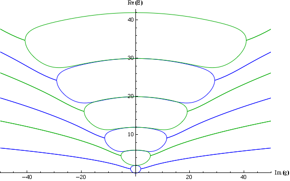
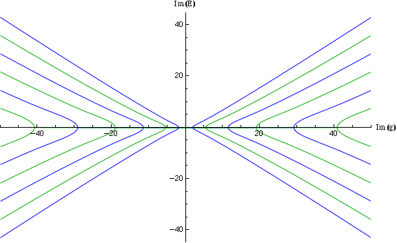
Figure 1: Real and imaginary components of eigenvalues $E$ for the Hamiltonian given by Eq.17. The first six eigenvalues for $m=0$ (blue) and $m=1$ (green) are shown. Intercepts on the $E$ axis are given by $\ell(\ell+1)$ for $\ell=0\;{\rm to}\;6$. For the case of $m=0$, we find that the spectrum is entirely real for $0\leq g<1.899$ at which point there is a transition to one pair of complex conjugate eigenvalues in the spectrum. At $g=11.45$ there is a second transition, to two pairs of complex conjugate eigenvalues. Similarly for the case of $m=1$, we find one complex conjugate eigenvalue pair at $g=5.41$, and two pairs at $g=19.04$. In these computations the Hamiltonian is truncated to a 100$\times$100 matrix; we have verified that the relevant part of the spectrum is insensitive to the truncation.

Let us choose basis elements

$$|l\rangle\rightarrow N_{l}P_{l,|m|}(\eta)$$ (18)

where $l=|m|,|m|+1,\ldots$, $P_{l,|m|}$ are the associated Legendre polynomials, with conventional normalization factor

$$N_{l}=\sqrt{\frac{(2l+1)}{2}}\sqrt{\frac{(l-|m|)!}{(l+|m|)!}}.$$ (19)

The $P_{l,m}$’s satisfy

$$h_{0}P_{l,|m|}(\eta)=l(l+1)P_{l,|m|}(\eta)$$ (20)

so the matrix of $h_{0}$ in this basis is diagonal. The matrix elements of the potential term, $ig\eta$, can easily be determined from the normalization and recursion relations of the $P_{l,m}$’s. By diagonalizing the truncated Hamiltonian matrix we can numerically obtain the eigenvalues of eq (17); see Fig. (1).

3 ${\cal PT}$ Vector Model in Finite-Dimensional Hilbert Space

$E3$ may also be regarded as a realization of the ${\cal PT}$ vector model with symmetry group $SO(3)$ and for which the Hilbert space is infinite dimensional. Now we wish to turn out attention to realizations of the ${\cal PT}$ vector model with finite dimensional Hilbert spaces. Let us write a simple, generic Hamiltonian $H=H_{0}+H_{I}$ where

$$H_{0}=L_{x}^{2}+L_{y}^{2}+L_{z}^{2}$$ (21)

$$H_{I}=V_{z}$$ (22)

and $V_{z}$ is the $z$ component of a vector operator.

Our task is to obtain a matrix representation of the total Hamiltonian, solve for its eigenvalues and determine what value of the non-Hermitian perturbation cause the eigenvalues to become complex.

Naturally we choose to work with the angular momentum eigenstates $|\ell,m\rangle$; the action of $H_{0}$ on these states is well known, and we can utilize the Wigner-Eckart theorem to determine the action of $H_{I}=V_{z}$.

Note that the dimensionality of the relevant vector space depends on the angular momenta of the multiplets but clearly it is finite. Suppose we consider the two multiplets $|\ell,m\rangle$ and $|\ell+1,m\rangle$; $m$ takes on values from $-\ell$ to $+\ell$ in the first multiplet and from $-\ell-1$ to $\ell+1$ in the second multiplet, so there are $(2\ell+1)+(2\ell+3)=4\ell+4$ of these states.

The action of $H_{0}$ on these states is simply

$$L^{2}|\ell,m\rangle=\ell(\ell+1)|\ell,m\rangle$$ (23)

$$L^{2}|\ell+1,m\rangle=(\ell+1)(\ell+2)|\ell+1,m\rangle.$$ (24)

So all that remains is to determine how $V_{z}$ acts on these states; here we employ the Wigner-Eckart theorem, which we have extended to the non-Hermitian case as detailed in Appendix A. We find $\langle\ell^{\prime},m^{\prime}|V_{z}|\ell,m\rangle=0$ unless $m=m^{\prime}$. Thus we need only to determine

$$\langle\ell,m|V_{z}|\ell,m\rangle,$$

$$\langle\ell+1,m|V_{z}|\ell+1,m\rangle,$$

$$\langle\ell,m|V_{z}|\ell+1,m\rangle,\;{\rm and}$$

$$\langle\ell+1,m|V_{z}|\ell,m\rangle$$

in order to completely specify $V_{z}$ in this space. The first two in this list can be expressed in terms of the reduced matrix element $\alpha$ defined in Appendix A; in general we find

$$\langle\ell,m|V_{z}|\ell,m\rangle =m\alpha_{1}$$

$$\langle\ell+1,m|V_{z}|\ell+1,m\rangle =m\alpha_{2};$$

however we also wish to enforce ${\cal P}V_{z}{\cal P}=-V_{z}$ and ${\cal T}V_{z}{\cal T}=-V_{z}$, which restricts $\alpha_{1}=\alpha_{2}=0$. (Determination of ${\cal P}$ and ${\cal T}$ within this space follows straightforwardly from their action on the spherical harmonics $PY_{\ell m}(\theta,\phi)=(-1)^{\ell}Y_{\ell m}(\theta,\phi)$ and $TY_{\ell m}(\theta,\phi)=Y^{\ast}_{\ell m}(\theta,\phi)=(-1)^{m}Y_{\ell,-m}(\theta,\phi)$.)

For the other two types of matrix elements, $\langle\ell,m|V_{z}|\ell+1,m\rangle$ and$\langle\ell+1,m|V_{z}|\ell,m\rangle$, we find these are proportional to other reduced matrix elements $\beta$ and $\gamma$;

$$\langle\ell+1,m|V_{z}|\ell,m\rangle =f_{\ell m}\beta,$$

$$\langle\ell,m|V_{z}|\ell+1,m\rangle =f_{\ell m}\gamma$$

where

$$f_{lm}=\left[\frac{(\ell+1)^{2}-m^{2}}{(2\ell+1)(2\ell+2)}\right]^{1/2}.$$ (25)

Note that $f_{\ell m}$ is even in $m$. When we enforce $PV_{z}P=-V_{z}$ and $TV_{z}T=-V_{z}$, we find this requires $\beta$ and $\gamma$ to be pure imaginary, so we define $\beta=ib$, $\gamma=ic$ for some real numbers $b,c$. Note that in determining these matrix elements we do not assume $V$ is Hermitian; we rely only on the commutators of $V$ with the angular momentum operators. (See Appendix A for details.)

Now let us write down the matrix corresponding to the Hamiltonian $H=H_{0}+H_{I}$. Consider the two-dimensional subspace spanned by the states $|\ell,m\rangle$ and $|\ell+1,m\rangle$ for a fixed value of $m$ that lies in the range $-\ell,\ldots,\ell$. Within this subspace

$$H_{0}=\left(\begin{array}[]{cc}\ell(\ell+1)&0\\ 0&(\ell+1)(\ell+2)\\ \end{array}\right)$$ (26)

and

$$V_{z}=\left(\begin{array}[]{cc}0&-icf_{\ell m}\\ -ibf_{\ell m}&0\\ \end{array}\right).$$ (27)

In addition consider the two dimensional subspace spanned by the states $|\ell+1,\ell+1\rangle$ and $|\ell+1,-\ell-1\rangle$. These states are not coupled by the perturbation $V_{z}$ to any other state and hence $V_{z}=0$ within this subspace. On the other hand the unperturbed Hamiltonian in this subspace is given by

$$H_{0}=\left(\begin{array}[]{cc}(\ell+1)(\ell+2)&0\\ 0&(\ell+1)(\ell+2)\\ \end{array}\right).$$ (28)

It is convenient to define

$$h_{\ell+1}=\left(\begin{array}[]{cc}(\ell+1)(\ell+2)&0\\ 0&(\ell+1)(\ell+2)\end{array}\right)$$ (29)

and

$$h_{m}=\left(\begin{array}[]{cc}\ell(\ell+1)&-icf_{lm}\\ -ibf_{lm}&(\ell+1)(\ell+2)\end{array}\right)$$ (30)

where $m=-\ell,\ldots,\ell$. The Hamiltonian can now be written as a block-diagonal matrix

$$\left(\begin{array}[]{ccccc}h_{\ell+1}&&&&\\ &h_{\ell}&&&\\ &&h_{\ell-1}&&\\ &&&\rotatebox{-35.0}{\huge{...}}&\\ &&&&h_{-\ell}\end{array}\right).$$ (31)

The individual $2\times 2$ matrices that constitute the Hamiltonian are simple enough that we can obtain analytic expressions for the eigenvalues. The eigenvalues of $h_{\ell+1}$ are two-fold degenerate and are simply $(\ell+1)(\ell+2)$. The eigenvalues of $h_{m}$ are

$$\lambda_{\ell m}^{\pm}=(\ell+1)^{2}\pm\sqrt{(\ell+1)^{2}-bcf_{\ell m}^{2}}$$ (32)

Note that $\lambda_{\ell,m}=\lambda_{\ell,-m}$ so for all $m\neq 0$ the eigenvalues of $h_{m}$ are also two-fold degenerate. Clearly, the eigenvalues are real provided

$$bc<\frac{(\ell+1)^{2}}{f_{lm}^{2}}.$$ (33)

We can make the following observations about the behavior of the eigenvalues. Once ${\cal PT}$ symmetry is broken, $\lambda^{+}$ and $\lambda^{-}$ form a complex conjugate pair. Since $f_{\ell m}$ has its maximum value for $m=0$, $\lambda^{\pm}$ becomes complex for $m=0$ first. Similarly, $f_{\ell m}$ is minimal for $|m|=\ell$, so $\lambda^{\pm}$ so these are the last eigenvalues to go complex. For example we consider the case $\ell=1$ and choose $b=c$ for simplicity. We plot the eigenvalues in Figure 2.

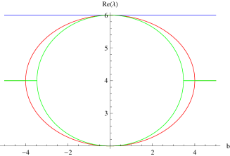
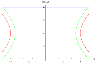
Figure 2: Real and imaginary parts of the eigenvalues $\lambda_{1,m}$ assuming $b=c$. The blue line at $\lambda=6$ corresponds to the $2\times 2$ matrix denoted $h_{\ell+1}$ in the text, with eigenvalues $(\ell+1)(\ell+2)$. The other eigenvalues are $m$-dependent and correspond to the $2\times 2$ matrices denoted $h_{m}$ in the text, with eigenvalues given by eq(32). As noted $\lambda_{\ell,m}=\lambda_{\ell,-m}$, so there are only two distinct $m$-dependent curves for $\ell=1$. In each figure, $|m|=1$ is plotted in red and $m=0$ is plotted in green. Note that the transition to complex eigenvalues occurs at $b=4$ for $\lambda^{\pm}_{1,1}$ and $b=\sqrt{12}\approx 3.47$ for $\lambda^{\pm}_{1,0}$.

It is worth noting that in the Hermitian case $b=-c$. Hence the condition in eq (33) that ensures the eigenvalues are real is always met.

4 Conclusion

We conclude by noting two natural generalizations of our results that deserve further investigation. First the model of a particle on an ordinary 2-sphere considered in section II may be generalized to a particle on a sphere in $n$ dimensions. The ${\cal PT}$ transition for this model may be amenable to analytic study in the large $n$ limit and may shed some light on ${\cal PT}$ symmetric non-linear sigma models of which it would represent a $0+1$ dimensional case Coleman:1974jh . Second the vector model constructed in section III may be easily generalized from the symmetry group SO(3) to any Lie group and therefore represents only one member of a large class of such models.

Appendix A: Wigner-Eckart Theorem

Suppose we have an angular momentum operator ${\mathbf{L}}$ and a vector operator ${\mathbf{V}}$ satisfying the commutation relations

$$[L_{i},V_{j}]=i\epsilon_{ijk}V_{k}.$$ (34)

Let $|\ell,m\rangle$ denote an angular momentum multiplet of total angular momentum $\ell$ and $z$-component $m$. Then according to the Wigner-Eckart theorem the matrix elements of $V_{z}$ and $V_{\pm}=V_{x}\pm iV_{y}$ between multiplet states are determined by the commutation relations eq (34). In the usual Wigner-Eckart theorem the Cartesian components of the operator ${\mathbf{V}}$ are assumed to be hermitian. Here we present a non-Hermitian generalization of the theorem.

Following the usual arguments we find the selection rules

$$\langle\ell^{\prime},m^{\prime}|V_{z}|\ell,m\rangle =0\;\;\;\;\;\;{\rm unless}\;m^{\prime}=m$$ (35)

$$\langle\ell^{\prime},m^{\prime}|V_{+}|\ell,m\rangle =0\;\;\;\;\;\;{\rm unless}\;m^{\prime}=m+1$$ (36)

$$\langle\ell^{\prime},m^{\prime}|V_{-}|\ell,m\rangle =0\;\;\;\;\;\;{\rm unless}\;m^{\prime}=m-1.$$ (37)

Furthermore the matrix elements vanish unless $\ell^{\prime}=\ell-1$ or $\ell^{\prime}=\ell$ or $\ell^{\prime}=\ell+1$.

Consider the case $\ell^{\prime}=\ell$. Generalization of the usual arguments shows that

$$\langle\ell,m+1|V_{+}|\ell,m\rangle = A(\ell-m)^{1/2}(\ell+m+1)^{1/2}\hskip 14.22636ptm=-\ell,\ldots,\ell-1$$

$$\langle\ell,m|V_{z}|\ell,m\rangle = Am\hskip 122.34685ptm=-\ell,\ldots,\ell$$

$$\langle\ell,m-1|V_{-}|\ell,m\rangle = A(\ell-m+1)^{1/2}(\ell+m)^{1/2}\hskip 14.22636ptm=-\ell+1,\ldots,\ell$$

where the proportionality constant $A$ is a complex number called the “reduced matrix element”. Note that for ${\mathbf{V}}$ hermitian, $A$ would have to be real, but there is no such restriction in the non-hermitian case.

Similarly in the case $\ell^{\prime}=\ell+1$ we find

$$\langle\ell+1,m+1|V_{+}|\ell,m\rangle = B\left[\frac{(\ell+m+2)(\ell+m+1)}{(2\ell+2)(2\ell+1)}\right]^{1/2}$$

$$\langle\ell+1,m|V_{z}|\ell,m\rangle = -B\left[\frac{(\ell-m+1)(\ell+m+1)}{(2\ell+2)(2\ell+1)}\right]^{1/2}$$

$$\langle\ell+1,m-1|V_{-}|\ell,m\rangle = -B\left[\frac{(\ell-m+1)(\ell-m+2)}{(2\ell+2)(2\ell+1)}\right]^{1/2},$$

where $m=-\ell,\ldots,\ell$ and $B$ is another complex reduced matrix element.

Finally in the case that $\ell^{\prime}=\ell-1$ we find

$$\langle\ell-1,m+1|V_{+}|\ell,m\rangle = -C\left[\frac{(\ell-m-1)(\ell-m)}{(2\ell)(2\ell-1)}\right]^{1/2}$$

$$\langle\ell-1,m|V_{z}|\ell,m\rangle = -C\left[\frac{(\ell-m)(\ell+m)}{(2\ell)(2\ell-1)}\right]^{1/2}$$

$$\langle\ell-1,m-1|V_{-}|\ell,m\rangle = C\left[\frac{(\ell+m)(\ell+m-1)}{(2\ell)(2\ell-1)}\right]^{1/2},$$ (40)

where $C$ is a complex reduced matrix element and $m=-\ell,\ldots,\ell-2$ in the first line of eq (40), $m=-\ell+1,\ldots,\ell-1$ in the second line of eq (40), and $m=-\ell+2,\ldots,\ell$ in the last line of eq (40).

In the hermitian case the reduced matrix elements satisfy $B=C^{\ast}$ but in the non-hermitian case there is no such restriction on the complex elements $B$ and $C$.

References

- (1) Bender, Carl M. and Boettcher, Stefan. “Real spectra in nonHermitian Hamiltonians having PT symmetry”, Phys. Rev. Lett. 80,5243-5246 (1998).
- (2) Bender, Carl M. and Boettcher, Stefan and Meisinger, Peter. “PT symmetric quantum mechanics”, J.Math.Phys 40, 2201-2229. (1999).
- (3) Bender, Carl M.,“Making sense of non-Hermitian Hamiltonians”,Rept.Prog.Phys., 70, 947. (2007).
- (4) Guo, A. and Salamo, G. J. and Duchesne, D. and Morandotti, R. and Volatier-Ravat, M. and Aimez, V. and Siviloglou, G. A. and Christodoulides, D. N. “Observation of -Symmetry Breaking in Complex Optical Potentials”, Phys. Rev. Lett. 103,093902 (2009).
- (5) Ruter, Christian E. and Makris, Konstantinos G. and El-Ganainy, Ramy and Christodoulides, Demetrios N. and Segev, Mordechai and Kip, Detlef. “Observation of parity-time symmetry in optics”, Nat. Phys. 6 1515. (2010).
- (6) Zhao, K. F. and Schaden, M. and Wu, Z. “Enhanced magnetic resonance signal of spin-polarized Rb atoms near surfaces of coated cells”,Phys. Rev. A, 81, 042903 (2010).
- (7) Bender, Carl and Kalveks, R.“” Symmetry from Heisenberg Algebra to E2 Algebra”, Int. J. Theo. Phys,50, 955-962, (2011).
- (8) Coleman, S. , R. Jackiw and H.D. Politzer, Phys. Rev. D10, 2491 (1974).