Generalized cable theory for neurons in complex and heterogeneous media

Abstract

Cable theory has been developed over the last decades, usually assuming that the extracellular space around membranes is a perfect resistor. However, extracellular media may display more complex electrical properties due to various phenomena, such as polarization, ionic diffusion or capacitive effects, but their impact on cable properties is not known. In this paper, we generalize cable theory for membranes embedded in arbitrarily complex extracellular media. We outline the generalized cable equations, then consider specific cases. The simplest case is a resistive medium, in which case the equations recover the traditional cable equations. We show that for more complex media, for example in the presence of ionic diffusion, the impact on cable properties such as voltage attenuation can be significant. We illustrate this numerically always by comparing the generalized cable to the traditional cable. We conclude that the nature of intracellular and extracellular media may have a strong influence on cable filtering as well as on the passive integrative properties of neurons.

I Introduction

Cable theory, initially developed by Rall Rall1962 , is one of the most significant contributions of theoretical neuroscience and has been extremely useful to explain a large range of phenomena (reviewed in Rall1995 ). However, cable theory makes a number of assumptions, one of which is that the extracellular space around neurons can be modeled by a resistance, or in other words, that the medium around neurons is resistive or ohmic. While some measurements seem to confirm this assumption Logothetis , other measurements revealed a marked frequency dependence of the extracellular resistivity Gabriel1996a ; Gabriel1996b , which indicates that the medium is non-resistive. Indirect measurements of the extracellular impedance also show evidence for deviations from resistivity BedDes2006a ; BedDes2010 ; Deg2010 ; Baz2011 , which could be explained by the influence of ionic diffusion BedDes2011a . Despite such evidence for non-resistive media, the possible impact on cable properties has not been evaluated.

The effect of non-resistive media can be investigated by integrating this effect in the impedance of the extracellular medium, $Z_{e}$, and in particular, through its frequency dependence. For example, it can be shown that $Z_{e}\sim 1/\omega$ for capacitive effects or electric polarization BedDes2006b , $Z_{e}\sim 1/\sqrt{\omega}$ for ionic diffusion (also called the “Warburg impedance” BedDes2009 ), while $Z_{e}$ would be constant for a perfectly resistive medium. To integrate such effects in a given formalism, such as the genesis of extracellular potentials, our approach has been to integrate a general frequency-dependent function $Z_{e}(\omega)$ in the formalism, and then consider specific cases BedDes2009 ; BedDes2011a .

In the present paper, we follow this approach and generalize cable equations for media with arbitrarily complex frequency-dependent impedance. With numerical simulations, we consider specific cases such as resistive media, ionic diffusion, capacitive media, etc. We evaluate a number of possible consequences on the variation of the membrane potential along the cable, and how such effects could be measured experimentally.

II Methods

All simulations were done using MATLAB. To simulate the cable structure of the models, a classic compartmental model strategy was used for simulations (see Fig. 3F), but was different from the one used in common simulator programs such as NEURON (Hines and Carnevale, Hines97 ). Each cylindric compartment is connected to intracellular and extracellular resistances or impedances, and these are normally used to solve the cable equations. In the present paper, we used another, equivalent method which consists of defining an auxiliary impedance, given by $Z_{a}=\frac{V_{m}}{i_{i}}$ where $V_{m}$ and $i_{i}$ are respectively the transmembrane potential and the axial current per unit length at the point where $Z_{a}$ is connected (see Fig. 1). This auxiliary impedance allows to take into account the influence of other compartments, including the soma, over the axial current and transmembrane potential. It is mathematically equivalent to consider the continuity conditions on axial current and transmembrane potential.

The electric and geometric parameters are considered constant in each compartment, but are allowed to vary between compartments. In these conditions, $V_{m}$ and $i_{i}$ are solution of partial differential equations (cable equations) and thus depend on spatial coordinates.

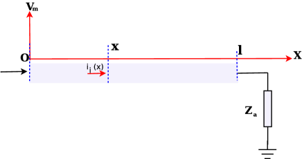
Figure 1: (Color online) Convention used to calculate the input impedance and transfer function. A cable segment of length $l$ is represented, with an impedance $Z_{a}$ in series, at the end of the cable. This “auxiliary impedance” $Z_{a}$ takes into account the influence of the other compartments on the axial current $i_{i}$ and transmembrane potential $V_{m}$ in a compact form. $Z_{a}=\frac{V_{m}(l)}{i_{i}(l)}$ where $i_{i}(l)$ is the current per unit length and $V_{m}(l)$ is the transmembrane voltage at coordinate $x=l$.

The cable equations simulated in this article are generalized to allow one to include media with complex electrical properties. We have designed a MATLAB code that simulates such generalized cable structures, using different types of linear density of complex impedances ($[\Omega/m]$) and specific impedances ($[\Omega.m]$) in each compartment. See Results for details of this method.

All computations were made in Fourier space. We have applied the theory to four different types of media to evidence their effect on the spatial and frequency profile of the membrane potential. These models are called SC, FC, FO and NIC, respectively (see Table 1). The SC model is the “standard model” as defined by Tuckwell Tuckwell ; the FC model corresponds to a model similar to the standard model (based on a closed circuit), but the cytoplasm and extracellular media impedances can be frequency-dependent. The FO type model is the same, with an open circuit (no return current). The NIC model includes a non-ideal capacitance similar to a previous study BedDes2008 . See Results for details of these models.

All numerical simulations were made using a “continuous ball-and-stick” model, consisting of a single cylindric compartment, described as a continuum (see Results), and a spherical soma. The dendritic compartment has a radius of $2~{}\mu m$ and a membrane time constant of $5~{}ms$, which corresponds to typical values of in vivo conditions. The has a radius of $7.5~{}nm$ and the specific capacitance was of $0.01~{}F/m^{2}$. These parameters represent typical values used in a number of previous studies Rall1995 ; Koch ; Wu ; Tuckwell .

$Types$	$Model$	$z_{e}^{(m)}$	$\lambda^{2}$	$\kappa_{\lambda}^{2}=\frac{1+i\omega\tau_{m}}{\lambda^{2}}$
SC	Standard cable	$z_{e}^{(m)}=-\frac{r_{m}r_{e}}{(r_{i}+r_{e})(1+i\omega\tau_{m})}$	$\frac{r_{m}}{r_{i}+r_{e}}$	$\frac{(r_{i}+r_{e})(1+i\omega\tau_{m})}{r_{m}}$
	(closed-circuit)
FC	Frequency-dependent cable	$z_{e}^{(m)}=-\frac{r_{m}z_{e}}{(z_{i}+z_{e})(1+i\omega\tau_{m})}$	$\frac{r_{m}}{z_{i}+z_{e}}$	$\frac{(z_{i}+z_{e})(1+i\omega\tau_{m})}{r_{m}}$
	(closed-circuit)
FO	Frequency-dependent cable	$z_{e}^{(m)}$	$\frac{r_{m}}{z_{i}}[1+\frac{z_{e}^{(m)}}{r_{m}}(1+i\omega\tau_{m})]$	$\frac{z_{i}(1+i\omega\tau_{m})}{r_{m}[1+\frac{z_{e}^{(m)}}{r_{m}}(1+i\omega\tau_{m})]}$
	(open-circuit)
NIC	Non-ideal cable	$z_{e}^{(m)}=-\frac{\omega^{2}r_{m}\tau_{m}\tau_{M}}{[1+i\omega(\tau_{m}+\tau_{M})][1+i\omega\tau_{m}]}$	$\frac{r_{m}}{z_{i}}[\frac{(1+i\omega\tau_{m})(1+i\omega\tau_{M})}{1+i\omega(\tau_{m}+\tau_{M})}]$	$\frac{z_{i}}{r_{m}}~{}[1+i\frac{\omega\tau_{m}}{1+i\omega\tau_{M}}]$
	(closed-circuit)

Table 1: Summary of dendritic cable types and parameters. The table gives the parameters $z_{e}^{(m)}$, $\lambda^{2}$ and $\kappa_{\lambda}$ for different model types. The standard model (SC) is the cable model as given by Rall, Koch and Tuckwell Rall1962 ; Koch ; Tuckwell . The “frequency-dependent model” (FC) correspond to a standard cable (closed circuit), but where the parameters $z_{i}$ and $z_{e}$ are allowed to be frequency dependent. In the “frequency-dependent open-circuit model” (FO), the current in the extracellular medium is “perpendicular” to the membrane (see Fig. 6). The “non-ideal cable” model (NIC) is similar to the standard model, but the capacitance of the membrane is non-ideal, as developed previously BedDes2008 . $z_{i}$ (see Eq. 10) and $z_{e}$ are respectively the impedance per unit length of the cytoplasm and of the extracellular medium, respectively, for FC type models. We write $r_{i}$ and $r_{e}$ when the parameters $z_{s}$ do not depend on frequency (SC type model). The parameter $z_{e}^{(m)}$ (see Eq. 18) is used in FO type models.

III Results

We start by generalizing the cable equations for membranes embedded within extracellular media of arbitrarily complex electrical properties. Next, we consider a few specific cases and numerical simulations.

III.1 Generalized cable equations

In this section, we redefine the cable equations taking into account the presence of complex and/or heterogeneous properties of extracellular and intracellular media. Because electrically complex or heterogeneous media can display charge accumulation, one cannot apply the usual (free-charge) current conservation law. One needs to use a more general conservation law based on the generalized current. In Section III.1.1 below, we derive this generalized current conservation law, while in Section III.1.2, we use this generalized conservation law to derive the generalized cable equations.

III.1.1 Generalized current conservation law in heterogeneous media

In this section, central to our theory, we show that the free-charge current conservation law ($\vec{j}^{~{}f}$) does not apply to systems with complex electrical properties. Another, more general, conservation law must be used, the generalized current conservation law. We derive here the conservation law for the membrane current in arbitrarily complex media, starting from first principles.

Maxwell theory of electromagnetism postulates that the following relation is always valid for any medium:

$$\nabla\times\vec{H}=\vec{j}^{~{}f}+\frac{\partial\vec{D}}{\partial t}~{},$$ (1)

where $\vec{H}$ is the magnetic field, and $\vec{j}^{~{}f}$ is the current density of free charges, and $\frac{\partial\vec{D}}{\partial t}$ is the displacement current density.

We define the generalized current density $\vec{j}^{~{}g}$ as:

$$\vec{j}^{~{}g}=\vec{j}^{~{}f}+\frac{\partial\vec{D}}{\partial t}=\vec{j}^{~{}f}+\vec{j}^{~{}d}~{},$$ (2)

where $\vec{j}^{~{}d}$ is the displacement current density.

It is important to note that the term $\frac{\partial\vec{D}}{\partial t}=\varepsilon_{o}\frac{\partial\vec{E}}{\partial t}$ is different from zero, even in the vacuum (assuming that the electric field varies in time).

The interest of using the generalized current, is that it is always conserved in any given volume, for any type of medium, as we explain below (see also Appendix A).

In the case of an electric field in a homogeneous and locally neutral medium, we have $\nabla\cdot\vec{j}^{~{}f}=-\frac{\partial\rho}{\partial t}^{f}=0$ because there cannot be charge accumulation anywhere. Because the relation $\nabla\cdot\vec{j}^{~{}g}=0$ applies to any type of medium, we also have $\nabla\cdot(\frac{\partial\vec{D}}{\partial t})=0$. Thus, in a homogeneous locally-neutral medium, we have two independent current conservation laws: one law applies to the free-charge current $i^{~{}f}$ and another one applies to the displacement current $i^{~{}d}$ . Note that in a homogeneous medium $i^{~{}d}$ is not necessarily negligible, but the application of the current conservation law on $i^{~{}f}$ can be done independently of the existence of $i^{~{}d}$ because the two laws are independent.

This is the framework assumed in the standard cable theory, in which the extracellular medium is resistive and homogeneous, the displacement current $i^{~{}d}$ is negligible, and there cannot be charge accumulation inside the dendrites nor in the extracellular medium. We will see below that these assumptions do not hold for complex extracellular media. If the medium is heterogeneous, then charge accumulation will necessarily appear in the presence of an applied electric field. Capacitive effects is an example of such charge accumulation. In such a case, the two current conservation laws on $i^{~{}f}$ and $i^{~{}d}$ do not apply to every region of space (see Appendix B). However, the generalized current conservation on $i^{~{}g}$ is still valid in all cases.

Thus, to derive cable equations in heterogeneous media, one must use the generalized current conservation law, as done in the next section.

III.1.2 Application of the generalized conservation law to cable equations

To start, we consider a small portion of membrane surface and build a domain in the intracellular side, which is limited by the interior surface of the membrane, while the other surfaces of the domain are located inside the cytoplasm (see Fig. 2).

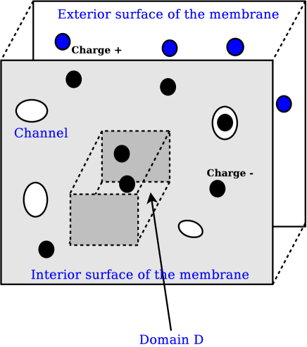
Figure 2: (Color online) Definition of a domain $\mathcal{D}$ inside the cytoplasm and adjacent to the membrane. Due to conductance variations in the membrane, or due to charged currents, the total charge in domain $\mathcal{D}$ varies. One cannot consider that the displacement current across the surface of domain $\mathcal{D}$ is zero, because this would be in contradiction with Maxwell-Gauss law (see Appendix B). Black circles represent negative charges on the interior surface of the membrane, as well as in the cytoplasm, while blue circles indicate positive charges at the exterior side of the membrane.

Using such a definition, in resting conditions, the intracellular side has an excess of negative charges, which are adjacent to the membrane. In such a state, we can calculate the free charge density in this domain from Maxwell-Gauss law:

$$Q(t)=\oiint\limits_{\partial\mathcal{D}}\vec{D}\cdot\hat{n}~{}dS=cst~{},$$ (3)

where $\partial\mathcal{D}$ is the surface of the considered domain

Now, suppose that a conductance variation occurs in the domain (for example following the opening of an ion channel). This will induce a charged current in domain $\mathcal{D}$ and therefore, there will be a variation of the total charge included within domain $\mathcal{D}$, which implies a non-zero displacement current $i^{~{}d}$ across the surface $\partial\mathcal{D}$ surrounding domain $\mathcal{D}$ (without this current, the system would be in contradiction with Maxwell-Gauss law; see Appendix B).

In such conditions, we have:

$$i^{~{}d}=\frac{dQ}{dt}=\oiint\limits_{\partial\mathcal{D}}\frac{\partial\vec{D}}{\partial t}\cdot\hat{n}~{}dS\neq 0$$ (4)

Can we neglect this current to study the variations of the membrane potential along the cable? Because it is difficult to give a rigorous answer to this question DesBed2012 ; Riera , in particular when $i^{~{}d}$ is non-zero, we consider the generalized current $i^{~{}g}$ because this current is conserved independently of $i^{~{}d}$ (see previous section). This will allow us to treat cable equations without making any hypothesis about charge accumulation inside or outside of the cable.

Moreover, to stay as general as possible, we include a frequency and space dependence of the electric parameters, which will allow us to simulate the effect of media of different electric properties, such as capacitive or diffusive BedDes2006b ; BedDes2009 ; BedDes2011a .

In this context, the linking equations must be expressed in their most general form BedDes2011a :

$$\left\{\begin{array}[]{ccc}\vec{D}(\vec{x},t)&=&\int_{-\infty}^{+\infty}\varepsilon_{i}(\vec{x},t-\tau)\vec{E}(x,\tau)~{}d\tau\\ \\ \vec{j}^{~{}f}(\vec{x},t)&=&\int_{-\infty}^{+\infty}[\sigma_{i}^{e}(\vec{x},t-\tau)\vec{E}(\vec{x},\tau)\end{array}\right.$$ (5)

According to this scheme, the generalized current density $\vec{j}_{i}^{~{}g}$ inside the cytoplasm obeys:

$$\vec{j}_{i}^{~{}g}(\vec{x},t)=\int_{-\infty}^{+\infty}[\sigma_{i}^{e}(\vec{x},t-\tau)\vec{E}(\vec{x},\tau)+\varepsilon_{i}(\vec{x},t-\tau)\frac{\partial\vec{E}}{\partial t}(\vec{x},\tau)]~{}d\tau$$ (6)

where $\sigma_{i}^{e}(\vec{x},t)$ is the intracellular electric conductivity function and $\varepsilon_{i}(\vec{x},t)$ is the intracellular electric permittivity function.

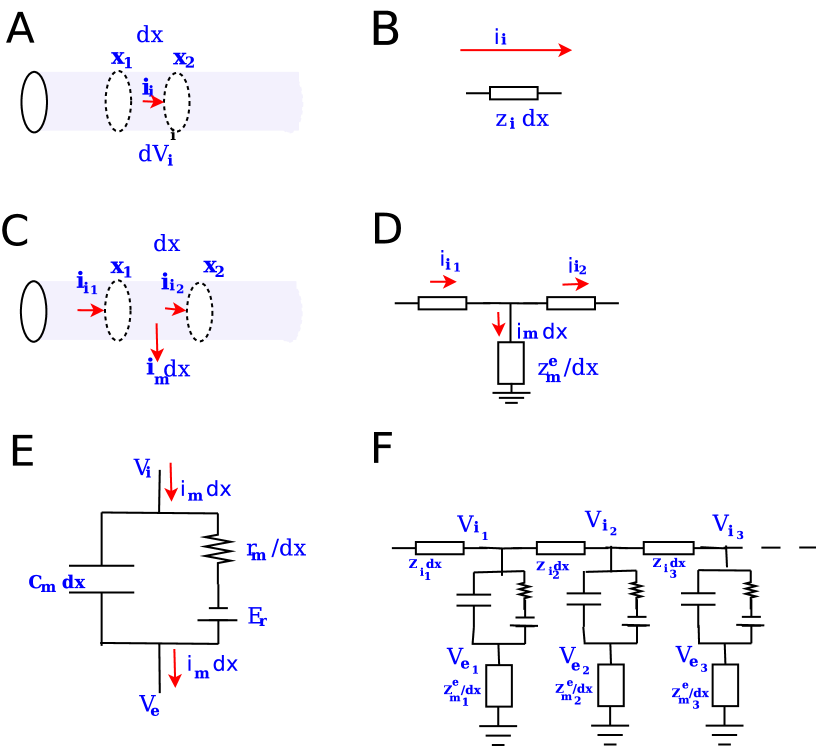
Figure 3: (Color online) Compartments and equivalent electrical circuits of the membrane and cable segments. $A$ and $C$ depict different configurations in a cable of constant diameter, with their respective equivalent electrical circuits shown in $B$ and $D$. $E$ is the equivalent electrical circuit of a membrane compartment of the cable, and $F$ is the equivalent circuit obtained for three compartments. $V_{i}$ is the intracellular potential relative to the reference, $V_{e}$ is the extracellular potential relative to the same reference, $z_{i}$ is the cytoplasm impedance, $r_{m}/dx$ and $z_{e}^{(m)}/dx$ are respectively the impedances of ion channels and the input impedance of the extracellular medium as seen by the transmembrane current. $i_{e}$ is the output current of a cable element in the extracellular medium, and $i_{i}$ is the axial current. The membrane potential $V_{m_{j}}$ equals $V_{i_{j}}-V_{e_{j}}$ and may vary according to the position $x_{j}$.

The first term in the integral accounts for energy dissipation phenomena, such as calorific dissipation (Ohm’s differential law) and diffusion phenomena. The second term represents the effect of charge density variations in the volume elements.

In Fourier frequency space, Eq. 6 becomes algebraic.

$$\vec{\j}_{i}^{~{}g}(\vec{x},\omega)=[\sigma_{i}^{e}(\vec{x},\omega)+i\omega\varepsilon_{i}(\vec{x},\omega)]\vec{E}(\vec{x},\omega)$$ (7)

Moreover, we have $\nabla\times\vec{E}=0$, which implies $\vec{E}=-\nabla V$ because electromagnetic induction is negligible in biological tissue (in the absence of magnetic stimulation).

If we now consider a one-dimensional cylindric cable of constant radius $a$ (Fig. 3A), the generalized current at a position $x$ of the cable can be written as:

$$i_{i}^{~{}g}(x,\omega)=\vec{j}_{i}^{~{}g}(x,\omega)\cdot(\pi a^{2}~{}\hat{n})=-\pi a^{2}[\sigma_{i}^{e}(x,\omega)+i\omega\varepsilon_{i}(x,\omega)]\cdot\frac{\partial V_{i}}{\partial x}(x,\omega)$$ (8)

where $V_{i}$ is the intracellular voltage difference with respect to a given reference (which can be far away). In the following of the text, we will call “compartment” a cylindric cable with constant radius and with uniform electric parameters (see Fig. 1). It is important to note that this compartment does not need to be isopotential, and the membrane potential will depend on the position on the compartment (see scheme in Fig. 1).

If we assume that the impedance (per unit length) of cytoplasm $z_{i}$ can be expressed as:

$$z_{i}=\frac{1}{\pi a^{2}[\sigma_{i}^{e}(x,\omega)+i\omega\varepsilon_{i}(x,\omega)]}~{},$$ (9)

then the axial current can be written as:

$$i_{i}^{~{}g}(x,\omega)=-\frac{1}{z_{i}}\frac{\partial V_{~{}i}}{\partial x}(x,\omega)$$ (10)

This expression is similar to the traditional cable equation Rall1995 ; Tuckwell ; Wu , with the exception that the parameter $z_{i}$ is complex (with units of $[\Omega/m]$). In addition, the transmembrane current $i_{m}^{\perp}$ over a cable length $dx$ can be expressed as:

$$i_{m}^{\perp}(x,t)=i_{m}~{}(x,t)~{}dx=2\pi adx~{}[~{}C_{m}\frac{\partial V_{m}(x,t)}{\partial t}+\frac{\sigma_{m}^{e}}{e}(V_{m}(x,t)-E_{m})~{}]=dx~{}[~{}c_{m}\frac{\partial V_{m}(x,t)}{\partial t}+\frac{(V_{m}(x,t)-E_{m})}{r_{m}}~{}]$$ (11)

where $V_{m}$ is the transmembrane voltage, $E_{m}$ is the resting membrane potential, $C_{m}$ is the specific membrane capacitance (in $F/m^{2}$), $c_{m}$ is the membrane capacitance per unit length (in $F/m$), $\sigma_{m}^{e}$ is the electric conductivity (in $S/m$), $1/r_{m}$ is the linear density of membrane conductance (in $S/m$), $e$ is the membrane thickness (in $m$) and $i_{m}$ is the transmembrane current per unit length (in $A/m$) (Figs 3C-E). Applying the inverse Fourier transform, we obtain:

$$\left\{\begin{array}[]{ccccc}i_{m}^{\perp}(x,0)&=&i_{m}~{}(x,0)~{}dx=~{}\frac{1}{r_{m}}[V_{m}(x,0)-2\pi E_{m}\delta(0)]~{}dx&&\omega=0\\ \\ i_{m}^{\perp}(x,\omega)&=&i_{m}~{}(x,\omega)~{}dx=~{}[i\omega c_{m}+\frac{1}{r_{m}}]V_{m}(x,\omega)~{}dx&&\omega\neq 0\end{array}\right.$$ (12)

Note that we assume here that the resting membrane potential $E_{m}$ does not depend on time nor on position in the cable.

Thus, we can see that the Fourier transform of Eq 10 generates a Dirac delta function for null frequency. In the following of the text, we consider frequencies different from zero, because the zero-frequency component of $i_{m}^{\perp}$ is zero for a signal of finite duration, which is always the case in reality.

In the model above, the expression of the transmembrane current is identical to the generalized membrane current for frequencies different from zero. In this case, the generalized current is given by:

$$i_{m}^{~{}g}=A\cdot j_{m}^{~{}g}=-2\pi a~{}dx(\sigma_{m}^{e}+i\omega\varepsilon_{m})\nabla V=2\pi a~{}dx(\sigma_{m}^{e}+i\omega\varepsilon_{m})\frac{V_{m}}{l}=dx~{}(\frac{1}{r_{m}}+i\omega c_{m})V_{m}=dx~{}i_{m}=i_{m}^{\perp}$$ (13)

where $l$ is the membrane thickness and $A$ is the membrane surface.

Assuming that the charge variations inside the channels is negligible, then the generalized current conservation law can apply to point B in the equivalent scheme (see Fig. 3 C), and we can write

$$i_{i}^{~{}g}(x+dx,\omega)=i_{i}^{~{}g}(x,\omega)-i_{m}^{~{}g}(x,\omega)=i_{i}^{~{}g}(x,\omega)-i_{m}^{\perp}(x,\omega)$$ (14)

It follows that:

$$di_{i}^{~{}g}(x,\omega)=\frac{\partial i_{i}^{~{}g}}{\partial x}~{}dx=-i_{m}^{\perp}(x,\omega)=-i_{m}~{}(x,\omega)~{}dx$$ (15)

Using Eqs. 6 and 11, we obtain:

$$\pi a^{2}\frac{\partial}{\partial x}[(\sigma_{i}^{e}(x,\omega)+i\omega\varepsilon_{i}(x,\omega))\frac{\partial V_{i}}{\partial x}(x,\omega)]=[i\omega c_{m}+\frac{1}{r_{m}}]V_{m}(x,\omega)$$

Applying the partial derivative on the lefthand term, and dividing by $\pi a^{2}(\sigma_{i}^{e}+i\omega\varepsilon_{i})$, one obtains:

$$\frac{\partial^{2}V_{i}}{\partial x^{2}}+\frac{1}{(\sigma_{i}^{e}+i\omega\varepsilon_{i})}\frac{\partial(\sigma_{i}^{e}+i\omega\varepsilon_{i})}{\partial x}\cdot\frac{\partial V_{i}}{\partial x}=\frac{1}{\pi a^{2}(\sigma_{i}^{e}+i\omega\varepsilon_{i})}[i\omega c_{m}+\frac{1}{r_{m}}]V_{m}=z_{i}i_{m}$$ (16)

Note that if the righthand term was zero, then this equation would be identical to the equation describing the electric potential outside of the sources BedDes2004 ; BedDes2009 ; BedDes2011a , because the $\nabla$ operator equals $\hat{e}_{x}\frac{\partial}{\partial x}$ in one dimension, in which case the right would be equal to $\nabla^{2}V_{i}+\frac{\nabla\gamma_{i}}{\gamma_{i}}\cdot\nabla V_{i}$ where $\gamma_{i}=\sigma_{i}^{e}+i\omega\varepsilon_{i}$.

We can simplify Eq. 14 if the cytoplasm is quasi-homogeneous (assuming the scale considered is large compared to inhomogeneities due to subcellular organelles), in which case we can consider that the electric parameters of the cytoplasm are independent of position x: $\sigma_{i}^{e}(x,\omega)=\sigma_{i}^{e}(\omega)$ and $\varepsilon_{i}(x,\omega)=\varepsilon_{i}(\omega)$. This leads to the following expression:

$$\frac{1}{z_{i}}\frac{\partial^{2}V_{~{}i}}{\partial x^{2}}(x,\omega)=\frac{1}{\pi a^{2}(\sigma_{i}^{e}+i\omega\varepsilon_{i})}\frac{\partial^{2}V_{~{}i}}{\partial x^{2}}(x,\omega)=[i\omega c_{m}+\frac{1}{r_{m}}]V_{m}(x,\omega)$$ (17)

in Fourier space.

If we now assume that the extracellular medium can also be considered as homogeneous (which will be valid at scales larger than the typical size of the cellular elements), then we can model the variations of the membrane potential caused by the transmembrane current $i_{m}^{\perp}$. We can model this effect from the notion of impedance, without making any hypothesis on the current field in the extracellular medium. In this case, one can associate to each cable segment $dx$ the specific impedance of the extracellular medium, $z_{e}^{(m)}$, as seen by the transmembrane current. $z_{e}^{(m)}$ has a similar physical meaning as $r_{m}$, except that it is a complex number in general. In Section III.2, we will see that $z_{e}^{(m)}$ depends on the direction of the current field in the extracellular medium.

Without any loss of generality, we can write in Fourier space:

$$V_{i}(x,\omega)=V_{m}(x,\omega)+z_{e}^{(m)}(\omega)i_{m}(x,\omega)~{}.$$ (18)

By substituting this last expression in Eq. 15, we obtain

$$\frac{r_{m}}{z_{i}}[1+\frac{z_{e}^{(m)}}{r_{m}}(1+i\omega\tau_{m})]~{}\frac{\partial^{2}V_{m}}{\partial x^{2}}=[1+i\omega\tau_{m}]V_{m}$$

where $\tau_{m}=r_{m}c_{m}$.

Thus, we can write the system in a form similar to the standard cable equation:

$$\lambda^{2}\frac{\partial^{2}V_{m}(x,\omega)}{\partial x^{2}}=\kappa^{2}V_{m}(x,\omega)$$ (19)

where

$$\left\{\begin{array}[]{ccc}\lambda^{2}&=&\frac{r_{m}}{z_{i}}\cdot[1+\frac{z_{e}^{(m)}}{r_{m}}(1+i\omega\tau_{m})]=\frac{r_{m}}{\bar{z}_{i}}\\ \\ \kappa^{2}&=&1+i\omega\tau_{m}\end{array}\right.$$ (20)

for a cylindric compartment (see Eq. 47 in Appendix C). It follows that the general solution of this equation in Fourier space $\omega\neq 0$ is given by:

$$V_{m}(x,\omega)=A^{+}(\omega)e^{\frac{\kappa(l-x)}{\lambda}}+A^{-}(\omega)e^{\frac{-\kappa(l-x)}{\lambda}}$$ (21)

for each cylindric compartment of length $l$ and with constant diameter (see Fig. 1 for a definition of coordinates). For a given frequency, we have a second order differential equation with constant coefficients.

In general, one can apply Eq. 21 for different cylindric compartments, as in Fig. 3F. In this case, one must adjust the different compartments to their specific limit conditions (continuity of $V_{m}$ and of the current $i_{i}^{~{}g}=-\frac{1}{\bar{z}_{i}}\frac{\partial V_{m}}{\partial x}$ (see Eq. 43 in Appendix C).

Note that Eq. 21 is exact for a cylindric compartment of constant diameter. Thus, it is possible to use this property to simulate exactly the full cylindric compartment as a continuum with no need of spatial discretization into segments, as usually done in numerical simulators. This is only possible if the cylindric compartment has a constant diameter. This leads to an efficient method to simulate the cable equations. We will refer to this approach as “continuous compartment” in the following.

As mentioned above, the mathematical forms of Eqs. 19 and 21 are identical to that of the standard cable model, but with different definitions of $\lambda$. Thus, we directly see that the nature of the extracellular medium will change the value of these parameters, which become frequency dependent. In particular, we see from Eq. 19 that changing these parameters will impact on the spatial profile of the variations of $V_{m}$, if the frequency dependence of the ratio $\kappa_{\lambda}=\frac{\kappa}{\lambda}$ is affected by the nature of the medium. Thus, experimental measurement of the spatial variations of $V_{m}$ will be able to identify effects of the extracellular impedance only if the ratio $\kappa_{\lambda}$ is affected.

In the next section, we derive expressions to calculate the input impedance $Z_{in}(P)=\frac{V_{m}(P,\omega)}{i_{i}(P,\omega)}$ and the transfer function of the transmembrane voltage $F_{T}(\omega)=\frac{V_{m}(P_{b},\omega)}{V_{m}(P_{a},\omega)}$ between two positions in the cable (as a function of the ratio $\kappa_{\lambda}$). Later in Section III.2, we will see that it is necessary to know these quantities to calculate the spatial variation of $V_{m}$ and compare the standard model with the cable model embedded into complex extracellular media.

III.1.3 Method to solve the generalized cable

In this section, we present the theoretical expressions which will allow us to calculate the input impedances needed for computing the membrane voltage on a cable with varying diameter. We consider the input impedance of the membrane, as well as the impedance of the extracellular medium, both of which are needed to calculate the spatial profile of the $V_{m}$ in a given cable segment.

We proceed according to the following steps:

1. In the previous section, we saw that it is necessary to calculate the ratio $Z_{in}(P)=\frac{V_{m}(P,\omega)}{i_{i}(P,\omega)}$ at the position of the current source, to calculate the $V_{m}$ produced at that point.

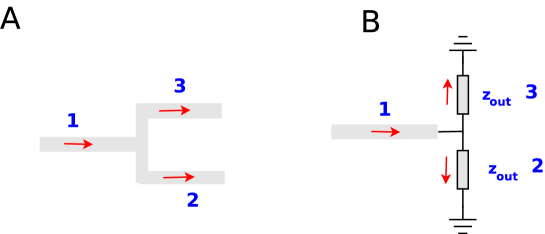
Figure 4: (Color online) Branching cables. The panels A and B respectively represent a branched cable where a dendrite separates into two daughter branches, and its equivalent electrical circuit. The equivalent impedance of segment 1 is equal to the input impedances of segments 2 and 3 ($z_{out~{}2}$ and $z_{out~{}3}$ ) taken in parallel.

One strategy is, in a first step, to separate the cable into a series of continuous compartments of constant diameter, where parameters $a$ (Eq. 8), $z_{i}$ (Eq. 10), $r_{m}$ (Eq. 11) and $z_{e}^{(m)}$ (Eq 18) are constant and specific to each compartment. In a second step, one calculates the (transmembrane) input impedance $Z_{in}^{n+1}=\frac{V_{m}(0)}{i_{i}(0)}$ at the begin of each compartment by taking into account the auxiliary impedance at the end of this compartment, $Z_{a}=Z_{out}^{n+1}=\frac{V_{m}(l_{n+1})}{i_{i}(l_{n+1})}=Z_{in}^{n}$ (see Fig. 1) if there is no branching point. At the branching points, the auxiliary impedances are simply equal to the equivalent input impedance of $n$ dendritic branches in parallel (where $n$ is the number of “daughter” branches; see Fig. 4). Thus, because the input impedance at one end is equal to the input impedance of the other compartment connected to this end, one obtains a recursive relation (see Eq. 48 in Appendix C):

$$Z_{in}^{n+1}[Z_{in}^{n}]=\frac{\bar{z}_{i_{n}}}{\kappa_{{\lambda}_{n}}}~{}\frac{(\kappa_{{\lambda}_{n}}Z_{in}^{n}+\bar{z}_{i_{n}})~{}e^{2\kappa_{{\lambda}_{n}}l_{n}}+(\kappa_{{\lambda}_{n}}Z_{in}^{n}-\bar{z}_{i_{n}})}{(\kappa_{{\lambda}_{n}}Z_{in}^{n}+\bar{z}_{i_{n}})~{}e^{2\kappa_{{\lambda}_{n}}l_{n}}-(\kappa_{{\lambda}_{n}}Z_{in}^{n}-\bar{z}_{i_{n}})}$$ (22)

where

$$\bar{z}_{i}=\frac{z_{i}}{1+\frac{z_{e}^{(m)}}{r_{m}}(1+i\omega\tau_{m})}$$

Thus, we can write

$$Z_{in}^{n+1}=F~{}[Z_{in}^{n}~{};~{}\bar{z}_{i_{n}},\kappa_{\lambda_{n}},l_{n}]$$

This leads to the following expression to relate the first to the $n^{th}$ segment:

$$Z_{in}^{n+1}=F~{}[...F~{}[F~{}[Z_{in}^{1}~{};~{}\bar{z}_{i_{1}},\kappa_{\lambda_{1}},l_{1}];~{}\bar{z}_{i_{2}},\kappa_{\lambda_{2}},l_{2}]...;~{}\bar{z}_{i_{n}},\kappa_{\lambda_{n}},l_{n}]$$ (23)

Note that this algorithm is a generalization of that used to calculate the equivalent resistance for resistances in series. Indeed, for resistance in series we have $r_{eq}=F(...F(r_{1};r_{2});r_{n})$ where $F(r_{a};r_{b})=r_{a}+r_{b}$. The difference between this recurrence function and that of Eq. 25 essentially comes from the fact that there is no current leak in a resistance, while there is one in a dendritic compartment.

2. To calculate the profile of $V_{m}$ along the cable, one must use the spatial transfer function $\frac{V_{m}(P_{n+1},\omega)}{V_{m}(P_{n},\omega)}$ on a continuous cylindric compartment of arbitrary length, and calculate the product of the transfer functions between each connected compartment. This leads to (see Appendix D and Eq. 51):

$$F_{T}(l,\omega;Z_{out}^{n})=\frac{\kappa_{\lambda}Z_{out}^{n}}{\kappa_{\lambda}Z_{out}^{n}~{}cosh(\kappa_{\lambda}l)+\bar{z}_{i}sinh(\kappa_{\lambda}l)}$$ (24)

$$\frac{V_{m}(P_{n},\omega)}{V_{m}(P_{1},\omega)}=\prod_{i=1}^{n-1}\frac{V_{m}(P_{i+1},\omega)}{V_{m}(P_{i},\omega)}$$ (25)

3. To evaluate $z_{proximal}$ we must calculate the first impedance $Z_{in}^{1}$ which enters the recursive relation 24. This impedance corresponds to the impedance of the soma, which is given by:

$$Z_{in}^{1}=Z_{s}+Z_{cs},$$ (26)

where $Z_{s}$ is the soma membrane impedance and $Z_{cs}$ is the cytoplasm impedance inside the soma. This relation is obtained under the hypothesis that the soma is isopotential, and the application of the generalized current conservation law implies $i^{~{}g}=\frac{V_{i}-V_{e}}{Z_{s}+Z_{cs}}\approx\frac{V_{m}}{Z_{s}+Z_{cs}}$ where $V_{i}$ and $V_{e}$ are the electric potentials at both sides of the membrane, inside and outside, respectively relative to a reference located far-away.

The impedance of the bilipidic membrane is approximated by a parallel RC circuit where $R=R_{m}$ is the resistance and $\tau_{m}=R_{m}C_{m}$ is the membrane time constant. Thus, $Z_{in}^{1}$ can be written as:

$$Z_{in}^{1}=Z_{s}+Z_{cs}=\frac{R_{m}}{1+i\omega\tau_{m}}+Z_{cs}$$ (27)

Finally, to evaluate $z_{distal}$, we use the “sealed end” boundary condition $Z_{in}^{1}=\infty$. In this condition, we have $Z_{in}^{2}=\frac{\bar{z}_{i_{1}}}{\kappa_{\lambda_{1}}}~{}coth(\kappa_{\lambda_{1}}l_{1})$ (see Eq. 22). In the case of a single dendritic branch, we can write:

$$Z_{in}^{distal}=\frac{\bar{z}_{i}}{\kappa_{\lambda}}~{}coth(\kappa_{\lambda}l)~{},$$ (28)

where $l$ is the total length of the cable.

In the next section, we turn to numerical simulations to investigate passive cable properties in the presence of complex media. We consider the most general case, where both the impedance of the extracellular medium and that of cytoplasm can be frequency dependent, and determine the respective impact on the spatial profile and frequency content of the transmembrane voltage at the level of the proximal and distal ends of the cable.

III.2 Numerical simulations

The goal of the numerical simulations is here to show how the physical nature of extracellular and intracellular media can influence the spatial and frequency profiles of the transmembrane potential. We present simulations of a “continuous ball and stick” model, which consists of a continuous cylindric compartment (described by Eq. 21), connected to a spherical soma. In this case, the impedance $Z_{a}$ of the continuous cylindric compartment is the soma impedance (see Fig. 1). We do not investigate here the effect of complex dendritic structures, which is left for future studies. Note that what we call a “continuous cylindric compartment” actually represents an infinite number of compartments each represented by a resistance in series with a parallel RC circuit (see Fig. 3F).

In a first step, we list the different types of models of intracellular and extracellular media that were used. In a second step, we present the results of numerical simulations.

III.2.1 Different types of cable models

We now explain the parameters used for the simulations of the cable presented in Section III.3.

Because the cable equation (Eq. 19) is completely determined by the value of $\kappa_{\lambda}$ for a given frequency, the spatial and frequency profiles of the transmembrane voltage are completely determined if the geometry and boundary conditions are set. And because $\kappa_{\lambda}$ is a function of 4 parameters ($r_{m},\tau_{m},z_{i},z_{e}^{(m)}$)(Eq. 20) for a given frequency, we have a four-dimensional parameter space where the two last parameters ($z_{i},z_{e}^{(m)}$) can be frequency dependent. We will limit our exploration of this parameter space by only varying the physical nature of these impedances for realistic values of $r_{m}$ and $\tau_{m}$, because the influence of these parameters has been largely characterized in previous studies Rall1962 ; Koch ; Wu . Furthermore, with $\tau_{m}$ and $\omega$ fixed, the relation $\kappa_{\lambda}=\frac{1+i\omega\tau_{m}}{\lambda}$ depends only on $\lambda$, and thus, like the classic studies on cable equations, we will use this parameter as a main determinant of the cable properties.

We will explore the generalized cable equations by considering several typical cases:

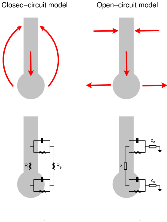
Figure 5: (Color online) Two different cable models for neurons. Left: Closed-circuit model. This is the standard cable model which forms a closed system (all inward and outward currents are balanced) and can be described by an equivalent circuit (bottom; shown here for a two-compartment model; $R_{e}$ and $R_{i}$ are the extracellular and intracellular resistances, respectively). In this model, the current flows parallel to the neuron. Right: Open-circuit model. In this more general model, the current is allowed to flow between neighboring neurons, or between the neuron and extracellular space, with no necessary condition of local balance (top). In this case, the neuron is modeled by an open circuit (bottom), and the current flows “perpendicular” to the membrane. The equivalent circuit is modeled more generally with impedances ($Z_{e}$ extracellular, $Z_{i}$ intracellular)

Standard cable model

The first type of model that we will consider is the “standard cable model” (model SC in Table 1), identical to that considered by Rall, Koch and Tuckwell Rall1962 ; Koch ; Tuckwell . In this model, the neuron is a closed system, where the inward and outward currents are balanced, forming a closed circuit (see Fig. 6, left). The extracellular current flows parallel to the dendrite, as noted previously Tuckwell . This model is equivalent to consider that the field produced by the neuron corresponds to an electric dipole configuration. In addition, this model considers that the extracellular medium is resistive, or in other words, that the extracellular impedance is a constant.

In this standard model, the extracellular impedance $z_{e}^{(m)}$ is either zero (no extracellular resistivity) as in Rall’s and Koch’s formulations Rall1962 ; Rall1995 ; Koch , or is equal to a constant, which is equivalent to model the extracellular medium by a resistance, as in other formulations Tuckwell ; Rieracable . Besides its physical non-sense (the extracellular medium considered as a supraconductor), using a zero-resistance is usually justified from the fact that the extracellular resistivity is much smaller than the membrane impedance. We will see that this justification does not hold if the medium is frequency dependent, in which case for some frequency range the extracellular resistivity may be determinant. Thus, to obtain the general expression of $\lambda$ and $\kappa_{\lambda}$ for the standard model, we set $z_{e}^{(m)}=-\frac{r_{m}r_{e}}{(r_{i}+r_{e})(1+i\omega\tau_{m})}$ in Eq. 20 (see Table 1).

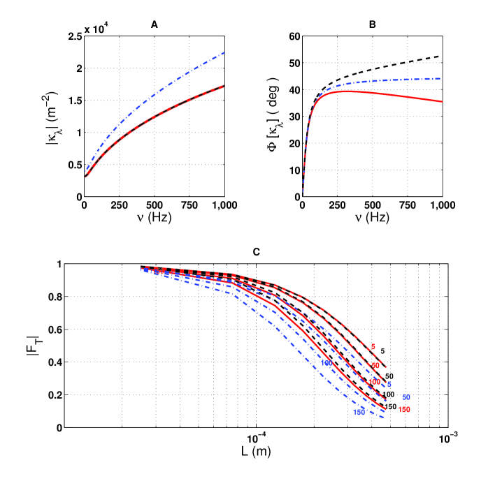
Figure 6: (Color online) Spatial and frequency profile of the membrane potential in the cable model with resistive media. A and B respectively show the modulus $|\kappa_{\lambda}|$ and the phase $\Phi[\kappa_{\lambda}]$ of $\kappa_{\lambda}$ as a function of frequency $\nu$ for a continuous ball-and-stick model. C. Modulus of the transfer function $|F_{T}|$ as a function of distance $L$ in the dendritic compartment, for frequencies equal to 5, 50, 100 and 150 Hz (see corresponding frequencies in A and B). The blue curves in $-\cdot-$ correspond to a standard cable model (FC, closed-circuit), with $r_{i}=28\times 10^{9}~{}\Omega/m$ and $r_{e}=18\times 10^{9}~{}\Omega/m$ . The red curves correspond to the same model but in an open-circuit configuration (FO model), with $r_{i}=28\times 10^{9}~{}\Omega/m$ and $z_{e}^{(m)}=0.01~{}\tau_{m}/2\pi aC_{m}=0.4\times 10^{3}~{}\Omega.m$. The black curves in $--$ show a non-ideal cable (NIC) model with $\tau_{M}=0.01\tau_{m}$, $r_{i}=28\times 10^{9}~{}\Omega/m$ and $r_{e}=0~{}\Omega/m$.

Frequency-dependent cable model

The second type of model is an extension of the standard model, where the intracellular and extracellular impedances ($z_{i}$ and $z_{e}^{(m)}$, respectively) are allowed to depend on frequency. This “frequency-dependent cable model” (model FC in Table 1) can account for example for a neuron embedded in capacitive or diffusive extracellular media, or if the intracellular medium has such properties, or both. In such cases, the appropriate frequency-dependent profiles for the impedances must be used.

In this frequency-dependent model, if $\tau_{m}$ is fixed, the quantity $z_{e}+z_{i}$ completely determines the spatial and frequency profiles of the V_m, and how they deviate from the standard model (see Table 1). To explore the effect of the impedances $z_{i}+z_{e}$, we consider three typical cases: “resistive”, “capacitive” (which is in fact resistive and capacitive in parallel) and “diffusive” (which is equivalent to a Warburg type impedance). Such impedances have also been considered in previous studies BedDes2010 ; BedDes2009 ; Poz .

Note that, in order to simulate the standard model, one must necessarily assume that the real part of $z_{e}^{(m)}$ is negative, which implies that $z_{e}^{(m)}$ is not a passive impedance per unit length, but is active, and thus requires a source of energy, as pointed previously Conciauro ; Mauro . This point will be further considered in the Discussion.

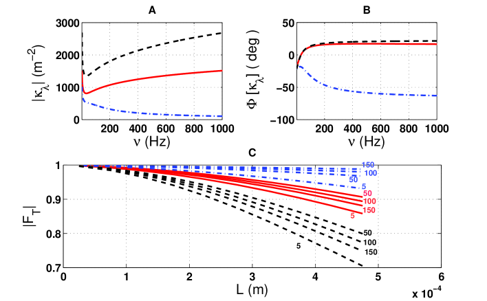
Figure 7: (Color online) Spatial and frequency profiles of the membrane potential for a model with resistive extracellular medium and diffusive cytoplasm. A and B: modulus $|\kappa_{\lambda}|$ and phase $\Phi[\kappa_{\lambda}]$ of $\kappa_{\lambda}$ as a function of frequency, for a continuous ball-and-stick model. C. Modulus of the transfer function $|F_{T}|$ as a function of distance for different frequencies (same arrangement as Fig. 6). The red curves correspond to a model with zero extracellular resistance. The blue curves ($-\cdot-$) show models with open-circuit configuration (FO model with $z_{e}^{(m)}=0.5~{}\tau_{m}/2\pi aC_{m}=20\times 10^{3}~{}\Omega.m$) and diffusive cytoplasm ($z_{i}=\frac{28\times 10^{9}}{(1+i)\sqrt{w}}~{}\Omega/m$). The black curves ($--$) show the same model with closed-circuit configuration with a resistive extracellular medium (FC model $r_{e}=18\times 10^{9}~{}\Omega/m$). Note that for the FC model, $|F_{T}|$ progressively increases from 5 to 50 Hz, then decreases between 50 and 100 Hz.

Open-circuit model

In a third type of model, the “Open-circuit” model (FO in Table 1), we use a different approach. Instead of considering the neuron as a closed system, where all outward currents must return to the neuron, we make no hypothesis about the return currents, and allow for example that neighboring neurons exchange currents. In this case, one does not need to describe each neuron by a closed circuit, but all neurons are open circuits are are connected together (through the extracellular space). Figure 6 shows the current fluxes of the two models, the standard model is a closed circuit where the outward currents loop into the inward currents (Fig. 6A), while in the open-circuit model, all currents are exchanged with the surrounding medium (Fig. 6B). These two models correspond to different equivalent circuits (Fig. 11 in Appendix E).

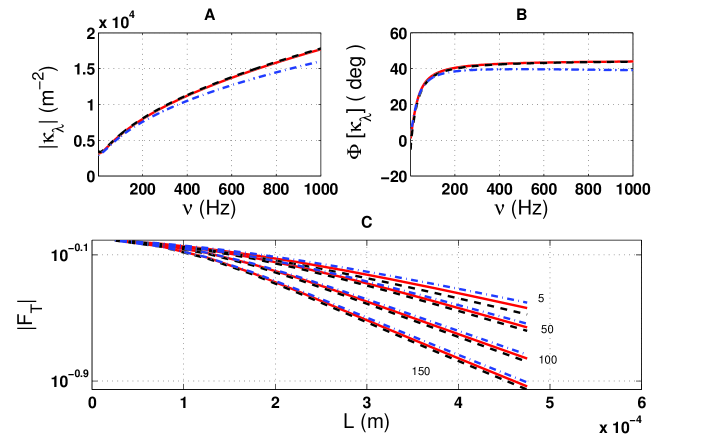
Figure 8: (Color online) Spatial and frequency profiles for a model with resistive cytoplasm and diffusive extracellular medium. Same arrangement of panels as for Figs. 6 and 7, but for different media. The black curves ($--$) show the behavior of a closed-circuit (FC) type model with resistive cytoplasm ($r_{i}=28\times 10^{9}~{}\Omega/m$) and diffusive extracellular space with Warburg impedance ($z_{e}=\frac{18\times 10^{9}}{(1+i)\sqrt{w}}~{}\Omega/m$). The red curves correspond to a closed-circuit (FC) type model with $z_{i}=28\times 10^{9}~{}\Omega/m$ and $z_{e}=0~{}\Omega/m$. The blue curves ($-\cdot-$) correspond to an open-circuit (FO) type model ($r_{i}=28\times 10^{9}~{}\Omega/m$, $z_{e}^{(m)}=\frac{\tau_{m}}{2\pi aC_{m}}\frac{0.5}{(1+i)\sqrt{w}}=\frac{20\times 10^{3}}{(1+i)\sqrt{w}}~{}\Omega.m$).

Note that the Open-circuit cable model is practically equivalent to the traditional (closed-circuit) cable model for an isolated neuron, if the impedance of the extracellular medium is negligible compared to the membrane impedance. Indeed, if $z_{e}^{(m)}$ and $z_{e}$ tend to $0$, then we have (see Table 1):

$$\lim_{{\color[rgb]{0,0,0.65}z_{e}^{(m)}}\rightarrow 0}\lambda_{FO}^{2}=\frac{r_{m}}{z_{i}}=\lim_{z_{e}\rightarrow 0}\lambda_{FC}^{2}$$ (29)

Similar to the frequency-dependent cable model, we will consider the three types of impedances discussed above (resistive, capacitive and diffusive) in the simulations of the Open-circuit model. In this case, we separately consider the two quantities $z_{i}$ and $z_{e}^{(m)}$ because these two parameters directly determine the value of $\lambda$ in models of FO type (see Table 1). Note that in the Open-circuit model, the real part of $z_{e}^{(m)}$ is always positive, so there is no need of any additional energy source (see Discussion).

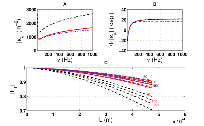
Figure 9: (Color online) Spatial and frequency profiles for fully diffusive cable models. Same arrangement of panels as for Figs. 6–8, but using a continuous ball-and-stick model where both cytoplasmic and extracellular impedances are of diffusive (Warburg) type. The black curves ($--$) correspond to a closed-circuit (FC) type model with $z_{i}=\frac{28\times 10^{9}}{(1+i)\sqrt{w}}~{}\Omega/m$ and $z_{e}=\frac{18\times 10^{9}}{(1+i)\sqrt{w}}~{}\Omega/m$. The red curves correspond to a closed-circuit (FC) type model with $z_{i}=\frac{28\times 10^{9}}{(1+i)\sqrt{w}}~{}\Omega/m$ and $z_{e}=0~{}\Omega/m$. The blue curves ($-\cdot-$) correspond to a closed-circuit (FO) type model with $z_{i}=\frac{28\times 10^{9}}{(1+i)\sqrt{w}}~{}\Omega/m$ and $z_{e}^{(m)}=\frac{20\times 10^{3}}{(1+i)\sqrt{w}}~{}\Omega.m$. Note that for both types of models (FO and FC), $|F_{T}|$ increases between 5 and 50 Hz, then decreases between 50 and 100 Hz.

Non-ideal cable model

The fourth type of model considered here is the “non-ideal cable model” introduced previously BedDes2008 . This model postulated that the membrane capacitance is non-ideal, through the use of an additional resistance at the arms of the capacitor; this resistance models the fact that there is some inertia time to charge movement (or equivalently, a friction). Such a non-ideal capacitance resulted in a shallower frequency scaling, that is a higher capacity of the dendritic tree to propagate high-frequency events BedDes2008 . Note that in this model, the extracellular medium is modeled as a resistance, so in this respect, the non-ideal cable model is equivalent to the standard model. Mathematically, the non-ideal cable appears through the use of $z_{e}^{(m)}$ (see Table 1), which can therefore be viewed as a particular case of an influence of the extracellular medium on cable properties. Indeed, the non-ideal cable can be shown to be equivalent to – or a particular case of – the open-circuit model, where the $V_{m}$ corresponds to $V_{i}$ with a far-away reference (see Appendix E). We keep this model here for comparison.

III.3 Simulation of the different models

In this section, we present the results of numerical simulations of the models presented in the previous section (see Methods). The goal of these simulations is not to be exhaustive in considering all possible combinations of models, but present a few typical configurations. The central question is whether the nature of the extracellular medium can have determinant impact on cable properties, and for what type of configuration or parameter values does it happen ?

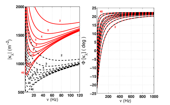
Figure 10: (Color online) Parameter $\kappa_{\lambda}$ as a function of frequency for fully diffusive models. The black curves $--$ correspond to FO and the red curves to FC type models with a time constant of $\tau_{m}=2,3,4,5,6,8,10,20$ and $40~{}ms$ . The FC type model was with $z_{i}=\frac{28\times 10^{9}}{(1+i)\sqrt{w}}~{}\Omega/m$ and $z_{e}=\frac{18\times 10^{9}}{(1+i)\sqrt{w}}~{}\Omega/m$ . For the FO type model, $z_{i}=\frac{28\times 10^{9}}{(1+i)\sqrt{w}}~{}\Omega/m$ and $z_{e}^{(m)}=\frac{\tau_{m}}{2\pi aC_{m}}\frac{0.5}{(1+i)\sqrt{w}}=\frac{20\times 10^{3}}{(1+i)\sqrt{w}}~{}\Omega.m$ (see Table 2 for the corresponding resonance frequencies).

Analysis of the spatial profiles of V_m variations

In this section, we investigate analytically and numerically different particular cases of extracellular and intracellular media to determine how the nature of these media affects the spatial and frequency profile of the membrane potential. We consider the transfer functions as defined in Table 1. The analyses presented here are limited to a ball-and-stick model, which allows a better interpretation of the effect of the physical nature of the different media. The effect of complex dendritic tree morphology will be the subject of a future study. To compare the results from the different models, we have considered models with identical geometry (see Methods for parameters).

Resistive models

We first considered the “standard model” with resistive intracellular and extracellular media, as well as the non-ideal cable model BedDes2008 . In Figure 7, we can see that the nature of the cable model (closed-circuit or open-circuit; non-ideal) influences the modulus and the phase of $\kappa_{\lambda}$, as well as the spatial profile of the transfer function $|F_{T}|$. The modulus of the transfer function depends more strongly on frequency in the FC model compared to the two other cases (Fig.7C), as observed previously BedDes2008 . Note that the parameters of the FO and NIC models were chosen such that they are equivalent (see Appendix B).

Capacitive models

Next, we considered models where the cytoplasm and extracellular medium are both of capacitive (RC-circuit) type. Note that we considered capacitive effects without ionic diffusion, because if both are combined, the resulting impedance is of Warburg type. This type of model will be considered next. With purely capacitive media, we observed effects very similar to the resistive model shown in Fig. 7, with slight differences only visible for large frequencies (greater than about $200~{}Hz$ (not shown). The small dimension of organelles ($<<1~{}\mu m^{2}$) within cells, as well as the distance between neighboring cells ($\sim 30~{}nm$ on average) Braitenberg ; Nicho2005 imply that the capacitance values of the media are necessary small compared to the membrane capacitance, and thus the purely capacitive effects (without diffusion) are likely to be negligible.

$\tau_{m}~{}(ms)$	$\nu_{r}~{}(Hz)$
2	83
3	54
4	40
5	30
6	25
8	20
10	18
20	8

Table 2: Resonance frequencies of fully diffusive models for different membrane time constants. The resonance frequencies of $|\kappa_{\lambda}|$ as a function of the membrane time constant $\tau_{m}$ (see Fig. 10).

Resistive models with diffusive cytoplasm

We next considered models where the extracellular medium was resistive as above, but where the intracellular medium (cytoplasm) was diffusive, and described by a Warburg impedance. Figure 7 shows the spatial and frequency behavior of this model. We can see that the open-circuit (FO) model shows less attenuation with distance compared to the closed-circuit (FC) model. Note that these two models give opposite variations when the extracellular medium has a zero resistance: in FC type models, $|F_{T}|$ attenuates more steeply as a function of distance when the extracellular impedance increases, whereas in FO type models, the attenuation becomes less steep. However, the spatial profile of $|F_{T}|$ also attenuates less with a diffusive cytoplasm compared to a resistive cytoplasm. The latter result is expected, because the higher the frequency the more the impedance “short-cuts” the membrane in this case. Note that the Warburg impedance used in all diffusive models considered here was applied for frequencies larger than $5~{}Hz$.

It is interesting to note that in the FC model, a resonance appears around 24 Hz in the modulus of the transfer function $\kappa_{\lambda}$ (Fig. 7A). In contrast, the FO model does not display a resonance.

Resistive cytoplasm with diffusive extracellular medium

Next, we considered the opposite configuration as previously, namely a resistive model for the cytoplasm, but a diffusive extracellular medium. Three sets of parameters were chosen for the extracellular space. First, a FO type model with a resistive cytoplasm and a diffusive extracellular medium described by a Warburg type impedance (black curve in Fig. 9), and second, a FC type model with similar parameters (blue curve in Fig. 8). These two models can be justified if one takes into account the Debye layer at the edge of the membrane Deg2010 ; BedDes2010 ; BedDes2011a ). The case with a zero extracellular resistance (short-cut) is also shown for comparison (red curve in Fig. 9). The latter model represents the same limit case for both FO and FC models, and therefore constitutes the frontier between the two families of curves.

Fully diffusive cable models

Next, we have considered the case where both intracellular and extracellular media are diffusive. Figure 9 shows the frequency and spatial profiles of the $V_{m}$ for such fully diffusive models. Taking the FO model with low extracellular impedance ($|z_{e}|=r_{e}$ at $1~{}Hz$) leads to large differences with the FC model (Fig. 9, black) compared to the FO model (blue) or the FC model with zero extracellular resistance (red).

We can see that, in FC type models, the larger $z_{e}$, the steeper the transfer function attenuates with distance. In contrast, in FO type models, larger $z_{e}^{m}$ lead to less attenuation. This paradoxical result can be explained as follows: in FC models, $z_{e}$ plays as similar role as $z_{i}$, such that for large values of their real part, thermal diffusion attenuates the signal; in FO models, $z_{e}^{m}$ plays a similar role as $r_{m}$, and large values of $|z_{e}^{m}|$ limit the leak membrane current, reducing the attenuation with distance. Thus, for large $|z_{e}^{m}|$, the dendrites become more “democratic” in the sense that the effect of a given input will be less dependent on its position on the dendrite. This is only the case for FO models, however.

As above, the model with zero extracellular resistance represents the same limit case for both FO and FC models, and therefore constitutes the frontier between the two models.

Resonances with diffusive models

One interesting finding is that resonances appear in several models using diffusive extracellular impedances (Figs. 7 and 9). This type of resonance was studied further in Fig. 10, where one can see that a resonance in $|\kappa_{\lambda}|$ also implies a resonance in $|F_{T}|$: The $V_{m}$ still attenuates with distance independently of the frequency, so that we always have $\frac{\partial|V_{m}|}{\partial x}<0$. In addition, Eq. 19 shows that $|\frac{\partial^{2}V_{m}}{\partial x^{2}}|=|\kappa_{\lambda}||V_{m}|$, so that the quantity $|\frac{\partial^{2}V_{m}}{\partial x^{2}}|$ increases when $|\kappa_{\lambda}|$ increases with frequency, which implies that $\frac{\partial|V_{m}|}{\partial x}$ becomes more negative because this derivative is always negative. It follows that $|F_{T}|$ attenuates more steeply with distance when $|\kappa_{\lambda}|$ increases with frequency. Using a similar reasoning, one can show that $|F_{T}|$ attenuates less steeply with distance when $|\kappa_{\lambda}|$ diminishes with frequency. We conclude that the rate of variation of $|F_{T}|$ with frequency is always opposed to that of $|\kappa_{\lambda}|$. Consequently, the resonance frequency must be the same for $|\kappa_{\lambda}|$ and $\frac{d|F_{T}|}{df}=0$ because we have $\frac{d|F_{T}|}{df}\leq 0$ when $\frac{d|\kappa_{\lambda}|}{df}\geq 0$ and $\frac{d|F_{T}|}{df}\geq 0$ when $\frac{d|\kappa_{\lambda}|}{df}\leq 0$.

We also see that the peak frequency of the resonance continuously depends on the membrane time constant (not shown). For example, for $\tau_{m}=5~{}ms$, the resonance is at about $24~{}Hz$, and for $\tau_{m}=20~{}ms$, the resonance is at about $8~{}Hz$ (for more details see Fig. 10 and Table 2). It is interesting to note that we have observed resonances only in FC type models with resistive extracellular media and diffusive cytoplasm (see Fig. 7), but resonances are present in the two types of models (FO and FC) when they are fully diffusive.

IV Discussion

In this paper, we have introduced a generalization of cable equations to membranes within media with complex or heterogeneous electrical properties. We have shown that generalized cable equations can treat a number of problems presently not treatable by the traditional cable equations. We have shown that the nature of the extracellular medium has a significant influence on fundamental neuronal properties, such as voltage attenuation with distance, and the spectral profile of the transmembrane potential. We enumerate below the consequences and predictions of this work, as well as outline directions for future studies.

A first main result of this paper is to generalize cable equations to describe membranes in complex and heterogeneous media. To solve this problem, we have introduced the concept of generalized current, and show that the generalized current is conserved in all situations. This stands in contrast with the free-charge current, which is conserved only in special cases. For example, if the medium is electrically non-homogeneous (with conductive and non-conductive domains), there will be charge accumulation and non-conservation of the free-charge current. Thus the traditional cable formalism, which is based on the free-charge current, cannot treat this problem. With the generalized current, however, this problem can be treated in a physically plausible way, in accordance with Maxwell equations.

One drawback of generalized cable equations is that they cannot be solved with available neural simulation environments, such as NEURON Hines97 , which implements the traditional cable formalism. Consequently, we have developed a specific method for the numerical simulation of generalized cables. This method is implementable with traditional simulation programs, such as MATLAB. Further work would be needed to determine if generalized cable equations could be included in neural simulators, as a special case.

Note that specialized models different from the standard model were introduced relatively recently Poz ; Monai to include aspects which cannot be treated by the standard model. In Poz , the cytoplasm was considered as non-resistive but capacitive, and was modeled by a RC circuit. It was estimated that this capacitive aspect is important to understand the nature of thermal noise in thin dendritic branches. Monai considers the case of the interaction between closely located dendritic branches. In this case, the authors study the phenomenon of surface polarization (see also BedDes2006b ) and evaluate the magnitude of the Maxwell-Wagner time of the effective impedance of the extracellular medium, needed to have significant influences over the attenuation profile of the V_m. These two studies show that the physical nature of the intracellular or extracellular media can have significant influences on cable properties. However, they do represent very particular cases, which motivated the present study where we have attempted to consider a broad range of cases, including both intracellular and extracellular media, as well as ionic diffusion, which was not treated previously. Thus, the present study generalizes those prior studies.

A second main result of this paper was to also generalize the electrical circuit representing neuronal membranes. Instead of considering the neuron as a closed system, where all outward currents return to the neuron, we have considered the more general case which allows current exchange between neighboring neurons, and thus each is represented by an open circuit. We have systematically compared open-circuit (FO) models with the traditional closed-circuit (FC) models, and found some important differences. FO models have a transfer function that depends much less on frequency and space, compared to FC models (see Figs. 7 and 8).

We also showed that a previously introduced model of non-ideal cable BedDes2008 is equivalent to a traditional cable with appropriately scaled extracellular resistances (for frequencies smaller than $100~{}Hz$; see Figs. 7 and 8 in BedDes2008 , as well as the discussion in that paper).

One of the most important result of this paper is the finding that the nature of extracellular or intracellular media can have a strong impact on cable properties such as voltage attenuation with distance. We have observed that the nature of the extracellular medium has an opposite impact on distance attenuation on FO and FC models. In FO models, larger extracellular impedances lead to less attenuation and electrotonically more compact dendrites. The attenuation can be remarkably diminished for fully resistive FO models, with only a few percent attenuation (Fig. 9), whereas for FC type models, the opposite was seen, the dendrites become more compact for low extracellular impedances. We can say that in these cases, the effect of distal inputs is close to that of proximal inputs, and thus the dendrite is more “democratic”. It may be that this remarkable property is present in some types of neurons to reduce the attenuation of distal inputs, which constitutes another interesting direction to explore in future work.

Another interesting observation is that diffusive extracellular impedances can give rise to resonance frequencies (see Figs. 7 and 9), which also appears as a resonance in $|\kappa_{\lambda}|$ (Fig. 10). The resonant frequency depends on the membrane time constant, and is in the range of 5-40 Hz, which is well within the frequency range of brain oscillations such as theta, alpha, beta or gamma rhythms Buzsaki . It is therefore possible that this resonance plays a role in the genesis of oscillatory activity by single neurons.

Interestingly, we observed that the input impedance of the extracellular medium ($z_{e}^{(m)}$) must necessarily be negative in the standard model where the medium is resistive. In a closed-circuit configuration, this means that one must necessarily assume a source of energy, such as an electromotive force. This source of energy can be simulated by a negative impedance. This important point was pointed in previous work, where it was called “anomalous impedance” Conciauro ; Mauro . Interestingly, this constraint disappears in the open-circuit configuration. If the current field is open in the extracellular medium, then it is not necessary to assume that $z_{e}^{(m)}$ is negative, and there is no need of such a source of energy.

Finally, while our analysis shows that the nature of the extracellular or intracellular media may be influential on single-neuron behavior, we can also foresee consequences at the network level. First, the resonance found for some of the media may introduce a bias in the genesis of oscillatory behavior by populations of neurons. The fact that the resonance frequency only depends on membrane parameters, but not on structural parameters such as cell size, suggests that different neurons in the network will have the same resonance frequency. It is thus conceivable that population oscillatory activity may occur at this resonance frequency. Second, the fact that the diffusive properties of media were found to be particularly impactful on the attenuation of distal inputs suggests that any regulation of these properties could have drastic consequences at the network level. If diffusive properties are modified, for example by glial cells who are known to regulate extracellular ionic concentrations Walz89 ; Kettenmann95 , it may affect the voltage attenuation of all cells in the network and therefore change network behavior.

In conclusion, we think that the generalized cable equations allow one to treat the problem of how neuronal membranes behave in complex extracellular and heterogeneous media. Given the possible strong impact of such media as found here, future studies should evaluate in more depth whether such media are indeed influential. A possible approach would be to find “signatures” of the extracellular medium from the power spectral density of experimentally observable variables, such as the membrane potential (for a related approach, see BedDes2010 ). The direct measurement of the extracellular impedance, at present bound to contradictory experimental results Gabriel1996a ; Gabriel1996b ; Logothetis , should give a definite indication whether the generalized cable is a necessary approach to accurately model neurons.

Appendices

Appendix A Generalized current and charge conservation

In this appendix, we derive the charge conservation laws for different definitions of currents (see Eqs. 1 and 2). Consider a domain $\mathcal{D}$ delimited by a closed surface $\partial\mathcal{D}$. If we assume that the medium and the field are sufficiently regular, then the divergence theorem applies in $\mathcal{D}$, and we have:

$$\oiint\limits_{\partial\mathcal{D}}\nabla\times\vec{H}\cdot\hat{n}~{}dS\equiv\iiint\limits_{\mathcal{D}}\nabla\cdot(\nabla\times\vec{H})~{}dv\equiv 0$$ (30)

because the following equality always applies: $\nabla\cdot(\nabla\times\vec{H})\equiv 0$ 

From Eqs. 1, 2 and 30, we have the following identity:

$$\oiint\limits_{\partial\mathcal{D}}\vec{j}^{~{}g}\cdot\hat{n}~{}dS\equiv\iiint\limits_{\mathcal{D}}\nabla\cdot\vec{j}^{~{}g}~{}dv=0~{},$$ (31)

which is valid for an arbitrary domain $\mathcal{D}$.

One can distinguish three different types of current, the generalized current $i^{~{}g}$, the current due to free charges $i^{~{}f}$, and the displacement current $i^{~{}d}$. These currents can be defined across an arbitrary surface $\mathcal{S}$, according to:

$$\left\{\begin{array}[]{cccc}i^{~{}g}&\overset{\text{def}}{=}&\iint\limits_{\mathcal{S}}\vec{j}^{~{}g}\cdot\hat{n}~{}dS\\ \\ i^{~{}f}&\overset{\text{def}}{=}&\iint\limits_{\mathcal{S}}\vec{j}^{~{}f}\cdot\hat{n}~{}dS\\ \\ i^{~{}d}&\overset{\text{def}}{=}&\iint\limits_{\mathcal{S}}\frac{\partial\vec{D}}{\partial t}\cdot\hat{n}~{}dS\end{array}\right.$$ (32)

Within these definitions, we can write that the generalized current $i^{~{}g}$ is conserved at every time and independently of the nature of the medium. At every time, the inward current entering a given domain $\mathcal{D}$ is always equal to the outward current exiting that domain, independently of the homogeneous or heterogeneous nature of the medium. It is also independent of the fact that there may be charge accumulation in some elements of volume, because Eq. 31 always applies.

Note that this generalized current conservation law does not express anything new on a physical point of view, but is the charge conservation law expressed as a function of currents. Indeed, taking into account Maxwell-Gauss law ($\nabla\cdot\vec{D}=\rho^{~{}f}$), the definition of $\vec{j}^{~{}g}$ (Eq. 2) and the identity given by Eq. 31, we obtain the differential charge conservation law:

$$\nabla\cdot\vec{j}^{~{}g}=\nabla\cdot\vec{j}^{~{}f}+\nabla\cdot\frac{\partial\vec{D}}{\partial t}=\nabla\cdot\vec{j}^{~{}f}+\frac{\partial~{}\nabla\cdot\vec{D}}{\partial t}=\nabla\cdot\vec{j}^{~{}f}+\frac{\partial\rho}{\partial t}^{f}=0$$ (33)

Appendix B Displacement current, free current and charge accumulation

In this appendix, we show explicitly that the displacement current $i^{~{}d}$ can be used to formally calculate the charge variation in a given domain $\mathcal{D}$. Moreover, we show that the displacement current across a closed surface $\partial\mathcal{S}$ which surrounds a given domain $\mathcal{D}$ is zero when there is no charge variation inside the domain.

By definition, the density of displacement current (Eq. 32) in frequency space is given by:

$$\vec{j}^{~{}d}(\vec{x},\omega)=i\omega\varepsilon(\vec{x},\omega)\vec{E}(\vec{x},\omega)$$ (34)

where $\omega=2\pi f$. By applying the divergence on $\vec{j}^{~{}d}$ and taking into account Maxwell-Gauss law, we obtain:

$$\nabla\cdot\vec{j}^{~{}d}=i\omega\nabla\cdot(\varepsilon\vec{E})=i\omega\rho^{f}$$ (35)

Thus, we can calculate the amount of free charges in a given domain $\mathcal{D}$ from the density of displacement current in frequency space. To do this, we have

$$Q^{f}(\omega)=\iiint\limits_{\mathcal{D}}\rho^{f}(\vec{x},\omega)~{}dv=\frac{1}{i\omega}\iiint\limits_{\mathcal{D}}\nabla\cdot\vec{j}^{~{}d}(\vec{x},\omega)~{}dv\equiv\frac{1}{i\omega}\oiint\limits_{\partial\mathcal{D}}\vec{j}^{~{}d}\cdot\hat{n}~{}dS=\frac{i^{~{}d}(\omega)}{i\omega}$$ (36)

where $i^{~{}d}$ is the displacement current flowing across surface $\partial\mathcal{S}$. Applying the inverse Fourier transform, we obtain the rate of free charge variation in domain $\mathcal{D}$:

$$\frac{dQ}{dt}^{f}(t)=i^{~{}d}(t)$$ (37)

Therefore, one can say that the charge in the considered volume does not vary if the displacement current across surface $\partial\mathcal{D}$ is zero. Finally, because the differential conservation law for free charges implies:

$$\frac{dQ}{dt}^{f}(t)=\iiint\limits_{\mathcal{D}}\frac{\partial\rho^{f}(\vec{x},t)}{\partial t}~{}dv=-\iiint\limits_{\mathcal{D}}\nabla\cdot\vec{j}^{~{}f}(\vec{x},t)~{}dv\equiv-\oiint\limits_{\partial\mathcal{D}}\vec{j}^{~{}f}\cdot\hat{n}~{}dS=-i^{~{}f}(t)~{},$$ (38)

we can then write:

$$i^{~{}g}(t)=i^{~{}d}(t)+i^{~{}f}(t)=0$$ (39)

when the surface is closed and when the free charge conservation law applies.

Thus, the generalized current entering a given closed surface $\partial\mathcal{D}$ is always equal at every time to the generalized current exiting $\partial\mathcal{D}$, even if there is free charge accumulation inside $\partial\mathcal{D}$. However, this equality does not allow one to deduce if there are variations of free charge density inside $\partial\mathcal{D}$, because the displacement current must necessary be zero across $\partial\mathcal{D}$ to have $\frac{dQ}{dt}^{f}=0$ (see Eq. 37). In other words, it is necessary that the displacement current entering $\partial\mathcal{D}$ is equal to the displacement current exiting $\partial\mathcal{D}$ to have a constant charge inside $\partial\mathcal{D}$. Note that in any given circuit, Kirchhoff’s current law always applies to the generalized current, even if there is charge accumulation inside the circuit, whereas it applies to the free charge current only assuming there is no charge accumulation inside the circuit.

Appendix C Input impedance of a cable segment in series with an arbitrarily complex impedance

In this appendix, we calculate the input impedance of a cable segment of length $l$ when this segment is connected to an arbitrary impedance $Z_{a}$ (see Fig. 4).

By definition, we have in $x=0$:

$$Z_{in}^{l}[Z_{a}]=\frac{V_{m}~{}(0,\omega)}{i_{i}^{~{}g}(0,\omega)}$$ (40)

Applying Eq. 21 allows us to directly express $V_{m}$ as a function of the cable parameters. We have

$$V_{m}(0,\omega)=A^{+}(\omega)~{}e^{\kappa_{\lambda}l}+A^{-}(\omega)~{}e^{-\kappa_{\lambda}l},$$ (41)

Similarly, applying Eqs. 10, 13 and 18, we obtain:

$$i_{i}^{~{}g}=-\frac{1}{z_{i}}[1+\frac{z_{e}^{(m)}}{r_{m}}((1+i\omega\tau_{m})]\frac{\partial V_{m}}{\partial x}$$

This last expression allows us to express the current at coordinate $x=0$ as a function of the cable parameters:

$$i_{i}^{~{}g}(0,\omega)=\frac{\kappa_{\lambda}}{\bar{z}_{i}}[A^{+}(\omega)~{}e^{\kappa_{\lambda}l}-A^{-}(\omega)~{}e^{-\kappa_{\lambda}l}]$$ (42)

where

$$\bar{z}_{i}=\frac{z_{i}}{1+\frac{z_{e}^{(m)}}{r_{m}}(1+i\omega\tau_{m})}$$ (43)

Thus, the expression for the input impedance $Z_{in}^{l}$ is given by:

$$Z_{in}^{l}[Z_{a}]=\frac{\bar{z}_{i}}{\kappa_{\lambda}}\cdot\frac{(\frac{A^{+}}{A^{-}})\cdot e^{2\kappa_{\lambda}l}+1}{(\frac{A^{+}}{A^{-}})\cdot e^{2\kappa_{\lambda}l}-1}$$ (44)

We can then evaluate the ratio $\frac{A^{+}}{A^{-}}$ by using the conditions of continuity of the current and of the voltage at point $x=l$. Applying Eqs. 21 and 10 to that point gives:

$$\left\{\begin{array}[]{ccccc}V_{m}(l,\omega)&=&A^{+}(\omega)+A^{-}(\omega)&(a)\\ \\ i_{i}^{~{}g}(l,\omega)&=&\frac{\kappa_{\lambda}}{\bar{z}_{i}}~{}[A^{+}(\omega)-A^{-}(\omega)]&(b)\end{array}\right.$$ (45)

Thus, we have

$$Z_{a}=\frac{V_{m}(l,\omega)}{i_{i}^{~{}g}(l,\omega)}=\frac{\frac{A^{+}}{A^{-}}+1}{\frac{\kappa_{\lambda}}{\bar{z}_{i}}~{}[\frac{A^{+}}{A^{-}}-1]}~{},$$ (46)

and we can write

$$\frac{A^{+}}{A^{-}}=\frac{\kappa_{\lambda}Z_{a}+\bar{z}_{i}}{\kappa_{\lambda}Z_{a}-\bar{z}_{i}}$$ (47)

It follows that the input impedance $Z_{in}^{l}$ is given by:

$$Z_{in}^{l}[Z_{a}]=\frac{\bar{z}_{i}}{\kappa_{\lambda}}~{}\frac{(\kappa_{\lambda}Z_{a}+\bar{z_{i}})~{}e^{2\kappa_{\lambda}l}+(\kappa_{\lambda}Z_{a}-\bar{z}_{i})}{(\kappa_{\lambda}Z_{a}+\bar{z}_{i})~{}e^{2\kappa_{\lambda}l}-(\kappa_{\lambda}Z_{a}-\bar{z}_{i})}$$ (48)

where

$$\bar{z}_{i}=\frac{z_{i}}{1+\frac{z_{e}^{(m)}}{r_{m}}(1+i\omega\tau_{m})}$$

Note that $Z_{in}^{l}[Z_{a}]\rightarrow\frac{\bar{z}_{i}}{\kappa_{\lambda}}$ when $l\rightarrow\infty$, and $Z_{in}^{l}[Z_{a}]\rightarrow\frac{\bar{z}_{i}}{\kappa_{\lambda}}~{}coth(\kappa_{\lambda}l)$ when $Z_{a}\rightarrow\infty$.

Appendix D Calculation of the transfer function $F_{T}$

In this appendix, we calculate the transfer function $F_{T}(l,\omega;Z_{a})=\frac{V_{m}(l,\omega)}{V_{m}(0,\omega)}$ using the same conditions and conventions as for Appendix C.

Applying Eq. 44a gives:

$$\left\{\begin{array}[]{ccccc}V_{m}(0,\omega)&=&A^{+}(\omega)~{}e^{\kappa_{\lambda}l}&+&A^{-}(\omega)~{}e^{-\kappa_{\lambda}l}\\ \\ V_{m}(l,\omega)&=&A^{+}(\omega)&+&A^{-}(\omega)\end{array}\right.$$ (49)

Thus, we have

$$F_{T}(l,\omega;Z_{a})=\frac{A^{+}(\omega)+A^{-}(\omega)}{A^{+}(\omega)~{}e^{\kappa_{\lambda}l}+A^{-}(\omega)~{}e^{-\kappa_{\lambda}l}}$$ (50)

Applying Eq. 46 gives the transfer function:

$$F_{T}(l,\omega;Z_{a})=\frac{\kappa_{\lambda}Z_{a}}{\kappa_{\lambda}Z_{a}~{}cosh(\kappa_{\lambda}l)+\bar{z}_{i}sinh(\kappa_{\lambda}l)}$$ (51)

where

$$\bar{z}_{i}=\frac{z_{i}}{1+\frac{z_{e}^{(m)}}{r_{m}}(1+i\omega\tau_{m})}$$

Note that $F_{T}(l,\omega;0)=0$ and $F_{T}(l,\omega;\infty)=\frac{1}{cosh(\kappa_{\lambda}l)}$.

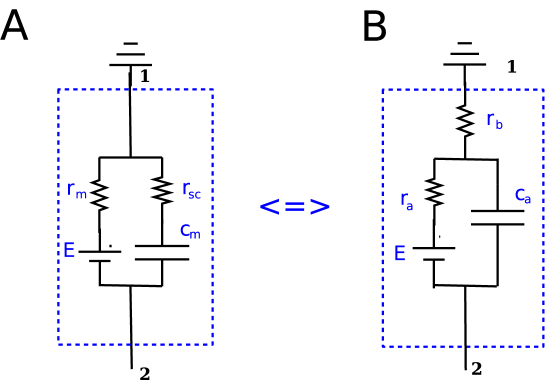
Figure 11: (Color online) Equivalence of the electrical circuits of open-circuit and non-ideal cable models. The circuits A and B are equivalent when the ratio $\frac{V_{12}(\omega)}{I(\omega)}$ of the voltage difference between points 1 and 2 and the input current between these points is invariant, and when the correspondence between the elements of these circuits are independent of frequency. Note that the values of the elements between the two circuits are related by a transformation law which is independent of frequency; this equivalence also applies to the temporal domain. In other words, according to this equivalence, the two circuits are equivalent when it is impossible to distinguish their topology from external measurements. The circuit A corresponds to the non-ideal capacitance model introduced previously BedDes2008 , while circuit B corresponds to a “standard cable model” with a short-cut (zero extracellular resistivity).

Appendix E A new interpretation of the non-ideal cable

In this appendix, we show that the non-ideal capacitance model introduced previously BedDes2008 is equivalent to an open-circuit resistive model if we assume that the circuits A and B in Fig. 11 are linked by the following transformation:

$$\left\{\begin{array}[]{cccccccc}r_{a}&=&r_{m}-\frac{r_{m}r_{sc}}{r_{m}+r_{sc}}&{}{}{}{}\hfil&r_{m}&=&r_{a}+r_{b}\\ \\ r_{b}&=&\frac{r_{m}r_{sc}}{r_{m}+r_{sc}}&{}{}{}{}\hfil&r_{sc}&=&r_{b}+\frac{r_{b}^{2}}{r_{a}}\\ \\ c_{a}&=&\frac{(r_{m}+r_{sc})}{r_{m}-\frac{r_{m}r_{sc}}{r_{m}+r_{sc}}}c_{m}&{}{}{}{}\hfil&c_{m}&=&\frac{r_{a}^{2}}{(r_{a}+r_{b})^{2}}c_{a}\end{array}\right.$$ (52)

We show that the $V_{m}$ in the non-ideal cable model corresponds to $V_{i}$ in an open-circuit (FO) type resistive model, with a reference located far-away. According to circuits A and B in Fig. 11, we have:

$$\left\{\begin{array}[]{ccc}circuit~{}A&(r_{sc}\oplus c_{m})\parallel r_{m}\\ circuit~{}B&(r_{a}\parallel c_{a})\oplus r_{b}\end{array}\right.$$ (53)

It follows that the impedances of circuits A and B are equal if we have:

$$\frac{V_{12}(\omega)}{i(\omega)}=\frac{r_{m}+i\omega r_{m}r_{sc}c_{m}}{1+i\omega c_{m}(r_{m}+r_{sc})}=\frac{r_{a}+r_{b}+i\omega c_{a}r_{a}r_{b}}{1+i\omega c_{a}r_{a}}$$ (54)

We see that the ratio $\frac{V_{12}(\omega)}{i(\omega)}$ is a homographic transform of variable $\omega$. Consequently, $\forall\omega$ we have the following relation $\frac{V_{12}(\omega)}{i(\omega)}=\frac{a_{A}+b_{A}\omega}{1+d_{A}\omega}=\frac{a_{B}+b_{B}\omega}{1+d_{B}\omega}$ when the two circuits are equivalent. The only way to guarantee that the equivalence is independent of frequency is to assume that the corresponding coefficient of the transformations are equal. We can thus set $a_{A}=a_{B}$, $b_{A}=b_{B}$ and $d_{A}=d_{B}$. This gives us 3 equations which link the 3 parameters of circuit A to those of circuit B. The solution is the transformation law (Eqs. 52). Thus, on a physical point of view, one cannot distinguish the topology of circuits A and B if we would perform external measurements. Moreover, because the functions $r_{m}=f_{m}(r_{a},r_{b}.r_{c})$, $r_{sc}=f_{sc}(r_{a},r_{b}.r_{c})$, $r_{c_{m}}=f_{c_{m}}(r_{a},r_{b}.r_{c})$ do not depend on frequency, their equivalence will be also valid for all frequencies. We can deduce that the two circuits will behave identically as a function of time .

It follows that the $V_{m}$ (between points 1 and 2) in circuit A (non-ideal capacitance) corresponds to the $V_{i}$ relative to a far-away reference in circuit B (see Table 1). Therefore, a model with non-ideal capacitance and zero extracellular resistance should produce a $V_{m}$ equivalent to the $V_{i}$ of a model with ideal capacitance and resistive extracellular medium. Thus, the frequency-scaling behavior of the $V_{m}$ obtained in a previous non-ideal cable model BedDes2008 also applies to the resistive FO model, but only if one studies the intracellular potential $V_{i}$.

Acknowledgments

Research supported by the CNRS, the ANR (Complex-V1 project) and the European Union (BrainScales FP7-269921 and Magnetrodes FP7-600730).

References

- (1)
- (2) Rall, W. (1962) Electrophysiology of a dendritic neuron model. Biophys J. 2: 145-167.
- (3) Rall, W. (1995) The theoretical foundations of dendritic function. MIT Press, Cambridge, MA.
- (4) Logothetis N.K., Kayser, C. and Oeltermann, A. (2007) In vivo measurement of cortical impedance spectrum in monkeys : implications for signal propagation. Neuron 55: 809-823.
- (5) Gabriel, S., Lau, R.W. and Gabriel, C. (1996a) The dielectric properties of biological tissues : I. Literature survey. Phys. Med. Biol.. 41 : 2231-2249.
- (6) Gabriel, S., Lau, R.W. and Gabriel, C. (1996b) The dielectric properties of biological tissues : II. Measurements in the frequency range 10 Hz to 20 GHz. Phys. Med. Biol.. 41: 2251-2269.
- (7) Bédard, C., H. Kröger, and A. Destexhe. 2006. Does the 1/f frequency scaling of brain signals reflect self-organized critical states ? Physical Review Lett. 97: 118102.
- (8) Bazhenov M, Lonjers P, Skorheim P, Bedard C and Destexhe A. (2011) Non-homogeneous extracellular resistivity affects the current-source density profiles of up-down state oscillations Phil Trans R Soc A 369: 3802-3819.
- (9) Bédard, C., Rodrigues, S., Roy, N., Contreras, D. and Destexhe, A. (2010) Evidence for frequency-dependent extracellular impedance from the transfer function between extracellular and intracellular potentials. J. Computational Neurosci. 29: 389-403.
- (10) Dehghani, N., Bédard, C., Cash, S.S., Halgren, E. and Destexhe, A. (2010) Comparative power spectral analysis of simultaneous elecroencephalographic and magnetoencephalographic recordings in humans suggests non-resistive extracellular media. J. Computational Neurosci. 29: 405-421.
- (11) Bédard, C. and Destexhe, A. (2011) A generalized theory for current-source density analysis in brain tissue. Physical Review E 84: 041909.
- (12) Bédard, C., Kröger, H. and Destexhe, A., (2006b) Model of low-pass filtering of local field potentials in brain tissue. Phys. Rev. E 73:051911.
- (13) Bédard, C. and Destexhe, A. (2009) Macroscopic models of local field potentials and the apparent 1/f noise in brain activity. Biophys. J. 96: 2589-2603.
- (14) Hines, M.L. and Carnevale, N.T (1997) The NEURON simulation environment. Neural Computation 9: 1179-1209.
- (15) Tuckwell, H.C. (1988) Introduction to Theoretical Neurobiology: Linear cable theory and dendritic structure. Cambridge University Press, Cambdridge, UK.
- (16) Bédard, C. and Destexhe, A. (2008) A modified cable formalism for modeling neuronal membranes at high frequencies. Biophys. J. 94: 1133-1143.
- (17) Johnston, D. and Wu, S.M. (1995) Foundations of cellular neurophysiology. MIT Press, Cambridge, MA.
- (18) Koch, C. (1999) Biophysics of Computation. Oxford University press, Oxford, UK.
- (19) Destexhe, A. and Bédard, C. (2012) Do neurons generate monopolar current sources ? J. Neurophysiol. 108: 953-955.
- (20) Riera, J.J., Ogawa, T., Goto, T., Sumiyoshi, A., Nonaka, H., Evans, A., Miyakawa, H. and Kawashima, R. (2012) Pitfalls in the dipolar model for the neocortical EEG sources. J. Neurophysiol 108: 956-975.
- (21) Bédard, C., Kröger, H. and Destexhe, A. (2004) Modeling extracellular field potentials and the frequency-filtering properties of extracellular space. Biophys. J. 64: 1829-1842.
- (22) Wang K, Riera JJ, Enjieu-Kadji H and Kawashima R. (2013) The role of the extracellular conductivity profiles in compartmental models for neurons: Particulars for layer 5 pyramidal cells. Neural Computation 25: 1807-1852.
- (23) Poznanski, R. (2010) Thermal noise due to surface-charge effects within the Debye layer of endogenous structures in dendrites. Physical Review E 81: 021902.
- (24) Conciauro, G. and Puglisi, M. (1981) Meaning of the negative impedance. NASA STI/Recon Technical Report 82: 14458.
- (25) Mauro, A. (1961) Anomalous impedance, a phenomenological property of time-variant resistance: An analytic review. Biophys. J. 1: 353-372.
- (26) Braitenberg, V. and A. Shutz. (1998) Cortex: Statistics and Geometry of Neuronal Connectivity. (2nd ed.), Springer-Verlag, Berlin, Germany.
- (27) Nicholson, C.. (2005) Factors governing diffusing molecular signals in brain extracellular space. J. Neural Transm. 112: 29-44.
- (28) Hiromu, M, Inoue, M., Miyakawa, H. and Aonishi, T. (2012) Low-Frequency dielectric dispersion of brain tissue due to electrically long neurites. Physical Review E 86: 061911.
- (29) Buzsaki G. (2006) Rhythms of the Brain., Oxford University Press, Oxford UK.
- (30) Walz W. (1989) Role of glial cells in the regulation of the brain ion microenvironment. Progress Neurobiol. 33: 309-333.
- (31) Kettenmann H. and Ransom BR. (1995) Neuroglia, Oxford University Press, Oxford, UK.
- (32) George, M., Lisanby, S., and Sackeim, H. (1999) Transcranial magnetic stimulation : Applications in neuropsychiatry. Arch. Gen. Psychiatry, 56 (4) :300–311.
- (33) Landau, L.D. and ifshitz, E.M. (1984) Electrodynamics of Continuous Media. Pergamon Press, Moscow, Russia.
- (34) Purcell, E.M. (1985) Electricity and Magnetism. Berkeley Physics Course Vol.2 chap. 3.