Informed and Automated k-Mer Size Selection for Genome Assembly

Abstract

Motivation: Genome assembly tools based on the de Bruijn graph framework rely on a parameter $k$, which represents a trade-off between several competing effects that are difficult to quantify. There is currently a lack of tools that would automatically estimate the best $k$ to use and/or quickly generate histograms of $k$-mer abundances that would allow the user to make an informed decision.

Results: We develop a fast and accurate sampling method that constructs approximate abundance histograms with a several orders of magnitude performance improvement over traditional methods. We then present a fast heuristic that uses the generated abundance histograms for putative $k$ values to estimate the best possible value of $k$. We test the effectiveness of our tool using diverse sequencing datasets and find that its choice of $k$ leads to some of the best assemblies.

Availability: Our tool KmerGenie is freely available at:
http://kmergenie.bx.psu.edu/

Contact: chikhi@psu.edu

1 Introduction

Genome assembly continues to be a fundamental aspect of high-throughput sequencing data analysis. In the years since the first methods were developed, there have been numerous improvements and the field is now rich with tools that provide biologists several options (Ribeiro et al., 2012; Luo et al., 2012; Bankevich et al., 2013; Chikhi and Rizk, 2012; Peng et al., 2012; Simpson and Durbin, 2011; Zerbino and Birney, 2008). Many of these tools are based on the de Bruijn graph framework, where reads are chopped up into $k$-mers (substrings of length $k$) (Pevzner et al., 2001). The de Bruijn graph is constructed with nodes being the ($k-1$)-mers and the edges being the $k$-mers present in the reads. Broadly speaking, an assembler constructs the graph, performs various graph simplification steps, and outputs non-branching paths as contigs – contiguous regions which the assembler predicts are in the genome.

Recently, there have been several meta-analyses of assemblers that have pointed to systematic shortcomings of current methods (Earl et al., 2011; Salzberg et al., 2011; Alkan et al., 2011; Bradnam et al., 2013). The Assemblathon competitions (Earl et al., 2011; Bradnam et al., 2013) demonstrated that assembling a dataset still requires significant expert intervention. One issue is many assembler’s lack of robustness with respect to the parameters and the lack of any systematic approach to choosing the parameters. In de Bruijn based assemblers, the most significant parameter is $k$, which determines the size of the $k$-mers into which reads are chopped up. Repeats longer than $k$ nucleotides can tangle the graph and break up contigs, thus, a large value of $k$ is desired. On the other hand, the longer the $k$ the higher the chances that a $k$-mer will have an error in it; therefore, making $k$ too large decreases the number of correct $k$-mers present in the data. Another effect is that when two reads overlap by less than $k$ characters, they do not share a vertex in the graph and thus create a coverage gap that breaks up a contig. Therefore, the choice of $k$ represents a trade-off between several effects.

Because some of these trade-offs have been difficult to mathematically quantify, there has not been an explicit formula for choosing $k$ taking into account all these effects. It is possible to calculate some bounds based on estimated genome size and coverage (e.g. by applying Lander-Waterman statistics), however, such estimates do not usually take into account the impact of repetitiveness of the genome, heterozygousity rate, or read error rate. In practice, $k$ is often chosen based on prior experience with similar datasets. More thorough approaches compare assemblies obtained from different $k$ values; however, they are very time consuming since a single assembly can take days for mammalian-size genomes. A more informed initial choice for $k$ can be made by building abundance histograms for putative values of $k$ and comparing them. The abundance histogram shows the distribution of $k$-mer abundances (the number of occurrences in the data) for a single $k$ value. Such histograms can provide an expert with valuable information for choosing $k$ – however, the time to construct such a histogram can take up to a day for just a single value of $k$ (Rizk et al., 2013; Marçais and Kingsford, 2011)

Our contribution in this paper is two-fold. First, we propose an accurate sampling method that constructs approximate abundance histograms with an order of magnitude speed improvement, compared to traditional tools based on $k$-mer counting. Our method allows an expert user to make an informed decision by quickly generating abundance histograms for many $k$ values and analyzing the results, either visually or statistically. Our second contribution is a fast heuristic method for selecting the best possible value of $k$, based on the generated abundance histograms for many values of $k$. The heuristic is based on the intuition that the best choice of $k$ is the one which provides the most distinct non-erroneous (genomic) $k$-mers to the assembler. Our method can be integrated into assembly pipelines so that the choice of $k$ is made automatically without user intervention.

We implement our methods in a publicly available tool called KmerGenie. We test KmerGenie’s effectiveness using three sequencing datasets from a diverse set of genomes: S. aureus, human chromosome 14, and B. impatiens. First, we find that our approximation of the histogram is very close to the exact histogram and easily separable from histograms for nearby values of $k$. Next, we judge the accuracy of KmerGenie’s choice of $k$ by assembling the data for numerous $k$ values and comparing the quality of the assemblies. We find that KmerGenie’s choice leads to the best assemblies of S. aureus and B. impatiens, as measured by the contig length (NG50), and to a good assembly of chr14 that represents a compromise between contig length and the number of errors.

2 Methods

Our method can be summarized as follows. We start by generating the abundance histograms for numerous putative values of $k$. We then fit a generative model to each histogram in order to estimate how many distinct $k$-mers in the histogram are genomic (i.e. error-free). Finally, we pick the value of $k$ which maximizes the number of genomic $k$-mers. We now describe each step in detail.

2.1 Building the abundance histograms

Consider a multiset of reads $R$ from a sequencing experiment. For a given value of $k$, each read is seen as a multiset of $k$-mers. For instance with $k=3$, the read ATAGATA is the multiset of five $3$-mers (ATA, TAG, AGA, GAT, ATA). By taking the union of all reads, a dataset of reads is also seen as a multiset of $k$-mers. Each $k$-mer is said to have an abundance, which is the number of times it appears in the multiset. A common function used to understand the role of $k$ is the abundance histogram. For a given abundance value $i$, the function tells the number of distinct $k$-mers with that abundance.

One way to calculate the abundance histogram is to first run a $k$-mer counting algorithm. A $k$-mer counting algorithm takes a set of reads and outputs every present $k$-mer along with its abundance. The abundance histogram can then be calculated in a straightforward way. $K$-mer counting is itself a well-studied problem with efficient solutions and tools, though even efficient implementations can take hours or days on large datasets (Marçais and Kingsford, 2011; Rizk et al., 2013). Such a solution would be inefficient for generating histograms for multiple values of $k$ since one would need to run the $k$-mer counter multiple times.

Instead, we propose to create an approximate histogram by sampling from the $k$-mers, an idea explored in a more general setting by Cormode et al. (2005). The pseudocode of our algorithm is shown in Algorithm 1. Intuitively, we use a parameter $\epsilon$ to dictate the proportion of distinct $k$-mers we sample. We pick a hash function $\rho_{\epsilon}:\{A,C,G,T\}^{k}\rightarrow[0..\epsilon]$ that uniformly distributes the universe of all possible $k$-mers into $\epsilon$ buckets. In our implementation, we adopted a state-less 64 bits hash function (RanHash, page 352 in (Press et al., 2007)). We then count the abundances of only those $k$-mers that hash to 0. The abundance histogram is then computed from the $k$-mer counts, scaling the number of $k$-mers with a given abundance by $\epsilon$.

0:  An integer $k>0$, a set of reads $R$, $\epsilon>0$.

0:  Approximate abundance histogram of $k$-mers in $R$

1:  Init empty hash table $T$, with default values of 0.

2:  for all $k$-mers $x$ in $R$ do

3:     if $\rho_{\epsilon}(x)=0$ then

4:        $T[x]=T[x]+1$

5:     end if

6:  end for

7:  Compute abundance histogram $h_{\epsilon}$ of $T$

8:  Let $h(i)=\epsilon\cdot h_{\epsilon}(i)$ for each $i$

9:  Output $h$

Algorithm 1 Compute approximate abundance histograms

The running time of the algorithm is $O(|R|(\ell-k))$, where $\ell$ is the read length. The expected memory usage is $O(m/\epsilon)$, where $m$ is the number of distinct $k$-mers in $R$. Though the asymptotic running time is the same as for an exact $k$-mer counting algorithm, the total overhead of adding $k$-mers to a hash table is reduced by a factor of $\epsilon$. Similarly, though the memory usage is asymptotically the same as for an exact $k$-mer counter, the decrease by a factor of $\epsilon$ can make it feasible to store the hash table in RAM.

2.2 Generative model for the abundance histogram

Given an abundance histogram, our next step is to infer the number of distinct genomic $k$-mers in it. In principle, if we knew the error rate, we could easily estimate the number of genomic $k$-mers (not necessarily distinct) as a proportion of the total number of $k$-mers. However, such a simple approach does not allow us to estimate which of the $k$-mers are genomic and hence does not allow us to estimate the number of distinct genomic $k$-mers. Moreover, the error rate is itself a parameter that is not known prior to assembly, so it must be estimated as well.

Instead, our approach is to take a generative model and fit it to the histogram. We can then infer the number of distinct genomic $k$-mers from the parameters of the model. Fitting a model to a histogram has been previously explored in the context of error-correction (Chaisson and Pevzner, 2008; Kelley et al., 2010). We adopt the model proposed by Kelley et al. (2010), which we describe here for completeness.

2.2.1 Haploid model

The $k$-mer abundance histogram is a mixture of two distributions: one representing genomic $k$-mers, and one representing erroneous $k$-mers. We use the term copy-number to denote the number of times a genomic $k$-mer is repeated in the genome. A genomic $k$-mer distribution is itself a mixture of $n$ Gaussians, each Gaussian corresponding to $k$-mers with a copy-number $1\leq i\leq n$. We fix the maximum copy-number to $n=30$. For each copy-number $i$, the mean $\mu_{i}$ and variance $\sigma_{i}^{2}$ of the Gaussian are different values (due to Illumina biases), proportional to the copy-number. Thus in our model, the mean and variance $(\mu_{1},\sigma_{1}^{2})$ (for copy-number $1$) are free parameters, and the remaining means and variances are fixed to $\mu_{i}=i\mu_{1}$ and $\sigma_{i}^{2}=i\sigma_{1}^{2}$. The weights of the mixture of Gaussians are given by a Zeta distribution, which has a single free shape parameter $s$. The erroneous $k$-mers distribution is modeled as a Pareto distribution with fixed scale of $1$ and a free shape parameter $\alpha$. The mixture between erroneous and genomic $k$-mers is weighted by a free parameter $p_{e}$, which corresponds to the probability that a $k$-mer is erroneous. Thus in total, our model has five free parameters ($\mu_{1},\sigma_{1}^{2},s,\alpha,p_{e}$).

2.2.2 Extension to the diploid model

In the diploid case, we say that a $k$-mer is homozygous if it appears in both alleles, and is heterozygous otherwise. We model the genomic $k$-mers of a diploid organism as a mixture of two haploid genomic $k$-mer distributions $D_{ht}$ and $D_{hm}$. A mixture parameter ($p_{h}$) controls the proportion of homozygous $k$-mers (drawn from $D_{hm}$) to heterozygous $k$-mers (drawn from $D_{ht}$). The parameters of the two distributions remain free, with the following exception. As homozygous $k$-mers are expected to be sequenced with twice the coverage of heterozygous $k$-mers, the mean of $D_{hm}$ is fixed to twice the mean of $D_{ht}$. As in the haploid case, we model the erroneous $k$-mers as a Pareto distribution with parameter $\alpha$ and a mixture proportion of $p_{e}$. In summary, the diploid model has eight free parameters: the variances ($\sigma_{1}^{2}$) and the Zeta shapes ($s$) for the $D_{hm}$ and $D_{ht}$ distributions; additionally, the mean ($\mu_{1}$) of $D_{ht}$, the Pareto shape ($\alpha$), the error probability ($p_{e}$), and the heterozygosity proportion ($p_{h}$).

2.3 Fitting the model to the histogram

Given the abundance histogram, we can estimate the parameters of the above model that would be the best fit for the observed histogram. Similarly to what is done in Kelley et al. (2010), we do a maximum-likelihood estimation of the parameters using the optim function in R (BFGS algorithm). Let $d$ be the number of distinct $k$-mers present in the histogram. Let $\widehat{p_{e}}$ be the estimated mixture parameter between the erroneous and genomic $k$-mers in the above model. Immediately, $\widehat{p_{e}}d$ is an estimate of the numbers of erroneous $k$-mers and $(1-\widehat{p_{e}})d$ is an estimate of the number of genomic $k$-mers present in the reads.

2.4 Finding the optimal $k$

Our key insight is that the best value of $k$ for assembly is the one which provides the most distinct genomic $k$-mers. To see this, consider the number of distinct $k$-mers in the reference genome. Observe that, as $k$ increases, this number also increases and approaches the length of the genome, as a consequence of repeat instances becoming fully spanned by $k$-mers. Thus, a high number of distinct genomic $k$-mers allows the assembler to resolve more repetitions. In the ideal scenario of perfect coverage and error-free reads, the best value of $k$ for assembly would be the read length. However, the read coverage is typically imperfect and reads are error-prone, requiring a more nuanced approach.

First, consider obvious high and low thresholds: for $k$ close to the read length, it is unlikely that all the $k$-mers in the reference are present in the reads due to imperfect coverage. On the other hand, note that any genome will contain all $k$-mers for a small enough $k$ (e.g. the human genome contains all possible $4$-mers). This is due to the fact that a significant chunk of a genome behaves like a random string.

Next, we examine the values of $k$ between these two thresholds. Essentially, two effects are competing. The shorter a $k$-mer is, the more likely it is (i) to appear in the reads, but also (ii) to be repeated in the reference. For a typical sequencing depth and values of $k$ near the read length, it is likely that only a small fraction of the $k$-mers from the reference genome appears in the reads (effect (i)). However, unless the sequencing depth is insufficient for assembly, there exists of a largest value $k_{0}$ at which nearly all the $k$-mers in the reference genome are present in the reads for $k\leq k_{0}$. Thus, decreasing $k$ below $k_{0}$ only contributes to making more $k$-mers repeated (effect (ii)).

From these observations, we conclude that the number of distinct genomic $k$-mers in the reads is likely to reach a maximum value. At this value, all the $k$-mers in the reference genome are likely to appear in the reads, thus the assembly at this $k$-mer length nearly covers all the genome. Also, the assembly is likely to be of high contiguity as a large number of distinct $k$-mers imply that more repetitions are fully spanned by $k$-mers.

3 Results

3.1 Datasets and assemblers

We benchmarked KmerGenie using data from the Genome Assembly Gold-standard Evaluation (GAGE), which was previously used to evaluate and compare different assemblers (Salzberg et al., 2011). We used three datasets from three genomes of different sizes: S. aureus (2.8 Mbp), human chromosome 14 (88 Mbp) and B. impatiens (250 Mbp). The datasets contain 5mil/62mil/497mil Illumina reads of length 101bp/101bp/124bp (respectively). The coverages are 167x/70x/247x.

For each dataset, the GAGE study published the assembler that produced the best results, along with its most effective formula (including commands and parameters). To assess how our predicted $k$ values relate to the quality of assemblies, we choose, for each dataset, the de Bruijn assembler and formula that produced the best results in the GAGE study. For S. aureus and chr14, this was Velvet 1.2.08 (Zerbino and Birney, 2008) with the parameters given on the GAGE website. For B. impatiens, we used SOAPdenovo2 (Luo et al., 2012) using the GAGE recipe and no additional parameters. All experiments were run on a 32-core machine (Xeon E7-8837 @ 2.67 GHz) with 512GB RAM.

3.2 Performance of KmerGenie’s choice of $k$

We ran KmerGenie on all three datasets with putative $k$ values of $21,31,41,51,61,71,81$ and a sampling frequency of $\epsilon=1000$. The optimal values of $k$ were predicted to be 31 for S. aureus, 71 for chr14, and 51 for B. impatiens. We then assembled each dataset using both the optimal and other reasonable values of $k$. The results of each assembly are shown in Table 3.2. The decision of what constitutes a “best” assembly is complicated due to the inherent trade-offs (Salzberg et al., 2011; Earl et al., 2011; Bradnam et al., 2013). We therefore evaluated each assembly using three common quality measures: the contig NG50 length, the assembly size, and the number of assembly errors. Contig NG50 is defined as the length at which half of the predicted genome size is contained in contigs longer than this length. Contigs were obtained by splitting reported scaffolds at each undetermined nucleotide. The size was measured as the sum total length of contigs larger than $500$ bp. The Error column reflects the number of mis-joins called by the QUAST software (Gurevich et al., 2013). Note that for B. impatiens there is no reference available and hence it is not possible to measure the number of errors. QUAST reports an assembly error as a position in the assembled contigs where one of the following mis-assembly events occur: (i) the left flanking sequence aligns over 1 kbp away from the right flanking sequence on the reference, or (ii) they overlap by $>1$ kb, or (iii) the flanking sequences align on opposite strands or different chromosomes.

Assembly	Contig NG50 (Kbp)	Size (Mbp)	Errors
S. aureus (Velvet)
$k=21$	0.5	7.65	0
$k=31$	19.4	2.83	10
$k=41$	11.7	2.81	6
$k=51$	4.6	2.80	9
chr14 (Velvet)
$k=41$	2.4	74.56	764
$k=51$	4.0	79.92	843
$k=61$	5.4	82.10	431
$k=71$	4.7	81.89	251
$k=81$	1.8	74.18	153
B. impatiens (SOAPdenovo2)
$k=41$	5.4	224.05
$k=51$	10.4	229.71
$k=61$	9.5	230.36
$k=71$	5.9	226.11
$k=81$	2.5	207.11

Table 1: Quality of assemblies for different values of $k$. The value of $k$ predicted by KmerGenie is underlined.

For S. aureus, the assembly with the chosen $k$ had the best NG50 and size, but had more errors than other assemblies. For chr14, the assembly with the chosen $k$ did not have the best NG50 or size (though it was close), but did have significantly less errors. For B. impatiens, the chosen $k$ gave an assembly with the best NG50 and second best size (the number of errors is unknown since there is no reference). Overall, KmerGenie’s choice of $k$ led to the best assemblies of S. aureus and B. impatiens, as measured by the NG50 and assembly size, and to a good assembly of chr14 that represents a compromise between NG50/assembly size and the number of errors.

KmerGenie is multi-threaded, it uses one thread per $k$ value. For a single thread, the running time and memory usage of KmerGenie is shown in Table 2. We also compared the speed of our approximate histogram generation to what could be achieved by the exact $k$-mer counting method DSK (Rizk et al., 2013). KmerGenie ran 6-10 times faster than DSK, confirming that our sampling approach leads to significant speed-ups. For the largest dataset (B. impatiens), the total wall-clock time of KmerGenie with $k$-mer set $\{21,31,41,51,61,71,81\}$ using 7 threads is 3 hours. Note that assembling B. impatiens using SOAPdenovo2 requires approximately 30 CPU hours for a single value of $k$ (10 wall-clock hours, 8 threads).

Organism	CPU time		Memory usage of
	DSK	KmerGenie	KmerGenie (GB)
S. aureus	2min	11sec	0.1
chr14	48min	7min	0.1
B. impatiens	7.5hour	1.2hour	0.4

Table 2: Resource utilization of KmerGenie compared to a $k$-mer counting based approach (DSK).We executed KmerGenie and DSK for a single value of $k$ (81) using one thread. KmerGenie was executed with a sampling frequency of $\epsilon=1000$. DSK used $5$ GB of memory.

3.3 Comparison with VelvetOptimizer and VelvetAdvisor

We are aware of only two other methods that have been proposed to optimize $k$. VelvetOptimizer (abbreviated VO) is an unpublished tool that attempts to optimize $k$ by performing a Velvet assembly for each odd $k$ value between 19 and 79 and picking the one that yields the highest scaffold N50 (Seemann, http://dna.med.monash.edu.au/~torsten/velvet_advisor). It then determines coverage cut-off parameters that yield the longest assembly in contigs longer than 1 kbp. Since this requires doing 30 assemblies, using VO on the chr14 data would require close to half a CPU-year. We therefore were not able to evaluate VO on chr14 or the even larger B. impatiens.

We did execute VO on the S. aureus dataset, using the default optimization parameters. Each Velvet assembly requires around 40 minutes of CPU time, resulting in 20 hours computation (though this can be parallelized). VO selected the assembly with $k=41$, with expected coverage value of $12$, and cut-off value of $6.47$. Compared to the assembly based on KmerGenie’s choice of $k=31$ (shown in Table 3.2), VO’s assembly has slightly higher size (2.85kbp vs 2.83kbp), significantly lower contig NG50 (11.6kbp vs 19.4kbp), and significantly more errors (23 vs 10). The VO assembly has a higher scaffold N50 (734 kbp versus 257 kbp), but this high N50 value may be misleading: QUAST reports a NGA50 value (corrected scaffold NG50) of 11.6 kbp for the VO assembly, and 110.2 kbp for KmerGenie assembly. We conclude that KmerGenie’s choice of $k$ leads to a better assembly than VO’s in this case. We note, however, that we believe the main advantage of KmerGenie over VO’s approach is that it is orders of magnitude faster (2mins vs 20 hours) and is applicable even when VO is not feasible (e.g. chr14 and B. impatiens).

Another method is the unpublished tool Velvet Advisor (Gladman and Seemann, http://bioinformatics.net.au/software.velvetoptimiser.shtml). It uses a formula to recommend a value of $k$, given the number of reads, the read length and the estimated genome length. Velvet Advisor recommends $k=81$ for the S. aureus dataset, $k=51$ for the chr14 dataset and $k=85$ for the B. impatiens dataset. The $k$ value for the chr14 dataset leads to a good assembly, but, for S. aureus and B. impatiens, the assemblies using these values are very poor.

3.4 Effect of sampling and the fit of the statistical model

Since the main purpose of the histograms is to contrast the differences between different $k$ values, we measure the accuracy of our approximate histogram by comparing it at a fixed $k$ value (51) to the exact distribution of $k=51$ and the exact distributions of nearby $k$ (41 and 61). The results for our three datasets are shown in Figure 1. We observe that the sampled histogram closely follows the exact one and easily discriminates between other $k$ values when such a discrimination is possible from the exact counts.

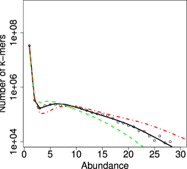
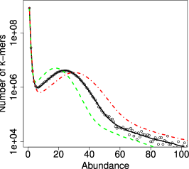
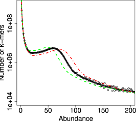
Figure 1: The accuracy of the sampling method. The panels reflect the three datasets: S. aureus (a), chr14 (b), and B. impatiens (c). Each plot show the exact histogram curves for $k=51$ (solid black curve), $k=41$ (dash-dot red curve), and $k=61$ (dashed green curve). The approximate (sampled) histogram is shown using black dots. Note that $y$ is shown on a log-scale, exaggerating the differences at lower y values.

We illustrate the effect of $k$ on the abundance histogram for chr14 in Figure 2. In this case, the histogram is dominated by a mixture of a distribution for erroneous $k$-mers and one for genomic $k$-mers. As $k$ increases, the genomic distribution shifts left and becomes more narrow, resulting in a larger overlap with the erroneous distribution.

Figure 2: The abundance histograms for chr14 with $k$ values of 21, 41, and 81 (on a y log scale). Each plot also shows a curve corresponding to the optimized statistical model (haploid).

Figure 2 also shows the fit of our model to the histogram. Even though the human genome is diploid, its heterozygosity rate is small enough that we model the $k$-mer abundance histogram using the haploid statistical model. The high copycounts appear to be inaccurately fitted, but note that the log-scale amplifies the difference in low abundances. For B. impatiens, on the other hand, the haploid model does not lead to a good fit, likely due to a possibly higher polymorphism rate. Figure 3 shows the difference in fit between using a haploid and diploid model for B. impatiens.

Figure 3: The abundance histogram and optimized model for B. impatiens, $k=41$, using a haploid (left) and a diploid model (right), on a y log scale. In both graphs, the black histogram curves are the actual $k$-mer histogram, and the red (solid) curve is the maximum likelihood fit using our model. In the diploid model graph, the green (dot-dashed) curve models the heterozygous $k$-mers, and the blue (dashed) curve models the homozygous $k$-mers. Other components of the mixture are not shown.

3.5 Relation of the number of distinct genomic $k$-mers to assembly quality

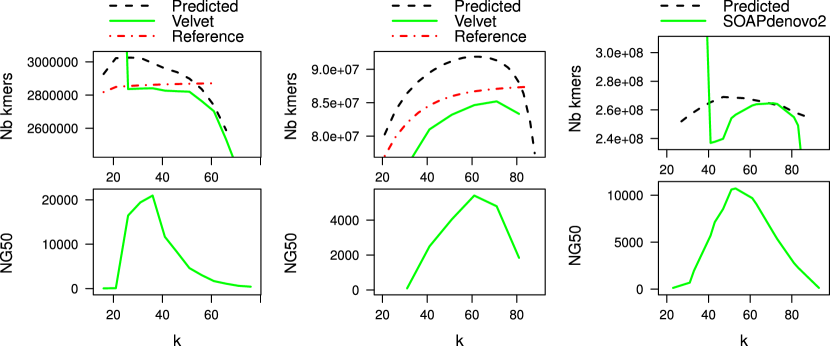
Figure 4: Relation of the number of distinct genomic $k$-mers to assembly quality. We show the results for the three datasets: S. aureus (left), chr14 (middle), B. impatiens (right). We plot the number of distinct genomic $k$-mers predicted from the histogram from our model, the number present in the reference, and the number present in the assembly. We also show the NG50 of the assembly.

An important component of our method is the prediction of the number of distinct genomic $k$-mers from the abundance histogram. Our underlying assumption is that providing the assembler with more distinct genomic $k$-mers leads to more of these $k$-mers being used in contigs and to longer contigs. To measure this effect, we plot (as a function of $k$) the number of distinct genomic $k$-mers predicted from the histogram, the number of distinct $k$-mers used in the assembly, the NG50 of the assembly, and the number of distinct $k$-mers in the reference (Figure 4).

For S. aureus and chr14, the number of distinct genomic $k$-mers in the assembly approximatively mirrors the number of ones predicted in the input, with the exception of extreme $k$ values. For B. impatiens, the variations of the predicted number of $k$-mers do not match the variations of the number of distinct $k$-mers present in the assemblies. We postulate that this discrepancy may be due to heterozygosity, and note that the agreement between NG50 and our prediction is sufficient for our purpose.

For all three organisms, the NG50 rises and falls in accordance with the number of predicted distinct genomic $k$-mers. We also observe that KmerGenie overestimates the number of distinct genomic $k$-mers when compared to the reference $k$-mers. A part of this is likely due to heterozygosity, which is not captured in the haploid reference. However, it may also partially indicate room for improvement in our statistical model and/or optimization.

For the lowest values of $k$ in the S. aureus and B. impatiens datasets, the assemblers produce a much larger assembly than expected. We conjecture that this is due to a mis-estimation in the assemblers of what constitutes an erroneous $k$-mer (since with low $k$-mer sizes, erroneous $k$-mer have higher abundance than with high $k$-mer sizes). We verified this conjecture in the S. aureus dataset, by manually assembling S. aureus with Velvet using $k=21$ and a larger coverage cut-off value forced to 7 (experimentally found). The new Velvet assembly size is $2.8$ Mbp, which is much closer to the reference size than the $7.65$ Mbp assembly with automatic coverage cut-off. Thus, this indicates that larger assemblies are artifacts made by assemblers rather than an actual increase of genomic $k$-mers.

4 Discussion

While we have presented a method that attempts to find the best value of $k$ for assembly, we would like to note several limitations inherent in this approach. First of all, KmerGenie may in some instances report that a best value of $k$ cannot be found because it is not able to fit the generative model to the abundance histograms. This could simply be due to a limitation of our model or the optimization algorithm, but it could also be due to a difficulty inherent in the data. For example, data from single cell experiments have uneven coverage (Chitsaz et al., 2011), violating a basic assumption of our model. Similarly, data from metagenomic or RNA-seq experiments do not come from a single genome and their histograms have different properties. In these cases, it has been observed that there is often no single best $k$ and and that combining the assemblies from different $k$ can be beneficial. Though KmerGenie does not suggest a $k$ in these cases, it provides the abundance histograms that can be useful in determining the best assembly approach.

We have demonstrated our approach to be useful for de Bruijn based assemblers. Other assemblers, such as SGA (Simpson and Durbin, 2011), follow the alternate string overlap graph approach, in which reads are not chopped up into $k$-mers. These assemblers do not have the $k$ parameter but do have an alternate parameter for the minimum length of a non-spurious overlap. Though a formal relation between these parameters has not been established, they play a similar role in affecting the assembly results. We therefore consider it an interesting direction for future research to extend our approach to select the best overlap parameter for string overlap graph assemblers.

Finally, we wish to emphasize that our benchmark did not attempt to produce the best possible assembly for each organism. Rather, we are restricting ourselves to what a “typical” user might do with the data: run a single assembly software on un-corrected data, and possibly try several $k$-mer values. In order to get the best possible assembly, one would have to explore the Cartesian product of several assemblers, several read error-correction methods, and several $k$-mer values, which is often a prohibitively long task. Notably, because we did not select the best error-correction method for each assembler/organism, the assemblies reported in Table 3.2 have lower contig N50 (and also scaffold N50, data not shown) than those reported in the GAGE benchmark.

There are improvements that we have left for future work. The first direction is to determine how our method could be applied to non-uniform coverage. While a single best $k$ value for metagenome and transcriptome assembly is unlikely to exist, perhaps useful information could be extracted from the histograms constructed on such datasets. The second direction is to explore ways of improving the accuracy of our statistical model, potentially leading to more accurate estimates of the number of distinct genomic $k$-mers.

Acknowledgements

We would like to thank Qunhua Li and Francesca Chiaromonte for useful discussions.

References

- Alkan et al. [2011] Can Alkan, Saba Sajjadian, and Evan E Eichler. Limitations of next-generation genome sequence assembly. Nature Methods, 8:61–65, 2011.
- Bankevich et al. [2013] Anton Bankevich, Sergey Nurk, Dmitry Antipov, Alexey A Gurevich, Mikhail Dvorkin, Alexander S Kulikov, Valery M Lesin, Sergey I Nikolenko, Son Pham, Andrey D Prjibelski, Alexey V Pyshkin, Alexander V Sirotkin, Nikolay Vyahhi, Glenn Tesler, Max A Alekseyev, and Pavel A Pevzner. SPAdes: A new genome assembly algorithm and its applications to single-cell sequencing. Journal of Computational Biology, 19(5):455–477, 2013.
- Bradnam et al. [2013] Keith R Bradnam et al. Assemblathon 2: evaluating de novo methods of genome assembly in three vertebrate species. arXiv preprint arXiv:1301.5406, 2013.
- Chaisson and Pevzner [2008] Mark J Chaisson and Pavel A Pevzner. Short read fragment assembly of bacterial genomes. Genome research, 18(2):324–330, 2008.
- Chikhi and Rizk [2012] Rayan Chikhi and Guillaume Rizk. Space-efficient and exact de Bruijn graph representation based on a bloom filter. In WABI, pages 236–248, 2012.
- Chitsaz et al. [2011] Hamidreza Chitsaz et al. Efficient de novo assembly of single-cell bacterial genomes from short-read data sets. Nature Biotechnology, 29:915––921, 2011.
- Cormode et al. [2005] Graham Cormode, S Muthukrishnan, and Irina Rozenbaum. Summarizing and mining inverse distributions on data streams via dynamic inverse sampling. In Proceedings of the 31st international conference on Very large data bases, pages 25–36. VLDB Endowment, 2005.
- Earl et al. [2011] D. A Earl, K. Bradnam, J. S John, A. Darling, D. Lin, J. Faas, H. O.K Yu, B. Vince, D. R Zerbino, and M. Diekhans. Assemblathon 1: A competitive assessment of de novo short read assembly methods. Genome Research, 2011.
- Gurevich et al. [2013] Alexey Gurevich, Vladislav Saveliev, Nikolay Vyahhi, and Glenn Tesler. QUAST: quality assessment tool for genome assemblies. Bioinformatics, 2013.
- Kelley et al. [2010] David R Kelley, Michael C Schatz, and Steven L Salzberg. Quake: quality-aware detection and correction of sequencing errors. Genome Biol, 11(11):R116, 2010.
- Luo et al. [2012] Ruibang Luo, Binghang Liu, Yinlong Xie, Zhenyu Li, Weihua Huang, Jianying Yuan, Guangzhu He, Yanxiang Chen, Qi Pan, Yunjie Liu, et al. SOAPdenovo2: an empirically improved memory-efficient short-read de novo assembler. GigaScience, 1(1):1–6, 2012.
- Marçais and Kingsford [2011] Guillaume Marçais and Carl Kingsford. A fast, lock-free approach for efficient parallel counting of occurrences of k-mers. Bioinformatics, 27(6):764–770, 2011.
- Peng et al. [2012] Yu Peng, Henry C. M. Leung, S. M. Yiu, and Francis Y. L. Chin. IDBA-UD: a de novo assembler for single-cell and metagenomic sequencing data with highly uneven depth. Bioinformatics, 28(11):1420–1428, 2012.
- Pevzner et al. [2001] Pavel A. Pevzner, Haixu Tang, and Michael S. Waterman. An Eulerian path approach to DNA fragment assembly. Proceedings of the National Academy of Sciences, 98(17):9748–9753, 2001.
- Press et al. [2007] William H Press, Saul A Teukolsky, William T Vetterling, and Brian P Flannery. Numerical recipes 3rd edition: The art of scientific computing. Cambridge University Press, 2007.
- Ribeiro et al. [2012] Filipe Ribeiro, Dariusz Przybylski, Shuangye Yin, Ted Sharpe, Sante Gnerre, Amr Abouelleil, Aaron M Berlin, Anna Montmayeur, Terrance P Shea, Bruce J Walker, Sarah K Young, Carsten Russ, Iain MacCallum, Chad Nusbaum, and David B Jaffe. Finished bacterial genomes from shotgun sequence data. Genome Research, 2012.
- Rizk et al. [2013] Guillaume Rizk, Dominique Lavenier, and Rayan Chikhi. DSK: k-mer counting with very low memory usage. Bioinformatics, 29(5):652–653, 2013.
- Salzberg et al. [2011] S. L Salzberg, A. M Phillippy, A. Zimin, D. Puiu, T. Magoc, S. Koren, T. J Treangen, M. C Schatz, A. L Delcher, and M. Roberts. GAGE: a critical evaluation of genome assemblies and assembly algorithms. Genome Research, 2011.
- Simpson and Durbin [2011] Jared T Simpson and Richard Durbin. Efficient de novo assembly of large genomes using compressed data structures. Genome Research, 2011.
- Zerbino and Birney [2008] Daniel R Zerbino and Ewan Birney. Velvet: algorithms for de novo short read assembly using de Bruijn graphs. Genome research, 18(5):821–829, 2008.