An Interferometric Analysis Method for Radio Impulses from Ultra-high Energy Particle Showers
Abstract
We present an interferometric technique for the reconstruction of ultra-wide band impulsive signals from point sources. This highly sensitive method was developed for the search for ultra-high energy neutrinos with the ANITA experiment but is fully generalizable to any antenna array detecting radio impulsive events. Applications of the interferometric method include event reconstruction, thermal noise and anthropogenic background rejection, and solar imaging for calibrations. We illustrate this technique with applications from the analysis of the ANITA-I and ANITA-II data in the 200-1200 MHz band.
keywords:
radio, interferometry, neutrinos, cosmic-rays1 Introduction
In the last decades there has been an increased interest in using radio frequency (RF) instrumentation for the detection of ultra-high energy (UHE) eV neutrinos and cosmic rays. Russian-Armenian physicist Gyurgen Askaryan [1] predicted that high energy particle showers produced in dense dielectric media would result in impulsive coherent Cherenkov radiation at radio frequencies. The emission was experimentally confirmed for the first time in 2001 using showers induced by high energy photons in silica sand [2]. The results are consistent with modern particle shower and radio emission simulations [3] and this effect has since been observed in salt [4] and ice [5]. Several experiments exploit this technique in the search for UHE neutrinos using antennas buried in ice [6, 7], radio telescopes pointed at the Moon [8, 9], or balloon-borne antenna arrays orbiting the Antarctic continent [10].
Cosmic ray extensive air showers (EAS) produce a radio impulse due to the transverse current produced by the separation of electrons and positrons resulting from interaction with the Earth’s magnetic field [11, 12]. This geo-synchrotron emission was first observed in a ground array in the 1960’s [13]. Since then, there have been many observations [14]-[25]. Recently, the Antarctic Impulsive Transient Antenna (ANITA), a balloon-borne antenna array that synoptically scans the Antarctic continent in the 200-1200 MHz range, observed geo-synchrotron emission in the ultra-high energy range for the first time [26].
The growth of this field demands improved analysis techniques. In particular, it is expected that the first neutrino observations will be from signals that are close to the detector threshold set by thermal noise. This requires analysis techniques that are highly sensitive and can efficiently discriminate between a weak impulse and a thermal fluctuation.
Interferometric methods have been widely and successfully used in radio astronomy. Radio telescopes are able to map weak sources in the sky using the correlations between signals in an antenna array. Distant sources are imaged via the relation between phase delay and source direction [27]. Additional point-spread deconvolution methods are applied to reveal high resolution brightness maps of the radio source. The most precise astrometric measurements (200 -arcsec resolution) are obtained from the correlations of a single pair of antennas with 8,000 km separation [28].
The signals produced by UHE particle showers are rather different from those detected by radio interferometric telescopes. UHE particle shower emissions are impulsive transient events (on microsecond to nanosecond time scales) while radio astronomical sources are better described as brightness distributions that can be imaged with long exposures. Despite the differences in the nature of these signals, the fundamental ideas of radio interferometry can be applied to the detection and analysis of UHE particle shower impulsive transient events.
An interferometric approach for impulsive signals was developed for ANITA and successfully applied to the data analysis of both flights [26, 29]. The ANITA antenna array is designed to observe impulsive radio emission in the frequency range 200-1200 MHz from UHE neutrinos interacting in the Antarctic ice. Each antenna is a dual-polarized quad-ridged horn with a gain of 10 dBi and a half-power beam-width of . The ANITA array is cylindrically symmetric with neighboring antennas that have a center-to-center distance of 1 meter. Typical antenna separations used in the direction reconstruction are 5 meters for ANITA-I [10] and 7 meters for ANITA-II [29] producing a pointing error below .
In the interferometric imaging procedure developed for ANITA, each pair of antennas produces a fringe across the sky at an angle corresponding to the baseline direction111A baseline is the vector defined by an antenna pair.. The fringes are then summed together resulting in an image that peaks at the source location. Such an image is named a “dirty map” in radio astronomical usage, and reduction of sidelobes is possible with further image processing. However, we have found that for this type of “pulse-phase interferometry” [10], these maps are adequate since the sources of interest to ANITA are unresolved. It is also worth mentioning that ANITA does not apply this mapping to identify and characterize source structure but rather for the identification of coherent point source impulses. We also rely on the point-like characteristics of our data and delay closure to calibrate antenna positions and cable delays [10].
Although there have been other impulse beam-forming results in the past, particularly the one developed for imaging the radio flashes from ultra-high energy cosmic rays (UHECRs) for the LOPES antenna array [30], there are some important differences with the variant developed in this paper. ANITA is a self-triggering array and does not have muon counter data for identifying UHECR signals. The interferometric techniques developed for ANITA are applied as a stand-alone technique for identifying plane wave impulses in the data and for refining the precision of the directional reconstruction while providing improved rejection of thermal noise and anthropogenic backgrounds.
This paper presents an interferometric method applicable to broadband, impulsive radio signals for antenna arrays with large fields of view and digital waveform recording capabilities. The technique is illustrated via its application to the ANITA analysis. In Section 2 the mathematical foundations of the interferometric image production applied to radio impulses are covered. Section 3 describes the application of interferometric images to point source impulse reconstruction along with rejection of thermal noise and anthropogenic backgrounds. Section 4 presents an application of the interferometric method to identify and characterize sources that are below detection threshold but continually present. We demonstrate the technique with observations of the Sun and images of RF activity on the Antarctic continent. In Section 5 we conclude this paper and mention some future applications of the interferometric technique developed here.
2 Interferometric Equation
In this section we formulate the interferometric approach used for radio impulses. At its core, interferometry is based on combining multiple measurements of the same signal. We discuss the relation between a recorded voltage and an electric field followed by the relation between the Adding Interferometer and a Cross-Correlation Interferometer in the context of radio impulse detection. We motivate the approach used for the analysis of ANITA data. It is worth noting, that unlike typical interferometric arrays, the ANITA antennas are not all pointing in the same direction as their boresight direction varies with payload azimuth to provide a full 360∘ field of view coverage [10]. In general, this would require that the system impulse response be deconvolved prior to beam-forming. However, we argue that for the ANITA horn antennas this is not necessary. The tools described below can just as well be applied with prior deconvolution of the antenna response but not requiring this step makes their application practical.
2.1 Relation between the electric field and receiver voltage
An incident electric field couples to the antenna inducing surface currents that produce voltage differences in a transmission line that can be stored in a recording apparatus. Since ANITA is primarily concerned with ultra-wide band impulses it is natural to approach the problem in the time-domain. A detailed time-domain treatment of the relation between an electric field and the voltage recorded in an experiment can be found in [31] and references therein. The relation is captured via
| (1) |
where is the load impedance, is the impedance of free space, and is the direction of incidence of the radiation. The effective height vector is the time-domain representation of the antenna receiver system complex impedance, and is equivalent to the antenna receiver system response to a delta-like pulse [31]. The operator is a vector convolution defined by . We have made explicitly a function of since, in general, the effective height depends on the angle of incidence of the electric field with respect to the antenna. The measured voltage recorded with a digitizer is, strictly speaking, a function of time only; the added dependence of on captures the fact that the frequency contents and group delay of the effective height depends on the direction of incidence of the radiation relative to the antenna.
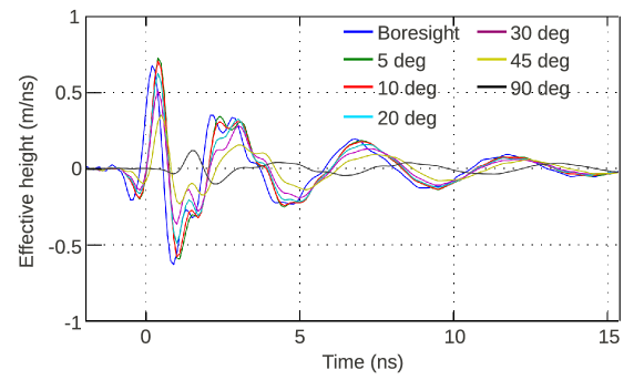
Figure 1 shows the time-domain effective height for various incidence angles for an ANITA quad-ridged horn antenna. It is important to note that Figure 1 shows the effective height of the antenna alone and does not include the system response of the full signal chain with cables, filters, and amplifiers. The low frequency dispersion (corresponding to the frequency range 200-300 MHz) extends for about 10 ns on the tail end of the waveform while the high frequency (300-1200 MHz) portion the signal is contained within the first few nanoseconds. Note, however, that the effective height dispersion is nearly identical for signals up to 45∘ away from boresight. This means that, for the purposes of correlating signals, the antenna response does not need to be corrected within this angular range. The only significant difference in the effective height function, for the various observation angles within 45∘ away from boresight, is the attenuation of high frequencies. This feature is equivalent to the antenna beam pattern being narrower for high frequencies and wider for lower frequencies.
2.2 Mapping the incident signal direction using receiver voltages
The similarity between waveforms due to the same signal in the antenna array is at the foundation of interferometry. Radio telescope interferometers typically use the pairwise cross-correlation between signals recorded at each antenna where the waveforms are delayed according to a given direction and multiplied together. Another variant is to use the Adding Interferometer where the waveforms of each antenna are delayed, summed together, and the square of the sum is integrated. Summing the waveforms, delayed according to the direction of incidence, averages down the noise while coherently adding the signal, providing an improved signal to noise ratio222We define the signal to noise ratio of an impulse by the half maximum peak to peak voltage difference divided by the root mean square of the noise. (SNR). This summed waveform has the clear advantage of exposing a weak signal measured by a number of antennas. In this section we derive various interferometric quantities from this starting point. Although the quantities associated with the Adding and Cross-Correlation Interferometers are well known in the literature [27], we re-derive them here in the context of radio impulses to motivate the analysis techniques used in the next section.
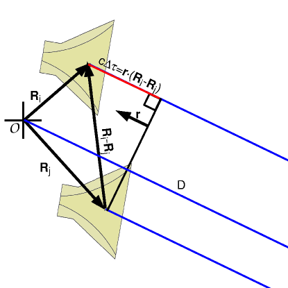
Let us describe the data of an array of antennas by a set of voltages for each antenna . For a plane wave incident from direction the delay at each antenna is given by
| (2) |
where is the distance between the source and the antenna array, is the antenna position, as shown in Figure 2, and is the speed of light. The phase aligned voltage waveforms are to be summed together to give the coherently summed waveform
| (3) |
If the voltage waveforms are only due to uncorrelated noise between the antennas, with the same root-mean-square (RMS) voltage , then has an RMS increased by a factor of the , regardless of the delays between them. If the voltage waveforms all contain the same plane wave signal impulse, then will be equal to times when the delays correspond to the direction of incidence of the signal. Thus, on average, a set of waveforms with the same noise RMS and the same signal will result in with an amplitude enhanced by a factor over each individual .
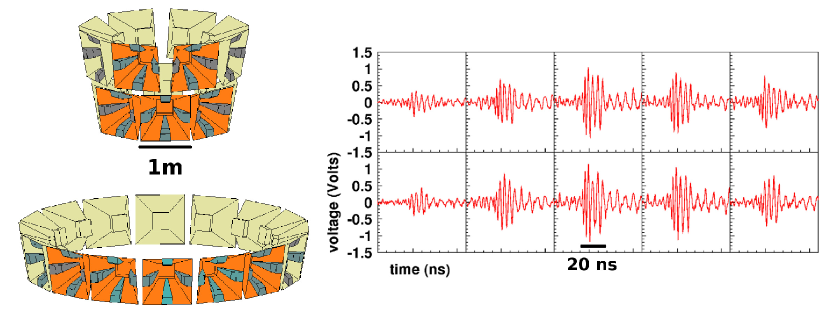
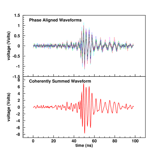
Figure 3 shows a model of the ANITA horn antenna array with ten signals highlighted. The event shown is sent from a ground-based calibration pulser used for testing pointing reconstruction techniques. The top panel of Figure 4 shows the phase (or delay) aligned waveforms using the known direction of incidence, which are summed to give the coherently summed waveform shown on the bottom panel of Figure 4.
One could formulate an analysis based on finding the peak of as a function of , but in reality signals are not perfect delta functions and display some dispersion due to the antenna, the signal chain, or the neutrino induced shower itself [32]. For this reason, one can obtain a higher SNR measurement using the power of integrated over a time window relevant to the impulses of interest.
The time averaged power of the summed receiver voltages is
| (4) |
where is the total time of the integration and is the impedance of the system. The quantity is also known as the Adding Interferometer.
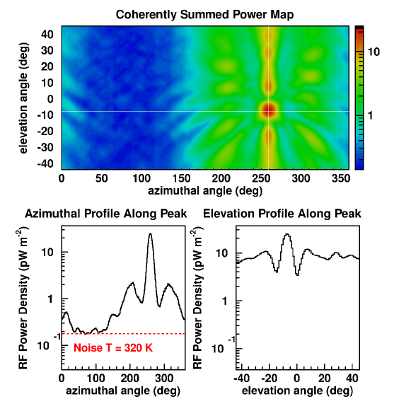
Figure 5 shows the power map for a flight calibration impulse from the ANITA-I flight. A set of ten antennas centered around each -sector333ANITA is divided into 16 -sectors, each consisting of a pair of antennas on top and on bottom (see left side of Figure 3). ANITA-II has a third tier of antennas on every other -sector, shown in Figure 3, is used for the summed waveform as a function of direction. The power map shows the most likely direction of incidence as a large peak with sidelobes representative of the system’s point spread function determined by the geometrical arrangement of the antennas and the interference pattern of the waveforms. At angles away from the direction of incidence of the impulse, the image shows the typical random pattern produced by thermal noise. Note that this approach has ignored the differences in effective height between antennas pointing in different directions. This is because the ANITA horn antenna response does not significantly vary in phase at different incident angles444Finite Difference Time Domain simulations of the impulse response of the ANITA horns found 45 ps delays between signals incident on boresight and at 22.5∘ away. At 2.6 Gsa/s the digitization time bin width is 384 ps.. It also allows for faster computation which is advantageous when dealing with large data sets.
In the context of mapping brightness distributions, the Adding Interferometer has the potentially undesirable feature of including the noise from each individual waveform. It also has undesirable effects when the gain and noise figures in each channel are not matched. Although can be a useful quantity for the analysis of radio impulses, given that the proper calibrations have been made, we can also remove some of its potentially inconvenient qualities with some mathematical manipulations.
The time averaged power of the summed receiver voltages in Equation 4 can be expanded to give
| (5) |
where and are the delays with respect to the origin of a given coordinate system in Equation 2. The terms on the right hand side of the equation are proportional to the cross-correlations between antenna voltages defined as
| (6) |
where . Note that the term , in Equation 2, denoting the distance from the source to the array vanishes. Substituting Equation 6 into Equation 5, reduces to
| (7) |
where
| (8) |
is the average power of each individual waveform, which does not depend on given that . The cross-correlation (also known as cross-power) term contains the directional information of the electric fields incident on the antenna array.
If we only keep the terms that depend on the direction of incidence in Equation 7, we obtain cross-correlation map
| (9) |
where the restriction counts each baseline once. However, the quantity retains undesirable features if the gains and noise figures of each channel are not matched.
Another approach is to normalize the cross-correlation by the power of the waveform according to
| (10) |
which is known as the the cross-correlation coefficient or coherence function [33]. This value is bounded between a maximum value of +1 and a minimum value of -1 and quantifies the similarity between waveforms and . If the waveforms are identical the cross-correlation coefficient is +1. If they are identical with a 180∘ phase difference then it is equal to -1. The more dissimilar the waveforms, the closer the cross-correlation coefficient is to zero.
The power sum can be written in terms of the cross-correlation coefficients as
| (11) |
In this sense the cross-correlation coefficients naturally quantify the interference terms in the coherent power sum. The terms are not sensitive to the overall amplitude scale of the waveforms, which can vary due to thermal fluctuations. The terms contain all the directional information provided by of the Adding Interferometer or of the Cross-Correlation Interferometer.
For the ANITA analysis it was found that the cross-correlation coefficient was the best means of reconstructing the direction of a signal [10, 34, 26, 29]. The attractive features are that it normalizes out overall amplitude fluctuations along with mismatched gains and noise figures. In addition, its statistical behavior is not strongly affected by the moderate use of notch filters.
Another way to produce interferometric images is to project of the cross-correlation coefficients of antenna pairs onto the incident angle space. We define the coherence map of a set of waveforms as
| (12) |
where the restriction is put in place so as not to count the contribution of each baseline twice and is the number of baselines formed by a set of antennas given by .
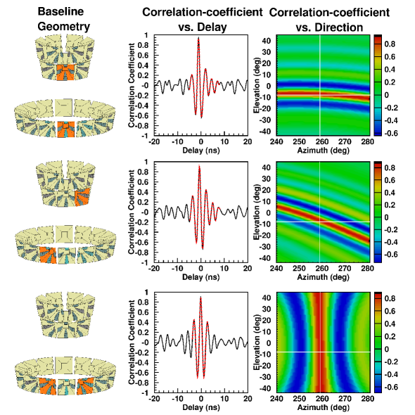
Figure 6 shows the projection of a cross-correlation coefficient from signals incident on a pair of antennas for several orientations. The time-domain fringe pattern is projected to the incident direction space, in payload elevation and azimuth coordinates, and their direction is perpendicular to the baseline vector orientation. The azimuthal resolution is dominated by horizontal baselines while elevation angle resolution is dominated by the vertical baselines with contributions from the diagonal baselines. The fringe width in the incident direction plot is inversely proportional to the separation of the antennas and depends on the frequency content of the signal.
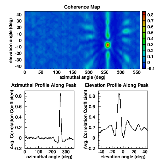
An example of the image formed by the coherence map is shown in Figure 7. The image, formed by the superposition of fringes oriented in various directions, peaks in the direction of incidence of the impulse. Note that although the individual cross-correlation coefficients have sidelobes comparable to the true direction of incidence, their superposition produces a sharp peak, which greatly reduces the possibility of mis-reconstruction and increases the ability to reconstruct the direction of noisy signals.
In general, a windowing strategy is necessary to produce a coherence map and the choice depends on the properties of the antennas as well as the geometric configuration of the array. In the case of ANITA, the coherence map , as shown in Figure 7 and subsequent figures, is based on the symmetry of the array as well as the antenna beam width. The global image is composed of the stitching of 16 images, each with an azimuthal field of view of , centered around each -sector of the payload. All the antennas from four adjacent -sectors ( 5 -sectors in total) are used in the formation of the image.
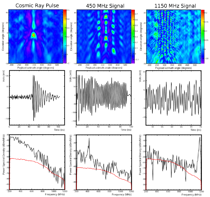
Figure 8 provides examples of the coherence map , coherent waveform sum in the direction of the peak of , and its power spectrum for signals from the ANITA-I flight. The cosmic ray signal, shown on the left, is strong with a clearly defined peak on the coherence map. Although the cosmic ray signal is highly impulsive [26], the coherent waveform sum displays various oscillations due to the low frequency contents of the signal, where the ANITA impulse response is dispersive (see Section 2.1). In the center of Figure 8, a 450 MHz carrier-wave (CW) signal displays a coherence map with multiple lobes of comparable amplitude. The 1150 MHz signal, shown on the right, displays many more lobes of smaller angular size on the coherence map.
In this section we have derived the Adding Interferometer equation for and Cross-Correlation Interferometer equations for and from the coherent waveform sum . Although we primarily use for the ANITA analysis, this is not to say that , , and do not have advantages for certain applications where it makes sense to use them. As we will show in the next section, the ANITA analysis relies heavily on the combination of with the peak of . With the relations between the interferometric quantities presented in this section being well understood, an analysis can be tailored to use each quantity, or combinations of them, as needed for the desired application.
3 Reconstruction of Impulsive Point Sources
The coherence map is a powerful tool not only because it allows for the identification of a point source direction but also because it provides an efficient means to reject thermal noise and weak sources of interference. The coherence map can be combined with the coherent waveform sum and other related quantities from the previous section to provide for more sensitive analysis tools. In this section we discuss point source reconstruction and background rejection. We illustrate the application of the tools developed in this paper with examples from the ANITA analysis.
3.1 Event Reconstruction
The primary means of reconstructing a signal is to identify the peak of the coherence map . The coherent waveform sum provides a means of inspection for the quality of the reconstruction. One can compare the peak of the coherence map to the peak of or as an additional check of the correctness and fidelity of the reconstruction. The individual waveforms should appear aligned, as was shown in Figure 3.
For an interferometric image, such as , the resolution of a point source is proportional to , as prescribed by the Rayleigh criterion, where is the wavelength of the radiation and is the separation between antennas. It is important to distinguish between the resolution of the image, which is the width of the peak, and the reconstruction error, which is the statistical scatter on the location of the peak after repeated measurements. In the case of wideband radio impulses the errors can be significantly better than the resolution estimate provides. The factors that affect the error of the location of the peak, besides the ratio , are the SNR, the bandwidth of the impulse, and the number of antennas observing the signal.
For uncorrelated noise, the error on the source direction is inversely proportional to SNR (see Appendix A). The fact that a wideband impulse does not reside in a single frequency but rather over many bands requires some care in relating the resolution (proportional to ) to the signal to noise ratio. The relation between the SNR of an impulse and the signal-to-noise ratio of its spectral components depends on the spectral shape of the impulse and the noise background. For a digitizer with sampling frequency the frequency resolution is where is the number of samples recorded. For a signal with bandwidth , the number of independent frequency measurements made on the signal is . For a non-dispersive signal with a constant spectral signal to noise ratio (where the signal Fourier amplitude is a constant multiple of the average thermal noise Fourier amplitude for a given frequency range), the time-domain impulse SNR is related to the signal-to-noise ratio of the individual spectral () amplitudes by , where is the bandwidth of the impulse. In this illustrative case, the error on the direction of a wideband impulse is proportional to the , where is the central wavelength and inversely proportional to . See Appendix A for a more rigorous derivation.
The improvement in directional reconstruction errors can be estimated by counting the number of independent measurements contributing to the result. In the paragraph above we discussed the contribution of the number of bands . For an array with antennas, there are independent baselines555The total number of baselines can be represented as linear combinations of a subset of linearly independent baseline vectors.. The number of independent measurements contributing to the directional reconstruction of the signal is the number of independent baselines times the number of independent frequency measurements. For the ANITA antenna geometry, the directional reconstruction error improves approximately by a factor of over the image resolution estimate proportional to . See Appendix A for a more rigorous estimation of the point source impulsive reconstruction errors.
For the ANITA analysis, the coherence map is calculated with pixels. The peak widths of impulsive events for ANITA are typically for elevation and for azimuth (see Figure 7) depending on the frequency contents of the impulse (see Figure 8). The peak widths are consistent with the resolution estimate for the frequencies and baseline lengths involved in making the image. When testing the angular reconstruction errors for point sources with a calibration pulser, the statistical errors are measured to be in elevation and in azimuth [29]. For ANITA, the sampling frequency Gsa/s and the recording window is 256 samples giving MHz. The calibration impulse has a bandwidth MHz. Each pixel in the coherence map image uses 10 antennas. The angular error therefore improves by over the resolution, resulting in an estimated errors of in elevation and in azimuth. The elevation and azimuth errors are consistent with the measured errors of and , respectively.
Both the ANITA-I and ANITA-II data show a clear dependence on angular error with SNR. Figure 9 shows the dependence of angular error on single antenna SNR for the ANITA-II pointing calibration. The quality of the angular reconstruction error can vary by a factor of 2 between the weakest and strongest signals. The comparison between the detected , plotted in Figure 9, and the theoretical used in the discussion above is not straightforward due to various complications such as impulse dispersion (the signal is not a perfect delta-function impulse), the impulse signal and noise spectral varies with frequency, and there are additional error contributions due to clock synchronization and other calibrations. However, the discussion above does provide a reasonably accurate estimate of the pointing error improvement over the image resolution.

3.2 Thermal Noise Rejection
The ANITA data consist of 99% thermal noise events with potentially a few neutrino events expected near the thermal noise threshold. The ANITA analysis is searching for a small signal sample in a large thermal noise background and therefore requires a highly efficient thermal noise filter. This section will discuss how the interferometric quantities developed in this paper were used to successfully obtain a highly sensitive means of rejecting thermal noise.
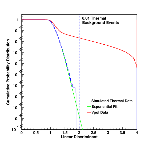
The combined use of the coherence map and the coherently summed waveform provide a complementary handle on thermal noise rejection. Figure 10 shows the peak coherence map value , where is the direction of the peak, plotted against the SNR of . In the case of thermal noise, these quantities become anti-correlated when either of them have a high value. If the total level of coherence fluctuates upward, the peak value of the waveform sum tends to be low. Conversely, if the noise displays a large peak, the correlation, which uses all points in the waveforms, tends to be low. This is an advantageous discriminator of impulsive signals which have a high peak coherence map value and a high summed waveform SNR.

For this purpose we apply a Fisher linear discriminant, in the form of , that combines the values of the peak coherence map and coherently summed waveform SNR . The slope of linear discriminant is chosen so that it is tangential to the contours shown in the thermal noise simulations in Figure 10 while shifts the overall level up and down. The distribution of the linear discriminant value , shown in Figure 11, has an exponential fall-off at the tail. The trend has been extrapolated to set a cut consistent with 0.01 thermal events passing for all of the ANITA-I data set. The value of this discriminant is shown for the all ANITA-I events in the vertically polarized channel. The black dots in Figure 10 show the distribution of 1000 simulated triggered neutrino signals [10] showing that the linear discriminant is a highly efficient filter of thermal noise.
3.3 Radio Frequency Interference
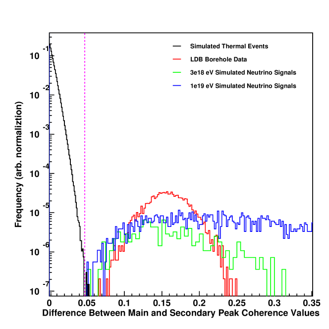
Prior to the pointing analysis, the ANITA data goes through an adaptive notch filter to identify and remove CW peaks from signal spectra of the data. The most common source of mis-reconstruction is the presence of a weak CW signal that has survived the pre-filtering process. Fortunately, such signals have a tendency to produce coherence maps with multiple peaks of similar strength (see the middle panel of Figure 8). We are able to reject this class of events by comparing the difference of the main peak of the coherence map to the second strongest peak. This quantity provides a cut value to reduce the probability of a weak CW signal passing as an event of interest.
Anthropogenic noise is unpredictable and often involves weak CW signals in several bands. For this reason we optimize the level of the cut according to the amount of signal surviving it. Figure 12 shows the distribution of the difference between the first and second peak for calibration signals as well as simulated neutrino signals. The cut is set to preserve all the signals while removing a large portion of weak CW residuals. The thermal event distribution is also plotted showing a sharp exponential drop. We allow some thermal events to pass given that the linear discriminant, discussed in Section 3.2, since the linear discriminant already takes care of any potential thermal contamination in the data set.
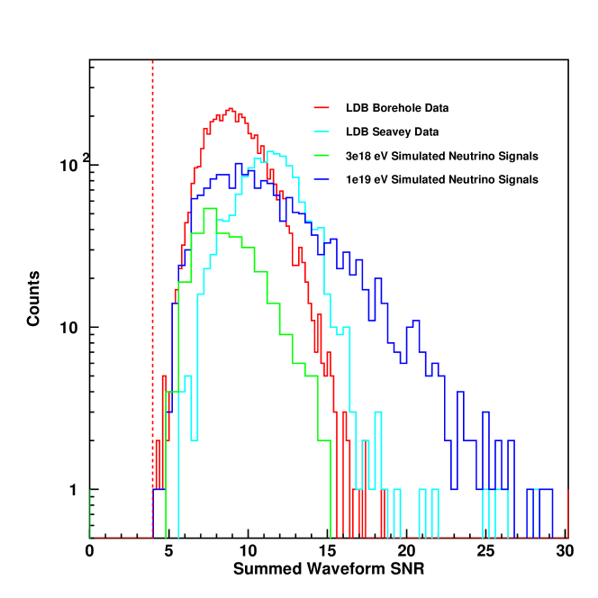
The effect of weak CW interference also manifests itself in the comparison of the peak coherence value versus the SNR of (the maximum peak-to-peak distance of the coherently summed waveform calculated in the direction of peak coherence). The population of events in the data that produce the contours on the region between an SNR of 1 and 3 and coherence values greater than 0.1, in Figure 10, is due weak CW contamination, which results in an increased coherence while not displaying a strong SNR in . The distribution of coherent waveform sum SNR is shown in Figure 13 for calibration signals and simulated data. Cutting data with SNR4 filters out most weak CW interference while retaining signals with 100% efficiency.
4 Identification and Characterization of Weak Signals
If a stationary source is too weak to be detected in a single interferometric image, the images can be stacked to provide a strong detection. This technique can be useful for characterizing known weak sources of noise as well as identifying new ones. We demonstrate the use of averaging interferometric images with short integration times to observe the Sun. We apply a similar technique to producing RF source maps of the Antarctic continent.
4.1 Solar Imaging
The Sun, while a significant thermal source in ANITA’s frequency range, is not distinguishable in a single interferometric image created from ANITA data. Each ANITA interferometric image contains only 100 ns of data. To detect such a source, one must combine many events by averaging the individual interferometric images together. Selection of a coordinate system in which the source of interest is stationary allows the signal to remain constant while the noise averages down, and is essential to this process.
So far, we have plotted the coherence map as a function of payload elevation and azimuth . This is the coordinate system used in Figures 5, 6, 7, and 8. However, we can just as well select another reference coordinate system for the image. For the purpose of imaging the Sun, we use solar azimuth , where corresponds to the location of the Sun. Although at South Polar latitudes the Sun changes elevation angle throughout the day, it is reasonably stationary in the 30 minute time scales used for averaging. Making the coherence map in this coordinate system reduces to recalculating the baseline delays and averaging the cross-correlation coefficients for each baseline to produce the coherence map . Each map, using a 100 ns snapshot in the case of ANITA, will not reveal an image of the Sun. However, the average map over events
| (13) |
where the index runs over all events used in the average, will produce an image given that is large enough.
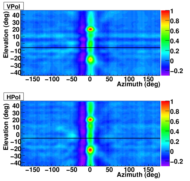
Figure 14 shows an image of the Sun created by averaging together 10,000 ANITA events (1 ms of data, recorded over a 30 minutes period). The image created from the average amplitudes of each pixel clearly reveals the Sun and its surrounding sidelobes. This image shows a peak corresponding to the location of the Sun at 20∘. In addition, the image shows a bright spot consistent with the Sun’s reflection on the ice at -20∘. The reflection is stronger in the horizontally polarized image than the vertically polarized image, as expected from the Fresnel reflection coefficients on the surface of the ice, with index of refraction . Another interesting feature are the horizontal bright lines spanning the full azimuthal field of view. These lines could be due to the horizon where the noise temperature transitions from 270∘ K on the surface to 10∘ K on the sky. No conclusive evidence has been found to distinguish it from a detector artifact and the effect is currently under investigation.
This technique is being further explored for a variety of applications and will be treated in detail in an upcoming publication [36]. The Sun provides a constant source that allows us to monitor the antenna gain calibration throughout the flight. We can also monitor the surface radio reflectivity by comparing the brightness of the Sun and its reflection both in the vertical and horizontal polarizations. This comparison provides a direct measure of the index of refraction of the surface of the ice. Surface roughness estimates are important to the energy determination of reflected ultra-high energy cosmic ray air shower events [26].
4.2 Man-Made RF Activity on the Antarctic Continent
Except for a small fraction of signals expected from ultra-high energy particles, ANITA records two main types of events: first, thermal noise fluctuations that trigger the system comprising 99% of the data and second, anthropogenic signals originating from Antarctic bases, field camps, traverses, and potentially aircraft comprising the remaining 1% of the data. There is, however, some overlap in these events. Some anthropogenic sources can be well below ANITA’s trigger threshold but still present in the thermal noise triggered data. Much like the treatment of the Sun in section 4.1, we are able to make subthreshold maps of the Antarctic continent.
For ANITA-I, a total of 8 M events were collected, making the projection of all coherence maps onto a coordinate system covering Antarctica impractical. However, we can take the peak value and direction of the coherence map for each event and project it onto the Antarctic continent. In the following, we describe the mapping procedure. First, we find the peak direction of the coherence map in payload coordinates , . We then transform the direction to a local East, North, Vertical (ENV) coordinate system to obtain the direction of the peak in , . This involves correcting for payload heading and attitude offsets from vertical [10]. The location of the payload is determined by an on-board global positioning system (GPS) unit reported in Earth-Centered Earth-Fixed (ECEF) Cartesian coordinates. The direction of the peak coherence also needs to be transformed to , . Given the position and direction of the peak coherence, we can propagate the ray to a location on the Antarctic continent. To do this, we bin the continent in Easting, Northing coordinates666Easting and Northing coordinates place the South Pole as the origin with the y-axis (Northing) pointed along longitude line and the x-axis (Easting) pointed along the longitudinal line. in 10 km by 10 km squares. Using an elevation model of the continent [35] we determine the ECEF coordinates () for the center of each bin . We then linearly propagate the ray from () in the direction of , to find the closest bin () consistent with that propagation.
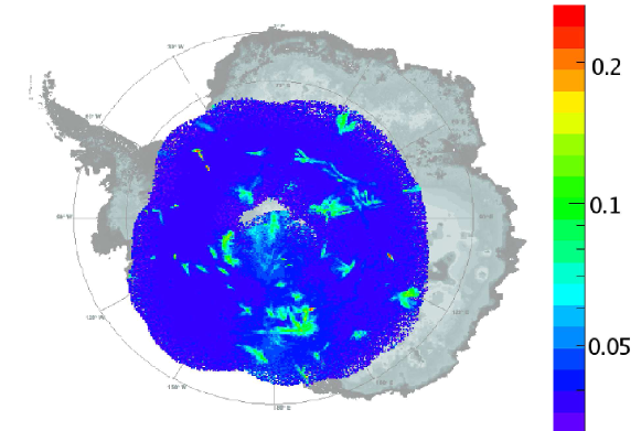
Figure 15 shows the average of the peak coherence values for events projected into each bin on the Antarctic continent for vertically polarized data of all 8 M events from ANITA-I. The blue background is consistent with the thermal noise expectation, while the colored regions indicate hot-spots of anthropogenic activity. Figure 16 shows a similar map made using all 21.2 M events from ANITA-II [29]. More anthropogenic hot-spots were observed with ANITA-II because of the increased exposure and sensitivity of that flight.
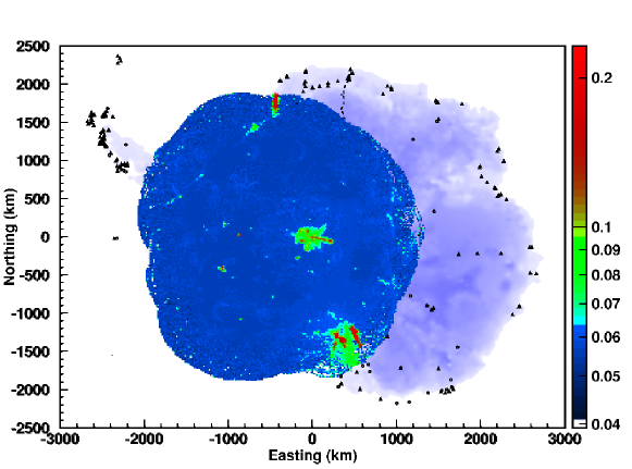
When these maps, made for all the data, are compared to the event clusters passing the thermal noise and CW filters, we find clusters of activity that do not appear in the latter population of events. This indicates that there is potential for a single anthropogenic transient event that could be detected from among the background of sub-threshold signals. We therefore exclude any events from such sites in the final analysis [29]. It is also interesting to note that this technique provides a diagnostic for the radio quiet properties of a given site. If we look at how the events in each bin are distributed in peak coherence, we can determine whether the site is consistent with pure thermal noise or if there is some sub-threshold tail indicating weak anthropogenic activity. We have used this technique for visual inspection and we are currently looking into applying it more formally to the data analysis.
Reliable directional reconstruction of anthropogenic activity was critical to the results of the ANITA-I and ANITA-II ultra-high energy neutrino searches [34, 29]. The criteria for tagging an above threshold event (an event passing the thermal noise and CW filters) as anthropogenic is any one of the following: the event clusters with other above threshold events, the event clusters with a known location of human activity regardless of whether it also clusters with other above threshold events, the event clusters with a local maximum (hot-spot) from Figure 15 for ANITA-I or Figure 16 for ANITA-II which may be formed by purely subthreshold signals. If any of these cases are satisfied the event is rejected. For ANITA-I, one isolated event was identified as a man-made background event by association with a hot-spot formed solely out of subthreshold events. Even though there is a significant amount of human activity on the Antarctic continent, especially as seen by ANITA-II, only 36% of the continent was excluded in the ANITA-II neutrino search analysis due to proximity to anthropogenic events [29]. The blue regions shown in Figures 15 and 16, indicate quiet regions where neutrino candidate signals could be found.
5 Outlook and Conclusions
The interferometric techniques developed for impulsive signals are applicable not only to event reconstruction but also to filtering of thermal noise and radio interference as well as the identification of weak background sources. The methods presented are suited for antenna arrays with digital sampling capabilities, the kind of detector fit for searches of UHE particle impulsive transient radio emission. The applications discussed in this paper are only a subset of the capabilities provided by the interferometric technique and several others are currently under development.
Future applications of the Solar imaging technique include estimation of the surface roughness of the Antarctic ice by comparing the direct and reflected images. This technique can also be applied to a determination of the index of refraction and reflectivity of the Antarctic surface. The analysis of Solar reflections will also provide a measure of surface roughness on the Antarctic continent relevant to the energy determination of ultra-high energy cosmic ray events [36].
The interferometric principles presented in this paper are also being applied towards the development of a new trigger for the third flight of ANITA. The interferometric trigger will continuously digitize data with 3-bit resolution in real-time. The beam-forming can then be performed in real-time using an application-specific integrated circuit or a field-programmable gate array, if the power consumption allows. The development of the interferometric technique for impulsive transients applied to hardware algorithms will be treated in a future publication.
The application of interferometric imaging to impulsive signals has proved to be a powerful technique. It is by no means limited to what has been presented in this paper and it will continue to be exploited in future efforts for the radio detection of ultra-high energy particles.
6 Acknowledgments
We thank the National Aeronautics and Space Administration, the National Science Foundation Office of Polar Programs, the Department of Energy Office of Science HEP Division, the UK Science and Technology Facilities Council, the National Science Council in Taiwan ROC, and especially the staff of the Columbia Scientific Balloon Facility. A. Romero-Wolf would like to thank NASA (NESSF Grant NNX07AO05H) for support for this work. A.G. Vieregg would like to thank NASA (NESSF Grant 09-Astro-09F-0008) and the National Science Foundation (Grant No. ANT-110355). Copyright 2013. All rights reserved.
Appendix A Statistical Pointing Error Estimation
A.1 Probability Density Function and Likelihood Estimator
In this appendix we estimate the pointing errors from a likelihood estimator approach. Following [33], the probability density function , for the amplitude and phase of a phasor , resulting from the sum of a number of random contributions large enough to satisfy the central limit theorem, is
| (14) |
where is the noise level. The probability density function has units of inverse amplitude times inverse radians and is written as to make it explicit that it is a differential probability density. Expressed in terms of the real and imaginary parts of , the probability density function is a bivariate Gaussian distribution
| (15) |
In the presence of a signal phasor with with amplitude s and phase , in a noise background the probability density function becomes
| (16) |
The likelihood function associated with the probability density function described is
| (17) |
A.2 Likelihood Estimator of a Digitized Signal Observed by an Array of Antennas
Let’s assume we have an array of antennas indexed by . If the signal at each antenna is digitized with sampling frequency with samples, then the frequency resolution is . For uncorrelated noise, each frequency bin of width is an independent measurement indexed by . For an array of antennas with effective height observing an electric field (in one polarization), the antenna signal can be represented as where is the geometrical delay of the signal . For simplicity we have assumed that the overall electric field phase is at zero degrees and that the antenna effective height does not affect the phase other than by the geometric delay. Adding these dependencies is straightforward but we want to keep the following derivation as simple as possible.
Using Equation 17, the likelihood function for the array is given by
| (18) |
where and are the measured real and imaginary parts for the phasors of each antenna indexed by at each frequency indexed by . The sum over frequencies has independent contributions for a real digitized signal.
The error for is estimated from the second derivative of the maximum likelihood estimator. The first derivative with respect to gives
| (19) |
The second derivative with respect to gives
| (20) |
In the limit where the data approaches the modeled values and
| (21) |
Note that is the signal to noise ratio () at the antenna at frequency bin corresponding to .
For the purpose of illustration, let us assume we have a collinear array so that , where is the distance to the origin and is the angle between and . Let us also assume that only one frequency bin has . The expression then becomes
| (22) |
We estimate the angular error using the relation . Note that the error is not arbitrarily small given the choice of a distant origin. If this is the case, all the angles will be small compensating for the choice of large ’s. Let us assume that a signal is incident orthogonal to the collinear array axis. If we set the origin at the location of one of the antennas, say the th one, then its contribution drops out of the sum because . Then we have
| (23) |
Assuming that is the same for each antenna
| (24) |
For the ANITA geometry, the antenna beam pattern is wide enough so that there are several vertical baseline pairs contributing to the elevation error. In this case there is a fixed vertical distance giving an improvement of roughly . The error can be calculated more rigorously using the effective heights of the antenna which make the channel to channel vary.
In general, the digitization with records is sensitive to independent frequencies. Then we have
| (25) |
Let us assume that there is a relatively large number of frequency bins , spanning indices to , for which the signal to noise ratio is constant and non-zero. The error estimate is
| (26) |
Let us evaluate . For a digitized signal with we have . For a large number of frequency bins the sum results in . Factorization gives . The first term is the number of frequencies with non-zero SNR . The second term gives for the central frequency Together these give
| (27) |
Thus, the direction error is reduced by a factor of . Intuitively, this result can be interpreted as each independent frequency providing an independent interferometric estimate of the incident angle .
A.3 Likelihood Estimator of an Interferometric Array
A similar likelihood analysis can be performed on the cross-correlation phasor defined as the product of two phasors. The cross-correlation phasor for a signal incident on the interferometric array is given by . The advantage of this approach is that any ambiguities due to choice of coordinate system vanish, since only delay differences between antenna pairs are counted. However, the estimation of the cross-correlation phasor noise is non-trivial and the accounting of independent contributions has additional complications. A maximum likelihood analysis technique along these lines has been developed for interferometric observations of the cosmic microwave background [37]. This approach is currently being developed as a potential improvement on the interferometric analysis presented on this paper and for a more rigorous accounting of errors. This will be the subject of a future publication.
References
- [1] G. A. Askaryan, JETP 14, 441 (1962); JETP 21, 658 (1965).
- [2] D. Saltzberg et al., Phys. Rev. Lett., 86, 2802, (2001).
- [3] E. Zas, F. Halzen, and T. Stanev, Phys. Rev. D 45, 362-376 (1992).
- [4] P.W. Gorham et al., Phys.Rev. D, 72, 023002, (2005)
- [5] ANITA Collaboration: P.W. Gorham, et al., Phys. Rev. Lett. 99, 171101, (2007).
- [6] I. Kravchenko, et al., Phys. Rev. D 73, 082002, (2006).
- [7] P. Allison, et al., Astropart. Phys. 35, 457–477, (2012).
- [8] P. W. Gorham, et al., Phys. Rev. Lett. 93, 041101 (2004)
- [9] C. W. James, et al., Phys. Rev. D, 81, 042003 (2010)
- [10] ANITA Collaboration: P.W. Gorham et al., Astropart. Phys. 32, 10-41, (2009)
- [11] Falcke, H. and Gorham, P., Astropart. Phys. 19, 477-494 (2003).
- [12] Suprun, D. A., Gorham, P. W., and Rosner, J. L., Astropart. Phys. 20 157-168, (2003).
- [13] Jelley, J. V. et al., Nature 205, 327-328 (1965).
- [14] Porter, N. A., Long, C. D., McBreen, B., Murnaghan, D. J. B. and Weekes, T. C., Phys. Lett. 19, 415-417 (1965).
- [15] Vernov, S. N., Abrosimov, A. T., Volovik, V. D., Zalyubovskii, I. I. and Khristiansen, G. B., Pis’ma v ZhETF 5, 157-162 (1967). [Sov. Phys. JETP Letters 5, 126-130 (1967)]
- [16] Barker, P. R., Hazen, W. E., and Hendel, A. Z., Phys. Rev. Lett. 18, 51-54 (1967).
- [17] Fegan, D. J. and Slevin, P. J., Nature 217, 440-441 (1968).
- [18] Hazen, W. E., Hendel, A. Z., Smith, H., and Shah N. J., Phys. Rev. Lett. 22, 35-37 (1969).
- [19] Hazen, W. E., Hendel, A. Z., Smith, H., and Shah N. J., 24, 476-479 (1970).
- [20] Spencer, R. E., Nature 222, 460-461 (1969).
- [21] Fegan, D. J. and Jennings, D. M., Nature 223, 722-723 (1969).
- [22] Allan, H. R., Progress in Elementary Particles and Cosmic Ray Physics, 10, edited by Wilson, J. G. and Wouthuysen S. G. (North-Holland, Amsterdam, 1971), 171-304, and references therein.
- [23] Ardouin, D. et al., Astropart. Phys. 31, 192-200 (2009).
- [24] Nehls, S. et al., Nucl. Instrum. Meth. A589, 350-361 (2008).
- [25] LOPES Collaboration, W. D. Apel et al., Astropart. Phys. 32, 294-303 (2010).
- [26] ANITA Collaboration: S. Hoover et al., Phys. Rev. Lett. 105, 151101 (2010).
- [27] A.R. Thompson, J.M. Moran, G.W. Swenson, Interferometry and Synthesis in Radio Astronomy, John Wiley & Sons, 1986
- [28] O.J. Sovers, J.L. Fanselow, C.S. Jacobs, Rev. Mod. Phys. 70, 1393-1454 (1998)
- [29] ANITA Collaboration: P.W. Gorham et al., Phys. Rev. D 82, 022004 (2010); Phys. Rev. D 85, 049901(E) (2012)
- [30] Falcke H., et al., Nature 435, 313-316 (2005)
- [31] Miočinović, P., et al., Phys. Rev. D 74, 043002 (2006)
- [32] J. Alvarez-Muñiz, A. Romero-Wolf, and E. Zas, Phys. Rev. D 84, 103003 (2011)
- [33] J. W. Goodman, Statistical Optics, John Wiley and Sons, 1985.
- [34] ANITA Collaboration: P.W. Gorham et al., Phys. Rev. Lett. 103 051103, (2009)
- [35] Liu, H., Jezek, K., Li, B., and Zhao, Z.. 2001. Boulder, CO: National Snow and Ice Data Center. Digital media
- [36] D. Besson et al.,“Antarctic Radio Frequency Albedo and Implications for Cosmic Ray Reconstruction”, arXiv 1301.4423 (2013)
- [37] L. Zhang, A. Karacki, P. Sutter et al., “Maximum Likelihood Analysis of Systematic Errors in the Interferometric Observations of the Cosmic Microwave Background” , http://arxiv.org/abs/1209.2676 (2012)