On Integrating Deductive Synthesis and Verification Systems

Abstract

We describe techniques for synthesis and verification of recursive functional programs over unbounded domains. Our techniques build on top of an algorithm for satisfiability modulo recursive functions, a framework for deductive synthesis, and complete synthesis procedures for algebraic data types. We present new counterexample-guided algorithms for constructing verified programs. We have implemented these algorithms in an integrated environment for interactive verification and synthesis from relational specifications. Our system was able to synthesize a number of useful recursive functions that manipulate unbounded numbers and data structures.

1 Introduction

Software construction is a difficult problem-solving activity. It remains a largely manual effort today, despite significant progress in software development environments and tools. The development becomes even more difficult when the goal is to deliver verified software, which must satisfy specifications such as assertions, pre-conditions, and post-conditions.

We believe that quick feedback and error reports are essential for practical verification. Verifying programs after they have been developed is extremely time-consuming Leinenbach and Santen [2009]; Klein et al. [2009] and it is difficult to argue its cost-effectiveness. Our research therefore explores approaches that support integrated software construction and verification. An important aspect of such approaches are modular verification techniques which can check that a function conforms to its local specification. In such approach, the verification of an individual function against its specification can start before the entire software system is completed, so tools can provide rapid feedback that allows specifications and implementations to be developed simultaneously. Quoting Barnett et al. [2011], who report on the experience with Spec#,

“If verification ever makes it into the daily rhythm of mainstream programming, it will be through a design-time interface providing online verification.”

We choose a functional language as the core language for the development of verified software. Functional languages strike an appealing balance between executability and verifiability, predicted already in McCarthy [1960]. Although the problem of delivering verified software has been explored through a number of different approaches, in a number of successful cases the development relies heavily on a functional language. In some cases Klein et al. [2009] the researchers have even written the entire software system once in a functional language for verifiability, and once in a lower-level language for execution efficiency.

Based on the ideas of suitability of a functional paradigm and the importance of rapid feedback, we have developed a verifier that quickly detects errors in functional programs and reports concrete counterexamples, but can also prove the correctness of programs Suter [2012]; Suter et al. [2010, 2011]. Furthermore, we have integrated such countexample-generating verifier into a web-browser-based IDE, resulting in a tool for convenient development of verified functional programs. This verifier is the starting point of the tool we present in this paper.

Moving beyond verification, we believe that a productive development of verified software requires techniques for synthesis from specifications. Specifications in terms of properties generalize existing declarative programming language paradigms by allowing the statement of constraints between inputs and outputs as opposed to always specifying outputs as functions of inputs Jaffar and Lassez [1987]; Köksal et al. [2012]. Unlike deterministic specifications, constraints can be composed using conjunctions, which enables description of the problem as a combination of orthogonal requirements.

This paper introduces synthesis algorithms, techniques and tools that integrate synthesis into the development process for functional program. We present a synthesizer that can construct the bodies of functions starting solely from their postconditions. The programs that our synthesizer produces typically manipulate unbounded data types, such as algebraic data types and unbounded integers. Thanks to the use of deductive synthesis and the availability of a verifier, when the synthesizer succeeds, the generated code is guaranteed to be correct for all possible input values.

Our synthesizer uses specifications as the description of the synthesis problems. While it could additionally accept input/output examples to illustrate the desired functionality, we view such illustration as a special form of input/output relation: whereas input/output examples correspond to tests and provide a description of a finite portion of the desired functionality, we primarily focus on symbolic descriptions, which ensure the desired behavior over an arbitrarily large or even infinite domain. From such descriptions, our synthesizer can automatically generate input/output examples when needed, but can also use them and transform them directly into executable code.

A notable degree of automation in our synthesizer comes from synthesis procedures Kuncak et al. [2010, 2012]; Jacobs et al. [2013], which compile specification fragments expressed in decidable logics. Our work is the first implementation of the synthesis procedure for algebraic data types Suter [2012].

Note however, that, to capture a variety of scenarios in software development, we also support the general problem of synthesis of Turing-complete programs. The result is a framework for cost-guided application of deductive synthesis rules, which decompose the problems into subproblems.

Our synthesizer tightly cooperates with the underlying verifier, which allows it to achieve orders of magnitude better performance than using simpler generate-and-test approaches. Techniques we use include symbolic transformation based on synthesis procedures, as well as synthesis of recursive functions using counterexample-guided strategies. We have evaluated a number of system architectures and trade-offs between symbolic and concrete reasoning in our implementation and arrived at an implementation that is successful despite the large space of possible programs.

We believe that we have achieved a new level of automation for a broad domain of recursive functional programs. We consider a particular strength of our system that it can synthesize code that satisfies a given relational specification for all values of inputs, and not only given input/output pairs.

Despite aiming at a high automation level, we are aware that any general-purpose automated synthesis procedure will ultimately face limitations of scalability and the ability to control the development process. We deployed the synthesis algorithm as an interactive assistance that allows the developer to interleave manual and automated development steps. In our system, the developer can decompose a function and leave the subcomponents to the synthesizer, or, conversely, the synthesizer can decompose the problem, solve some of the subproblems, and leave the remaining open cases for the developer. To facilitate such synergy, we deploy an anytime synthesis procedure, which maintains a ranked list of current problem decompositions. The user can interrupt the synthesizer at any time to display the current solution and continue manual development. This is possible thanks to the fact that synthesis problems and specification problems are both expressed in a unified language based on the construct resembling non-deterministic choice.

1.1 Contributions

The overall contribution of this paper is an integrated synthesis and development system for automated and interactive development of verified programs. A number of techniques from deductive and inductive reasoning need to come together to make such system usable.

Verifier.

Our automated verification environment is the enabler of synthesis. We use SMT solvers, specifically Z3 de Moura and Bjørner [2008], and a fair function unfolding strategy that is effective for sufficiently surjective abstractions Suter et al. [2010, 2011]. We have achieved substantial speed-ups of this technique for satisfiable constraints through the use of code generation and fair enumeration of structured values. The improvements in verification and falsification have transferred to the improvements in synthesis times.

Implemented synthesis framework.

We developed a deductive synthesis framework that can accept a given set of synthesis rules and applies them according to a cost function. The framework accepts 1) a path conditions that encode program context, and 2) a relational specifications. It returns the function from inputs to outputs as a solution, as well as any necessary strengthening of the precondition needed for the function to satisfy the specification. We have deployed the framework in a web-browser-based environment with continuous compilation and the ability to interrupt the synthesis to obtain a partial solution in the form of a new program with a possibly simpler synthesis problem.

Data type synthesis.

Within the above framework we have implemented rules for synthesis of algebraic data type equations and disequations Suter [2012], as well as a number of general rules for decomposing specifications based on their logical structure or case splits on commonly useful conditions. We have developed program simplification techniques that post-process the generated code and make it more readable.

Support for recursion schemas and symbolic term generators.

One of the main strengths in our framework is a new form of counterexample-guided synthesis that arises from a combination of several rules.

• A set of built-in recursion schemas can solve a problem by generating a fresh recursive function. To ensure well-foundedness we have extended our verifier with termination checking, and therefore generate only terminating function calls in this rule.

• To generate bodies of functions, we have symbolic term generators that systematically generate well-typed programs built from selected set of operators (such as algebraic data type constructors and selectors). To test candidate terms against specifications we use the Leon’s verifier. To speed up this search, the rule accumulates previously found counterexamples. Moreover, to quickly bootstrap the set of examples it uses systematic generators that can enumerate in a fair way any finite prefix of a countable set of structured values. The falsification of generated bodies is done by direct execution of code. For this purpose, we have developed a lightweight compiler for our subset of Scala into bytecodes, replacing many constraint reasoning steps by code execution.

Function generation by condition abduction.

We also present and evaluate an alternative counterexample-guided rule tailored towards synthesis of recursive conditional functions, with the following characteristics.

• Instead of specialized term evaluators, the rule uses a general expression enumerator based on generating all expressions of a given type Gvero et al. [2013]. This results in a broad coverage of expressions that the rule can synthesize. It uses a new lazy enumeration algorithm for such expressions with polynomial-time access to the next term to enumerate Kuraj [2013]. Similarly to the previous rule, it filters well-typed expressions using counterexamples generated from specifications and previous function candidates, as well as based on structured value genererators.

• The most distinctive aspect of this rule is the handling of conditional expressions. The expressions are synthesized by collecting relevant terms that satisfy a notable number of derived test inputs, and then trying to synthesize predicates that imply the correctness of candidate terms. This is an alternative to relying on existing rules to perform splitting on simple conditions. Effectively, the additional rule performs abduction of conditions until it covers the entire input space with a partition of conditions, where each partition is associated with a term.

Evaluation.

We evaluate the current reach of our synthesizer in fully automated mode by synthesizing functions such as those that merge, partition, and sort lists of objects, where lists are defined using a general mechanism for algebraic data types. This paper presents a description of all the above techniques and a snapshot of our results. We believe that the individual techniques are interesting by themselves, but we also believe that having a system that combines them is essential to understand the potential of these techniques in addressing the difficult problem as synthesis. To gain full experience of the feeling of such development process, we therefore invite the reader to explore the system themselves.

2 Interactive Synthesis and Verification in the Leon System

We start by illustrating through a series of examples how developers can leverage our system to write programs that are correct by construction.

Unary numerals.

As a first example, we will consider tasks related to Unary numerals. While these examples are simple in nature, they illustrate some very important points. In particular, they show how, using a combination of verification and synthesis, one can program functions manipulating data types in one representation while specifying the operations using an abstract view.

Consider a standard definition of unary numerals as a recursive data type, with a base case “zero” and a “successor” constructor.

⬇

sealed abstract class Num

case object Z extends Num

case class S(pred: Num) extends Num

Because it is more convenient to think of these numerals in term of their integer value, we can define an abstraction function that computes it:

⬇

def value(n:Num) : Int = (n match {

case Z $\Rightarrow$ 0

case S(p) $\Rightarrow$ 1 + value(p)

}) ensuring (_ $\geq$ 0)

The ensuring clause is Scala notation for a postcondition Odersky [2010]. These postconditions are defined by an anonymous function, whose single argument denotes the result of the function. The underscore notation is a shorthand for x $\Rightarrow$ x $\geq$ 0, so this annotation simply specifies that the integer representation of a unary numeral is never negative, and Leon instantly proves this simple verification condition.

Using our (verified) abstraction function, we can start specifying operations on unary numerals. Consider for instance the addition operation. Its contract in terms of the value function is clear, so we can write it as:

⬇

def add(x : Num, y : Num) : Num = choose { (r: Num) $\Rightarrow$

value(r) == value(x) + value(y)

}

Here, choose is a special function defined by Leon to represent a computation that needs to be synthesized. Similarly to the postcondition, it is defined by an anonymous functions whose result represents the desired output. Contrary to postconditions, though, the function (or synthesis predicate) can admit multiple arguments, in which case the synthesized program should return a tuple of values of the appropriate types.

Upon invocation of the Leon synthesis component, the following recursive implementation is derived:

⬇

def add(x : Num, y : Num) : Num = (x match {

case Z $\Rightarrow$ y

case S(p) $\Rightarrow$ add(p, S(y))

}) ensuring(r $\Rightarrow$ value(r) == value(x) + value(y))

We can continue expanding on these results, and define a synthesis predicate for multiplication:

⬇

def mult(x : Num, y : Num) : Num = choose { (r: Num) $\Rightarrow$

value(r) == value(x) * value(y)

}

Leveraging the previous results for add, our synthesis algorithm derives the following program:

⬇

def mult(x : Num, y : Num) : Num = (x match {

case Z $\Rightarrow$ Z

case S(p) $\Rightarrow$ add(y, mult(p, y))

}) ensuring(r $\Rightarrow$ value(r) == value(x) * value(y))

Both functions are generated within three seconds.

List manipulation.

We believe this rapid feedback is mandatory when developing from specifications. One reason is that, since contracts are typically partial, results obtained from under-specifications can be remote from the desired output. Thus, a desirable strategy is to rapidly iterate and refine specifications until the output matches the expectations.

As an example, we will consider the task of synthesizing the split function necessary in merge sort. We start from a standard recursive definition of lists, and we assume the existence of recursive functions computing their size (as a non-negative integer), and their content (as a set of integers).

⬇

sealed abstract class List

case class Cons(head: Int, tail: List) extends List

case object Nil extends List

def size(lst : List) : Int = $\ldots$

def content(lst : List) : Set[Int] = $\ldots$

As a first attempt to synthesize split, we try the following specification:

⬇

def split(lst : List) : (List,List) = choose { (r : (List,List)) $\Rightarrow$

content(lst) == content(r._1) ++ content(r._2)

}

Leon instantly generates the following function which, while it satisfies the contract, is not particularly useful:

⬇

def split(lst : List) : (List,List) = (lst, Nil)

To avoid getting a single list with an empty one, we can refine the specification by enforcing that the sizes of the resulting lists should not differ by more than one:

⬇

def split(lst : List) : (List,List) = choose { (r : (List,List)) $\Rightarrow$

content(lst) == content(r._1) ++ content(r._2)

&& abs(size(r._1)-size(r._2)) $\leq$ 1

}

Again, Leon instantly generates a correct, useless, program:

⬇

def split(lst : List) : (List,List) = (lst, lst)

We can further refine the specification by stating that the sum of the sizes of the two lists should match the size of the input one:

⬇

def split(lst : List) : (List,List) = choose { (r : (List,List)) $\Rightarrow$

content(lst) == content(r._1) ++ content(r._2)

&& abs(size(r._1) - size(r._2)) $\leq$ 1

&& (size(r._1) + size(r._2)) == size(lst)

}

We then finally obtain a useful split function:

⬇

def split(lst: List): (List, List) = lst match {

case Nil $\Rightarrow$ (Nil, Nil)

case Cons(h, Nil) $\Rightarrow$ (Nil, Cons(h, Nil))

case Cons(h1, Cons(h2, t2)) $\Rightarrow$

val r = split(t2)

(Cons(h1, r._1), Cons(h2, r._2))

}

We observe that in this programming style, users can write (or generate) code by conjoining orthogonal requirements, such as constraints on the sizes and contents, which are only indirectly related. The rapid feedback make it possible to go through multiple candidates rapidly, strengthening the specification as required.

Sorting.

A typical example of a task that is easier to specify than to implement is sorting. We conclude this overview of Leon’s synthesis capabilities by showing how to derive an insertion sorting algorithm. We start from the straightforward definition of isSorted, a function that checks whether a list is sorted:

⬇

def isSorted(lst : lst) : Boolean = lst match {

case Nil $\Rightarrow$ true

case Cons(_, Nil) $\Rightarrow$ true

case Cons(x1, xs @ Cons(x2, _)) $\Rightarrow$ x1 $\leq$ x2 && isSorted(xs)

}

Using this function, the problem of sorting can be stated as simply as:

⬇

def sort(lst : List): List = choose { (r: List) $\Rightarrow$

isSorted(r) && content(r) == content(lst)

}

To achieve this goal, we start by specifying the helper function insertSorted:

⬇

def insertSorted(lst : List, v: Int): List = {

require(isSorted(lst))

choose { (r: List) $\Rightarrow$

isSorted(r) && content(r) == content(lst) ++ Set(v)

}

}

From this, Leon generates the following solution:

⬇

def insertSorted(lst: List, v: Int): List = {

require(isSorted(lst))

lst match {

case Nil $\Rightarrow$ Cons(v, Nil)

case Cons(h, tail) $\Rightarrow$

val r = insertSorted(t, v)

if (v > h) Cons(h, r)

else if (h == v) r

else Cons(v, Cons(h, t))

}

With the help of this insertion function, we can proceed to synthesizing sort with the simple specification mentioned above. Within five seconds, Leon generates the following implementation of insertion sort:

⬇

def sort(lst : List): List = lst match {

case Nil $\Rightarrow$ Nil

case Cons(h, t) $\Rightarrow$ insertSorted(sort(t), h)

}

3 The Leon Verifier

The results presented in this paper focus on the synthesis component of Leon. The language of Leon is a subset of Scala, as illustrated through the examples of Section 2. Besides integers and user-defined recursive data types, Leon supports booleans, sets and maps.

Solver algorithm.

At the core of Leon is an algorithm to reason about formulas that include user-defined recursive functions, such as size, content, and isSorted in Section 2. The algorithm proceeds by iteratively examining longer and longer execution traces through the recursive functions. It alternates between an over-approximation of the executions, where only unsatisfiability results can be trusted, and an under-approximation, where only satisfiability results can be concluded. The status of each approximation is checked using the state-of-the-art SMT solver Z3 from Microsoft Research de Moura and Bjørner [2008]. The algorithm is a semi-decision procedure, meaning that it is theoretically complete for counterexamples: if a formula is satisfiable, Leon will eventually produce a model Suter et al. [2011]. Additionally, the algorithm works as a decision procedure for a certain class of formulas Suter et al. [2010].

In the past, we have used this core algorithm in the context of verification Suter et al. [2011], but also as part of an experiment in providing run-time support for declarative programming using constructs similar to choose Köksal et al. [2012]. We have in both cases found the performance in finding models to be suitable for the task at hand.

Throughout this paper, we will assume the existence of an algorithm for deciding formulas containing arbitrary recursive functions. Whenever completeness is an issue, we will mention it and describe the steps to be taken in case of, e.g. timeout.

Compilation-based evaluator.

Another component of Leon on which we rely in this paper is an interpreter based on on-the-fly compilation to the JVM. Function definitions are typically compiled once and for all, and can therefore be optimized by the JIT compiler. This component is used during the search in the core algorithm, to validate models and to sometimes optimistically obtain counterexamples. We use it to quickly reject candidate programs during synthesis (see sections 6 and 7).

Ground term generator.

Our system also leverages Leon’s generator of ground terms and its associated model finder. Based on a generate-and-test approach, it can generate small models for formulas by rapidly and fairly enumerating values of any type. For instance, enumerating Lists will produce a stream of values Nil(), Cons(0, Nil()), Cons(0, Cons(0, Nil())), Cons(1,Nil()), …

4 Deductive Synthesis Framework

The approach to synthesis we follow in this paper is to derive programs by a succession of independently validated steps. In this section, we briefly describe the formal reasoning behind these constructive steps and provide some illustrative examples. A more extended exposition of this formal framework is available in Jacobs et al. [2013].

4.1 Synthesis Problems

A synthesis problem is given by a predicate describing a desired relation between a set of input and a set of output variables, as well as the context (program point) at which the synthesis problem appears. We represent such a problem as a quadruple

$$\left\llbracket\bar{a}\ \left\langle\Pi\rhd\phi\right\rangle\ \bar{x}\right\rrbracket$$

where:

• $\bar{a}$ denotes the set of input variables,

• $\bar{x}$ denotes the set of output variables,

• $\phi$ is the synthesis predicate, and

• $\Pi$ is the path condition to the synthesis problem.

The free variables of $\phi$ must be a subset of $\bar{a}\cup\bar{x}$. The path condition denotes a property that holds for input at the program point where synthesis is to be performed, and the free variables of $\Pi$ should therefore be a subset of $\bar{a}$.

As an example, consider the following call to choose:

⬇

def f(a : Int) : Int = {

if(a $\geq$ 0) {

choose((x : Int) $\Rightarrow$ x $\geq$ 0 && a + x $\leq$ 5)

} else $\ldots$

}

The representation of the corresponding synthesis problem is:

$$\left\llbracket a\ \left\langle a\geq 0\rhd x\geq 0\land a+x\leq 5\right\rangle\ x\right\rrbracket$$ (1)

4.2 Synthesis Solutions

We represent a solution to a synthesis problem as a pair

$$\langle{P}\mid{\bar{T}}\rangle$$

where:

• $P$ is the precondition, and

• $\bar{T}$ is the program term.

The free variables of both $P$ and $\bar{T}$ must range over $\bar{a}$. The intuition is that, whenever the path condition and the precondition are satisfied, evaluating $\phi[\bar{x}\mapsto\bar{T}]$ should evaluate to $\mathsf{true}$, i.e. $\bar{T}$ are realizers for a solution to $\bar{x}$ in $\phi$ given the inputs $\bar{a}$. Furthermore, for a solution to be as general as possible, the precondition must be as weak as possible.

Formally, for such a pair to be a solution to a synthesis problem, denoted as

$$\left\llbracket\bar{a}\ \left\langle\Pi\rhd\phi\right\rangle\ \bar{x}\right\rrbracket\vdash\langle{P}\mid{\bar{T}}\rangle$$

the following two properties must hold:

• Relation refinement:

  $$\Pi\land P\models\phi[\bar{x}\mapsto\bar{T}]$$

  This property states that whenever the path- and precondition hold, the program $\bar{T}$ can be used to generate values for the output variables $\bar{x}$ such that the predicate $\phi$ is satisfied.

• Domain preservation:

  $$\Pi\land(\exists\bar{x}:~{}\phi)\models P$$

  This property states that the precondition $P$ cannot exclude inputs for which an output would exist such that $\phi$ is satisfied.

As an example, a valid solution to the synthesis problem (1) is given by:

$$\langle{a\leq 5}\mid{0}\rangle$$

The precondition $a\leq 5$ characterizes exactly the input values for which a solution exists, and for all such values, the constant $0$ is a valid solution term for $x$. Note that the solution is in general not unique; alternative solutions for this particular problem include for instance $\langle{a\leq 5}\mid{5-a}\rangle$, or $\langle{a\leq 5}\mid{\mathsf{if(}a<5\mathsf{)~{}}a+1\mathsf{~{}else~{}}0}\rangle$.

A note on path conditions.

Strictly speaking, the inclusion of the path condition does not add expressive power to the representation of synthesis problems. One can easily verify that the space of solution terms for $\left\llbracket\bar{a}\ \left\langle\Pi\rhd\phi\right\rangle\ \bar{x}\right\rrbracket$ is isomorphic to the one for $\left\llbracket\bar{a}\ \left\langle\mathsf{true}\rhd\Pi\land\phi\right\rangle\ \bar{x}\right\rrbracket$. In the latter case, the path condition $\Pi$, is simply included in the precondition of the solution. On the other hand, from the definition it follows that if $\langle{P}\mid{\bar{T}}\rangle$ is a solution and $\Pi\land P$ is equivalent to $\Pi\land P^{\prime}$ then $\langle{P^{\prime}}\mid{\bar{T}}\rangle$ is also a solution to the synthesis problem. We can let, $P^{\prime}$ be, for example, $\Pi\land P$, or, as another extreme, $\Pi\rightarrow P$. We have therefore found it convenient in the implementation to explicitly keep track of the path conditions and allow freedom in the representation of the returned precondition $P$.

4.3 Inference Rules for Synthesis

One-point $$\displaystyle{\hbox{\hskip 91.4129pt\vbox{\hbox{\hskip-91.4129pt\hbox{\hbox{$\displaystyle\displaystyle\left\llbracket\bar{a}\ \left\langle\Pi\rhd\phi[x_{0}\mapsto t]\right\rangle\ \bar{x}\right\rrbracket\vdash\langle{P}\mid{\bar{T}}\rangle\qquad x_{0}\notin\text{vars}(t)$}}}\vbox{}}}\over\hbox{\hskip 100.48926pt\vbox{\vbox{}\hbox{\hskip-100.48924pt\hbox{\hbox{$\displaystyle\displaystyle\left\llbracket\bar{a}\ \left\langle\Pi\rhd x_{0}=t\land\phi\right\rangle\ x_{0}\mathop{,}\bar{x}\right\rrbracket\vdash\langle{P}\mid{\text{{val}}\ \bar{x}\colonequals\bar{T}\text{{;}}\ (t\mathop{,}\bar{x})}\rangle$}}}}}} \displaystyle{\hbox{\hskip 53.08334pt\vbox{\hbox{\hskip-53.08334pt\hbox{\hbox{$\displaystyle\displaystyle\mathcal{M}\models\phi\qquad\text{vars}(\phi)\cap\bar{a}=\emptyset$}}}\vbox{}}}\over\hbox{\hskip 55.77087pt\vbox{\vbox{}\hbox{\hskip-55.77087pt\hbox{\hbox{$\displaystyle\displaystyle\left\llbracket\bar{a}\ \left\langle\Pi\rhd\phi\right\rangle\ \bar{x}\right\rrbracket\vdash\langle{\mathsf{true}}\mid{\mathcal{M}}\rangle$}}}}}} \displaystyle{\hbox{\hskip 129.69415pt\vbox{\hbox{\hskip-129.69415pt\hbox{\hbox{$\displaystyle\displaystyle\left\llbracket\bar{a}\ \left\langle\Pi\rhd\phi_{1}\right\rangle\ \bar{x}\right\rrbracket\vdash\langle{P_{1}}\mid{\bar{T}_{1}}\rangle\qquad\left\llbracket\bar{a}\ \left\langle\Pi\land\neg P_{1}\rhd\phi_{2}\right\rangle\ \bar{x}\right\rrbracket\vdash\langle{P_{2}}\mid{\bar{T}_{2}}\rangle$}}}\vbox{}}}\over\hbox{\hskip 110.27751pt\vbox{\vbox{}\hbox{\hskip-110.2775pt\hbox{\hbox{$\displaystyle\displaystyle\left\llbracket\bar{a}\ \left\langle\Pi\rhd\phi_{1}\lor\phi_{2}\right\rangle\ \bar{x}\right\rrbracket\vdash\langle{P_{1}\lor P_{2}}\mid{\text{{if(}}P_{1}\text{{) \{}}\bar{T}_{1}\text{{\} else \{}}\bar{T}_{2}\text{{\}}}}\rangle$}}}}}} \displaystyle{\hbox{\hskip 172.2795pt\vbox{\hbox{\hskip-172.27948pt\hbox{\hbox{$\displaystyle\displaystyle(\Pi_{1}\land P)\implies\Pi_{2}\qquad\Pi_{2}[a_{0}\mapsto\mathsf{Cons(}h\mathsf{,}t\mathsf{)}]\implies\Pi_{2}[a_{0}\mapsto t]$}\hskip 20.00003pt\hbox{\hbox{$\displaystyle\displaystyle\left\llbracket\bar{a}\ \left\langle\Pi_{2}\rhd\phi[a_{0}\mapsto\mathsf{Nil}]\right\rangle\ \bar{x}\right\rrbracket\vdash\langle{\mathsf{true}}\mid{\bar{T}_{1}}\rangle$}}}}\vbox{\hbox{\hskip-148.07135pt\hbox{\hbox{$\displaystyle\displaystyle\left\llbracket\bar{r}\mathop{,}h\mathop{,}t\mathop{,}\bar{a}\ \left\langle\Pi_{2}[a_{0}\mapsto\mathsf{Cons(}h\mathsf{,}t\mathsf{)}]\land\phi[a_{0}\mapsto t,\bar{x}\mapsto\bar{r}]\rhd\phi[a_{0}\mapsto\mathsf{Cons(}h\mathsf{,}t\mathsf{)}]\right\rangle\ \bar{x}\right\rrbracket\vdash\langle{\mathsf{true}}\mid{\bar{T}_{2}}\rangle$}}}\vbox{}}}}\over\hbox{\hskip 70.13354pt\vbox{\vbox{}\hbox{\hskip-70.13353pt\hbox{\hbox{$\displaystyle\displaystyle\left\llbracket a_{0}\mathop{,}\bar{a}\ \left\langle\Pi_{1}\rhd\phi\right\rangle\ \bar{x}\right\rrbracket\vdash\langle{P}\mid{\mathsf{rec(}a_{0}\mathsf{,}\bar{a}\mathsf{)}}\rangle$}}}}}}$$      Ground       Case-split       List-rec 

Figure 1: Selected synthesis inference rules.

Building on our correctness criteria for synthesis solutions, we now describe inference rules for synthesis. Such rules describe relations between synthesis problems, capturing how some problems can be solved by reduction to others. We have shown in previous work how to design a set of rules to ensure completeness of synthesis for a well-specified class of formulas, e.g. integer linear arithmetic relations Kuncak et al. [2010] or simple term algebras Jacobs et al. [2013]. In the interest of remaining self-contained, we shortly describe some generic rules. We then proceed to presenting inference rules which allowed us to derive synthesis solutions to problem that go beyond such decidable domains.

The validity of each rule can be established independently from its instantiations, or from the context in which they it is used. This in turn guarantees that the programs obtained by successive applications of validated rules are correct by construction.

Generic reductions.

As a first example, consider the rule One-point in Figure 1. It intuitively reads as follows; “if the predicate of a synthesis problem contains a top-level atom of the form $x_{0}=t$, where $x_{0}$ is an output variable not appearing in the term $t$, then we can solve a simpler problem where $t$ is substituted for $x_{0}$, obtain a solution $\langle{P}\mid{\bar{T}}\rangle$ and reconstruct a solution for the original one by first computing the value for $t$ and then assigning as the result for $x_{0}$”.

Another, perhaps simpler, example is given by Ground in Figure 1. This rule simply states that if a synthesis problem does not refer to any input variable, then it can be treated as a satisfiability problem: any model for the predicate $\phi$ can then be used as a ground solution term for $\bar{x}$.

Conditionals.

The rules we have seen so far generate straight-line, unconditional expressions. In order to synthesize programs that include conditional expressions, we need rules such as Case-split in Figure 1. The intuition behind Case-split is that a disjunction in the synthesis predicate can be handled by an if-then-else expression in the synthesized code, and each subproblem (corresponding to predicates $\phi_{1}$ and $\phi_{2}$ in the rule) can be treated separately. As one would expect, the precondition for the final program is obtained by taking the disjunction of the preconditions for the subproblems. This matches the intuition that the disjunctive predicate should be realizable if and only if one of its disjunct is. Note as well that even though the disjunction is symmetrical, in the final program we necessarily privilege one branch over the other one. This has the interesting side-effect that we can, as shown in the rule, add the negation of the precondition $P_{1}$ to the path condition of the second problem. This has the potential of triggering simplifications in the solution of $\phi_{2}$. An extreme case being when the first precondition is $\mathsf{true}$ and the “else” branch becomes unreachable.

The Case-split rule as we presented it applies to disjunctions in synthesis predicates. We should note that it is sometimes desirable to explicitly introduce such disjunctions. For instance, our system includes rules to introduce branching on the equality of two variables, to perform case analysis on the types of variables (pattern-matching), etc. These rules can be thought of as introducing first a disjunct, e.g. $a=b\lor a\neq b$, then applying Case-split.

Recursion Schemas.

We now show an example of an inference rule that produces a recursive function. A common paradigm in functional programming is to perform a computation by recursively traversing a structure. The rule List-rec captures one particular form of such a traversal for the List recursive type used in the examples of Section 2. The goal of the rule is to derive a solution consists of a single invocation to a recursive function rec. The recursive function has the following form:

⬇

def rec($a_{0}$, $\bar{a}$) = {

require($\Pi_{2}$)

$a_{0}$ match {

case Nil $\Rightarrow$ $\bar{T}_{1}$

case Cons($h$, $t$) $\Rightarrow$

val $\bar{r}$ = rec($t$, $\bar{a}$)

$\bar{T}_{2}$

}

} ensuring($\bar{r}$ $\Rightarrow$ $\phi[\bar{x}\mapsto\bar{r}]$)

where $a_{0}$ is of type List. The function iterates over the list $a_{0}$ while preserving the rest of the input variables (the environment) $\bar{a}$. Observe that its postcondition corresponds exactly to the synthesis predicate of the original problem. We now go over the premises of the rule in detail:

• The condition $(\Pi_{1}\land P)\implies\Pi_{2}$ is necessary to ensure that the initial call to rec in the final program will satisfy its precondition.

• The condition $\Pi_{2}[a_{0}\mapsto\mathsf{Cons(}h\mathsf{,}t\mathsf{)}]\implies\Pi_{2}[a_{0}\mapsto t]$ states that the precondition of rec should be inductive, i.e. whenever it holds for a list, it should also hold for its tail. This is necessary to ensure that the recursive call will satisfy the precondition.

• The subproblem $\left\llbracket\bar{a}\ \left\langle\Pi_{2}\rhd\phi[a_{0}\mapsto\mathsf{Nil}]\right\rangle\ \bar{x}\right\rrbracket$ corresponds to the base case (Nil), and thus does not contain the input variable $a_{0}$.

• The final subproblem is the most interesting, and corresponds to the case where $a_{0}$ is a Cons, represented by the fresh input variables $h$ and $t$. Because the recursive structure is fixed, we can readily represent the result of the invocation rec($t$, $\bar{a}$) by another fresh variable $r$. We can assume that the postcondition of rec holds for that particular call, which we represent in the path condition as $\phi[a_{0}\mapsto t,\bar{x}\mapsto\bar{r}]$. The rest of the problem is obtained by substituting $a_{0}$ for $\mathsf{Cons(}h\mathsf{,}t\mathsf{)}$ in the path condition and in the synthesis predicate.

5 Exploring the Space of Subproblems

In the previous section, we described a general formal framework in which we can describe what constitutes a synthesis problem and a solution. In particular, we have shown how synthesis rules decompose synthesis problems into subproblems. In this section, we describe how we automatically search across rule instantiations to derive a complete solution to a problem.

Inference rules are non-deterministic by nature. They justify the correctness of a solution, but do not by themselves describe how one finds that solution. Our search for a solution alternates between considering 1) which rules apply to given problems, and 2) which subproblems are generated by rule instantiations.

The task of finding rules that apply to a problem intuitively correspond to finding an inference rule whose conclusion matches the structure of a problem. For instance, to apply Ground, the problem needs to mention only output variables. Similarly, to apply List-rec to a problem, it needs to contain at least one input variable of type List.

Computing the subproblems resulting from the application of a rule is in general straightforward, as they correspond to problems appearing in its premise. The Ground rule, for instance, generates no subproblem, while List-rec generates two.

and/or search.

To solve one problem, it suffices to find a complete derivation from one rule application to that problem. However, to fully apply a rule, we need to solve all generated subproblems. This corresponds to searching for a closed branch in an and/or tree Martelli and Montanari [1973].

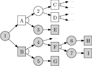
Figure 2: An and/or search tree used to illustrate our search mechanism. Circles are or nodes and represent problems, while boxes are and nodes and represent our rule applications. Nodes in grey are closed (solved).

We now describe the expansion of such a tree using an example. Consider the problem of removing a given element e from a list a. In our logical notation –using $\alpha$ as an abbreviation for $\mathsf{content}$– the problem is:

$$\left\llbracket a\mathop{,}e\ \left\langle\mathsf{true}\rhd\alpha(x)=\alpha(a)\setminus\{e\}\right\rangle\ x\right\rrbracket$$

We denote this problem by $1$ in the tree of Figure 2. While we haven’t given an exhaustive list of all rules used in our system, it is fair to assume that more than one can apply to this problem. For instance, we could case-split on the type of $a$, or apply List-rec to $a$. We represent these two options by A and B respectively in the tree.

Following the option B and applying List-rec with the path condition $\Pi_{2}\equiv\mathsf{true}$ trivially satisfies the first two premises of the rules, and generates two new problems ($5$ and $6$). Problem $5$ is:

$$\left\llbracket e\ \left\langle\mathsf{true}\rhd\alpha(x)=\alpha(\mathsf{Nil})\setminus\{e\}\right\rangle\ x\right\rrbracket$$

where the predicate simplifies to $\alpha(x)=\emptyset$. This makes it possible to apply the Ground rule (node G). This generates no subproblem, and closes the subbranch with the solution solution $\langle{\mathsf{true}}\mid{\mathsf{Nil}}\rangle$. Problem $4$ has the form:

$$\llbracket r\mathop{,}h\mathop{,}t\mathop{,}e\ \langle\alpha(r)=\alpha(t)\setminus\{e\}\rhd$$

$$\alpha(x)=\alpha(\mathsf{Cons(}h\mathsf{,}t\mathsf{)})\setminus\{e\}\rangle\ x\rrbracket$$

Among the many possible rule applications, we can choose to case-split on the equality $h=e$ (node F). This generates two subproblems. Problem $6$

$$\llbracket r\mathop{,}h\mathop{,}t\mathop{,}e\ \langle\alpha(r)=\alpha(t)\setminus\{e\}\land e=h\rhd$$

$$\alpha(x)=\alpha(\mathsf{Cons(}h\mathsf{,}t\mathsf{)})\setminus\{e\}\rangle\ x\rrbracket$$

and a similar problem $7$, where $e\neq h$ appears in the path condition instead of $e=h$. Both subproblems can be solved by using a technique we will describe in Section 6 to derive a term satisfying the synthesis predicate, effectively closing the complete branch from the root. The solutions for problem $6$ and $7$ are $\langle{\mathsf{true}}\mid{r}\rangle$ and $\langle{\mathsf{true}}\mid{\mathsf{Cons(}h\mathsf{,}r\mathsf{)}}\rangle$ respectively. A complete reconstruction of the solution given by the branch in gray yields the program:

⬇

def rec(a : List) : List = a match {

case Nil $\Rightarrow$ Nil

case Cons(h,t) $\Rightarrow$

val r = rec(t)

if(e == h) r

else Cons(h,r)

}

In the interest of space, we have only described the derivations that lead to the search. In practice of course, not all correct steps are taken in the right order. The interleaving of expansions of and and or nodes is driven by the estimated cost of problems and solutions.

Cost models.

In order to drive the search, we assign to each problem and to each rule application an estimated cost, which is supposed to under-approximate to actual final cost of a closed branch. For or nodes (problems), the cost is simply the minimum of all remaining viable children, while for and nodes (rule applications) we take the sum of the cost of each children plus a constant. That constant intuitively corresponds to the extra complexity inherent to a particular rule.

A perfect measure for cost would be the running time of the corresponding program. However, this is particularly hard to estimate, and valid under-approximations would most likely be useless. We chose to measure program size instead, as we expect it to be an reasonable proxy for complexity. We measure the size of the program as the number of branches, weighted by their proximity to the root. We found this to be have a positive influence on the quality of solutions, as it discourages near-top-level branching.

Using this metric, the cost inherent to a rule application roughly corresponds to the extra branches it introduces in the program. We use a standard algorithm for searching for the best solution Martelli and Montanari [1973], and the search thus always focuses on the current most promising solution. In our example in Figure 2, we could imagine that after the case split at F, the B branch temporarily became less attractive. The search then focuses for a while on the A branch, until expansion on that side (for instance by case-splitting on the type of the list) reached a point where the minimal possible solution was worse than the B branch. We note that the complete search takes about two seconds.

Anytime synthesis.

Because we maintain the search tree and know the current minimal solution at all times, we can stop the synthesis at any time and obtain a partial program that is likely to be good. This option is available in our implementation, both from the console mode and the web interface. In such cases, Leon will return a program containing new invocations of choose corresponding to the open subproblems.

6 Symbolic Term Exploration

In previous sections, we have introduced the notion of synthesis inference rules, and described how to search over rule applications that generate subproblems. In this section, we describe one of our most important rules, which is responsible for closing most of the branches in search trees. We call it Symbolic Term Exploration (STE).

The core idea behind STE is to symbolically represent many possible terms (programs), and to iteratively prune them out using counterexamples and test case generation until either 1) a valid term is proved to solve the synthesis problem or 2) all programs in the search spaces have been shown to be inadequate. Since we already have rules that take care of introducing branching constructs or recursive functions, we focus STE on the search for terms consisting only of constructors and calls to existing functions.

Recursive generators.

We start from a universal non-deterministic program that captures all the (deterministic) programs which we wish to consider as potential solutions. We then try to resolve the non-deterministic choices in such a way that the program realizes the desired property. Resolving the choices consists in fixing some values in the program, which we achieve by running a counterexample driven search.

We describe our non-deterministic programs as a set of recursive non-deterministic generators. Intuitively, a generator for a given type is a program that produces arbitrary values of that type. For instance, a generator for positive integers could be given by:

⬇

def genInt() : Int = if($\star$) 0 else (1 + genInt())

where $\star$ represents a non-deterministic boolean value. Similarly a non-deterministic generator for the List type could take the form:

⬇

def genList() : List = if($\star$) Nil else Cons(genInt(), genList())

It is not required that generators can produce every value for a given type; we could hypothesize for instance that our synthesis solutions will only need some very specific constants, such as $0$, $1$ or $-1$. What is more likely is that our synthesis solutions will need to use input variables and existing functions. Our generators therefore typically include variables of the proper type that are accessible in the synthesis environment. Taking these remarks into account, if a and b are integer variables in the scope, and f is a function from Int to Int, a typical generator for integers would be:

⬇

def genInt() : Int = if($\star$) 0 else if($\star$) 1 else if($\star$) -1

else if($\star$) a else if($\star$) b else f(genInt())

From generators to formulas.

Generators can in principle be any function with unresolved non-deterministic choices. For the sake of the presentation, we assume that they are “flat”, that is, they consist of a top-level non-deterministic choice between $n$ alternatives. (Note that the examples given above all have this form.)

Encoding a generator into an SMT term is straightforward: introduce for each invocation of a generator an uninterpreted constant $c$ of the proper type, and for each non-deterministic choice as many boolean variables $\bar{b}$ as there are alternatives. Encode that exactly one of the $\bar{b}$ variables must be true, and constrain the value of $c$ using the $\bar{b}$ variables.

Recursive invocations of generators can be handled similarly, by inserting another $c$ variable to represent their value and constraining it appropriately. Naturally, these recursive instantiations must stop at some point: we then speak of an instantiation depth. As an example, the encoding of the genList generator above with an instantiation depth of $1$ and assuming that genInt generates $0$ or $a$ is:

$$(b_{1}\lor b_{2})\land(\neg b_{1}\lor\neg b_{2})$$

$$\land~{}~{} b_{1}\Rightarrow c_{1}=\mathsf{Nil}\land b_{2}\Rightarrow c_{1}=\mathsf{Cons(}c_{2}\mathsf{,}c_{3}\mathsf{)}$$

$$\land~{}~{} (b_{3}\lor b_{4})\land(\neg b_{3}\lor\neg b_{4})$$

$$\land~{}~{} b_{3}\Rightarrow c_{2}=0\land b_{4}\Rightarrow c_{2}=a$$

$$\land~{}~{} (b_{5}\lor b_{6})\land(\neg b_{5}\lor\neg b_{6})$$

$$\land~{}~{} b_{5}\Rightarrow c_{3}=\mathsf{Nil}\land b_{6}\Rightarrow c_{3}=\mathsf{Cons(}c_{4}\mathsf{,}c_{5}\mathsf{)}$$

$$\land~{}~{} \neg b_{6}$$

The clauses encode the following possible values for $c_{1}$: Nil, Cons(0, Nil) and Cons(a, Nil). Note the constraint $\neg b_{6}$ which encodes the instantiation depth of $1$, by preventing the values beyond that depth (namely $c_{4}$ and $c_{5}$) to participate in the expression.

For a given instantiation depth, a valuation for the $\bar{b}$ variables encodes a determinization of the generators, and as a consequence a program. We solve for such a program by running a refinement loop.

Refinement loop: discovering programs.

Consider a synthesis problem $\left\llbracket\bar{a}\ \left\langle\Pi\rhd\phi\right\rangle\ \bar{x}\right\rrbracket$, where we speculate that a generator for the types of $\bar{x}$ can produce a program that realizes $\phi$. We start by encoding the non-deterministic execution of the generator for a fixed instantiation depth (typically, we start with $0$). Using this encoding, the problem has the form:

$$\phi\land B(\bar{a},\bar{b},\bar{c})\land C(\bar{c},\bar{x})$$ (2)

where $\phi$ is the synthesis problem, $B$ is the set of clauses obtained by encoding the execution of the generator and $C$ is a set of equalities tying $\bar{x}$ to a subset of the $\bar{c}$ variables. Note that by construction, the values for $\bar{c}$ (and therefore for $\bar{x}$) are uniquely determined when $\bar{a}$ and $\bar{b}$ are fixed.

We start by finding values for $\bar{a}$ and $\bar{b}$ such that (2) holds. If no such values exist, then our generators at the given instantiation depth are not expressive enough to encode a solution to the problem. Otherwise, we extract for the model the values $\bar{b}_{0}$. They describe a candidate program, which we put to the test.

Refinement loop: falsifying programs.

We search for a solution to the problem:

$$\neg\phi\land B(\bar{a},\bar{b}_{0},\bar{c})\land C(\bar{c},\bar{x})$$ (3)

Note that $\bar{b}_{0}$ are constants, and that $\bar{c}$ and $\bar{x}$ are therefore uniquely determined by $\bar{a}$ this intuitively comes from the fact that $\bar{b}_{0}$ encodes a deterministic program, that $\bar{c}$ encodes intermediate values in the execution of that program, and that $\bar{x}$ encodes the result. With this in mind, it becomes clear that we are really solving for $\bar{a}$.

If no such $\bar{a}$ exist, then we have found a program that realizes $\phi$ and we are done. If on the other hand we can find $\bar{a}_{0}$, then this constitutes an input that witnesses that our program does not meet the specification. In this case, we can discard the program by asserting $\neg\bigwedge\bar{b}$, and going back to (2).

Eventually, because the set of possible assignments to $\bar{b}$ is finite (for a given instantiation depth) this terminates. If we have not found a program, we can increase the instantiation depth and try again. When the maximal depth is reached, we give up.

Filtering with concrete execution.

While termination is in principle guaranteed just by successive elimination of programs in the refinement loop, the formula encoding the non-deterministic program typically grows exponentially as instantiation depth increases. As the number of programs grows, the difficulty for the solver to satisfy (2) or (3) also increases. As an alternative to symbolic elimination, we can often use concrete execution on a set of inputs to rule out many programs. We rely on Leon’s capability for small model finding (see Section 3) to generate inputs that satisfy the path condition. We then use on-the-fly code generation to compile the symbolic program into a function that takes as arguments the input variables as well as a boolean array encoding the non-deterministic choices. This allows us to rapidly discard hundreds or even thousand of programs. Whenever the change is substantial, we regenerate a new formula for (2) with much fewer boolean variables and continue from there. Note that very often, when STE is applied to a problem it cannot solve, concrete execution rules out all programs in a fraction of a second and symbolic reasoning is never applied.

7 Type-Driven Counterexample-Guided Synthesis with Condition Abduction

Our second larger rule focuses on synthesizing recursive functions that satisfy a given specification. We assume that we are given a function header and a postcondition, and that we aim to synthesize a recursive function body. Note that the expression must be 1) a well-typed term with respect to the context of the program and 2) valid according to the imposed formal specification. Therefore, an approach to solve this kind of synthesis problems could be based on searching the space of all expressions that can be built from all declarations visible at the corresponding place in the program, i.e. in the scope of choose, while limiting attention to those that type-check, have the desired type, and satisfy the given formal specification.

An obvious drawback of such approach is that, unless the process is carefully guided, the search becomes unfeasible due to search space explosion. In practice we indeed found that trivial generate-and-test strategies scale poorly with the number of visible declarations and the search becomes practically unfeasible even for small programs.

7.1 Condition Abduction

Our idea for guiding the search and incremental construction of correct expressions comes from the area of abductive reasoning Josephson [1994]; Kakas et al. [1992]. Abductive reasoning, sometimes also called “inference to the best explanation”, is a method of reasoning in which one chooses a hypothesis that would explain the observed evidence in the best way.

The motivation behind the approach to applying abductive reasoning to program synthesis comes from examining implementations of practical purely functional, recursive algorithms. The key observation is that recursive functional algorithms share a similar pattern. They implement behaviour through a combination of case analysis with control flow expressions (e.g. if-then-else) and recursive calls. This pattern is encoded with a branching control flow expression that partitions the space of input values such that each branch represents a correct implementation for a certain partition. Such partitions are defined by conditions that guard branches in the control flow.

This allows synthesizing branches separately by searching for implementations that evaluate correctly only for certain inputs while restricting the search space. Rather than speculatively applying Case-split rule to obtain subproblems and finding solutions for each branch by case analysis (as described in Section 4), this idea applies a similar strategy in the reverse order – getting a candidate program and searching for a condition that would make it correct. Thus, the idea of abductive reasoning can be applied to guess the condition that defines a valid partition, i.e. “abduce” the explanation for a partial implementation, with respect to a given candidate program. The rule progressively applies this technique and enables effective search and construction of a control flow expression that represents a correct implementation for more and more input cases, eventually constructing an expression that is a solution to the synthesis problem.

7.2 The Algorithm Used in the Rule

Based on these observations, we present our rule that employs a new technique for guiding the search with ranking and filtering based on counterexamples, as well as constructing expressions from partially correct implementations. It is presented in Algorithm 1.

Algorithm 1 Synthesis with condition abduction

1:path condition $\Pi$, predicate $\phi$, a collection of    expressions $s$ $\triangleright$ synthesis problem $\left\llbracket\bar{a}\ \left\langle\Pi\rhd\phi\right\rangle\ \bar{x}\right\rrbracket$

2:$p^{\prime}=true$ $\triangleright$ maintain the current partition

3:$sol=(\lambda x.x)$ $\triangleright$ maintain a partial solution

4:$\mathcal{M}=$ SampleModels($\bar{a}$) $\triangleright$ set of example models

5:repeat

6:   get a set of expressions $E$ from $s$ $\triangleright$ candidates

7:   for each $e$ in $E$ do $\triangleright$ count passed examples $p_{e}$ for $e$

8:     $p_{e}=|\{m\in\mathcal{M}\mid e(m)\mbox{ is correct}\}|$ $\triangleright$ evaluate    

9:   $\bar{r}=\arg\max_{\;e\in E\;}p_{e}$ $\triangleright$ the highest ranked expression

10:   if solution $\langle{\Pi\wedge p^{\prime}}\mid{\bar{r}}\rangle$ is valid then

11:     return $\langle{\Pi}\mid{(sol\;\bar{r})}\rangle$ $\triangleright$ a solution is found

12:   else

13:     extract new counterexample model $m$

14:     $\mathcal{M}=\mathcal{M}\cup m$ $\triangleright$ accumulate examples

15:     $c=$ BranchSyn($\bar{r},p,q,s$) $\triangleright$ call Algorithm 2

16:     if $c\neq$ false then $\triangleright$ a branch is synthesized

17:        $sol=(\lambda x.$ $(sol\;($if $c$ then $\bar{r}$ else $x)))$

18:        $p^{\prime}=p^{\prime}\wedge\neg c$ $\triangleright$ update current partition         

19:until $s$ is not empty

The algorithm applies the idea of abducing conditions to progressively synthesize and verify branches of a correct implementation for an expanding partition of inputs. The input to the algorithm is a path condition $\Pi$, a predicate $\phi$ (defined by synthesis problem $\left\llbracket\bar{a}\ \left\langle\Pi\rhd\phi\right\rangle\ \bar{x}\right\rrbracket$), and a collection of expressions $s$.

Condition $p^{\prime}$ defines which inputs are left to consider at any given point in the algorithm; these are the inputs that belong to the current partition. The initial value of $p^{\prime}$ is $true$, so the algorithm starts with a partition that covers the whole initial input space constrained only by the path condition $\Pi$. Let $p_{1},\ldots,p_{k}$, where $k>0$, be conditions abduced up to a certain point in the algorithm. Then $p^{\prime}$ represents the conjunction of negations of abduced conditions, i.e. $p^{\prime}=\neg p_{1}\wedge\ldots\wedge\neg p_{k}$. Together with the path condition, it defines the current partition which includes all input values for which there is no condition abduced (nor correct implementation found). Thus, the guard condition for the current partition is defined by $\Pi\wedge p^{\prime}$. The algorithm maintains the partial solution $sol$, encoded as a function. $sol$ encodes an expression which is correct for all input values that satisfy any of the abduced conditions and this expression can be returned as a partial solution at any point. Additionally, the algorithm accumulates example models in the set $\mathcal{M}$. Ground term generator, described in Section 3, is used to construct the initial set of models in $\mathcal{M}$. To construct a model, for each variable in $\bar{a}$, the algorithm assigns a value sampled from the ground term generator. Note that more detailed discussion on how examples are used to guide the search is deferred to Section 7.3.

The algorithm repeats enumerating all possible expressions from the given collection until it finds a solution. In each iteration, a batch of expressions $E$ is enumerated and evaluated on all models from $\mathcal{M}$. The results of such evaluation are used to rank expressions from $E$. The algorithm considers the expression of the highest rank $\bar{r}$ as a candidate solution and checks it for validity. If $\bar{r}$ represents a correct implementation for the current partition, i.e. if $\langle{\Pi\wedge p^{\prime}}\mid{\bar{r}}\rangle$ is a valid solution, then the expression needed to complete a valid control flow expression is found. The algorithm returns it as solution for which $\left\llbracket\bar{a}\ \left\langle\Pi\rhd\phi\right\rangle\ \bar{x}\right\rrbracket\vdash\langle{\Pi}\mid{(sol\;\bar{r})}\rangle$ holds. Otherwise, the algorithm extracts the counterexample model $m$, adds it to the set $\mathcal{M}$, and continues by trying to synthesize a branch with expression $\bar{r}$ (it does so by calling Algorithm 2 which will be explained later). If BranchSyn returns a valid branch condition, the algorithm updates the partial solution to include the additional branch (thus extending extending the space of inputs covered by the partial solution), and refines the current partition condition. New partition condition reduces the synthesis to a subproblem, ensuring that the solution in the next iteration covers cases where $c$ does not hold. The algorithm eventually, given the appropriate terms from $s$, finds an expression that forms a complete correct implementation for the synthesis problem.

Algorithm 2 Synthesize a branch

1:expression $\bar{r}$, condition $p^{\prime}$, predicate $q$, and a    collection of expressions $s$ $\triangleright$ passed from Algorithm 1

2:function BranchSyn($\bar{r},p^{\prime},q,s$)

3:   $\mathcal{M^{\prime}}=\emptyset$ $\triangleright$ set of accumulated counterexamples

4:   get a set of expressions $E^{\prime}$ from $s$ $\triangleright$ candidates

5:   for each $c$ in $E^{\prime}$ do

6:     if for each model $m$ in $\mathcal{M^{\prime}}$, $c(m)=false$ then

7:        if  solution $\langle{\Pi\wedge c}\mid{\bar{r}}\rangle$ is valid  then

8:          return $c$ $\triangleright$ a condition is abduced

9:        else

10:          extract the new counterexample model $m$

11:          $\mathcal{M^{\prime}}=\mathcal{M^{\prime}}\cup m$ $\triangleright$ accumulate counterexamples                 

12:   return false $\triangleright$ no condition is found

Algorithm 2 tries to synthesize a new branch by abducing a valid branch condition $c$. It does this by enumerating a set of expressions $E^{\prime}$ from $s$ and checking whether it can find a valid condition expression, that would guard a partition for which the candidate expression $\bar{r}$ is correct.The algorithm accumulates counterexamples models in $\mathcal{M^{\prime}}$ and considers a candidate expression $c$ only if it prevents all accumulated counterexamples.The algorithm checks this by evaluating $c$ on $m$, i.e. $c(m)$, for each accumulated counterexample $m$. If a candidate expression $c$ is not filtered out, the algorithm checks if $c$ represents a valid branch condition, i.e. whether $\langle{\Pi\wedge c}\mid{\bar{r}}\rangle$ is a valid solution. If yes, the algorithm returns $c$ which, together with $\bar{r}$, comprises a valid branch in the solution to $\left\llbracket\bar{a}\ \left\langle\Pi\rhd\phi\right\rangle\ \bar{x}\right\rrbracket$. Otherwise, it adds a new counterexample model to $\mathcal{M^{\prime}}$ and continues with the search. If no valid condition is in $E^{\prime}$, the algorithm returns false.

7.3 Organization of the Search

For getting the collection of expressions $s$, the rule uses term generators that generate all well typed terms according to type constraints derived from the context of a program Gvero et al. [2013]; Kuraj [2013]. This has the advantage of initial search space restriction inherent to the generator that limits enumerated expressions only to those that are well typed. The completeness property of such generators ensures systematic enumeration of all candidate solutions that are defined by the set of given type constraints. For verification, the rule uses the Leon verifier, that allows checking validity of expressions that are supported by the underlying theories and obtaining counterexample models.

The context of the algorithm as a rule in the Leon synthesis framework imposes limits on the portion of search space explored by each rule instantiation. This allows incremental and systematic progress in search space exploration and, due to the mixture with other synthesis rules, offers benefits in both expressiveness and performance of synthesis. The rule offers flexibility in adjusting necessary parameters and thus a fine-grain control over the search - for our experiments, the size of candidate sets of expressions enumerated in each iteration $n$ is 50 (and is doubled in each iteration) and 20, in the case of Algorithm 1 and 2, respectively.

Using (counter-)examples.

A technique that brings significant performance improvements when dealing with large search spaces is guiding the search and even avoid considering candidate expressions according to the information from examples generated during synthesis. As described earlier, after checking an unsatisfiable formula, the rule queries Leon for the witness model and accumulates examples that are used to narrow down the search space.

Algorithm 2 uses accumulated counterexamples to filter out unnecessary candidate expressions when synthesizing a branch. It makes sense to consider a candidate expression for a branch condition, $c$, for a check whether $c$ makes $\bar{r}$ a correct implementation, only if $c$ prevents all accumulated counterexamples that already witnessed unsatisfiability of the correctness formula for $\bar{r}$, i.e. if $\forall m\in\mathcal{M^{\prime}}.\;c\rightarrow\neg m$. Otherwise, if $\exists m\in\mathcal{M^{\prime}}.\neg(c\rightarrow\neg m)$, then $m$ is a valid counterexample to the verification of $\langle{\Pi\wedge c}\mid{\bar{r}}\rangle$. This effectively guides the search by the results of previous verification failures while filtering out candidates before more expensive verification check are made.

Algorithm 1 uses accumulated models to quickly test and rank expressions by evaluating models according to the specification. The current set of candidate expressions $E$ is evaluated on the set of accumulated examples $\mathcal{M}$ and results of such evaluation are used to rank the candidates. We call an evaluation of a candidate $e$ on a model $m$ correct, if $m$ satisfies path condition $\Pi$ and the result of the evaluation satisfies given predicate $q$. The algorithm counts the number of correct evaluations, ranks the candidates accordingly and considers only the candidate of the highest rank. The rationale is that the more correct evaluations, the more likely the candidate represents a correct implementation for some partition of inputs. Note that evaluation results may be used only for ranking but not for filtering, because each candidate may represent a correct implementation for a certain partition of inputs, thus incorrect evaluations are expected even for valid candidates. Since the evaluation amounts to executing the specification this technique is efficient in guiding the search toward correct correct implementations while avoiding unnecessary verification checks.

Operation	Syn	Size	Calls	sec.	Proved
List.Insert	$\surd$	3	0	0.3	$\surd$
List.Delete	$\surd$	19	1	2.0	$\surd$
List.Union	$\surd$	12	1	2.0	$\surd$
List.Diff	$\surd$	12	2	7.0	$\surd$
List.Split	$\surd$	27	1	2.0	$\surd$
SortedList.Insert	$\surd$	34	1	8.9	$\surd$
SortedList.InsertAlways	$\surd$	36	1	12.5	$\surd$
SortedList.Delete	$\surd$	23	1	8.7
SortedList.Union	$\surd$	19	2	5.0	$\surd$
SortedList.Diff	$\surd$	13	2	6.8
SortedList.InsertionSort	$\surd$	10	2	5.1	$\surd$
SortedList.MergeSort	$\surd$	11	4	87.7	$\surd$
StrictSortedList.Insert	$\surd$	34	1	9.9	$\surd$
StrictSortedList.Delete	$\surd$	21	1	16.1
StrictSortedList.Union	$\surd$	19	2	4.1	$\surd$
UnaryNumerals.Add	$\surd$	11	1	1.6	$\surd$
UnaryNumerals.Distinct	$\surd$	12	0	1.9	$\surd$
UnaryNumerals.Mult	$\surd$	12	1	2.5	$\surd$

Figure 3: We consider a problem as synthesized if the solution generated is correct after manual inspection. For each generated program, we provide the size of its syntax tree and the number of function calls it contains. Proved problems are those for which the synthesized program can be automatically proven to match its specification.

8 Implementation and Results

We have implemented these techniques in Leon, a system for verification and synthesis of functional program, thus extending it from the state described in Section 3. Our implementation and the online interface are available from http://lara.epfl.ch/leon/.

The front end to Leon is the standard Scala compiler (for Scala 2.9). Scala compiler performs type checking and tasks such as the expansion of implicit conversions, from which Leon directly benefits. Leon programs also execute as valid Scala programs. Leon checks that the syntax trees produced conform to the subset that it expects and then performs verification and synthesis.

We have developed several interfaces for Leon. Leon can be invoked as a batch command-line tool that accepts verification and synthesis tasks and outputs the results of the requested tasks. If desired, there is also a console mode that allows applying synthesis rules in a step-by-step fashion and is useful for debugging purposes.

To facilitate interactive experiments and the use of the system in teaching, we have also developed an interface that executes in the web browser, using the Play framework of Scala as well as JavaScript editors. Our browser-based interface supports continuous compilation of Scala code, allows verifying individual functions with a single keystroke or click, as well as synthesizing any given choose expression. In cases when the synthesis process is interrupted, the synthesizer can generate a partial solution that contains a program with further occurrences of the choose statement.

8.1 Results

In order to evaluate our system, we developed benchmarks with reusable abstraction functions. These abstraction functions allow for a concise specification of each operation without requiring any insight on its resulting implementation. It is interesting to notice that these functions generally abstract any structural invariant inherent to the underlying data-structure. For instance, the synthesis of

⬇

def add(a: Num, b: Num) = choose {

(res: Num) $\Rightarrow$ value(r) == value(a) + value(b)

}

would result in vastly different programs depending on the implementation of Number.

Our set of benchmarks displayed in Figure 3 covers the synthesis of various operations over custom data-structures with invariants, specified through the lens of abstraction functions. These benchmarks use specifications with are both easy to understand and much shorter than resulting programs (except in trivial cases). We believe these are key factors in the evaluation of any synthesis procedure. The definitions and specifications of all the benchmarks can be found in appendix.

Synthesis is performed in order, meaning that an operation will be able to reuse all previously synthesized ones, thus mimicking the usual development process.

We can see in Figure 3 the list of programs we successfully synthesized. Each synthesized program has been manually validated to be a solution that a programmer might expect. Our system typically also proves automatically that the resulting program matches the specification for all inputs. In certain cases, the lack of inductive invariants prevents such fully-automated proof, which is a limitation of our verifier. Note that we stop verification after a timeout of 3 seconds.

In almost all cases, the synthesis succeeds sufficiently fast for a reasonable interactive experience.

9 Related Work

Our approach blends deductive synthesis Manna and Waldinger [1971, 1980]; Smith [2005], which incorporates transformation of specifications, inductive reasoning, recursion schemes and termination checking, with modern SMT techniques and constraint solving for executable constraints. As one of our subroutines we include complete functional synthesis for integer linear arithmetic Kuncak et al. [2012] and extend it with complete functional synthesis for algebraic data types Suter [2012]; Jacobs et al. [2013]. This gives us building blocks for synthesis of recursion-free code. To synthesize recursive code we build on and further advance the counterexample-guided approach to synthesis Solar-Lezama et al. [2006].

Deductive synthesis frameworks.

Early work on synthesis Manna and Waldinger [1971, 1980] focused on synthesis using expressive and undecidable logics, such as first-order logic and logic containing the induction principle.

Programming by refinement has been popularized as a manual activity Wirth [1983]; Back and von Wright [1998]. Interactive tools have been developed to support such techniques in HOL Butler et al. [1997]. A recent example of deductive synthesis and refinement is the Specware system from Kesterel Smith [2005]. We were not able to use the system first-hand due to its availability policy, but it appears to favor expressive power and control, whereas we favor automation.

A combination of automated and interactive development is analogous to the use of automation in interactive theorem provers, such as Isabelle Nipkow et al. [2002]. However, whereas in verification it is typically the case that the program is available, the emphasis here is on constructing the program itself, starting from specifications.

Work on synthesis from specifications Srivastava et al. [2010] resolves some of these difficulties by decoupling the problem of inferring program control structure and the problem of synthesizing the computation along the control edges. The work leverages verification techniques that use both approximation and lattice theoretic search along with decision procedures, but appears to require more detailed information about the structure of the expected solution than our approach.

Synthesis with input/output examples.

One of the first works that addressed synthesis with examples and put inductive synthesis on a firm theoretical foundation is the one by Summers Summers [1977]. Subsequent work presents extensions of the classical approach to induction of functional Lisp-programs Kitzelmann and Schmid [2006]; Hofmann [2010]. These extensions include synthesizing a set of equations (instead of just one), multiple recursive calls and systematic introduction of parameters. Our current system lifts several restrictions of previous approaches by supproting reasoning about arbitrary datatypes, supporting multiple parameters in concrete and symbolic I/O examples, and allowing nested recursive calls and user-defined declarations.

Inductive (logic) programming that explores automatic synthesis of (usually recursive) programs from incomplete specifications, most often being input/output examples Flener and Partridge [2001]; Muggleton and Raedt [1994], influenced our work. Recent work in the area of programming by demonstration has shown that synthesis from examples can be effective in a variety of domains, such as spreadsheets Singh and Gulwani [2012]. Advances in the field of SAT and SMT solvers inspired counter-example guided iterative synthesis Solar-Lezama et al. [2006]; Gulwani et al. [2011], which can derive input and output examples from specifications. Our tool uses and advances these techniques through two new counterexample-guided synthesis approaches.

Synthesis based on finitization techniques.

Program sketching has demonstrated the practicality of program synthesis by focusing its use on particular domains Solar-Lezama et al. [2006, 2007, 2008]. The algorithms employed in sketching are typically focused on appropriately guided search over the syntax tree of the synthesized program. The tool we presented shows one way to move the ideas of sketching towards infinite domains. In this generalization we leverage reasoning about equations as much as SAT techniques.

Reactive synthesis.

Synthesis of reactive systems generates programs that run forever and interact with the environment. However, known complete algorithms for reactive synthesis work with finite-state systems Pnueli and Rosner [1989] or timed systems Asarin et al. [1995]. Such techniques have applications to control the behavior of hardware and embedded systems or concurrent programs Vechev et al. [2009]. These techniques usually take specifications in a fragment of temporal logic Piterman et al. [2006] and have resulted in tools that can synthesize useful hardware components Jobstmann et al. [2007]; Jobstmann and Bloem [2006]. Recently such synthesis techniques have been extended to repair that preserves good behaviors Essen and Jobstmann [2013], which is related to our notion of partial programs that have remaining choose statements.

10 Conclusions and Analysis

Software synthesis is a difficult problem but we believe it can provide substantial help in software development. We have presented a new framework for synthesis that combines transformational and counterexample-guided approaches. Our implemented system can synthesize and prove correct functional programs that manipulate unbounded data structures such as algebraic data types. We have used the system to synthesized algorithms that manipulate list and tree structures. The algorithm can be combined with manual transformations or run-time constraint solving to cover the cases where static synthesis does not fully solve the problem. Our current counterexample-guided synthesis steps are domain-agnostic, while somewhat limits their scalability, so we expect improved results using domain-specific generators, such as the ones used in testing tools UDITA Gligoric et al. [2010] and Quickcheck Claessen and Hughes [2000]. Our framework leverages the state of the art SMT solving technology and an effective mechanism for solving certain classes of recursive functions. Thanks to this technology, it was able to synthesize programs over unbounded domains that are guaranteed to be correct for all inputs.

We thank Regis Blanc for his contribution to the Leon verification infrastructure. We thank Tihomir Gvero and Ruzica Piskac for many discussions on synthesis.

Appendix A Benchmarks Definitions

A.1 List

⬇

object ListBenchmark {

sealed abstract class List

case class Cons(head: Int, tail: List) extends List

case object Nil extends List

def size(l: List) : Int = (l match {

case Nil $\Rightarrow$ 0

case Cons(_, t) $\Rightarrow$ 1 + size(t)

}) ensuring(res $\Rightarrow$ res $\geq$ 0)

def content(l: List): Set[Int] = l match {

case Nil $\Rightarrow$ Set.empty[Int]

case Cons(i, t) $\Rightarrow$ Set(i) ++ content(t)

}

def abs(i : Int) : Int = {

if(i < 0) -i else i

} ensuring(_ $\geq$ 0)

def insert(in1: List, v: Int) = choose {

(out : List) $\Rightarrow$

content(out) == content(in1) ++ Set(v)

}

def delete(in1: List, v: Int) = choose {

(out : List) $\Rightarrow$

content(out) == content(in1) -- Set(v)

}

def union(in1: List, in2: List) = choose {

(out : List) $\Rightarrow$

content(out) == content(in1) ++ content(in2)

}

def diff(in1: List, in2: List) = choose {

(out : List) $\Rightarrow$

content(out) == content(in1) -- content(in2)

}

def split(list : List) : (List,List) = {

choose { (res : (List,List)) $\Rightarrow$

val s1 = size(res._1)

val s2 = size(res._2)

abs(s1 - s2) $\leq$ 1 && s1 + s2 == size(list) &&

content(res._1) ++ content(res._2) == content(list)

}

}

}

A.2 SortedList

⬇

object SortedListBenchmark {

sealed abstract class List

case class Cons(head: Int, tail: List) extends List

case object Nil extends List

def size(l: List) : Int = (l match {

case Nil $\Rightarrow$ 0

case Cons(_, t) $\Rightarrow$ 1 + size(t)

}) ensuring(res $\Rightarrow$ res $\geq$ 0)

def content(l: List): Set[Int] = l match {

case Nil $\Rightarrow$ Set.empty[Int]

case Cons(i, t) $\Rightarrow$ Set(i) ++ content(t)

}

def isSorted(list : List) : Boolean = list match {

case Nil $\Rightarrow$ true

case Cons(_, Nil) $\Rightarrow$ true

case Cons(x1, Cons(x2, _)) if(x1 > x2) $\Rightarrow$ false

case Cons(_, xs) $\Rightarrow$ isSorted(xs)

}

def insert(in1: List, v: Int) = choose {

(out : List) $\Rightarrow$

isSorted(in1) &&

(content(out) == content(in1) ++ Set(v)) &&

isSorted(out)

}

def insertAlways(in1: List, v: Int) = choose {

(out : List) $\Rightarrow$

isSorted(in1) &&

(content(out) == content(in1) ++ Set(v)) &&

isSorted(out) &&

size(out) == size(in1) + 1

}

def delete(in1: List, v: Int) = choose {

(out : List) $\Rightarrow$

isSorted(in1) &&

(content(out) == content(in1) -- Set(v)) &&

isSorted(out)

}

def union(in1: List, in2: List) = choose {

(out : List) $\Rightarrow$

isSorted(in1) &&

isSorted(in2) &&

(content(out) == content(in1) ++ content(in2)) &&

isSorted(out)

}

def diff(in1: List, in2: List) = choose {

(out : List) $\Rightarrow$

isSorted(in1) &&

isSorted(in2) &&

(content(out) == content(in1) -- content(in2)) &&

isSorted(out)

}

// In order to synthesize insertionSort, we let

// insert in the scope. Similarly for mergeSort,

// we keep only split and union in the scope.

def sort(list: List): List = choose {

(res: List) $\Rightarrow$

isSorted(res) &&

content(res) == content(list)

}

}

A.3 StrictlySortedList

⬇

object Complete {

sealed abstract class List

case class Cons(head: Int, tail: List) extends List

case object Nil extends List

def size(l: List) : Int = (l match {

case Nil $\Rightarrow$ 0

case Cons(_, t) $\Rightarrow$ 1 + size(t)

}) ensuring(res $\Rightarrow$ res $\geq$ 0)

def content(l: List): Set[Int] = l match {

case Nil $\Rightarrow$ Set.empty[Int]

case Cons(i, t) $\Rightarrow$ Set(i) ++ content(t)

}

def isSorted(list : List) : Boolean = list match {

case Nil $\Rightarrow$ true

case Cons(_, Nil) $\Rightarrow$ true

case Cons(x1, Cons(x2, _)) if(x1 $\geq$ x2) $\Rightarrow$ false

case Cons(_, xs) $\Rightarrow$ isSorted(xs)

}

def insert(in1: List, v: Int) = choose {

(out : List) $\Rightarrow$

isSorted(in1) &&

(content(out) == content(in1) ++ Set(v)) &&

isSorted(out)

}

def delete(in1: List, v: Int) = choose {

(out : List) $\Rightarrow$

isSorted(in1) &&

(content(out) == content(in1) -- Set(v)) &&

isSorted(out)

}

def union(in1: List, in2: List) = choose {

(out : List) $\Rightarrow$

isSorted(in1) &&

isSorted(in2) &&

(content(out) == content(in1) ++ content(in2)) &&

isSorted(out)

}

}

A.4 UnaryNumerals

⬇

object UnaryNumeralsBenchmark {

sealed abstract class Num

case object Z extends Num

case class S(pred: Num) extends Num

def value(n:Num) : Int = {

n match {

case Z $\Rightarrow$ 0

case S(p) $\Rightarrow$ 1 + value(p)

}

} ensuring (_ $\geq$ 0)

def add(x: Num, y: Num): Num = {

choose { (r : Num) $\Rightarrow$

value(r) == value(x) + value(y)

}

}

def distinct(x: Num, y: Num): Num = {

choose { (r : Num) $\Rightarrow$

value(r) != value(x) &&

value(r) != value(y)

}

}

def mult(x: Num, y: Num): Num = {

choose { (r : Num) $\Rightarrow$

value(r) == value(x) * value(y)

}

}

}

References

- Asarin et al. [1995] E. Asarin, O. Maler, and A. Pnueli. Symbolic controller synthesis for discrete and timed systems. In Hybrid Systems II, pages 1–20, 1995.
- Back and von Wright [1998] R.-J. Back and J. von Wright. Refinement Calculus. Springer-Verlag, 1998.
- Barnett et al. [2011] M. Barnett, M. Fähndrich, K. R. M. Leino, P. Müller, W. Schulte, and H. Venter. Specification and verification: the Spec# experience. Commun. ACM, 54(6), June 2011.
- Butler et al. [1997] M. Butler, J. Grundy, T. Langbacka, R. Ruksenas, and J. von Wright. The refinement calculator: Proof support for program refinement. In Proc. Formal Methods Pacific ’97, 1997.
- Claessen and Hughes [2000] K. Claessen and J. Hughes. Quickcheck: a lightweight tool for random testing of haskell programs. In ICFP, pages 268–279, 2000.
- Essen and Jobstmann [2013] C. V. Essen and B. Jobstmann. Program repair without regret. In CAV, 2013.
- Flener and Partridge [2001] P. Flener and D. Partridge. Inductive programming. Autom. Softw. Eng., 8(2):131–137, 2001.
- Gligoric et al. [2010] M. Gligoric, T. Gvero, V. Jagannath, S. Khurshid, V. Kuncak, and D. Marinov. Test generation through programming in UDITA. In ICSE, pages 225–234, 2010.
- Gulwani et al. [2011] S. Gulwani, S. Jha, A. Tiwari, and R. Venkatesan. Synthesis of loop-free programs. In PLDI, pages 62–73, 2011.
- Gvero et al. [2013] T. Gvero, V. Kuncak, I. Kuraj, and R. Piskac. Complete completion using types and weights. In PLDI, 2013.
- Hofmann [2010] M. Hofmann. IgorII - an analytical inductive functional programming system (tool demo). In PEPM, pages 29–32, 2010.
- Jacobs et al. [2013] S. Jacobs, V. Kuncak, and P. Suter. Reductions for synthesis procedures. In VMCAI, pages 88–107, 2013.
- Jaffar and Lassez [1987] J. Jaffar and J.-L. Lassez. Constraint logic programming. In POPL, 1987.
- Jobstmann and Bloem [2006] B. Jobstmann and R. Bloem. Optimizations for LTL synthesis. In FMCAD, 2006.
- Jobstmann et al. [2007] B. Jobstmann, S. Galler, M. Weiglhofer, and R. Bloem. Anzu: A tool for property synthesis. In CAV, 2007.
- Josephson [1994] J. R. Josephson. Abductive Inference: Computation, Philosophy, Technology. Cambridge University Press, 1994.
- Kakas et al. [1992] A. C. Kakas, R. A. Kowalski, and F. Toni. Abductive logic programming. J. Log. Comput., 2(6):719–770, 1992.
- Kitzelmann and Schmid [2006] E. Kitzelmann and U. Schmid. Inductive synthesis of functional programs: An explanation based generalization approach. JMLR, 7:429–454, 2006.
- Klein et al. [2009] G. Klein, J. Andronick, K. Elphinstone, G. Heiser, D. Cock, P. Derrin, D. Elkaduwe, K. Engelhardt, R. Kolanski, M. Norrish, T. Sewell, H. Tuch, and S. Winwood. seL4: Formal verification of an OS kernel. In SOSP, pages 207–220, 2009.
- Köksal et al. [2012] A. S. Köksal, V. Kuncak, and P. Suter. Constraints as control. In POPL, pages 151–164, 2012.
- Kuncak et al. [2010] V. Kuncak, M. Mayer, R. Piskac, and P. Suter. Complete functional synthesis. In PLDI, pages 316–329, 2010.
- Kuncak et al. [2012] V. Kuncak, M. Mayer, R. Piskac, and P. Suter. Software synthesis procedures. CACM, 55(2):103–111, 2012.
- Kuraj [2013] I. Kuraj. Interactive code generation. Master’s thesis, EPFL, February 2013.
- Leinenbach and Santen [2009] D. Leinenbach and T. Santen. Verifying the microsoft hyper-v hypervisor with VCC. In FM, 2009.
- Manna and Waldinger [1971] Z. Manna and R. J. Waldinger. Toward automatic program synthesis. Commun. ACM, 14(3):151–165, 1971.
- Manna and Waldinger [1980] Z. Manna and R. J. Waldinger. A deductive approach to program synthesis. ACM Trans. Program. Lang. Syst., 2(1):90–121, 1980.
- Martelli and Montanari [1973] A. Martelli and U. Montanari. Additive AND/OR graphs. In IJCAI, pages 1–11, 1973.
- McCarthy [1960] J. McCarthy. Recursive functions of symbolic expressions and their computation by machine, part 1. Comm. A.C.M., 3:184–195, 1960.
- de Moura and Bjørner [2008] L. de Moura and N. Bjørner. Z3: An efficient SMT solver. In TACAS, 2008.
- Muggleton and Raedt [1994] S. Muggleton and L. D. Raedt. Inductive logic programming: Theory and methods. J. Log. Program., 19/20:629–679, 1994.
- Nipkow et al. [2002] T. Nipkow, L. C. Paulson, and M. Wenzel. Isabelle/HOL: A Proof Assistant for Higher-Order Logic, volume 2283 of LNCS. Springer-Verlag, 2002.
- Odersky [2010] M. Odersky. Contracts for scala. In RV, pages 51–57, 2010.
- Piterman et al. [2006] N. Piterman, A. Pnueli, and Y. Sa’ar. Synthesis of reactive(1) designs. In VMCAI, 2006.
- Pnueli and Rosner [1989] A. Pnueli and R. Rosner. On the synthesis of a reactive module. In POPL, 1989.
- Singh and Gulwani [2012] R. Singh and S. Gulwani. Synthesizing number transformations from input-output examples. In CAV, pages 634–651, 2012.
- Smith [2005] D. R. Smith. Generating programs plus proofs by refinement. In VSTTE, 2005.
- Solar-Lezama et al. [2006] A. Solar-Lezama, L. Tancau, R. Bodík, S. A. Seshia, and V. A. Saraswat. Combinatorial sketching for finite programs. In ASPLOS, 2006.
- Solar-Lezama et al. [2007] A. Solar-Lezama, G. Arnold, L. Tancau, R. Bodík, V. A. Saraswat, and S. A. Seshia. Sketching stencils. In PLDI, pages 167–178, 2007.
- Solar-Lezama et al. [2008] A. Solar-Lezama, C. G. Jones, and R. Bodík. Sketching concurrent data structures. In PLDI, 2008.
- Srivastava et al. [2010] S. Srivastava, S. Gulwani, and J. S. Foster. From program verification to program synthesis. In POPL, 2010.
- Summers [1977] P. D. Summers. A methodology for LISP program construction from examples. JACM, 24(1):161–175, 1977.
- Suter [2012] P. Suter. Programming with Specifications. PhD thesis, EPFL, December 2012.
- Suter et al. [2010] P. Suter, M. Dotta, and V. Kuncak. Decision procedures for algebraic data types with abstractions. In POPL, pages 199–210, 2010.
- Suter et al. [2011] P. Suter, A. S. Köksal, and V. Kuncak. Satisfiability modulo recursive programs. In SAS, pages 298–315, 2011.
- Vechev et al. [2009] M. T. Vechev, E. Yahav, and G. Yorsh. Inferring synchronization under limited observability. In TACAS, 2009.
- Wirth [1983] N. Wirth. Program development by stepwise refinement (reprint). Commun. ACM, 26(1):70–74, 1983.