High precision measurement of ultraweak transitions of the a${{}^{1}}{\triangle}_{g}{\leftarrow}$X ${}^{3}{\Sigma}^{-}_{g}$ $(0,0)$ band of molecular oxygen

Abstract

We have used a highly sensitive cavity-enhanced frequency modulation spectroscopy technique to measure different parameters of the ultraweak transitions of a${{}^{1}}{\triangle}_{g}{\leftarrow}$X ${}^{3}{\Sigma}^{-}_{g}$ $(0,0)$ band of molecular oxygen in the range 7640 cm^-1 to 7917 cm^-1. The self-broadened half-width and air-broadened half-width of the transitions have been measured for three different pressures for both ¹⁶O₂ and ¹⁸O₂. To measure the line intensity and self-broadened half-width we have used ultra pure oxygen sample and air-broadened half-width was measured with dry air sample. The $(0,0)$ band of ¹⁶O₂ and ¹⁸O₂ show weak quadrupole transitions with line intensities ranging from $1\times 10^{-30}$ to $1.9\times 10^{-28}$ cm/molecule. The measurements are in excellent agreement with the recent measurement of Rothman et. al. [1].

1 Introduction

The precise measurement of different parameters in the infrared spectrum in the a${{}^{1}}{\triangle}_{g}{\leftarrow}$X ${}^{3}{\Sigma}^{-}_{g}$ $(0,0)$ band of oxygen is of fundamental interest to the atmospheric scientists for modelling and calculating different physical parameters like radiation transfer, heat distribution due to the greenhouse gases, ozone abundances and hence providing a comparative study of different atmospheric models available. Oxygen transitions are often used as a calibrator on the spectra obtained from the satellite instruments. Furthermore taking the ratio of column abundances of CO₂ or CH₄to that of O₂ cancels many common systematic errors which are related to the instruments [2]. So there is a constant demand that all the spectroscopic parameters corresponding to this a-X $(0,0)$ transition are precisely measured.

Due to the importance, magnetic dipole transitions in this band were tabulate in the HITRAN database [3]. Since these parameters have been continuously updated through different experimental results as HITRAN was evolving. The intensities of the a${{}^{1}}{\triangle}_{g}{\leftarrow}$X ${}^{3}{\Sigma}^{-}_{g}$ $(0,0)$ band for ¹⁶O₂ in HITRAN (modified for HITRAN2000 using experimental parameters from Lafferty et al. [4]). However it were found to be inadequate for atmospheric retrievals such as the one in Ref.[2]. The updated list of ¹⁶O₂ intensities recently adopted for HITRAN was derived by Orr-Ewing based on experimental results from Newman et al. [5]. These intensities are much accurate in application to atmospheric retrievals [2]. In order to improvise the retrievals, Washenfelder et al. [2] used an empirical scaling to HITRAN2008 intensities of ¹⁶O¹⁸O. These intensity improvements have served as a basis for an interim update of the HITRAN oxygen file that was placed on the HITRAN website in November 2009. There is still space for substantial improvement of spectral parameters of the ${{}^{1}}{\triangle}_{g}{\leftarrow}$X ${}^{3}{\Sigma}^{-}_{g}$ $(0,0)$ band of molecular oxygen. Recently Gordon et al. [6] have shown the importance of including quadrupole lines in this region to the HITRAN line list to improve the residuals of the solar absorption spectrum.

The line position of the a${{}^{1}}{\triangle}_{g}{\leftarrow}$X ${}^{3}{\Sigma}^{-}_{g}$ $(0,0)$ band transitions of ¹⁶O₂ in HITRAN, the X ${}^{3}{\Sigma}^{-}_{g}$ spectroscopic constant from Rouilli$\acute{e}$ et al. [7] and a${{}^{1}}{\triangle}_{g}$ rotational constants determined from the microwave spectrum by Hilling et al. [8] were used. Gamache et al. [9] describe that the term energy of a${{}^{1}}{\triangle}_{g}$ was taken from Krupenie [10]. The term values of Krupenie were corrected in HITRAN to match the unpublished FTS spectrum measured by Brault [11]. In HITRAN2008, line position of ¹⁶O¹⁸O were calculated using ground state constant of Yamomoto et al. [12] and excited -state rotational constants reported by Herzberg et al. [13].

Though the HITRAN line positions are well accepted universally till today, a much more precise measurement of the a${{}^{1}}{\triangle}_{g}{\leftarrow}$X ${}^{3}{\Sigma}^{-}_{g}$ $(0,0)$ band is required. Furthermore, a recent measurement of Rothman et al. [1] and the measurement Cheah et al. [14] differs significantly though Chech et al. [14] claim that their measurement are better than those in HITRAN. This discrepancies also invite attention for further investigation and precise measurement parameters of this a${{}^{1}}{\triangle}_{g}{\leftarrow}$X ${}^{3}{\Sigma}^{-}_{g}$ $(0,0)$ band transitions.

In this paper, we present measurement of the a${{}^{1}}{\triangle}_{g}{\leftarrow}$X ${}^{3}{\Sigma}^{-}_{g}$ $(0,0)$ band electronic transitions using a high sensitive cavity-enhanced frequency modulation spectroscopy. The present work measures different parameters i.e. the self-broadened half-width, air-broadened half-width, line-center frequency and line intensity of the O₂ a-X $(0,0)$ band using ultra pure oxygen sample and dry air sample at three different pressures (200 mbar, 400 mbar and 600 mabr). Our measurement of the line positions of the transitions are used to determine improved molecular constants which are of significance for the correct interpretation of the atmospheric phenomena.

2 Experimental setup

To record our data we use the ultrasensitive technique of noise-immune cavity-enhanced optical heterodyne molecular spectroscopy (NICE-OHMS) [15, 16]. NICE-OHMS is a technique in which frequency modulation spectroscopy (FMS) is performed within a high-finesse cavity, thereby increasing the effective sample path length by $\frac{2\times finesse}{\pi}$. The laser frequency is locked to a longitudinal cavity mode and the modulation frequency is locked to exactly match the cavity free spectral range (f_FSR). This ensures all the frequency components of the light are affected identically by the cavity. The light transmitted by the cavity is incident on a fast photodiode and the output is demodulated to produce a cavity-enhanced FMS signal. A second level of modulation, at low frequency, is applied to the cavity (and hence the laser), and this signal is demodulated by a lock-in amplifier to produce the NICE-OHMS signal.

Details of our NICE-OHMS experimental setup are described in an earlier work from our laboratory [17]. Briefly, our experimental setup uses an external cavity diode laser with a wavelength range from 1260 nm to 1310 nm, and a high finesse cavity with a free spectral range of 540 MHz. The cavity has a finesse $\simeq$ 16000 and thus an effective path length of over 2.8 km. The cavity output mirror is mounted on a piezoelectric transducer (PZT) to allow scanning of the cavity length. The cavity lies within an ultrahigh vacuum chamber, evacuated to a base pressure of 10^-7 mbar before being filled with molecular oxygen sample (ultra pure oxygen) or dry air sample. The intra-cavity pressure was measured using a capacitance manometer (Pfeiffer Vacuum TPG 261) with a range of 1-1100 mbar and a precision of 0.1$\%$. Over the period our measurements were taken the temperature of the vacuum chamber drifted with the variation in room temperature between 22.4 and 23.3^∘C.

We used a National Instruments PCI-6259 M-series data-acquisition card to perform frequency scans and to collect our NICE-OHMS data. A voltage ramp from an analog output was fed to the cavity PZT, producing a scan of the cavity length and hence the laser frequency. Each scan took 40s and spanned up to 0.42 cm^-1. The cavity PZT does not produce a linear scan with voltage, so a frequency scaling measurement was made for each data set. Each 42 cm^-1 wide spectrum recorded with one single laser (New Focus TLB 6324-D Velocity Laser) was calibrated independently on the basis of the wavelength values provided by a Michelson-type wavemeter (Bristol 621A NIR, absolute accuracy $\pm$0.002 cm^-1 @ 10,000 cm^-1). Furthermore we applied lambdameter reading corrections as described in a earlier work by Perevalov [18]. After the correction, the entire spectrum become linear in terms of frequency. For the data presented in this paper, the output of the lock-in amplifier (the NICE-OHMS signal) was averaged over 12 consecutive scans. The typical uncertainty in the line position is estimated to be less than 1$\times$10^-3 cm^-1.

We used Matlab to perform a fit of the collected data to a theoretical NICE-OHMS lineshape function [17]. The theoretical lineshape is based on a Voigt lineshape and accounts for the effect of the two levels of frequency modulation. As the experiment is performed at room temperature, we calculate the Gaussian width at 23^∘C which causes the Doppler broadening, and the fitting routine produced best fit parameters for the peak absorption, the Lorentzian half-width due to pressure broadening, and thus the line intensity. We estimate the experimental precision for each of the transitions on a case by case basis, determining the range over which fitted parameters are reasonable. A detailed discussion of the sources of error is discussed in a earlier work from our laboratory [17]. For stronger, well-resolved, transitions we estimate an experimental precision of 4$\%$ for the linewidth and 7$\%$ for the line intensity, whereas for the weakest, least resolved, transitions we have estimated errors of up to 40$\%$ for the linewidth, and 70$\%$ for the line intensity. In addition, the uncertainty in our detection system gain in 8$\%$ so the overall accuracy of the line intensities is there experimental precision plus 8$\%$, while the overall accuracy of the linewidths is equal to the experimental precision. For our experiment we have used ultra pure oxygen and a dry air mixture to measure the self-broadened and air-broadened half-width respectively.

3 Result and analysis

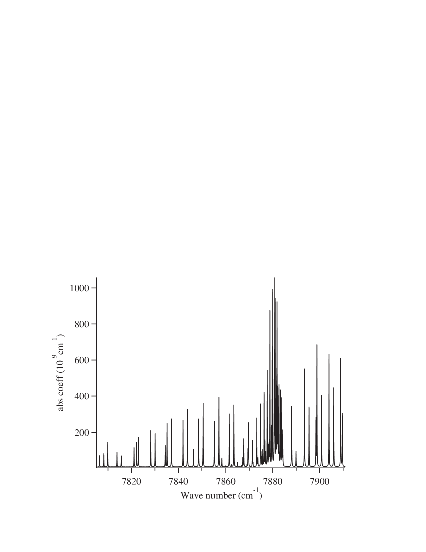
Figure 1: Overview of the transitions in the a${{}^{1}}{\triangle}_{g}{\leftarrow}$X ${}^{3}{\Sigma}^{-}_{g}$ band of oxygen recorded by CW-CRDS (P = 400 mbar, T= 300 K).

The overview of the transitions in the a${{}^{1}}{\triangle}_{g}{\leftarrow}$X ${}^{3}{\Sigma}^{-}_{g}$ band of oxygen is shown in Fig. 1. The transitions reported within this paper lie between 7640 to 7917 cm^-1 and it is clear that from the overview spectra that the line strength of these transitions are very low. We were able to measure only the symmetric isotopologues i.e. ¹⁶O₂ and ¹⁸O₂, since the line strengths for the transitions of asymmetric isotopologues are much lower than the resolution limit of our experimental set up.

3.1 Lines of ¹⁶O₂

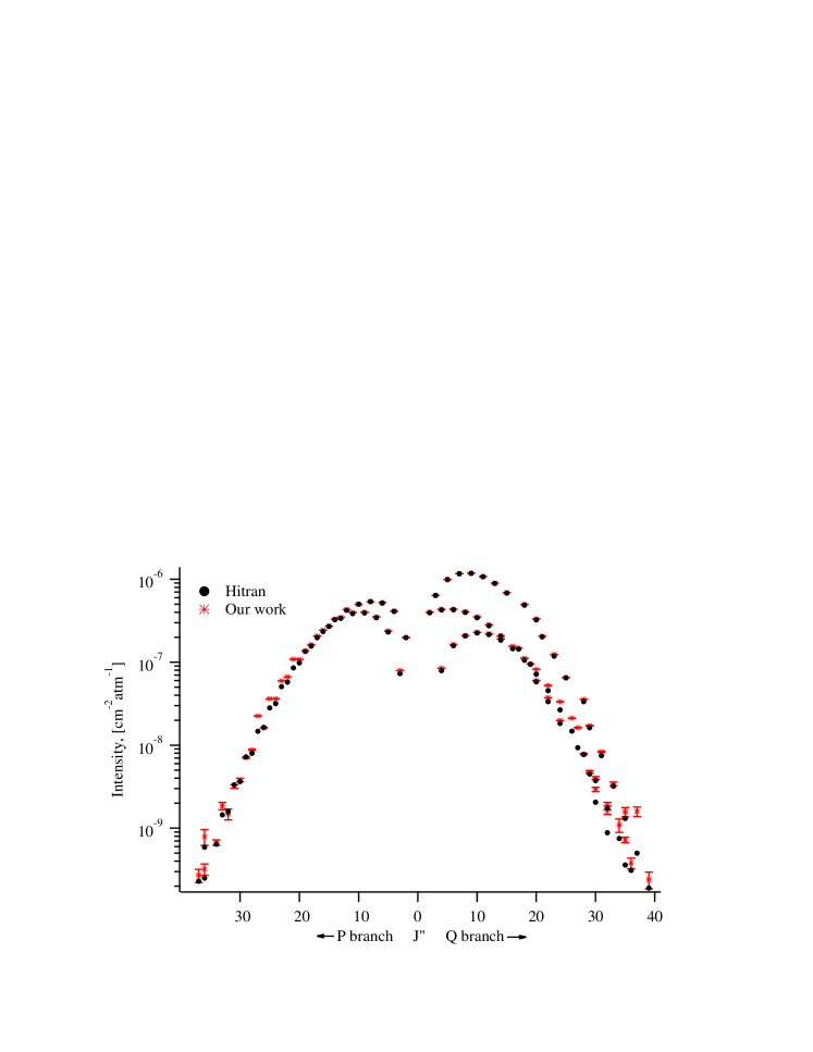
Figure 3: Intensity of the $P$, $Q$ branch of ¹⁶O₂.

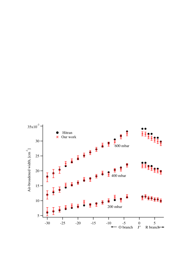
Figure 5: Width of $O$, $R$ branch ¹⁶O₂.

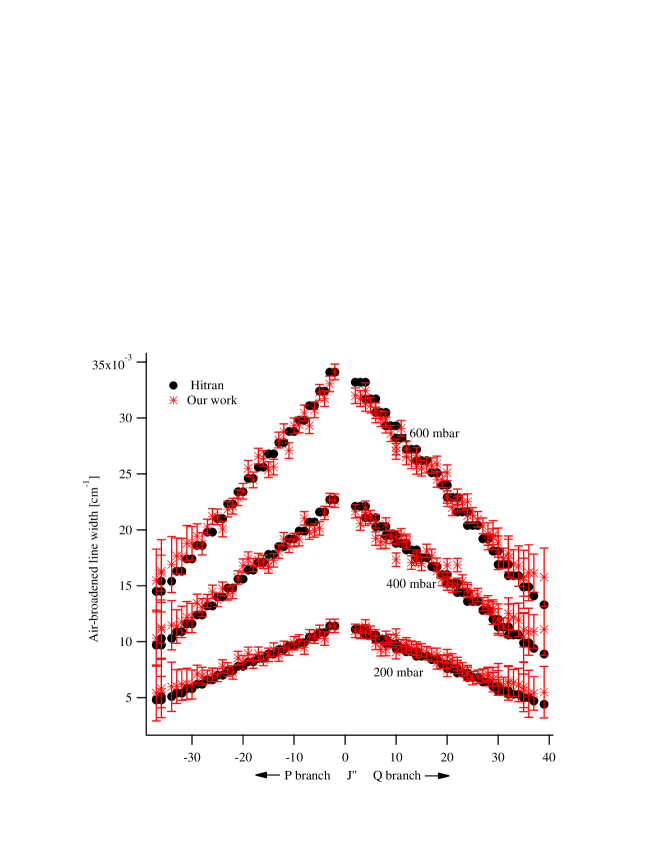
Figure 7: Width of $P$, $Q$ branch ¹⁶O₂.

We have measured 14 transitions in the $O$ branch, 7 transition in the $R$ branch, 36 transitions in the $P$ branch and 53 transition in the $Q$ branch of ¹⁶O₂ in the a${{}^{1}}{\triangle}_{g}{\leftarrow}$X ${}^{3}{\Sigma}^{-}_{g}$ $(0,0)$ band. Our measured parameters and corresponding experimental uncertainty of these transitions are given in Table 1, Table 2, Table LABEL:16O2Plineintensity and in Table LABEL:16O2Qlineintensity respectively. The uncertainties for some of the transitions are larger. Since many of the transitions overlap and hence the fitting become more difficult. In Fig. 3 and Fig. 3 we compared our measured line intensities for these transitions with the calculated values in the HITRAN database. Furthermore, we have measured the self-broadened linewidth (measurement with ultra pure oxygen sample) and the air-broadened linewidth (measurement with dry air sample) for these transitions at three different pressure i.e. 200 mbar, 400 mbar and 600 mbar which are shown in Fig. 5, Fig. 5 Fig. 7 and in Fig. 7 along with the calculated values in the HITRAN database. It is to be noted that, the measured line positions, line intensities, self-broadened and air-broadened Lorentzian half width are in good agreement with the predictions in the HITRAN database.

3.2 Lines of ¹⁸O₂

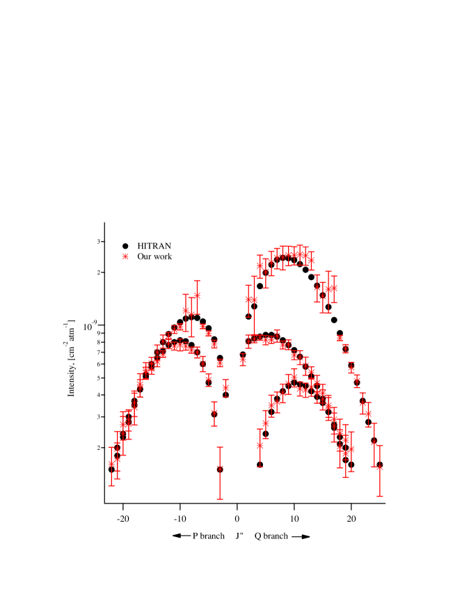
Figure 9: Intensity in the $P$, $Q$ branch of ¹⁸O₂.

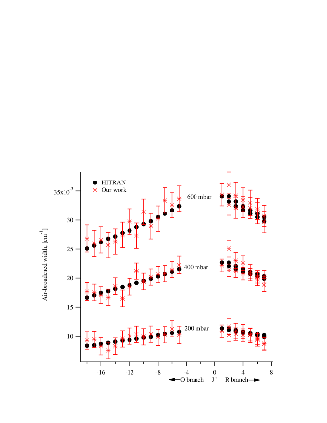
Figure 11: Width of $O$, $R$ branch ¹⁸O₂.

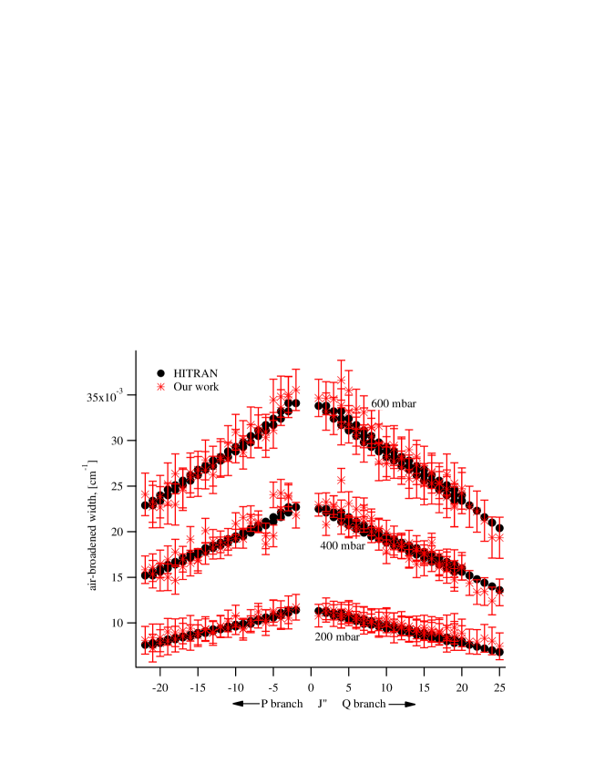
Figure 13: Width of $P$, $Q$ branch ¹⁸O₂.

We have measured 14 transitions in the $O$ branch,13 transition in the $R$ branch, 3 transition in the $S$ branch, 40 transitions in the $P$ branch, and 60 transition in the $Q$ branch of ¹⁸O₂ in the a${{}^{1}}{\triangle}_{g}{\leftarrow}$X ${}^{3}{\Sigma}^{-}_{g}$ $(0,0)$ band. Our measured parameters and corresponding experimental uncertainty of these transitions are given in Table 5, Table 6, Table LABEL:18O2Plineintensity and in Table LABEL:18O2Qlineintensity respectively. In Fig. 9, Fig. 9 we compared our measured line intensities for these transitions with the calculated values in the HITRAN database. Furthermore, we have measured the self-broadened linewidth (measurement with ultrapure oxygen sample) and the air-broadened linewidth (measurement with dry air sample) for these transitions at three different pressure i.e. 200 mbar, 400 mbar and 600 mbar which are shown in Fig. 11, Fig. 11 Fig. 13 and in Fig. 13 along with the calculated values in the HITRAN database. It is to be noted that, the measured line positions, line intensities, self-broadened and air-broadened Lorentzian half width are in good agreement with the predictions in the HITRAN database.

3.3 Data fitting

We used Matlab to perform a Voigt lineshape fit on each transition to a theoretical NICE-OHMS lineshape function [17]. The lineshape is accounts for the effect of the two levels of frequency modulation.

The energy of a transition from the ground state $(N^{{}^{\prime}},J^{{}^{\prime}})$ to the excited state $(J)$ is given by the equation

$$\tilde{\nu}_{J\leftarrow N^{{}^{\prime}},J^{{}^{\prime}}}=\tilde{\nu}_{0\leftarrow 0,0}+B{{}_{0}}J(J+1)-D_{0}[J(J+1)]^{2}-F^{{}^{\prime}}(N^{{}^{\prime}},J^{{}^{\prime}})$$ (1)

where the lower state energy $F^{{}^{\prime}}(N^{{}^{\prime}}J^{{}^{\prime}})$ is calculated with the molecular constant in a recent publication [1]. $\tilde{\nu}_{J\leftarrow N^{{}^{\prime}},J^{{}^{\prime}}}$ is the measured line position, and $\tilde{\nu}_{0\leftarrow 0,0}$, $B{{}_{0}}$ and $D_{0}$ are the molecular constants of the excited state, $a(\tilde{\nu}=0)$ which we measured.

3.3.1 ¹⁶O₂ parameters

We have measured 111 lines of the a${{}^{1}}{\triangle}_{g}{\leftarrow}$X ${}^{3}{\Sigma}^{-}_{g}$ $(0,0)$ band of ¹⁶O₂. To extract the parameters of each individual transition we fit Eq.1 to the line position of the measured transition. The results of the fit are given in Table 9, where the a${{}^{1}}{\triangle}_{g}$ state constants compared with those from Olaga [1], Amiot [19] and Rothman [20].

3.3.2 ¹⁸O₂ parameters

We have measured 130 lines of the a${{}^{1}}{\triangle}_{g}{\leftarrow}$X ${}^{3}{\Sigma}^{-}_{g}$ $(0,0)$ band of ¹⁸O₂. To extract the parameters of each individual transition we fit Eq.1 to the line position of the measured transition. The results of the fit are given in Table 10, where the a${{}^{1}}{\triangle}_{g}$ state constants compared with those from Olaga [1].

4 Conclusion

Our work characterized 241 ultraweak transitions in molecular oxygen by measuring their line positions, self-broadened and air-broadened linewidths and line intensities using NICE-OHMS. The precise value of the parameters provide a path to improve the existing HITRAN database. It is to be noted that the a${{}^{1}}{\triangle}_{g}{\leftarrow}$X ${}^{3}{\Sigma}^{-}_{g}$ electric quadrupole transitions of ¹⁶O₂ and ¹⁸O₂ are important to atmospheric modelling. The NICE-OHMS measurement of different a${{}^{1}}{\triangle}_{g}{\leftarrow}$X ${}^{3}{\Sigma}^{-}_{g}$ transitions in this work provide one of the best set of spectroscopic parameters for the a${{}^{1}}{\triangle}_{g}$ state of ¹⁶O₂ and ¹⁸O₂.

5 Acknowledgements

We are grateful to Tzahi Grunzweig for his help with labview for automation of the experiment. This research is supported by the New Zealand Foundation for Research, Science and Technology, Otago University.

Table 1: Measured transition parameters of the $O$ branch of ¹⁶O₂.

Transition	Position		Line intensity	Self-broadened half-width
$\Delta$ N N′ $\Delta$ J J′	cm-1		10-8cm-2atm-1	cm-1 at 400 mbar
O31P30	7692.459(2)		0.139(18)	0.0136(14)
O29P28	7706.069(2)		0.338(10)	0.0140(12)
O27P26	7719.552(2)		0.722(14)	0.0144(9)
O25P24	7732.894(2)		1.372(11)	0.0155(6)
O23P22	7746.031(2)		3.062(10)	0.0163(6)
O21P20	7759.092(2)		5.125(10)	0.0167(6)
O19P18	7772.052(2)		7.369(10)	0.0167(6)
O17P16	7784.807(2)		10.173(10)	0.0175(6)
O15P14	7797.435(2)		13.147(10)	0.0179(6)
O13P12	7809.917(2)		16.335(10)	0.0186(6)
O11P10	7822.243(2)		18.934(10)	0.0194(6)
O9P8	7834.445(2)		18.041(10)	0.0198(6)
O7P6	7846.459(2)		14.563(10)	0.0202(6)
O5P4	7858.330(2)		8.204(10)	0.0214(6)

Table 2: Measured transition parameters of the $R$ and $S$ branch of ¹⁶O₂.

Transition	Position		Line intensity	Self-broadened half width
$\Delta$ N N′ $\Delta$ J J′	cm-1		10-8cm-2atm-1	cm-1 400 mbar
R1R1	7888.092(2)		71.688(10)	0.0222(6)
R1Q2	7889.930(2)		18.870(10)	0.0222(6)
R3R3	7893.558(2)		82.862(10)	0.0210(6)
R3Q4	7895.457(2)		41.828(10)	0.0210(6)
R5R5	7898.879(2)		88.711(10)	0.0198(6)
R5Q6	7900.841(2)		58.952(10)	0.0198(6)
R7R7	7904.023(2)		91.036(10)	0.0194(6)
S1R2	7898.470(2)		37.062(10)	0.0214(6)

Table 3: Measured transition parameters of the $P$ branch of ¹⁶O₂.

Transition	Position	Line intensity	Self-broadened half-width
$\Delta$ N N′ $\Delta$ J J′ V	cm-1	10-8cm-2atm-1	cm-1 at 400 mbar
P37P37	7750.151(2)	0.037(5)	0.0119(25)
P37Q36	7751.843(2)	0.032(5)	0.0120(16)
P35P36	7758.676(2)	0.209(17)	0.0120(14)
P35Q34	7760.315(2)	0.067(5)	0.0127(22)
P33P33	7767.024(2)	0.186(19)	0.0133(15)
P33Q32	7768.760(2)	0.148(22)	0.0126(14)
P31P31	7775.219(2)	0.318(17)	0.0139(14)
P31Q30	7776.958(2)	0.381(18)	0.0137(13)
P29P29	7783.193(2)	0.711(14)	0.0148(8)
P29Q28	7785.02(2)	0.878(13)	0.0149(8)
P27P27	7791.141(2)	2.251(10)	0.0149(6)
P27Q26	7792.931(2)	1.622(10)	0.0156(6)
P25P25	7798.861(2)	3.629(10)	0.0146(6)
P25Q24	7800.622(2)	3.631(10)	0.0148(6)
P23P23	7806.475(2)	5.960(10)	0.0157(6)
P23Q22	7808.213(2)	6.657(10)	0.0158(6)
P21P21	7813.861(2)	10.867(10)	0.0164(6)
P21Q20	7815.716(2)	10.859(10)	0.0170(6)
P19P19	7821.099(2)	13.731(10)	0.0177(6)
P19Q18	7822.939(2)	16.290(10)	0.0171(6)
P17P17	7828.202(2)	20.672(10)	0.0177(6)
P17Q16	7830.106(2)	24.296(10)	0.0174(6)
P15P15	7835.216(2)	27.187(10)	0.0167(6)
P15Q14	7837.104(2)	33.127(10)	0.0179(6)
P13P13	7841.963(2)	34.795(10)	0.0183(6)
P13Q12	7843.927(2)	42.831(10)	0.0189(6)
P11P11	7848.657(2)	39.733(10)	0.0193(6)
P11Q10	7850.604(2)	49.796(10)	0.0192(6)
P9P9	7855.182(2)	40.231(10)	0.0195(6)
P9Q8	7857.122(2)	53.482(10)	0.0196(6)
P7P7	7861.503(2)	35.064(10)	0.0197(6)
P7Q6	7863.463(2)	52.423(10)	0.0199(6)
P5P5	7867.711(2)	23.739(10)	0.0205(6)
P5Q4	7869.706(2)	41.412(10)	0.0209(6)
P3P3	7873.700(2)	7.952(10)	0.0227(6)
P3Q2	7875.785(2)	19.828(10)	0.0219(6)

Table 4: Measured transition parameters of the $Q$ branch of ¹⁶O₂.

Transition	Position	Line intensity	Self-broadened half-width
$\Delta$ N N′ $\Delta$ J J′ V	cm-1	10-8cm-2atm-1	cm-1 at 400 mbar
Q3R2	7884.298(2)	40.095(10)	0.0219(6)
Q3Q3	7882.217(2)	64.156(10)	0.0212(6)
Q3P4	7884.141(2)	8.482(10)	0.0211(6)
Q5R4	7883.870(2)	43.470(10)	0.0203(6)
Q5Q5	7881.834(2)	99.431(10)	0.0202(6)
Q5P6	7883.822(2)	16.293(10)	0.0197(6)
Q7R6	7883.285(2)	43.599(10)	0.0203(6)
Q7Q7	7881.326(2)	116.910(10)	0.0194(6)
Q7P8	7883.318(2)	20.976(10)	0.0205(6)
Q9R8	7882.631(2)	40.629(10)	0.0196(6)
Q9Q9	7880.664(2)	118.606(10)	0.0200(6)
Q9P10	7882.704(2)	22.926(10)	0.0196(6)
Q11R10	7881.713(2)	35.100(10)	0.0184(6)
Q11Q11	7879.818(2)	107.894(10)	0.0188(6)
Q11P12	7881.892(2)	22.012(10)	0.0194(6)
Q13R12	7880.716(2)	28.214(10)	0.0182(6)
Q13Q13	7878.812(2)	89.421(10)	0.0177(6)
Q13P14	7880.908(2)	19.084(10)	0.0181(6)
Q15R14	7879.564(2)	20.762(10)	0.0183(6)
Q15Q15	7877.646(2)	68.931(10)	0.0172(6)
Q15P16	7879.798(2)	15.592(10)	0.0189(6)
Q17R16	7878.227(2)	14.756(10)	0.0174(6)
Q17Q17	7876.317(2)	49.824(10)	0.0172(6)
Q17P18	7878.490(2)	11.131(10)	0.0178(6)
Q19R18	7876.714(2)	9.569(10)	0.0169(6)
Q19Q19	7874.846(2)	33.174(10)	0.0176(6)
Q19P20	7877.008(2)	8.197(10)	0.0174(6)
Q21R20	7875.053(2)	6.005(10)	0.0167(6)
Q21Q21	7873.214(2)	20.530(10)	0.0162(6)
Q21P22	7875.399(2)	5.245(10)	0.0168(6)
Q23R22	7873.172(2)	3.728(10)	0.0166(6)
Q23Q23	7871.393(2)	12.400(10)	0.0162(6)
Q23P24	7873.571(2)	3.341(10)	0.0153(6)
Q25R24	7871.260(2)	1.981(10)	0.0155(6)
Q25Q25	7869.429(2)	6.520(10)	0.0150(6)
Q25P26	7871.593(2)	2.112(10)	0.0151(6)
Q27R26	7869.050(2)	1.628(10)	0.0149(6)
Q27Q27	7867.299(2)	3.566(10)	0.0147(6)
Q27P28	7869.517(2)	0.783(13)	0.0146(8)
Q29R28	7866.741(2)	0.476(16)	0.0141(11)
Q29Q29	7865.008(2)	1.717(10)	0.0144(6)
Q29P30	7867.212(2)	0.401(16)	0.0139(11)
Q31R30	7864.257(2)	0.293(18)	0.0135(14)
Q31Q31	7862.492(2)	0.833(12)	0.0135(8)
Q31P32	7864.728(2)	0.186(19)	0.0145(14)
Q33R32	7861.57(2)	0.165(19)	0.0133(15)
Q33Q33	7859.856(2)	0.342(17)	0.0139(12)
Q33P34	7862.130(2)	0.109(20)	0.0139(15)
Q35R35	7858.739(2)	0.072(6)	0.0101(22)
Q35Q35	7857.004(2)	0.157(20)	0.0120(15)
Q35P36	7859.310(2)	0.038(6)	0.0126(21)
Q37Q37	7853.988(2)	0.159(21)	0.0129(15)
Q39Q39	7850.825(2)	0.064(7)	0.0127(23)

Table 5: Measured transition parameters of the $O$ branch of ¹⁸O₂.

Transition	Position		Line intensity	Self-broadened half-width
$\Delta$ N N′ $\Delta$ J J′ V	cm-1		10-8cm-2atm-1	cm-1 at 400 mbar
O19P18	7779.627(2)		0.013(5)	0.0171(15)
O18P17	7785.657(2)		0.021(5)	0.0176(14)
O17P16	7791.669(2)		0.022(5)	0.0183(15)
O16P15	7797.647(2)		0.025(5)	0.0177(15)
O15P14	7803.528(2)		0.033(5)	0.0177(14)
O14P13	7809.441(2)		0.027(4)	0.0193(15)
O13P12	7815.363(2)		0.043(4)	0.0193(14)
O12P11	7821.190(2)		0.042(4)	0.0186(14)
O11P10	7827.009(2)		0.039(5)	0.0202(14)
O10P9	7832.777(2)		0.042(3)	0.0195(14)
O9P8	7838.509(2)		0.032(4)	0.0195(14)
O8P7	7844.231(2)		0.042(4)	0.0204(14)
O7P6	7849.877(2)		0.035(4)	0.0212(14)
O6P5	7855.489(2)		0.029(5)	0.0212(14)

Table 6: Measured transition parameters of the $R$ and $S$ branch of ¹⁸O₂.

Transition	Position		Line intensity	Self-broadened half-width
$\Delta$ N N′ $\Delta$ J J′ V	cm-1		10-8cm-2atm-1	cm-1 at 400 mbar
R1R1	7889.051(2)		0.151(32)	0.0230(11)
R1Q2	7890.971(2)		0.036(5)	0.0219(14)
R2R2	7891.679(2)		0.191(31)	0.0222(11)
R2Q3	7893.593(2)		0.056(4)	0.0215(14)
R3R3	7894.221(2)		0.191(30)	0.0219(11)
R3Q4	7896.199(2)		0.082(4)	0.0215(12)
R4R4	7896.781(2)		0.221(31)	0.0211(11)
R4Q5	7898.773(2)		0.097(4)	0.0210(12)
R5R5	7899.278(2)		0.300(32)	0.0204(11)
R5Q6	7901.264(2)		0.238(35)	0.0211(11)
R6R6	7901.729(2)		0.198(31)	0.0206(11)
R6Q7	7903.717(2)		0.253(32)	0.0204(11)
R7R7	7904.157(2)		0.247(30)	0.0204(11)
S0R1	7893.632(2)		0.059(4)	0.0225(12)
S1R2	7899.001(2)		0.070(4)	0.0219(12)
S2R3	7904.325(2)		0.076(4)	0.0214(12)

Table 7: Measured transition parameters of the $P$ branch of ¹⁸O₂.

Transition	Position	Line intensity	Self-broadened half-width
$\Delta$ N N′ $\Delta$ J J′ V	cm-1	10-8cm-2atm-1	cm-1 at 400 mbar
P22P22	7815.521(2)	0.016(4)	0.0170(15)
P22Q21	7817.345(2)	0.017(4)	0.0168(15)
P21P21	7818.981(2)	0.020(5)	0.0171(15)
P21Q20	7820.831(2)	0.024(6)	0.0170(15)
P20P20	7822.459(2)	0.027(5)	0.0166(15)
P20Q19	7824.258(2)	0.027(5)	0.0179(15)
P19P19	7825.796(2)	0.029(4)	0.0177(15)
P19Q18	7827.690(2)	0.034(7)	0.0184(15)
P18P18	7829.210(2)	0.036(6)	0.0174(14)
P18Q17	7831.084(2)	0.044(5)	0.0182(14)
P17P17	7832.571(2)	0.046(7)	0.0177(14)
P17Q16	7834.393(2)	0.055(6)	0.0181(14)
P16P16	7835.876(2)	0.054(4)	0.0170(14)
P16Q15	7837.756(2)	0.056(4)	0.0190(12)
P15P15	7839.164(2)	0.061(5)	0.0188(14)
P15Q14	7841.035(2)	0.070(7)	0.0180(12)
P14P14	7842.343(2)	0.062(4)	0.0182(14)
P14Q13	7844.284(2)	0.081(7)	0.0182(12)
P13P13	7845.528(2)	0.068(3)	0.0191(14)
P13Q12	7847.487(2)	0.087(4)	0.0193(12)
P12P12	7848.723(2)	0.078(5)	0.0189(12)
P12Q11	7850.656(2)	0.095(5)	0.0195(10)
P11P11	7851.817(2)	0.076(4)	0.0197(12)
P11Q10	7853.783(2)	0.098(4)	0.0198(10)
P10P10	7854.912(2)	0.077(6)	0.0193(12)
P10Q9	7856.884(2)	0.121(29)	0.0197(9)
P9P9	7858.003(2)	0.076(4)	0.0191(12)
P9Q8	7859.914(2)	0.115(29)	0.0190(9)
P8P8	7861.020(2)	0.072(3)	0.0206(12)
P8Q7	7862.962(2)	0.147(32)	0.0207(9)
P7P7	7863.980(2)	0.070(5)	0.0207(13)
P7Q6	7865.945(2)	0.098(3)	0.0198(12)
P6P6	7866.943(2)	0.060(6)	0.0222(14)
P6Q5	7868.863(2)	0.090(3)	0.0214(12)
P5P5	7869.786(2)	0.049(4)	0.0203(14)
P5Q4	7871.769(2)	0.078(4)	0.0213(12)
P4P4	7872.687(2)	0.032(5)	0.0211(15)
P4Q3	7874.676(2)	0.061(3)	0.0210(12)
P3P3	7875.457(2)	0.015(5)	0.0223(15)
P3Q2	7877.569(2)	0.044(5)	0.0229(14)

Table 8: Measured transition parameters of the $Q$ branch of ¹⁸O₂.

Transition	Position	Line intensity	Self-broadened half-width
$\Delta$ N N′ $\Delta$ J J′ V	cm-1	10-8cm-2atm-1	cm-1 at 400 mbar
Q2R1	7885.814(2)	0.064(5)	0.0223(12)
Q2Q2	7883.661(2)	0.140(29)	0.0216(10)
Q3R2	7885.623(2)	0.081(7)	0.0219(12)
Q3Q3	7883.539(2)	0.139(51)	0.0214(10)
Q3P4	7885.485(2)	0.021(5)	0.0200(13)
Q4R3	7885.414(2)	0.083(4)	0.0211(12)
Q4Q4	7883.378(2)	0.218(33)	0.0216(10)
Q4P5	7885.322(2)	0.028(5)	0.0206(13)
Q5R4	7885.216(2)	0.085(3)	0.0212(12)
Q5Q5	7883.168(2)	0.201(38)	0.0217(10)
Q5P6	7885.191(2)	0.035(5)	0.0200(13)
Q6R5	7884.96(2)	0.082(5)	0.0206(12)
Q6Q6	7882.980(2)	0.227(36)	0.0202(10)
Q6P7	7884.975(2)	0.037(5)	0.0203(13)
Q7R6	7884.664(2)	0.083(4)	0.0210(12)
Q7Q7	7882.689(2)	0.242(32)	0.0190(10)
Q7P8	7884.695(2)	0.041(5)	0.0201(13)
Q8R7	7884.331(2)	0.087(7)	0.0195(12)
Q8Q8	7882.443(2)	0.245(38)	0.0192(10)
Q8P9	7884.394(2)	0.046(6)	0.0197(13)
Q9R8	7884.052(2)	0.077(4)	0.0196(12)
Q9Q9	7882.072(2)	0.250(32)	0.0198(10)
Q9P10	7884.124(2)	0.050(6)	0.0198(13)
Q10R9	7883.598(2)	0.078(5)	0.0188(12)
Q10Q10	7881.699(2)	0.250(30)	0.0200(10)
Q10P11	7883.744(2)	0.043(4)	0.0201(13)
Q11R10	7883.19(2)	0.068(4)	0.0196(13)
Q11Q11	7881.273(2)	0.253(33)	0.0197(10)
Q11P12	7883.342(2)	0.043(4)	0.0194(13)
Q12R11	7882.734(2)	0.065(6)	0.0184(13)
Q12Q12	7880.819(2)	0.249(30)	0.0190(10)
Q12P13	7882.927(2)	0.044(5)	0.0191(14)
Q13R12	7882.263(2)	0.059(7)	0.0186(13)
Q13Q13	7880.326(2)	0.234(28)	0.0194(10)
Q13P14	7882.433(2)	0.041(5)	0.0182(14)
Q14R13	7881.726(2)	0.054(4)	0.0184(13)
Q14Q14	7879.845(2)	0.165(29)	0.0181(10)
Q14P15	7881.898(2)	0.038(5)	0.0183(14)
Q15R14	7881.138(2)	0.047(5)	0.0180(13)
Q15Q15	7879.247(2)	0.147(29)	0.0181(10)
Q15P16	7881.361(2)	0.034(5)	0.0178(14)
Q16R15	7880.536(2)	0.041(5)	0.0181(14)
Q16Q16	7878.644(2)	0.160(43)	0.0167(10)
Q16P17	7880.767(2)	0.027(5)	0.0178(14)
Q17R16	7879.864(2)	0.035(5)	0.0172(15)
Q17Q17	7878.009(2)	0.163(28)	0.0176(10)
Q17P18	7880.122(2)	0.024(5)	0.0175(14)
Q18R17	7879.166(2)	0.029(5)	0.0175(15)
Q18Q18	7877.326(2)	0.085(3)	0.0174(12)
Q18P19	7879.414(2)	0.022(5)	0.0174(15)
Q19R18	7878.482(2)	0.020(5)	0.0174(15)
Q19Q19	7876.581(2)	0.073(4)	0.0178(12)
Q19P20	7878.708(2)	0.020(5)	0.0168(15)

Table 9: Comparison of molecular constants in cm^-1 of the $\nu$ = 0 levels of the a${{}^{1}}{\triangle}_{g}$ state of ¹⁶O₂.

Constants	This work	Olaga [1]	Amiot [19]	Rothman [20]
$\tilde{\nu}_{0\leftarrow 0,0}$	7883.756662(142)	7883.756645(113)	7883.76179(28)	7882.4288(3)
$B{{}_{0}}$	1.417832166 (66)	1.417839039 (38)	1.41784020(82)	1.4178442(19)
$D{{}_{0}}\times$ 10-6	5.102159(351)	5.102256(243)	5.1074(24)	5.11144(139)

Table 10: Comparison of molecular constants in cm^-1 of the $\nu$ = 0 levels of the a${{}^{1}}{\triangle}_{g}$ state of ¹⁸O₂.

Constants	This work	Olaga [1]
$\tilde{\nu}_{0\leftarrow 0,0}$	7886.512585(200)	7886.409277(117)
$B{{}_{0}}$	1.260406188(110)	1.260409499 (56)
$D{{}_{0}}\times$ 10-6	4.011059(850)	4.029678(664)

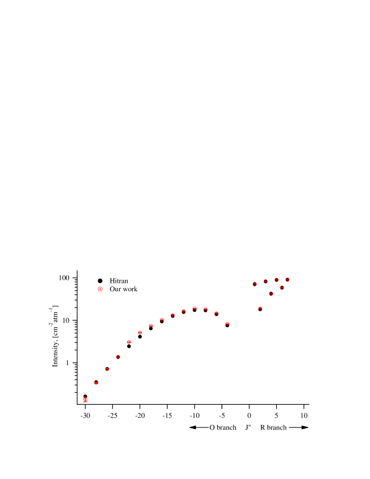
Figure 2: Intensity of the $O$, $R$ branch of ¹⁶O₂.

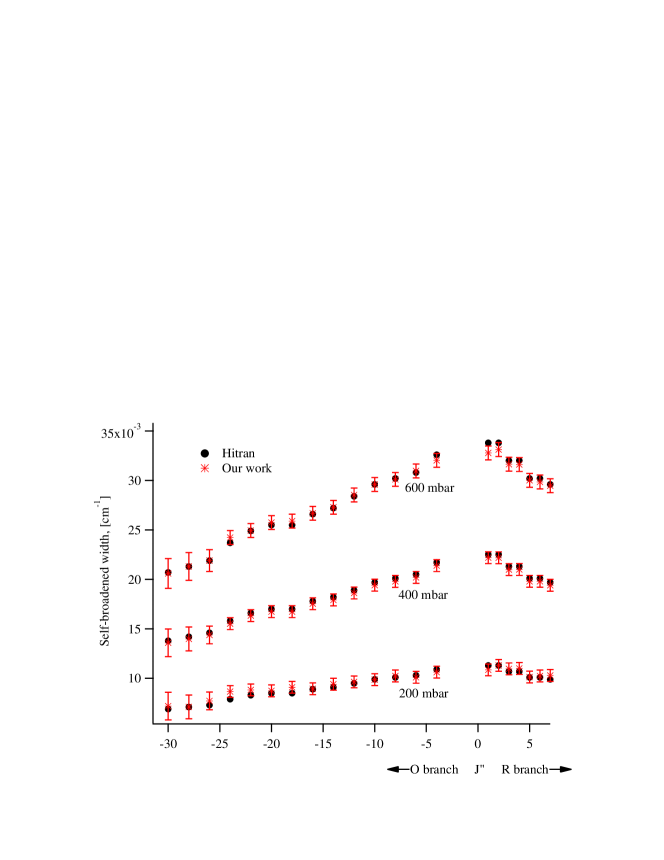
Figure 4: Width of $O$, $R$ branch ¹⁶O₂.

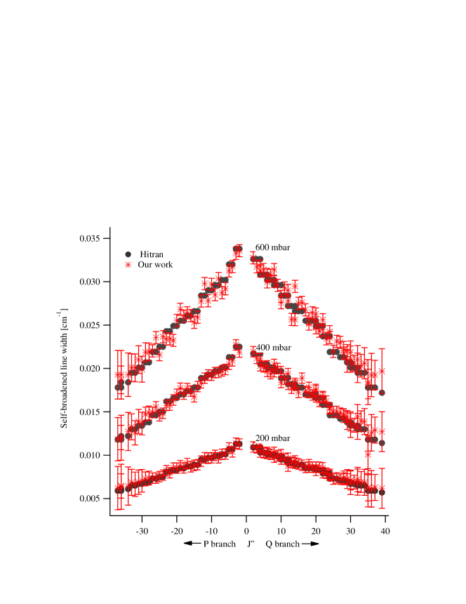
Figure 6: Width of $P$, $Q$ branch ¹⁶O₂.

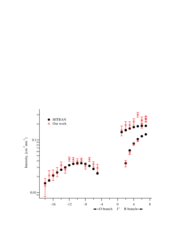
Figure 8: Intensity of the $O$, $R$ branch of ¹⁸O₂.

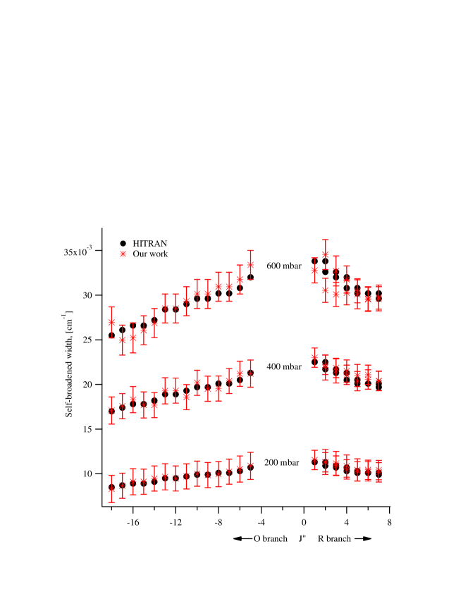
Figure 10: Width of $O$, $R$ branch ¹⁸O₂.

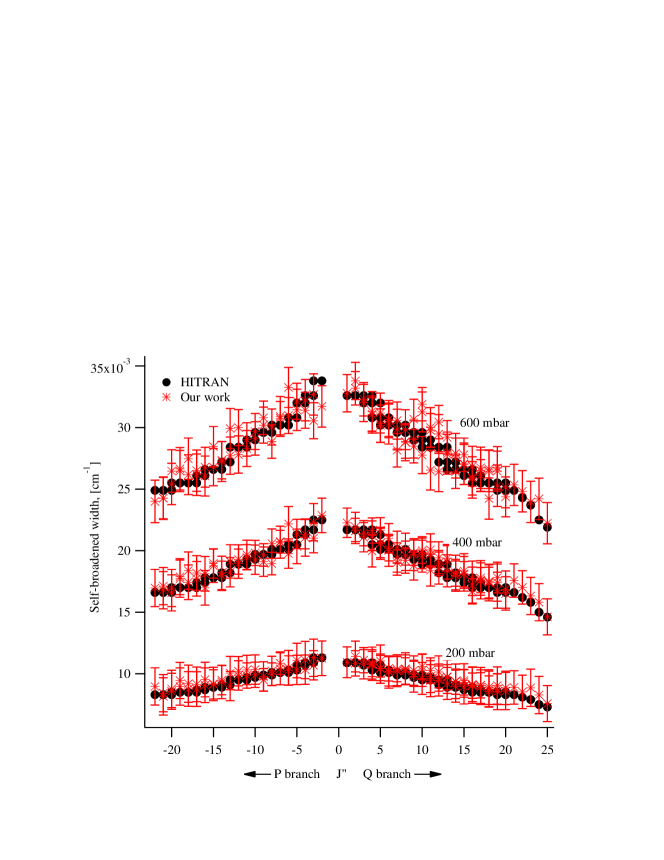
Figure 12: Width of $P$, $Q$ branch ¹⁸O₂.

References

- [1] O. Leshchishina, S. Kassi, I.E. Gordon, L.S. Rothman, L. Wang, A. Campargue, High sensitivity CRDS of the aX band of oxygen near 1.27 m: Extended observations, quadrupole transitions, hot bands and minor isotopologues, J. Quant. Spec. Rad. Trans. 111 (2010) 2236 2245.
- [2] R.A. Washenfelder, G.C. Toon, J.F. Blavier, N.T. Allen, P.O. Wennberg, et al. Carbon dioxide column abundances at the Wisconsin Tall Tower site. J. Geophys. Res. 111 (2006) 22305.
- [3] L.S. Rothman, I.E. Gordon, A. Barbe, D.C. Benner, P.F. Bernath, M. Brik et al. The HITRAN 2008 molecular spectroscopic database. J. Quant. Spectrosc. Radiat. Transfer. 110 (2009) 533-72.
- [4] W.J. Lafferty, A.M. Solodov, C.L. Lugez, G.T. Fraser, Rotational line strength and self-pressure-broadening coefficients for the 1.27 m aX band of O2. Appl. Opt. 37 (1998) 2264-70.
- [5] S.M. Newman, I.C. Lane, A.J. Orr-Ewing, D.A. Newmham, J. Ballard, Integrated absorption intensity and einstein coefficients for the O2 aX transitons: a comparison of cavity ringdown and high resolution Fourier transformation spectroscpy with a long path absorption cell. J Chem. Phys. 110 (1999) 10749-57.
- [6] I.E. Gordon, S. Kassi, A. Campergue, G.C. Toon, First identification of the aX electric quadrupole transition of oxygen in the solar and laboratory spectra. J. Quant. Spectrosc. Radiat. Transfer. 111 (2010) 1174-83.
- [7] G. Rouilli, G. Millot, R. Saint-Loup, H. Berger, High-resolution stimulated Raman spectroscopy. J. Mol. Spectrosc. 154 (1992) 372-82.
- [8] K.W. Hillig, C.C.W. Chiu, W.G. Read, E.A. Cohen, The pure rotation spectrum of a O2. J. Mol. Spectrosc. 109 (1985) 205-6.
- [9] R.R. Gamache, A. Goldman, L.S. Rothman, Improved spectral parameters for the three most abundant isotopomers of the oxygen molecule. J. Quant. Spectrosc. Radiat. Transfer. 59 (1998) 495-509.
- [10] P.H. Krupenie, The spectrum of molecular oxygen. J. Phys. Chem. Ref. Data. 1 (1972) 423-534.
- [11] J. Brualt, Private Communication (1982) .
- [12] M. Mizushima, S. Yamamoto, Microwave absorption lines of 16O86O in its (, =0) state. J. Mol. Spectrosc. 148 (1991) 447-52.
- [13] L. Herzberg, G. Herzberg, Fine structure of the infrared atomospheric oxygen bands. J. Astrophys. 105 (1947) 353.
- [14] S-L. Cheah, Y-P. Lee, J.F. Ogilvie, Wavenumber, strength, widths and shift with pressure of lines in four bands of gaseous 16O2 in the systems aX and bX . J. Quant. Spectrosc. Radiat. Transfer. 64 (2000) 467-82.
- [15] J. Ye, L.S. Ma, J.L. Hall, Ultrasensitive detections in atomic and molecular physics: demonstration in molecular overtone spectros- copy, J. Opt. Soc. Am. B-Opt. Phys. 15 (1) (1998) 6 15.
- [16] L.S. Ma, J. Ye, P. Dube, J.L. Hall, Ultrasensitive frequency modulation spectroscopy enhanced by a high-finesse optical cavity: theory and application to overtone transitions of C2H2 and C2HD, J. Opt. Soc. Am. B Opt. Phys. 16 (12) (1999) 2255 - 2268.
- [17] N.J. van Leeuwen, A.C. Wilson, Spectroscopic measurement of pressure-broadened ultra-weak molecular transitions using NICE- OHMS, J. Opt. Soc. Am. B Opt. Phys. 21 (10) (2004) 1713 - 1721.
- [18] B.V. Perevalov, S. Kassi, D. Romanini, V.I. Perevalov, S.A. Tashkun, A. Camparague, CW-cavity ringdown spectroscopy of carbon dioxide isotopologues near 15. m. J. Mol. Spectrosc. 238 (2006) 241 - 55.
- [19] C. Amiot, J. Vergès, The magnetic dipole aX and bX transition in the oxygen afterglow. Can. J. Phys. 59 (1981) 1391.
- [20] L.S. Rothman, Magnetic dipole infrared atmospheric oxygen bands. Appl. Opts. 21 (1982) 24281-31.