Single top quark differential decay rate formulae including detector effects

Abstract

Since the discovery of parity violation in 1957, angular distributions of leptons coming from the weak decay of polarized fermions have been used to probe the structure of the $Wqq^{\prime}$ vertex. Vector and axial vector couplings reveal themselves in the angular distributions of both light and heavy polarized fermions, but tensor and pseudotensor couplings have a prominent influence on the angular distributions only for fermions heavier than the $W$ boson; i.e. the top quark. The copious $t$-channel production of polarized single top quarks at the LHC provides an opportunity to study the angular distributions of leptons from polarized top quark decay. In this paper we develop formulae for differential rates intended to be used as a likelihood function in the simultaneous extraction of decay amplitudes, phases, and polarization. The incorporation of detector effects in these formulae is accomplished using a variant of the familiar convolution theorem applying to a decomposition of the differential rates in spherical harmonics.

1 Introduction

Among the six known quarks of the Standard Model (SM), the top quark is unique in having a large mass, 173.2$\pm$0.9 GeV ref:TeVAverage , which is about 35 times as large as the next heavy quark, twice as large as the $W$ boson, and close the to the electroweak symmetry breaking scale $\Lambda_{EW}=1/(\sqrt{2}G_{F})\approx$ 246 GeV, where $G_{F}$ is the Fermi constant. The large mass of the top quark may be a remnant of couplings between the top quark and new physics at a higher mass scale. The new physics can be described by an effective Lagrangian, and one of its effects is to modify the structure of the $Wtb$ vertex. In the SM the $Wtb$ vertex is described by the coupling

$${\cal L}_{Wtb}=-\frac{g}{\sqrt{2}}{\bar{b}}\gamma^{\mu}\frac{1}{2}\left(1-\gamma^{5}\right)tW^{-}_{\mu}+\text{h.c.}$$

Radiative corrections to the vertex can be absorbed into a small number of nonrenormalizable effective couplings called anomalous couplings, as follows:

$${\cal L}_{Wtb}=-\frac{g}{\sqrt{2}}{\bar{b}}\gamma^{\mu}\left(V_{L}P_{L}+V_{R}P_{R}\right)tW^{-}_{\mu}-\frac{g}{\sqrt{2}}{\bar{b}}\frac{i\sigma^{\mu\nu}}{M_{W}}q_{\nu}\left(g_{L}P_{L}+g_{R}P_{R}\right)tW^{-}_{\mu}+\text{h.c.}$$

In this expression, $P_{L}\equiv\frac{1}{2}(1-\gamma^{5})$ and $P_{R}\equiv\frac{1}{2}(1+\gamma^{5})$ are the left and right-handed projection operators, $V_{L}$, $V_{R}$, $g_{L}$, and $g_{R}$ are complex coupling constants which all (except for $V_{L}$) vanish in the SM, and $q$ is the four-momentum transfer at the $Wtb$ vertex. Imaginary components of any of coupling constants are particularly interesting since they signal new sources of $CP$ violation, beyond the single phase in the CKM matrix which is presently the only known source.

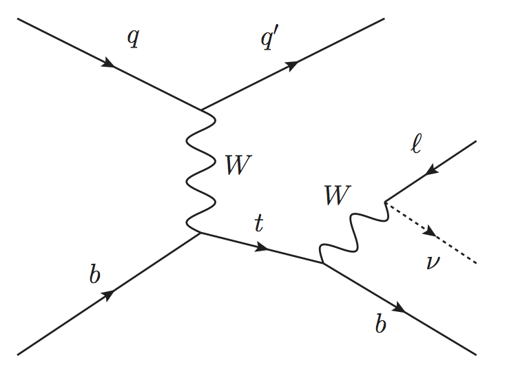
Figure 1: $t$-channel production of single top quarks in $pp$ collisions.

The couplings influence the angular distribution of top quark decay products as described in ref. AguilarSaavedra:2010wpol . We shall be mainly interested in $t$-channel single quark production and decay at the LHC, illustrated in Fig. 1. Experimentally one can detect and fully reconstruct the decay $t\rightarrow W^{+}b$; $W^{+}\rightarrow l^{+}\nu$ and measure the momentum of the spectator jet. The neutrino in the decay can be reconstructed from missing transverse energy in a “hermetic” detector covering a solid angle of approximately 4$\pi$. The coordinate system in which we describe the decay kinematics is as follows. The momentum of the $W$ boson in the top quark rest frame is called ${\vec{q}}$ and the spectator quark jet direction, which we take as polarization axis of the top quark is called ${\vec{s}}_{t}$. Two other directions in space orthogonal to ${\vec{q}}$ are meaningful as proposed in ref. AguilarSaavedra:2010wpol and described Fig. 2:

$${\vec{N}} = {\vec{s}}_{t}\times{\vec{q}}\,,$$

$${\vec{T}} = {\vec{q}}\times{\vec{N}}\,.$$

Using these directions we can construct a right-handed coordinate system such that the ${\hat{x}}$ direction points along $-{\vec{T}}$; the ${\hat{y}}$ direction lies along $\vec{N}$, and the ${\hat{z}}$ direction points along ${\vec{q}}$. We define $\theta$ as the angle between ${\vec{s}}_{t}$ and ${\vec{q}}$ in the top quark rest frame. The momentum of the charged lepton as measured in the $W$ rest frame is called $\vec{p_{l}}$. In this paper we analyze the distribution of polar and azimuthal helicity angles, $\theta^{*}$ and $\phi^{*}$, of that lepton in this coordinate system. The main objective is to obtain normalized analytic expressions describing the probability densities in angular variables, parametrized in terms of observable physics quantities (to be defined below), which incorporate detector effects. The purpose of these expressions is that they can then be used with reconstructed collider data to build a likelihood function in a multidimensional space of relevant physics parameters. A variety of more or less well-known techniques use the likelihood function to draw inferences on the physics parameters. These techniques include the unbinned maximum likelihood fit, the Feldman-Cousins method feldmanCousins , and Bayesian inference using Markov chain Monte Carlo.

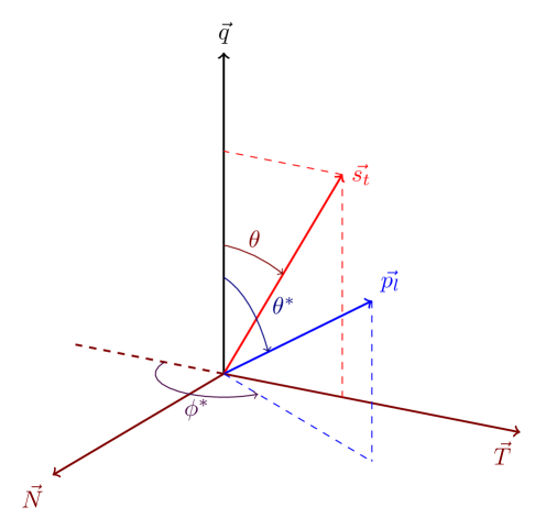
Figure 2: The coordinate system used for the analysis of polarized single top quarks produced in the $t$-channel. A Cartesian coordinate system is defined by the $\left\{-{\vec{T}},\vec{N},{\vec{q}}\right\}$ directions. The angles $\theta$, $\theta^{*}$ and $\phi^{*}$ are defined in the text.

2 Differential decay rates for polarized single top quark

We construct the angular dependence of the decay $t\to W^{+}b;W^{+}\to l^{+}\nu$ using the helicity formalism Richman:1984gh . The angular dependence of the amplitude for two-body decay is given by

$$A(a\to f)=\left[\frac{2J+1}{4\pi}\right]^{\frac{1}{2}}{D^{J}_{M,\lambda}}^{*}(\varphi,\theta,-\varphi)A_{\lambda_{1},\lambda_{2}}\,,$$ (1)

where $\lambda_{1}$ and $\lambda_{2}$ are the helicities of the outgoing particles and $\lambda=\lambda_{1}-\lambda_{2}$. $J$ and $M$ are the spin and helicity of the decaying particle, $D^{J}_{M,L}$ is the Wigner D-function, and the angles are defined in the rest frame of the decaying particle. $A_{\lambda_{1},\lambda_{2}}$ is the amplitude for the decay to the specified helicity states.

One can construct the full triple differential for the angular distributions by including the amplitude for $t\to W^{+}b$ and $W^{+}\to l^{+}\nu$. For $W^{+}\to l^{+}{\nu}$, $J=1$, $\lambda_{1}=\frac{1}{2}$, $\lambda_{2}=-\frac{1}{2}$, and $\lambda=1$:

$$A(t\to W^{+}b) = \left[\frac{1}{2\pi}\right]^{\frac{1}{2}}{D^{\frac{1}{2}}_{\frac{1}{2},\lambda_{W}-\lambda_{b}}}^{*}(\varphi,\theta,-\varphi)A_{\lambda_{W},\lambda_{b}}\,,$$

$$A(W^{+}\to l^{+}\nu) = \left[\frac{3}{4\pi}\right]^{\frac{1}{2}}{D^{1}_{\lambda_{W},1}}^{*}(\varphi^{*},\theta^{*},-\varphi^{*})A_{\frac{1}{2},-\frac{1}{2}}\,.$$ (2)

We then obtain the total angular distributions from summing the amplitudes over the possible intermediate $W$ helicities, squaring the magnitude and summing over the possible final state $b$-helicities:

$$\frac{dN}{d\Omega d\Omega^{*}} = \Sigma_{\lambda_{b}}\left|\Sigma_{\lambda_{W}}A(t\to W^{+}b)A(W^{+}\to l^{+}\nu)\right|^{2}$$

$$= \Sigma_{\lambda_{b}}\left|\Sigma_{\lambda_{W}}\frac{\sqrt{6}}{4\pi}{D^{\frac{1}{2}}_{\frac{1}{2},\lambda_{W}-\lambda_{b}}}^{*}(\varphi,\theta,-\varphi)A_{\lambda_{W},\lambda_{b}}{D^{1}_{\lambda_{W},1}}^{*}(\varphi^{*},\theta^{*},-\varphi^{*})A_{\frac{1}{2},-\frac{1}{2}}\right|^{2}.$$

For $\lambda_{b}=\frac{1}{2}$, only intermediate $W$ helicities $\lambda_{W}=1,0$ are possible, while for $\lambda_{b}=-\frac{1}{2}$, $\lambda_{W}=-1,0$ are possible. Thus the angular distribution contains 6 possible terms: 4 proportional to the square of each of the possible general amplitudes, and 2 for the two possible interference terms. So although there are 4 general amplitudes with 3 relative phases, only 2 relative phases are accessible in the decay information for polarized single top quark decay. The interference term between intermediate $W$s with helicity $\pm 1$ above has zero amplitude from the $t\to Wb$ decay. Note that the direction defining $\varphi=0$ is arbitrary, but will be the same for $\varphi$ (the plane defined by the top quark polarization direction and the $W$ direction in the top quark rest frame), and $\varphi^{*}$ (the plane defined by the $W$ direction in the top quark rest frame and lepton direction in the $W$ rest frame). Thus all dependencies appear in the combined formula as $\phi^{*}=\Delta\varphi=\varphi^{*}-\varphi$.

The total angular distribution for a spin up top quark is then

$$\frac{1}{N}\frac{dN}{d\Omega d\Omega^{*}} = \frac{1}{(4\pi)^{2}}\left[\frac{3}{4}\left|A_{1,\frac{1}{2}}\right|^{2}\left(1+\cos\theta\right)\left(1+\cos\theta^{*}\right)^{2}\right.$$ (4)

$$+ \frac{3}{4}\left|A_{-1,-\frac{1}{2}}\right|^{2}\left(1-\cos\theta\right)\left(1-\cos\theta^{*}\right)^{2}$$

$$+ \frac{3}{2}\left(\left|A_{0,\frac{1}{2}}\right|^{2}(1-\cos\theta)+\left|A_{0,-\frac{1}{2}}\right|^{2}(1+\cos\theta)\right)\sin^{2}\theta^{*}$$

$$- \frac{3\sqrt{2}}{2}\sin\theta\sin\theta^{*}\left(1+\cos\theta^{*}\right)\Re\left({e^{i\phi^{*}}A_{1,\frac{1}{2}}A_{0,\frac{1}{2}}^{*}}\right)$$

$$- \left.\frac{3\sqrt{2}}{2}\sin\theta\sin\theta^{*}\left(1-\cos\theta^{*}\right)\Re\left({e^{-i\phi^{*}}A_{-1,-\frac{1}{2}}A_{0,-\frac{1}{2}}^{*}}\right)\right],$$

where we have normalized the amplitudes, $A_{\lambda_{W},\lambda_{b}}$ such that the total, $|A_{1,\frac{1}{2}}|^{2}+|A_{-1,-\frac{1}{2}}|^{2}+|A_{0,\frac{1}{2}}|^{2}+|A_{0,-\frac{1}{2}}|^{2}=1$. For reasons that will be clear in the following sections, we will prefer to express these in terms of the spherical harmonics $Y_{l}^{m}(\theta,\phi)$; after including polarization,

$$\varrho(\theta,\theta^{*},\phi^{*})=\frac{1}{N}\frac{dN}{d\Omega d\Omega^{*}}\\ \begin{split}=\frac{1}{(4\pi)^{\frac{3}{2}}}\Biggl{[}\biggl{\{}&\left(|A_{1,\frac{1}{2}}|^{2}+|A_{-1,-\frac{1}{2}}|^{2}+|A_{0,\frac{1}{2}}|^{2}+|A_{0,-\frac{1}{2}}|^{2}\right)P_{0}^{0}(\cos{\theta})\\ +P&\left(|A_{1,\frac{1}{2}}|^{2}-|A_{0,\frac{1}{2}}|^{2}+|A_{0,-\frac{1}{2}}|^{2}-|A_{-1,-\frac{1}{2}}|^{2}\right)P_{1}^{0}(\cos{\theta})\biggr{\}}Y_{0}^{0}(\theta^{*},\phi^{*})\\ +\frac{\sqrt{3}}{2}\biggl{\{}&\left(|A_{1,\frac{1}{2}}|^{2}-|A_{-1,-\frac{1}{2}}|^{2}\right)P_{0}^{0}(\cos{\theta})\\ +P&\left(|A_{1,\frac{1}{2}}|^{2}+|A_{-1,-\frac{1}{2}}|^{2}\right)P_{1}^{0}(\cos{\theta})\biggr{\}}Y_{1}^{0}(\theta^{*},\phi^{*})\\ +\frac{1}{2\sqrt{5}}\biggl{\{}&\left(|A_{1,\frac{1}{2}}|^{2}-2|A_{0,\frac{1}{2}}|^{2}-2|A_{0,-\frac{1}{2}}|^{2}+|A_{-1,-\frac{1}{2}}|^{2}\right)P_{0}^{0}(\cos{\theta})\\ +P&\left(|A_{1,\frac{1}{2}}|^{2}+2|A_{0,\frac{1}{2}}|^{2}-2|A_{0,-\frac{1}{2}}|^{2}-|A_{-1,-\frac{1}{2}}|^{2}\right)P_{1}^{0}(\cos{\theta})\biggr{\}}Y_{2}^{0}(\theta^{*},\phi^{*})\\ -P\biggl{\{}\frac{\sqrt{3}}{2}&\left(A_{1,\frac{1}{2}}A_{0,\frac{1}{2}}^{*}+A_{-1,-\frac{1}{2}}^{*}A_{0,-\frac{1}{2}}\right)P_{1}^{1}(\cos{\theta})Y_{1}^{1}(\theta^{*},\phi^{*})\\ -\frac{\sqrt{3}}{2}&\left(A_{1,\frac{1}{2}}^{*}A_{0,\frac{1}{2}}+A_{-1,-\frac{1}{2}}A_{0,-\frac{1}{2}}^{*}\right)P_{1}^{1}(\cos{\theta})Y_{1}^{-1}(\theta^{*},\phi^{*})\\ +\frac{\sqrt{3}}{2\sqrt{5}}&\left(A_{1,\frac{1}{2}}A_{0,\frac{1}{2}}^{*}-A_{-1,-\frac{1}{2}}^{*}A_{0,-\frac{1}{2}}\right)P_{1}^{1}(\cos{\theta})Y_{2}^{1}(\theta^{*},\phi^{*})\\ -\frac{\sqrt{3}}{2\sqrt{5}}&\left(A_{1,\frac{1}{2}}^{*}A_{0,\frac{1}{2}}-A_{-1,-\frac{1}{2}}A_{0,-\frac{1}{2}}^{*}\right)P_{1}^{1}(\cos{\theta})Y_{2}^{-1}(\theta^{*},\phi^{*})\biggr{\}}\Biggr{]}.\end{split}$$ (5)

By integrating over the $t\to W^{+}b$ angles, we get the angular distribution for the $W$-decay from polarized top quark,

$$\begin{split}\frac{1}{N}\frac{dN}{d\Omega^{*}}=\frac{1}{\sqrt{4\pi}}\Biggl{[}&\left(\left|A_{1,\frac{1}{2}}\right|^{2}+\left|A_{-1,-\frac{1}{2}}\right|^{2}+\left|A_{0,\frac{1}{2}}\right|^{2}+\left|A_{0,-\frac{1}{2}}\right|^{2}\right)Y_{0}^{0}\left(\theta^{*},\phi^{*}\right)\\ +\frac{\sqrt{3}}{2}&\left(\left|A_{1,\frac{1}{2}}\right|^{2}-\left|A_{-1,-\frac{1}{2}}\right|^{2}\right)Y^{0}_{1}(\theta^{*},\phi^{*})\\ +\frac{1}{\sqrt{5}}&\left(\frac{1}{2}\left(\left|A_{1,\frac{1}{2}}\right|^{2}+\left|A_{-1,-\frac{1}{2}}\right|^{2}\right)-\left(\left|A_{0,\frac{1}{2}}\right|^{2}+\left|A_{0,-\frac{1}{2}}\right|^{2}\right)\right)Y^{0}_{2}(\theta^{*},\phi^{*})\\ +P\biggl{\{}\frac{\sqrt{3}\pi}{8}&\left(A_{1,\frac{1}{2}}A_{0,\frac{1}{2}}^{*}+A_{-1,-\frac{1}{2}}^{*}A_{0,-\frac{1}{2}}\right)Y^{1}_{1}(\theta^{*},\phi^{*})\\ -\frac{\sqrt{3}\pi}{8}&\left(A_{1,\frac{1}{2}}^{*}A_{0,\frac{1}{2}}+A_{-1,-\frac{1}{2}}A_{0,-\frac{1}{2}}^{*}\right)Y^{-1}_{1}(\theta^{*},\phi^{*})\\ +\frac{\sqrt{3}\pi}{8\sqrt{5}}&\left(A_{1,\frac{1}{2}}A_{0,\frac{1}{2}}^{*}-A_{-1,-\frac{1}{2}}^{*}A_{0,-\frac{1}{2}}\right)Y^{1}_{2}(\theta^{*},\phi^{*})\\ -\frac{\sqrt{3}\pi}{8\sqrt{5}}&\left(A_{1,\frac{1}{2}}^{*}A_{0,\frac{1}{2}}-A_{-1,-\frac{1}{2}}A_{0,-\frac{1}{2}}^{*}\right)Y^{-1}_{2}(\theta^{*},\phi^{*})\biggr{\}}\Biggr{]}.\end{split}$$ (6)

A purely real form of this expression after translating the $A_{\lambda_{W},\lambda_{b}}$ to the eight form-factors of ref. AguilarSaavedra:2010wpol is

$$\frac{dN}{d\Omega^{*}} = \frac{1}{(4\pi)}\left[A_{0}+2B_{0}\right.$$ (7)

$$+ \left(6\frac{|\vec{q}|}{m_{t}}B_{1}\right)P^{0}_{1}(\cos\theta^{*})$$

$$+ \left(B_{0}-A_{0}\right)P^{0}_{2}(\cos\theta^{*})$$

$$+ P\frac{3\pi}{4}\left(\frac{m_{t}}{M_{W}}C_{0}\cos\phi^{*}-\frac{|\vec{q}|}{M_{W}}D_{1}\sin\phi^{*}\right)P^{1}_{1}(\cos\theta^{*})$$

$$+ P\left.\frac{\pi}{4}\left(\frac{|\vec{q}|}{M_{W}}C_{1}\cos\phi^{*}-\frac{m_{t}}{M_{W}}D_{0}\sin\phi^{*}\right)P^{1}_{2}(\cos\theta^{*})\right].$$

One more integration of eq. 6 over $\phi^{*}$ gives a decay rates in $\theta^{*}$ alone:

$$\frac{1}{N}\frac{dN}{d\theta^{*}} = \sqrt{\pi}\left[\left(\left|A_{1,\frac{1}{2}}\right|^{2}+\left|A_{-1,-\frac{1}{2}}\right|^{2}+\left|A_{0,\frac{1}{2}}\right|^{2}+\left|A_{0,-\frac{1}{2}}\right|^{2}\right)Y_{0}^{0}\left(\theta^{*},\phi^{*}\right)\right.$$ (8)

$$+ \sqrt{3}\pi\left(\left|A_{1,\frac{1}{2}}\right|^{2}-\left|A_{-1,-\frac{1}{2}}\right|^{2}\right)Y^{0}_{1}(\theta^{*},\phi^{*})$$

$$+ \frac{2\pi}{\sqrt{5}}\left(\frac{1}{2}\left(\left|A_{1,\frac{1}{2}}\right|^{2}+\left|A_{-1,-\frac{1}{2}}\right|^{2}\right)-\left(\left|A_{0,\frac{1}{2}}\right|^{2}+\left|A_{0,-\frac{1}{2}}\right|^{2}\right)\right)Y^{0}_{2}(\theta^{*},\phi^{*})\,.$$

3 Angular decomposition and parametrization

The double differential decay rate, eq. 6, is expressed in spherical harmonics because it simplifies the incorporation of detector effects. The simplifications result from the ortho-normality of the spherical harmonics on one hand, and a “spherical” version of the convolution theorem on the other hand. Before proceeding to deal with these we first obtain a normalized joint probability density

$$\rho(\theta^{*},\phi^{*};\vec{\alpha})\,,$$ (9)

the ${\vec{\alpha}}$ referring to the parameters which are to be estimated using likelihood techniques. Given a dataset with $n$ events ${\cal D}=\left\{(\theta^{*}_{0},\phi^{*}_{0}),(\theta^{*}_{1},\phi^{*}_{1})...(\theta^{*}_{n-1},\phi^{*}_{n-1})\right\}$, one constitutes a likelihood function

$${\cal L}({\vec{\alpha}})=\rho({\cal D};{\vec{\alpha}})=\prod_{i=0}^{n-1}\rho(\theta^{*}_{i},\phi^{*}_{i};\vec{\alpha})\,.$$ (10)

For a sufficiently well-behaved likelihood function, the simplest technique, an unbinned maximum likelihood fit, can be applied to obtain what is known as the maximum likelihood estimator (MLE), based on the quantity

$$-2\ln{\cal L}({\vec{\alpha}})=-2\sum_{i=0}^{n-1}\ln{\rho(\theta^{*}_{i},\phi^{*}_{i};\vec{\alpha})}\,.$$ (11)

With large data samples $-2\ln{\cal L}({\vec{\alpha}})$ is often parabolic (and ${\cal L}({\vec{\alpha}})$ Gaussian), and the technique is applicable. The central value occurs at $\vec{\alpha}_{0}$, the point in parameter space for which $-2\ln{\cal{\cal L\mathrm{(}\vec{\alpha}}\mathrm{)}}$ is minimized over the parameters $\vec{\alpha}$. The covariance matrix for the parameter $\vec{\alpha}$ is $\mathbf{C}=\left(\mathbf{H}/2\right)^{-1}$, where $\mathbf{H}$ is the Hessian matrix of $-2\ln{\cal L}({\vec{\alpha}})$ near $\vec{\alpha}_{0}$. More complicated techniques, beyond the scope of this paper, are generally required when the likelihood function is non-Gaussian. However, the log-likelihood, eq. 10, is still an important ingredient.

We require a set of parameters which always gives a positive-definite probability density function (PDF) over the entire range of allowed values. Existing numerical minimization code ref:MINUIT is easier to work with if the physically allowed region of the parameter space is rectangular. Such a parametrization is

$$f_{1} = \frac{\left(\left|A_{1,\frac{1}{2}}\right|^{2}+\left|A_{-1,-\frac{1}{2}}\right|^{2}\right)}{\left(\left|A_{1,\frac{1}{2}}\right|^{2}+\left|A_{-1,-\frac{1}{2}}\right|^{2}+\left|A_{0,\frac{1}{2}}\right|^{2}+\left|A_{0,-\frac{1}{2}}\right|^{2}\right)}$$

$$f_{1}^{+} = \frac{\left(\left|A_{1,\frac{1}{2}}\right|^{2}\right)}{\left(\left|A_{1,\frac{1}{2}}\right|^{2}+\left|A_{-1,-\frac{1}{2}}\right|^{2}\right)}$$

$$f_{0}^{+} = \frac{\left(\left|A_{0,\frac{1}{2}}\right|^{2}\right)}{\left(\left|A_{0,\frac{1}{2}}\right|^{2}+\left|A_{0,-\frac{1}{2}}\right|^{2}\right)}$$

$$\delta_{+} = {\rm arg}\left(A_{1,\frac{1}{2}}A_{0,\frac{1}{2}}^{*}\right)$$

$$\delta_{-} = {\rm arg}\left(A_{-1,-\frac{1}{2}}A_{0,-\frac{1}{2}}^{*}\right)$$ (12)

where $f_{1}$, $f_{1}^{+}$, $f_{0}^{+}\in[0,1]$. The space of observable parameters is five-dimensional. This counting does not include the production cross section since the PDF is normalized and it does not include the polarization. From ref. ref:minimalSet , one would be expect a six dimensional parameter space; the explanation for this reduction is the lack of interference between the $t\rightarrow l^{+}\nu b_{r}$ and $t\rightarrow l^{+}\nu b_{l}$ transitions, which we have already noted. Thus while the parametrization of Ref ref:minimalSet is “minimal” in a theoretical sense, that of eq. 12 is minimal in an experimental sense and is sufficient to describe all observable phenomena in the decay of $t\rightarrow W^{+}b\rightarrow l^{+}\nu b$.

We will use the shorthand $\vec{\alpha}$ for the set of parameters $\vec{\alpha}\equiv\left\{f_{1},f_{1}^{+},f_{0}^{+},\delta_{+},\delta_{-},P\right\}$. Eq. 6 is normalized

$$\int\rho(\theta^{*},\phi^{*};\vec{\alpha})d\Omega=1$$ (13)

as required by likelihood methods. We rewrite this equation as

$$\rho(\theta^{*},\phi^{*};\vec{\alpha})=\frac{1}{N}\frac{dN}{d\Omega}=\sum_{l=0}^{2}\sum_{m=-l}^{l}a_{l,m}(\vec{\alpha})Y_{l}^{m}(\theta^{*},\phi^{*})\,.$$ (14)

where

$$a_{0,0} = \frac{1}{\sqrt{4\pi}}\,,$$

$$a_{1,0} = \frac{\sqrt{3}}{\sqrt{4\pi}}f_{1}(f_{1}^{+}-\frac{1}{2})\,,$$

$$a_{2,0} = \frac{1}{\sqrt{20\pi}}(\frac{3}{2}f_{1}-1)\,,$$

$$a_{1,1} = +P\cdot\frac{\sqrt{3\pi}}{16}\sqrt{f_{1}(1-f_{1})}\left\{\sqrt{f_{1}^{+}f_{0}^{+}}e^{i\delta_{+}}+\sqrt{(1-f_{1}^{+})(1-f_{0}^{+})}e^{-i\delta_{-}}\right\}\,,$$

$$a_{1,-1} = -P\cdot\frac{\sqrt{3\pi}}{16}\sqrt{f_{1}(1-f_{1})}\left\{\sqrt{f_{1}^{+}f_{0}^{+}}e^{-i\delta_{+}}+\sqrt{(1-f_{1}^{+})(1-f_{0}^{+})}e^{i\delta_{-}}\right\}\,,$$

$$a_{2,1} = +P\cdot\frac{\sqrt{3\pi}}{16\sqrt{5}}\sqrt{f_{1}(1-f_{1})}\left\{\sqrt{f_{1}^{+}f_{0}^{+}}e^{i\delta_{+}}-\sqrt{(1-f_{1}^{+})(1-f_{0}^{+})}e^{-i\delta_{-}}\right\}\,,$$

$$a_{2,-1} = -P\cdot\frac{\sqrt{3\pi}}{16\sqrt{5}}\sqrt{f_{1}(1-f_{1})}\left\{\sqrt{f_{1}^{+}f_{0}^{+}}e^{-i\delta_{+}}-\sqrt{(1-f_{1}^{+})(1-f_{0}^{+})}e^{i\delta_{-}}\right\}\,,$$ (15)

and all of the other coefficients are zero. The coefficients in this angular decomposition are an alternate representation of the PDF; they contain the same information as in eq. 6. The likelihood function is defined by the dataset and depends on the parameters $\vec{\alpha}_{0}$ through the coefficients. For each point $(\theta^{*}_{i},\phi^{*}_{i})\in\cal{D}$ define

$$y^{i}_{l,m}=Y_{l,m}(\theta^{*}_{i},\phi^{*}_{i})\,.$$ (16)

Our likelihood is

$$-2\ln{\cal L}({\vec{\alpha}})=-2\sum_{i=0}^{n-1}\ln{\sum_{l=0}^{2}\sum_{m=-l}^{l}a_{l,m}(\vec{\alpha})y^{i}_{l,m}}\,.$$ (17)

Henceforth, for convenience in this note we will always imply summation over repeated indices; summation over $l$ indices is from zero through an appropriate upper limit (implied or explicitly stated), while summation over $m$ indices is from $-l$ to $l$. Eq. 17 can be written as

$$-2\ln{\cal L}({\vec{\alpha}})=-2\sum_{i=0}^{n-1}\ln{\left(a_{l,m}(\vec{\alpha}y^{i}_{l,m})\right)}\,.$$ (18)

4 Detector effects

In this section we incorporate detector effects, specifically efficiency, resolution, and background. Efficiency includes trigger efficiency, selection efficiency, and acceptance. Angular resolution receives contributions from both the reconstruction of the lepton momentum and the reconstruction of the coordinate axes in Fig. 2; these will also be affected by the procedures used to compute the neutrino momentum from the lepton momentum and the missing transverse energy. Physics effects such as gluon radiation and fragmentation can be absorbed into efficiency and/or resolution. Whenever the radiation of a hard gluon causes an event to be mismeasured, it contributes to the resolution; when it causes the event to fail acceptance cuts it contributes to efficiency. Single top quark backgrounds typically include $t{\bar{t}}$ production, $W$+jet production, and multijet production.

Suppose that empirical descriptions of the detector efficiency, angular resolution, and background are available, and furthermore that these descriptions are also expressed in a spherical decomposition, along the same lines as that just obtained for the physics PDF. These could, for example, be obtained from a fit to Monte Carlo. Specifically, we assume that:

• the efficiency is parametrized as $\epsilon(\theta^{*},\phi^{*})=e_{l,m}Y_{l}^{m}(\theta^{*},\phi^{*})$;

• the background is parametrized as $\beta(\theta^{*},\phi^{*})=b_{l,m}Y_{l}^{m}(\theta^{*},\phi^{*})$;

• the angular resolution is parametrized as ${\cal R}(\Theta)=r_{l}P_{l}(\cos{\Theta})$, where $\Theta$ is the angular deviation between measured and true lepton directions (see Fig. 3), and

• the signal constitutes a fraction $f_{s}$ of the data sample and the background constitutes a fraction $1-f_{s}$.

All of the above expansions (efficiency, resolution, background) can be constructed to be real and positive-definite. The efficiency expansion is assumed to be less than or equal to unity for all value of $\theta^{*}$ and $\phi^{*}$, and the resolution and background descriptions are normalized. The two angles $\theta^{*}$ and $\phi^{*}$ are polar and azimuthal angles of the decay lepton in the basis defined by the directions $\left\{{-\vec{T}},{\vec{N}},{\vec{q}}\right\}$.

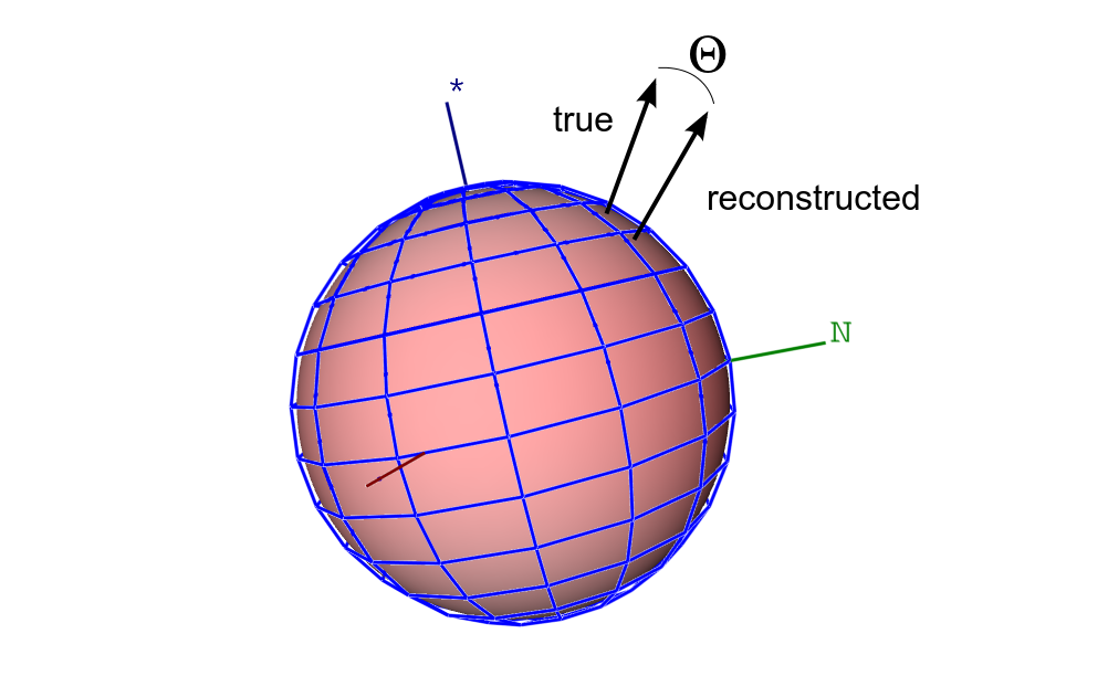
Figure 3: The angular deviation is the deviation $\Theta$ between the reconstructed direction of the lepton, in the canonical coordinate system defined by the directions $\left\{{-\vec{T}},{\vec{N}},{\vec{q}}\right\}$, and the true direction.

As we will prove below, all of the above detector effects are incorporated analytically by replacing the coefficients $a_{l,m}(\vec{\alpha})$ by new coefficients ${\cal A}_{l,m}(\vec{\alpha})$ according to

$$a_{l,m}(\vec{\alpha})\rightarrow{\cal A}_{l,m}(\vec{\alpha})\equiv f_{s}{\frac{2}{2l+1}}\frac{G_{\lambda,\lambda^{\prime},l}^{\mu,\mu^{\prime},m}a_{\lambda,\mu}(\vec{\alpha})e_{\lambda^{\prime},\mu^{\prime}}r_{l}}{(-1)^{\sigma}a_{\kappa,\sigma}(\vec{\alpha}){e_{\kappa,-\sigma}}}+(1-f_{s})b_{l,m}\,.$$ (19)

In this expression $G_{\lambda,\lambda^{\prime},l}^{\mu,\mu^{\prime},m}$ is the Gaunt coefficient, related to the Clebsh-Gordan coefficients $C^{\mu,\mu^{\prime},m}_{\lambda,\lambda^{\prime},l}$ by the equation:

$$G_{\lambda,\lambda^{\prime},l}^{\mu,\mu^{\prime},m}=\sqrt{\frac{(2\lambda+1)(2\lambda^{\prime}+1)}{4\pi(2l+1)}}C^{0,0,0}_{\lambda\lambda^{\prime}l}C^{\mu,\mu^{\prime},m}_{\lambda,\lambda^{\prime},l}\,.$$ (20)

Proof Start with the “raw physics” coefficients $a_{l,m}$ given in eq. 15. First we will add detector efficiency effects, then we will add resolution effects, and finally we will add the background. Denote the PDF before these effects as

$$\rho_{p}(\theta^{*},\phi^{*};\vec{\alpha})=a_{l,m}(\vec{\alpha})Y_{l}^{m}(\theta^{*},\phi^{*}).$$ (21)

To include detector efficiency, we multiply by the efficiency function $\epsilon(\theta^{*},\phi^{*};\vec{\alpha})$ and normalize again

$$\rho_{e}(\theta^{*},\phi^{*};\vec{\alpha}) = N\cdot\epsilon(\theta^{*},\phi^{*};\vec{\alpha})\rho_{p}(\theta^{*},\phi^{*};\vec{\alpha})$$ (22)

$$= N\cdot e_{l^{\prime},m^{\prime}}Y_{l^{\prime},m^{\prime}}(\theta^{*},\phi^{*})a_{l,m}(\vec{\alpha})Y_{l}^{m}(\theta^{*},\phi^{*})$$

where $N$ is a normalization constant defined as

$$1/N = \int_{4\pi}\rho_{p}(\theta^{*},\phi^{*})\epsilon(\theta^{*},\phi^{*})d\Omega$$ (23)

$$= \int_{4\pi}e_{l^{\prime},m^{\prime}}Y_{l^{\prime}}^{m^{\prime}}(\theta^{*},\phi^{*})a_{l,m}(\vec{\alpha})Y_{l}^{m}(\theta^{*},\phi^{*})d\Omega$$

$$= (-1)^{m^{\prime}}a_{l,m}(\vec{\alpha})e_{l^{\prime},m^{\prime}}\int_{4\pi}Y_{l}^{m}(\theta^{*},\phi^{*})Y_{l^{\prime}}^{-m^{\prime}*}(\theta^{*},\phi^{*})d\Omega$$

$$= (-1)^{m^{\prime}}a_{l,m}(\vec{\alpha})e_{l^{\prime},m^{\prime}}\delta_{l,l^{\prime}}\delta_{m,-m^{\prime}}$$

$$= (-1)^{m}a_{l,m}(\vec{\alpha})e_{l,-m}$$

so that

$$\rho_{e}(\theta^{*},\phi^{*};\vec{\alpha}) = N\cdot\epsilon(\theta^{*},\phi^{*})\rho_{e}(\theta^{*},\phi^{*};\vec{\alpha})$$ (24)

$$= \frac{e_{l^{\prime},m^{\prime}}Y_{l^{\prime},m^{\prime}}(\theta^{*},\phi^{*})a_{l,m}(\vec{\alpha})Y_{l}^{m}(\theta^{*},\phi^{*})}{(-1)^{m}a_{l,m}(\vec{\alpha})e_{l,-m}}$$

$$= \frac{a_{l,m}(\vec{\alpha})Y_{l}^{m}(\theta^{*},\phi^{*})e_{l^{\prime},m^{\prime}}Y_{l^{\prime}}^{m^{\prime}}(\theta^{*},\phi^{*})}{(-1)^{\sigma}a_{\kappa,\sigma}(\vec{\alpha})e_{\kappa,-\sigma}}$$

$$= \frac{G_{l,l^{\prime},L}^{m,m^{\prime},M}a_{l,m}(\vec{\alpha})e_{l^{\prime},m^{\prime}}Y_{L}^{M}(\theta^{*},\phi^{*})}{(-1)^{\sigma}a_{\kappa,\sigma}(\vec{\alpha})e_{\kappa,-\sigma}}$$

$$= c_{L,M}(\vec{\alpha})Y_{L}^{M}(\theta^{*},\phi^{*})\,,$$

where the coefficients $c_{l,m}$ are

$$c_{l,m}(\vec{\alpha})=\frac{G_{\lambda,\lambda^{\prime},l}^{\mu,\mu^{\prime},m}a_{\lambda,\mu}(\vec{\alpha})e_{\lambda^{\prime},\mu^{\prime}}}{(-1)^{\sigma}a_{\kappa,\sigma}(\vec{\alpha}){e_{\kappa,-\sigma}}}\,.$$ (25)

Here we have used Gaunt’s theoremref:Gaunt for the product of two spherical harmonics,

$$Y_{\lambda}^{\mu}(\theta^{*},\phi^{*})Y_{\lambda^{\prime}}^{\mu^{\prime}}(\theta^{*},\phi^{*})=G_{\lambda,\lambda^{\prime},l}^{\mu,\mu^{\prime},m}Y_{l}^{m}(\theta^{*},\phi^{*})\,.$$ (26)

Thus far we have a normalized PDF for the signal including detector efficiency which is in the same form as the original PDF and represented by the coefficients $c_{l,m}$ given by eq. 25. We are now going to add the detector smearing to that by convolving the signal PDF

$$\rho_{e}(\theta^{*},\phi^{*};\vec{\alpha})=c_{l,m}(\vec{\alpha})Y_{l}^{m}(\theta^{*},\phi^{*})$$ (27)

with the convolution kernel, a linear combination of $M+1$ Legendre polynomials:

$${\cal R}(\Theta)=\sum_{l=0}^{M}r_{l}P_{l}(\cos{\Theta}).$$ (28)

To do this we use an analogue of the convolution theorem. Imagine that $f$ and $g$ are simple functions of one variable. The Fourier transform of the convolution $f*g$ is the product of the Fourier transforms of $f$ and $g$. In spherical polar coordinates the analogous theorem is the Funk-Hecke theorem. It is ideally suited to our needs, because we have been dealing all along with coefficients of an expansion in spherical harmonics. The theorem states ref:funkHecke ; ref:Groemer that

$$\rho_{e}(\theta^{*},\phi^{*};\vec{\alpha})*{\cal R}(\cos{\Theta}) = \sum_{n}^{M}\sum_{m=-n}^{n}\frac{2}{2n+1}r_{n}c_{n,m}(\vec{\alpha})Y_{n}^{m}(\theta^{*},\phi^{*})$$ (29)

$$= d_{l,m}(\vec{\alpha})Y_{l}^{m}(\theta^{*},\phi^{*})$$

where

$$d_{l,m}(\vec{\alpha}) \equiv {\frac{2}{2l+1}}r_{l}c_{l,m}(\vec{\alpha})$$ (30)

$$= {\frac{2}{2l+1}}\frac{G_{\lambda,\lambda^{\prime},l}^{\mu,\mu^{\prime},m}a_{\lambda\mu}(\vec{\alpha})e_{\lambda^{\prime}\mu^{\prime}}r_{l}}{(-1)^{\sigma}a_{\kappa,\sigma}(\vec{\alpha}){e_{\kappa,-\sigma}}}$$

(no summation over l) which vanish for $l>M$.

Finally, we add the background by taking a simple linear combination of the the coefficients. The coefficients for the full PDF including efficiency, resolution, and background are therefore:

$${\cal A}_{l,m}(\vec{\alpha})=f_{s}{\frac{2}{2l+1}}\frac{G_{\lambda,\lambda^{\prime},l}^{\mu,\mu^{\prime},m}a_{\lambda,\mu}(\vec{\alpha})e_{\lambda^{\prime},\mu^{\prime}}r_{l}}{(-1)^{\sigma}a_{\kappa,\sigma}(\vec{\alpha}){e_{\kappa,-\sigma}}}+(1-f_{s})b_{l,m}\,.$$ (31)

There is no summation over $l$ in this formula.

4.1 Background

In this section we outline a method to obtain the expansion coefficients $b_{l,m}$ of an angular decomposition of the background function $\beta(\theta^{*},\phi^{*})$. The input to the method is a dataset ${\cal B}=\left\{(\theta^{*}_{0},\phi^{*}_{0}),(\theta^{*}_{1},\phi^{*}_{1})...(\theta^{*}_{n-1},\phi^{*}_{n-1})\right\}$ of synthetic data from simulation, real data from a control sample, or a mix. For example, it could consist of simulated background events which have been subject to the same reconstruction procedures as actual collider data. The background coefficients can be obtained by fitting this dataset. Two steps are required.

First, a parametrized, real, positive-definite background function is constructed:

$$\beta(\theta^{*},\phi^{*})=\left|\sum_{l,m}g_{l,m}Y_{l}^{m}(\theta^{*},\phi^{*})\right|^{2}$$ (32)

where the $g_{l,m}$ are coefficients satisfying

$$\sum_{l,m}|g_{l,m}|^{2}=1\,.$$ (33)

The constants $g_{l,m}$ can be determined in a likelihood fit to the dataset ${\cal B}$. Then, the $b_{l,m}$ are obtained from the $g_{l,m}$ in the following way. First, write

$$\beta(\theta^{*},\phi^{*}) = g_{l,m}g^{*}_{l^{\prime},m^{\prime}}Y_{l}^{m}(\theta^{*},\phi^{*})Y_{l^{\prime}}^{m^{\prime}*}(\theta^{*},\phi^{*})$$ (34)

$$= g_{l,m}g^{*}_{l^{\prime},m^{\prime}}(-1)^{m^{\prime}}Y_{l}^{m}(\theta^{*},\phi^{*})Y_{l^{\prime}}^{-m^{\prime}}(\theta^{*},\phi^{*})$$

$$= g_{l,m}g^{*}_{l^{\prime},m^{\prime}}(-1)^{m^{\prime}}G_{l,l^{\prime},L}^{m,-m^{\prime},M}Y_{L}^{M}(\theta^{*},\phi^{*})$$

so that the translation from the $g_{l,m}$ to the $b_{l,m}$ is via the relation:

$$b_{L,M}=g_{l,m}g^{*}_{l^{\prime},m^{\prime}}(-1)^{m^{\prime}}\sqrt{\frac{(2l+1)(2l^{\prime}+1)}{4\pi(2L+1)}}C^{0,0,0}_{l,l^{\prime},L}C^{m,-m^{\prime},M}_{l,l^{\prime},L}$$ (35)

where we have expressed the Gaunt coefficients in terms of the Clebsh-Gordan coefficients using eq. 20. To summarize, we first devise a function which is by construction a real-valued positive definite function to describe the background. We then fit that function to the background dataset ${\cal B}$ to obtain the background coefficients, which can then be translated into a more convenient form using eq. 35. The fit for $g_{l,m}$ is based on a likelihood function

$${\cal L}(g_{l,m})=\beta({\cal B};{g_{l,m}})=\prod_{i=0}^{n-1}\beta(\theta^{*}_{i},\phi^{*}_{i};g_{l,m})\,.$$ (36)

The quantity

$$-2\ln{\cal L}(g_{l,m}) = -2\sum_{i=0}^{n-1}\ln{\beta(\theta^{*}_{i},\phi^{*}_{i};g_{l,m})}$$ (37)

$$= -2\sum_{i=0}^{n-1}\ln|g_{l,m}\cdot y^{i}_{l,m}|^{2}\,,$$

where $y^{i}_{l,m}\equiv Y_{l}^{m}(\theta^{*}_{i},\phi^{*}_{i})$, is computed and minimized over all of the coefficients $g_{l,m}$. When weighted events are available, the weight $w_{i}$ can be incorporated as a Bayesian prior in the likelihood function, which leads to only a slight modification of the above formula:

$$-2\ln{\cal L}(g_{l,m})=-2\sum_{i=0}^{n-1}w_{i}\ln|g_{l,m}\cdot y^{i}_{l,m}|^{2}\,.$$ (38)

The fits are best carried out using a parametrization of the coefficients in eq. 33 which insures a positive-definite PDF, within rectangular bounds on the parameters. Such a parametrization prevents the fit from straying into physically disallowed portions of the parameter space, where the usual punishment to the user is a negative likelihood function with an undefined logarithm, followed by a core dump during the minimization step.

The phase of the $l=0$ component will be taken to be zero. For each additional set of components $l$, $m=\{-l,-l+1,...l-1,l\}$ we add $2(2l+1)$ additional parameters defined in the following way:

• one fraction

  $$F_{l}\equiv\sum_{i\geq l}^{l_{max}}\sum_{m=-i}^{i}|g_{i,m}|^{2};$$

• one phase $\varphi_{l,0}\equiv\arg{(g_{l,0})}$;

• then, for each $m\in 1,2,...l$

  • one fraction

    $$F_{l,m}\equiv\sum_{i\geq m}^{l}(|g_{l,i}|^{2}+|g_{l,-i}|^{2});$$

  • one fraction

    $$s_{l,m}\equiv\frac{|g_{l,m}|^{2}}{|g_{l,m}|^{2}+|g_{l,-m}|^{2}};$$

  • one phase $\varphi_{l,m}\equiv\arg{(g_{l,m})}$;

  • one phase $\varphi_{l,-m}\equiv\arg{(g_{l,-m})}$.

All of the fractions can vary on the interval [0, 1], while the phases need not be bounded at all. In the appendix we show that this minimization can be carried out analytically for a very fast estimate of the background shape parameters. From the estimated values of the $g_{l,m}$ we obtain the estimated value of the $b_{l,m}$ with the use of eq. 35.

4.2 Efficiency

In this section we outline a method to obtain the expansion coefficients $e_{l,m}$ of an angular decomposition of the efficiency function $\epsilon(\theta^{*},\phi^{*})$. The input to the method is simulated signal events which have been subject to the same reconstruction procedures as actual collider data. The dataset contains not only those events which pass the selection criteria, but also those which fail. The coefficients can be obtained by fitting the simulated data as we outline here. Two steps are required.

First, a parametrized, real, positive-definite efficiency function is constructed:

$$\epsilon(\theta^{*},\phi^{*})=A^{2}\cdot\left|\sum_{l,m}f_{l,m}Y_{l}^{m}(\theta^{*},\phi^{*})\right|^{2}$$ (39)

where the $f_{l,m}$ are coefficients satisfying

$$\sum_{l,m}|f_{l,m}|^{2}=1$$ (40)

and $A$ is an overall efficiency factor. The constants $f_{l,m}$ and the overall efficiency factor $A$ can be determined in a likelihood fit to signal Monte Carlo. Then, the $e_{l,m}$ are obtained from the $f_{l,m}$ through a set of algebraic manipulations that parallel those of eq. 35 in order to obtain:

$$e_{L,M}=A^{2}f_{l,m}f^{*}_{l^{\prime},m^{\prime}}(-1)^{m^{\prime}}\sqrt{\frac{(2l+1)(2l^{\prime}+1)}{4\pi(2L+1)}}C^{0,0,0}_{l,l^{\prime},L}C^{m,-m^{\prime},M}_{l,l^{\prime},L}\,.$$ (41)

Among the quantities recorded for the $i^{th}$ event in a data sample derived from Monte Carlo simulation are the truth values of $\theta^{*}$ and $\phi^{*}$, and a discrete variable $s$ describing whether or not the generated event was accepted by the final analysis cuts. We let $s=1$ indicate that the event was accepted and $s=0$ indicate that it was rejected. The probability for this to happen is

$$P_{i}(s;\theta^{*},\phi^{*},f_{l,m})=\delta_{1s}\epsilon(\theta^{*},\phi^{*};f_{l,m})+\delta_{0s}\left(1-\epsilon(\theta^{*},\phi^{*};f_{l,m})\right)\,.$$ (42)

We can estimate the parameters of the efficiency by minimizing

$$-2\ln{\cal L}(f_{l,m})=-2\sum_{i}\ln{\left(\delta_{1s_{i}}\epsilon(\theta^{*}_{i},\phi^{*}_{i};f_{l,m})+\delta_{0s_{i}}(1-\epsilon(\theta^{*}_{i},\phi^{*}_{i};f_{l,m})\right)}\,.$$ (43)

In case weighted events are used we incorporate the weight $w_{i}$ of the event as

$$-2\ln{\cal L}(f_{l,m})=-2\sum_{i}w_{i}\ln{\left(\delta_{1s_{i}}\epsilon(\theta^{*}_{i},\phi^{*}_{i};f_{l,m})+\delta_{0s_{i}}(1-\epsilon(\theta^{*}_{i},\phi^{*}_{i};f_{l,m})\right)}\,.$$ (44)

The coefficients $f_{l,m}$ and the overall efficiency factor $A$ can parametrized and fit as described in the previous section.

4.3 Angular resolution

In this section we show how to obtain coefficients $r_{l}$ of an expansion of the resolution function ${\cal R}(\Theta)$ in terms of Legendre polynomials:

$${\cal R}(\Theta)=r_{l}P_{l}(\cos{\Theta}).$$ (45)

This model assumes that the probability of a given deviation in measured lepton direction is universal, having no dependence on lepton direction and no anisotropy. Input to the fit is simulated data subject to the same reconstruction procedures as real data. For each event the true and reconstructed lepton directions in $\theta^{*}$, $\phi^{*}$ space are recorded and the angular deviation is computed. The coefficients are obtained by fitting a normalized, positive-definite fitting function to the distribution of angular deviations. The fitting function is

$${\cal R}(\Theta)=\left|u_{l}\sqrt{\frac{2l+1}{2}}\cdot P_{l}(\cos{\Theta})\right|^{2}$$ (46)

where $u_{l}$ are complex coefficients satisfying

$$\sum_{l}|u_{l}|^{2}=1\,.$$ (47)

We parametrize these coefficients along the same lines as in previous sections and then re-express the resolution function ${\cal R}(\Theta)$ as an expansion in Legendre polynomials (rather than the square of such an expansion), using a variant of Gaunt’s theorem:

$${\cal R}(\Theta) = \left|u_{l}\sqrt{\frac{2l+1.0}{2.0}}P_{l}(\cos{\Theta})\right|^{2}$$ (48)

$$= \frac{1}{2}u_{l}u^{*}_{l^{\prime}}\sqrt{(2l+1.0)(2l^{\prime}+1)}P_{l}(\cos{\Theta})P_{l^{\prime}}(\cos{\Theta})$$

$$= \sqrt{(2L+1)\pi}u_{l}u^{*}_{l^{\prime}}G_{l,l^{\prime},L}^{0,0,0}P_{L}(\cos{\Theta})$$

which has the form:

$${\cal R}(\Theta)=r_{L}P_{L}(\cos{\Theta}),$$ (49)

the $r_{L}$ being given by:

$$r_{L}=u_{l}u^{*}_{l^{\prime}}\sqrt{\frac{(2l+1)(2l^{\prime}+1)}{4}}\left[C^{0,0,0}_{l,l^{\prime},L}\right]^{2}$$ (50)

using again a Gaunt expansion for the product of two Legendre polynomials, expressed in terms of Clebsh-Gordan coefficients. Again, we use the now-familiar strategy to fit a positive-definite, normalized function to our simulated data, and then (this time with eq. 50) transform to a more convenient form that can be used in eq. 19.

5 Fit strategies

The fractions $F_{0}$ of longitudinal $W$ bosons, $F_{+}$ of right-handed $W$ bosons, and $F_{-}$ of left-handed $W$ bosons are commonly encountered in the literature on top quark couplings ref:Kane . The relationship between these helicity fractions and our parametrization is:

$$f_{1} = F_{+}+F_{-}=1-F_{0}$$

$$f_{1}^{+} = F_{+}/(F_{+}+F_{-})\,.$$ (51)

SM values for the helicity fractions computed to next-to-next-to-leading order are ref:theoryHelicity :

$$F_{+} = (1.7\pm 0.1)\times 10^{-3}$$

$$F_{0} = 0.687\pm 0.005$$

$$F_{-} = 0.311\pm 0.005\$$ (52)

implying:

$$f_{1} =F_{+}+F_{-}=1-F_{0}=0.313\pm 0.005$$

$$f_{1}^{+} =F_{+}/(F_{+}+F_{-})=.00543\pm 0.00033$$ (53)

while also in the SM we expect

$$f_{0}^{+}={\cal O}\left(\frac{m_{b}^{2}}{m_{W}^{2}}\right)\,.$$ (54)

These values have important consequences for strategies to extract these parameters from a dataset using likelihood techniques. First, they imply that at the SM point, $A_{1,1/2}$ and $A_{0,1/2}$ are both nearly zero. The fractions are practically on the edge of the physical parameter space, and the likelihood becomes invariant to the parameter $\delta_{+}$. Under these circumstances the double differential decay rate, eq. 6, loses its sensitivity to the polarization $P$ and the parameter $f_{0}^{+}$ separately, and instead depends only on the product $P\sqrt{1-f_{0}^{+}}$. Since no other measurement presently determines $f_{0}^{+}$, we appear to be insensitive to a valuable piece of information near to the SM expected point.

On the other hand we are still very sensitive to the most important physics parameter, $\delta_{-}$, because the $P\sqrt{1-f_{0}^{+}}$ will now appear as the amplitude in the $\phi^{*}$-modulation, where $\delta_{-}$ plays the role of a phase. To leading order in the anomalous couplings,

$$\delta_{-}=-\tan^{-1}\left[(x_{W}^{-1}-x_{W}){\rm Im}(g_{R})\right]$$ (55)

where $x_{W}=m_{W}/m_{t}$. Thus we can get a clean measurement of the most important physics quantity in the analysis, with no external dependence on the single top quark polarization.

Helicity fractions in top quark decay have been measured in $t{\bar{t}}$ production by CDF(ref:cdfWHel1 -ref:cdfWHel8 ) and by DØ (ref:d0WHel1 -ref:d0WHel5 ) and combined ref:comboWHel ; and more recently by ATLAS ref:atlasWHel and CMS (ref:cmsWHel ,ref:cmsWHelSingle ). Parameters extracted from single top quark $t$-channel events using techniques based upon the likelihood function described here can be compared results from the $t{\bar{t}}$ analysis; consistency between the two measured values could provide strong indications that the background is well understood and the signal is consistent with single top quark production. Once the consistency was established, the measurements could be imported into the likelihood as an external constraint.

6 Extended models of detector effects

The treatment of detector effects developed in the previous sections is based on a model of detector effects that may, when used with real data, prove too simple to describe all effects. Namely, the model assumes that detector smearing is isotropic and does not depend on angle, and it also assumes that the efficiency function does not depend upon the physics parameters. In this section we show how these effects can be properly handled within the same framework of orthogonal polynomials, at the price of a small increase in the complexity of the formulation.

6.1 Extended models of angular resolution

Let the true direction of a lepton in $\theta^{*}$, $\phi^{*}$ space be denoted by

$${\hat{u}}\equiv(\sin\theta_{T}^{*}\cos\phi^{*}_{T},\sin\theta_{T}^{*}\sin\phi_{T}^{*},\cos\theta_{T}^{*})$$ (56)

and the reconstructed direction by

$${\hat{v}}\equiv(\sin\theta^{*}\cos\phi^{*},\sin\theta^{*}\sin\phi^{*},\cos\theta^{*})\,.$$ (57)

As usual we express the underlying probability density as $f(\hat{u})=a_{l,m}Y_{l}^{m}(\theta^{*}_{T},\phi^{*}_{T})$. The probability that a lepton produced along ${\hat{u}}$ will be reconstructed at $\hat{v}$ will be denoted as $g(\hat{u},\hat{v})$. The observed distribution $h(\hat{v})$ is then the integral

$$h(\hat{v})=\int f(\hat{u})g(\hat{u},\hat{v})d\Omega^{*}_{T}\,.$$ (58)

The assumption of isotropic, angle-independent smearing is equivalent to the condition that

$$g(\hat{u},\hat{v})=g({\hat{u}}\cdot{\hat{v}})\,,$$ (59)

i.e. that the smearing probability only depends upon the angle between true and reconstructed directions. Under these circumstances, one can expand

$$g({\hat{u}}\cdot{\hat{v}})=\frac{1}{2\pi}r_{k}P_{k}(\hat{u}\cdot\hat{v})$$ (60)

and write

$$h(\hat{v})=\frac{1}{2\pi}a_{l,m}r_{k}\int Y_{l}^{m}(\theta^{*}_{T},\phi^{*}_{T})P_{k}(\hat{u}\cdot\hat{v})d\Omega^{*}_{T}\,.$$ (61)

Using the addition theorem,

$$P_{k}(\hat{u}\cdot\hat{v})=\frac{4\pi}{2k+1}\sum_{n=-k}^{k}Y_{k}^{n*}(\theta^{*}_{T},\phi^{*}_{T})Y_{k}^{n}(\theta^{*},\phi^{*})$$ (62)

(no summation over $k$ on the right hand side), we have

$$h(\hat{v}) = \frac{2}{2k+1}a_{l,m}r_{k}\int Y_{l}^{m}(\theta^{*}_{T},\phi^{*}_{T})Y_{k}^{n*}(\theta^{*}_{T},\phi^{*}_{T})Y_{k}^{n}(\theta^{*},\phi^{*})d\Omega^{*}_{T}$$ (63)

$$= \frac{2}{2k+1}a_{l,m}r_{k}\delta_{l,k}\delta_{m,n}Y_{k}^{n}(\theta^{*},\phi^{*})$$

$$= d_{l,m}Y_{l}^{m}(\theta^{*},\phi^{*})$$

where

$$d_{l,m}=\frac{2}{2l+1}a_{l,m}r_{l}$$ (64)

(no summation over l) and one recovers the Funk-Hecke theorem, eqs. 29 and 30. Now, if

$$g(\hat{u},\hat{v})\neq g({\hat{u}}\cdot{\hat{v}})$$ (65)

then we can still expand the resolution function as

$$g(\hat{u},\hat{v})=r_{l,m,l^{\prime},m^{\prime}}Y_{l}^{m}(\theta^{*}_{T},\phi^{*}_{T})Y_{l^{\prime}}^{m^{\prime}}(\theta^{*},\phi^{*})\,,$$ (66)

in which case a few algebraic manipulations give us

$$h(\hat{v})=a_{l,-m}r_{l,m,l^{\prime},m^{\prime}}(-1)^{m}Y_{l^{\prime}}^{m^{\prime}}(\theta^{*},\phi^{*})$$ (67)

which is another type of convolution theorem for spherical harmonics, but with a completely general convolution kernel. Using this instead of the Funk-Hecke theorem modifies the coefficient formula, eq. 31, so that it instead reads:

$${\cal A}_{l,m}(\vec{\alpha})=\frac{G_{\lambda,\lambda^{\prime},l^{\prime}}^{\mu,\mu^{\prime},-m^{\prime}}a_{\lambda\mu}(\vec{\alpha})e_{\lambda^{\prime}\mu^{\prime}}r_{l^{\prime},m^{\prime},l,m}(-1)^{m^{\prime}}}{(-1)^{\sigma}a_{\kappa,\sigma}(\vec{\alpha}){e_{\kappa,-\sigma}}}+(1-f_{s})b_{l,m}\,.$$ (68)

To find the coefficients $r_{l,m,l^{\prime},m^{\prime}}$ we construct a positive-definite normalized fitting function:

$$g(\hat{u},\hat{v})={\cal R}(\theta^{*}_{T},\phi^{*}_{T},\theta^{*},\phi^{*})=\left|\sum_{\lambda,\mu,\kappa,\nu}s_{\lambda,\mu,\kappa,\nu}Y_{\lambda}^{\mu}(\theta^{*}_{T},\phi^{*}_{T})Y_{\kappa}^{\nu}(\theta^{*},\phi^{*})\right|^{2}$$ (69)

where the $s_{\lambda,\mu,\kappa,\nu}$ are complex coefficients satisfying

$$\sum_{\lambda,\mu,\kappa,\nu}|s_{\lambda,\mu,\kappa,\nu}|^{2}=1\,.$$ (70)

The constants $s_{\lambda,\mu,\kappa,\nu}$ can be determined in a likelihood fit to signal Monte Carlo. Then, the $r_{l,m,l^{\prime},m^{\prime}}$ are obtained from the $s_{\lambda,\mu,\kappa,\nu}$ via the relationship

$$r_{l,m,l^{\prime},m^{\prime}} = (-1)^{\mu^{\prime}+\nu^{\prime}}G^{\mu,-\mu^{\prime},m}_{\lambda,\lambda^{\prime},l}G^{\nu,-\nu^{\prime},m^{\prime}}_{\kappa,\kappa^{\prime},l^{\prime}}s_{\lambda,\mu,\kappa,\nu}s^{*}_{\lambda^{\prime},\mu^{\prime},\kappa^{\prime},\nu^{\prime}}\,.$$ (71)

6.2 Variation of the Efficiency

It can happen that the efficiency, $\epsilon(\theta^{*},\phi^{*})=e_{l,m}Y_{l}^{m}(\theta^{*},\phi^{*})$, varies as a function of the physics parameters $\vec{\alpha}$:

$$\epsilon(\theta^{*},\phi^{*};\vec{\alpha})=e_{l,m}(\vec{\alpha})Y_{l}^{m}(\theta^{*},\phi^{*})\,.$$ (72)

This arises because of the integration over the angle $\theta$, which we carried out to obtain eq. 6. The efficiency as a function of three observable angles $\varepsilon(\theta,\theta^{*},\phi^{*})$, when projected into only two angles ($\theta^{*}$ and $\phi^{*}$), acquires a dependence on $\vec{\alpha}$, as follows:

$$\epsilon(\theta^{*},\phi^{*};\vec{\alpha})=\frac{\int\varrho(\theta,\theta^{*},\phi^{*};\vec{\alpha})\varepsilon(\theta,\theta^{*},\phi^{*})d(\cos\theta)}{\int\varrho(\theta,\theta^{*},\phi^{*})d(\cos\theta)}\,.$$ (73)

This dependency can be accounted for with a slight modification of the formalism developed here, without sacrificing any of the mathematical elegance. We can now express the triple differential decay rate, eq. 5 as

$$\varrho(\theta,\theta^{*},\phi^{*})=s_{k,n,l,m}(\vec{\alpha})P_{k}^{n}(\cos\theta)Y_{l}^{m}(\theta^{*},\phi^{*})$$ (74)

where:

$$\begin{split}&s_{0,0,0,0}=\frac{a_{0,0}}{4\pi}\,,\qquad s_{0,0,1,0}=\frac{a_{1,0}}{4\pi}\,,\qquad s_{0,0,2,0}=\frac{a_{2,0}}{4\pi}\,,\qquad s_{1,1,1,-1}=-\pi^{2}a_{1,-1}\,,\\ &s_{1,1,1,1}=-\pi^{2}a_{1,1}\,,\qquad s_{1,1,2,-1}=-\pi^{2}a_{2,-1}\,,\qquad s_{1,1,2,1}=-\pi^{2}a_{2,1}\,,\\ &s_{1,0,0,0}=\frac{P}{(4\pi)^{3/2}}\left(f_{1}\left(2f_{1}^{+}-1\right)-\left(1-f_{1}\right)\left(2f_{0}^{+}-1\right)\right)\,,\qquad s_{1,0,1,0}=\frac{P\sqrt{3}}{2(4\pi)^{3/2}}f_{1}\,,\\ &s_{1,0,2,0}=\frac{P}{\sqrt{5}(4\pi)^{3/2}}\left(\frac{1}{2}f_{1}\left(2f_{1}^{+}-1\right)+\left(1-f_{1}\right)\left(2f_{0}^{+}-1\right)\right)\\ \end{split}$$ (75)

and all of the other coefficients are zero. Expanding the efficiency function,

$$\varepsilon(\theta,\theta^{*},\phi^{*})=w_{k,l,m}P_{k}(\cos\theta)Y_{l}^{m}(\theta^{*},\phi^{*})\,,$$ (76)

and integrating over $\cos\theta$ gives us:

$$\epsilon(\theta^{*},\phi^{*};\vec{\alpha}) = \frac{\int\varrho(\theta,\theta^{*},\phi^{*};\vec{\alpha})\varepsilon(\theta,\theta^{*},\phi^{*})d(\cos\theta)}{\int\varrho(\theta,\theta^{*},\phi^{*})d(\cos\theta)}$$ (77)

$$= \frac{\int s_{\kappa,\nu,\lambda,\mu}(\vec{\alpha})P_{\kappa}^{\nu}(\cos\theta)Y_{\lambda}^{\mu}(\theta^{*},\phi^{*})\cdot w_{k,l,m}P_{k}(\cos\theta)Y_{l}^{m}(\theta^{*},\phi^{*})d(\cos\theta)}{a_{\lambda,\mu}(\vec{\alpha})Y_{\lambda}^{\mu}(\theta^{*},\phi^{*})}$$

$$= \frac{\int s_{\kappa,\nu,\lambda,\mu}(\vec{\alpha})P_{\kappa}^{\nu}(\cos\theta)Y_{\lambda}^{\mu}(\theta^{*},\phi^{*})\cdot w_{k,l,m}P_{k}(\cos\theta)Y_{l}^{m}(\theta^{*},\phi^{*})d(\cos\theta)}{a_{\lambda,\mu}(\vec{\alpha})Y_{\lambda}^{\mu}(\theta^{*},\phi^{*})}$$

$$= \frac{s_{\kappa,\nu,\lambda,\mu}(\vec{\alpha})w_{k,l,m}Y_{\lambda}^{\mu}(\theta^{*},\phi^{*})Y_{l}^{m}(\theta^{*},\phi^{*})}{a_{\lambda,\mu}(\vec{\alpha})Y_{\lambda}^{\mu}(\theta^{*},\phi^{*})}\int P_{k}(\cos\theta)P_{\kappa}^{\nu}(\cos\theta)d(\cos\theta)$$

$$= \frac{S_{k,\kappa}^{\nu}s_{\kappa,\nu,\lambda,\mu}(\vec{\alpha})w_{k,l,m}Y_{\lambda}^{\mu}(\theta^{*},\phi^{*})Y_{l}^{m}(\theta^{*},\phi^{*})}{a_{\lambda,\mu}(\vec{\alpha})Y_{\lambda}^{\mu}(\theta^{*},\phi^{*})}$$

$$= \frac{G_{\lambda,l,L}^{\mu,m,M}S_{k,\kappa}^{\nu}s_{\kappa,\nu,\lambda,\mu}(\vec{\alpha})w_{k,l,m}Y_{L}^{M}(\theta^{*},\phi^{*})}{a_{\lambda,\mu}(\vec{\alpha})Y_{\lambda}^{\mu}(\theta^{*},\phi^{*})}\,,$$

where we have introduced the constant

$$S_{k,\kappa}^{\nu}\equiv\int_{-1}^{1}P_{k}(x)P_{\kappa}^{\nu}(x)dx$$ (78)

An analytic expression for this integral can be easily derived with the use of Gaunt’s theorem:

$$S_{k,\kappa}^{\nu}=\sqrt{\frac{4\pi(2L+1)}{(2k+1)(2\kappa+1)}\frac{(\kappa+\nu)!}{(\kappa-\nu)!}\frac{(L-\nu)!}{(L+\nu)!}}G^{0,\nu,\nu}_{k,\kappa,L}R_{L}^{M}$$ (79)

where

$$R_{L}^{M}\equiv\int_{-1}^{1}P_{L}^{M}(x)dx$$ (80)

is the integral of the associated Legendre function. Explicit expressions for this integral can be found in ref. ref:AssInt . Our goal here is to obtain an expression for the coefficients $e_{L,M}(\vec{\alpha})$; we can achieve this by equating expansion 77 to the expansion  72:

$$\epsilon(\theta^{*},\phi^{*};\vec{\alpha}) = \frac{G_{\lambda,l,L}^{\mu,m,M}S_{k,\kappa}^{\nu}s_{\kappa,\nu,\lambda,\mu}(\vec{\alpha})w_{k,l,m}Y_{L}^{M}(\theta^{*},\phi^{*})}{a_{\lambda,\mu}(\vec{\alpha})Y_{\lambda}^{\mu}(\theta^{*},\phi^{*})}$$ (81)

$$= e_{l,m}(\vec{\alpha})Y_{l}^{m}(\theta^{*},\phi^{*})$$

so

$${G_{\lambda,l,L}^{\mu,m,M}S_{k,\kappa}^{\nu}s_{\kappa,\nu,\lambda,\mu}(\vec{\alpha})w_{k,l,m}Y_{L}^{M}(\theta^{*},\phi^{*})} = {a_{\lambda,\mu}(\vec{\alpha})e_{l,m}(\vec{\alpha})Y_{\lambda}^{\mu}(\theta^{*},\phi^{*})}Y_{l}^{m}(\theta^{*},\phi^{*})$$ (82)

$$= {a_{\lambda,\mu}(\vec{\alpha})e_{l,m}(\vec{\alpha})G_{\lambda,l,L}^{\mu,m,M}Y_{L}^{M}(\theta^{*},\phi^{*})}$$

from which we can conclude that:

$$S_{k,\kappa}^{\nu}w_{k,l,m}s_{\kappa,\nu,\lambda,\mu}(\vec{\alpha}) = {a_{\lambda,\mu}(\vec{\alpha})e_{l,m}(\vec{\alpha})}\,,$$ (83)

or

$$e_{l,m}(\vec{\alpha}) = \frac{S_{k,\kappa}^{\nu}w_{k,l,m}s_{\kappa,\nu,\lambda,\mu}(\vec{\alpha})}{a_{\lambda,\mu}(\vec{\alpha})}\,.$$ (84)

This expression now contains the variation of the efficiency parameters as a function of physics parameters $\vec{\alpha}$. Eq. 19 can now be used without modification, provided that the coefficients in eq. 84 are taken instead of fixed coefficients.

This leaves us with the problem of determining the coefficients $w_{k,l,m}$. This can be carried out in a straightforward extension of the methods previously discussed. First, we construct a parametrized efficiency function which is positive-definite:

$$\epsilon\left(\theta^{\ast},\varphi^{\ast},\theta\right)=A^{2}\cdot\left|\sum_{k,l,m}t_{k,l,m}P_{k}(\cos\theta)Y_{l}^{m}(\theta^{\ast},\varphi^{\ast})\right|^{2}$$ (85)

where the $t_{k,l,m}$ are complex coefficients satisfying

$$\sum_{k,l,m}|t_{k,l,m}|^{2}=1\,.$$ (86)

The coefficients $t_{k,l,m}$ can be determined from a likelihood fit to signal Monte Carlo. Then we write

$$\epsilon(\theta^{*},\varphi^{*},\theta)=A^{2}\cdot t_{k,l,m}P_{k}Y_{l}^{m}t_{k^{\prime},l^{\prime},m^{\prime}}^{*}P^{*}_{k^{\prime}}Y_{l^{\prime}}^{-m^{\prime}}(-1)^{m^{\prime}}\,.$$ (87)

Applying Gaunt’s theorem

$$P_{n}(x)P_{n^{\prime}}(x)=\sum_{m=0}^{n+n^{\prime}}G_{m}^{n,n^{\prime}}P_{m}(x)\,,$$ (88)

$$Y_{l}^{m}(\theta,\varphi)Y_{l^{\prime}}^{m^{\prime}}(\theta,\varphi)=\sum_{L,M}G_{l,l^{\prime},L}^{m,m^{\prime},M}Y_{L}^{M}\left(\theta,\varphi\right)\,,$$ (89)

where

$$G_{m}^{n,n^{\prime}}=\left[C_{n,n^{\prime},m}^{0,0,0}\right]^{2}$$ (90)

gives us

$$\epsilon(\theta^{*},\varphi^{*},\theta) = A^{2}\cdot t_{k,l,m}t_{k^{\prime},l^{\prime},m^{\prime}}^{*}G_{i}^{k,k^{\prime}}P_{i}(\cos\theta)G_{l,l^{\prime},L}^{m,{-m^{\prime}},M}Y_{L}^{M}\left(-1\right)^{m^{\prime}}$$ (91)

$$= A^{2}\cdot(-1)^{m^{\prime}}t_{k,l,m}t{{}_{k^{\prime},l^{\prime},m^{\prime}}^{*}}G_{i}^{k,k^{\prime}}G_{l,l^{\prime},L}^{m,{-m^{\prime}},M}P_{i}(\cos\theta)Y_{L}^{M}(\theta^{*},\varphi^{*})\,,$$

so that the translation from the $t_{k,l,m}$ to the $w_{k,l,m}$ is via the relation:

$$w_{i,L,M}=A^{2}\cdot(-1)^{m^{\prime}}t_{k,l,m}t^{*}_{k^{\prime},l^{\prime},m^{\prime}}G_{i}^{k,k^{\prime}}G_{l,l^{\prime},L}^{m,{-m^{\prime}},M}\,.$$ (92)

7 Conclusions

We have presented here formulae for the analysis of the decay of polarized single top quarks produced in the $t$-channel. The formulae can be used in a variety of likelihood-based techniques to precisely measure the $Wtb$ vertex from angular distributions measured at the LHC. While formulae governing the raw physics PDFs are easy to obtain, the main difficulty arises in the convolution of detector effects. In the past only Monte Carlo simulation has been capable of addressing this aspect, and full simulation is too time consuming to be used at each step in a likelihood fit by many orders of magnitude.

A theorem called the Funk-Hecke theorem, related to the convolution theorem but applicable to an angular analysis in spherical harmonics rather than a Fourier transform, is the basis of a practical scheme for convolving detector effects with physics distributions. This scheme, which we outline in this paper, requires Monte Carlo for a description of resolution and efficiency, then uses the formula 19 or simple extensions to carry out the convolution.

We have applied this to the double-differential decay rate in $t$-channel single top quark decay, described by eq. 6. This is made possible by the existence of an angular decomposition of the differential decay rate on one hand, and the properties of orthogonal polynomials on the other. Because these properties can be discovered in many interesting systems, it is likely, that the basic technique can be applied elsewhere. The most interesting systems are those where significant measurement errors are present, coming from the presence of such objects as jets or a neutrino in the final state.

Appendix A Analytic minimization

In this appendix we show that we can analytically minimize the likelihood function for several of our fits when the PDF is expressed in terms of spherical harmonics — this is the way, for example, that track fits are normally carried out in a reconstruction program. Since the computations are long we will illustrate this only for the simplest type of fit, namely the kind we use for the background shape, where the likelihood function is:

$$-2ln\mathcal{L}=\sum_{j}w_{j}\ln(|g_{l,m}y_{l,m}^{j}|^{2})$$ (93)

where the $g_{l,m}$ are complex coefficients. We decompose these into real and imaginary parts

$$g_{l,m}=a_{l,m}+ib_{l,m}$$ (94)

and there are two real parameters for every complex coefficient. Minimizing with respect to the real part $a_{l,m}$ of the coefficients gives us

$$\frac{\partial(-2\ln{\cal L})}{\partial a_{L,M}} = -2\sum_{j}\frac{w_{j}}{|g_{r,s}y_{r,s}^{j}|^{2}}\frac{\partial}{\partial a_{L,M}}\left(|g_{l,m}y_{l,m}^{j}|^{2}\right)\,.$$ (95)

After some straightforward calculation we obtain:

$$\frac{\partial(-2\ln{\cal L})}{\partial a_{L,M}} = -4{\rm Re}\left[\sum_{j}w_{j}\frac{y_{L,M}^{j}}{g_{l,m}y_{l,m}^{j}}\right]\,,$$

$$\frac{\partial(-2\ln{\cal L})}{\partial b_{L,M}} = 4{\rm Im}\left[\sum_{j}w_{j}\frac{y_{L,M}^{j}}{g_{l,m}y_{l,m}^{j}}\right]\,.$$ (96)

Next, we require second derivatives, in particular we need the full $(L_{max}+1)^{2}\times(L_{max}+1)^{2}$ matrix:

$$\left(\begin{array}[]{cc}\frac{\partial^{2}(-2\ln{\cal L})}{\partial a_{\lambda,\mu}\partial a_{L,M}}&\frac{\partial^{2}(-2\ln{\cal L})}{\partial a_{\lambda,\mu}\partial b_{L,M}}\\ \frac{\partial^{2}(-2\ln{\cal L})}{\partial b_{\lambda,\mu}\partial a_{L,M}}&\frac{\partial^{2}(-2\ln{\cal L})}{\partial b_{\lambda,\mu}\partial b_{L,M}}\end{array}\right),$$

which is

$$\frac{\partial^{2}(-2\ln{\cal L})}{\partial a_{R,S}\partial a_{L,M}} = \frac{\partial}{\partial a_{R,S}}\left(-2\sum_{j}w_{j}\left[\frac{y_{L,M}^{j}}{g_{l,m}y_{l,m}^{j}}+CC\right]\right)$$ (97)

$$= +4{\rm Re}\sum_{j}w_{j}\left[\frac{y_{L,M}^{j}y_{R,S}^{j}}{(g_{l,m}y_{l,m}^{j})^{2}}\right]\,.$$

Likewise,

$$\frac{\partial^{2}(-2\ln{\cal L})}{\partial b_{R,S}\partial a_{L,M}} = \frac{\partial}{\partial b_{R,S}}\left(-2\sum_{j}w_{j}\left[\frac{y_{L,M}^{j}}{g_{l,m}y_{l,m}^{j}}+CC\right]\right)$$ (98)

$$= -4{\rm Im}\sum_{j}w_{j}\left[\frac{y_{L,M}^{j}y_{R,S}^{j}}{(g_{l,m}y_{l,m}^{j})^{2}}\right]\,.$$

and

$$\frac{\partial^{2}(-2\ln{\cal L})}{\partial b_{R,S}\partial b_{L,M}} = \frac{\partial}{\partial b_{R,S}}\left(-2\sum_{j}w_{j}\left[i\frac{y_{L,M}^{j}}{g_{l,m}y_{l,m}^{j}}+CC\right]\right)$$ (99)

$$= -4{\rm Re}\sum_{j}w_{j}\left[\frac{y_{L,M}^{j}y_{R,S}^{j}}{(g_{l,m}y_{l,m}^{j})^{2}}\right]\,.$$

To minimize the likelihood, one first assigns random values to the coupling $g_{l,m}.$ Then, one computes the sums

$$S_{1}=\sum_{j}w_{j}\frac{y_{L,M}^{j}}{g_{l,m}y_{l,m}^{j}}\qquad S_{2}=\sum_{j}w_{j}\left[\frac{y_{L,M}^{j}y_{R,S}^{j}}{(g_{l,m}y_{l,m}^{j})^{2}}\right]\,.$$ (100)

The first of these (real and imaginary parts) is used to compute the first derivative of the likelihood, the second is used to compute its second derivative. Taking the real and imaginary parts of the full coefficient set $\{g_{l,m}\}$ as a large, real-valued vector $\vec{\eta}$ and denoting

$$\frac{\partial(-2\ln{\cal L})}{\partial\vec{\eta}} \equiv \vec{\xi}\,,$$

$$\frac{\partial(-2\ln{\cal L})}{\partial\vec{\eta}\partial\vec{\eta}} \equiv \mathbf{\mathbf{H}}$$ (101)

we have:

$$\mathbf{H}\left(\vec{\eta}_{0}-\vec{\eta}\right)=-\vec{\xi}$$ (102)

which relates the parameters which minimize the likelihood, $\vec{\eta}_{0}$, to starting parameters $\vec{\eta}$ and starting derivatives $\vec{\xi}$. The solution is

$$\vec{\eta}_{0}=\mathbf{H}^{-1}\cdot\left(\mathbf{H}\cdot\vec{\eta}-\vec{\xi}\right)\,.$$ (103)

One can test this by computing the derivatives of the likelihood function, $\vec{\xi},$ again at the solution to this equation, as well as the Hessian $\mathbf{H}$; if the first step has not succeeded in locating bringing the fit to a true minimum (because eq. 102 ignores higher order terms) the procedure can be iterated, and when convergence has occurred both the parameter set $\vec{\eta}_{0}$ and the Hessian can be saved, the latter being useful to compute the covariance matrix from the relation $\mathbf{C}^{-1}=\mathbf{H}/2$. For the background fit, some special considerations also apply. First, the likelihood function is insensitive to an overall phase. This degree of freedom can be removed by fixing the phase of $g_{0,0}$ to zero. We also have to deal with the normalization constraint, $g_{l,m}g_{l,m}^{*}=1$. We do this by enlarging the set of parameters with a Lagrange multiplier $\lambda$, and modifying the likelihood correspondingly:

$$-2\ln{\cal L}\rightarrow\Lambda=-2\ln{\cal L}+\lambda(g_{l,m}g_{l,m}^{*}-1)\,.$$ (104)

The extra parameter adds another element to the vector $\vec{\xi}$ which is

$$\frac{\partial\Lambda}{\partial\lambda}=(g_{l,m}g_{l,m}^{*}-1)\,.$$ (105)

The second derivative is zero:

$$\frac{\partial^{2}\Lambda}{\partial\lambda^{2}}=0$$ (106)

but the extra terms modify the derivatives according to

$$\frac{\partial\Lambda}{\partial a_{L,M}} = \frac{\partial\left(-2\ln{\cal L}\right)}{\partial a_{L,M}}+\lambda(g_{L,M}^{*}+g_{L,M})\,,$$

$$\frac{\partial\Lambda}{\partial b_{L,M}} = \frac{\partial\left(-2\ln{\cal L}\right)}{\partial b_{L,M}}+\lambda(ig_{L,M}^{*}-ig_{L,M}),$$ (107)

and the Hessian $\mathbf{H}$ according to

$$\frac{\partial^{2}\Lambda}{\partial a_{R,S}\partial a_{L,M}} = \frac{\partial^{2}\left(-2\ln{\cal L}\right)}{\partial a_{R,S}\partial a_{L,M}}+2\lambda\delta_{R,L}\delta_{S,M}$$

$$\frac{\partial^{2}\Lambda}{\partial b_{R,S}\partial b_{L,M}} = \frac{\partial^{2}\left(-2\ln{\cal L}\right)}{\partial b_{R,S}\partial b_{L,M}}+2\lambda\delta_{R,L}\delta_{S,M}$$

$$\frac{\partial^{2}\Lambda}{\partial b_{R,S}\partial a_{L,M}} = \frac{\partial^{2}\left(-2\ln{\cal L}\right)}{\partial b_{R,S}\partial a_{L,M}}$$

$$\frac{\partial^{2}\Lambda}{\partial\lambda\partial a_{L,M}} = 2{\rm Re}g_{L,M}$$

$$\frac{\partial^{2}\Lambda}{\partial\lambda\partial b_{L,M}} = 2{\rm Im}g_{L,M}$$ (108)

One can now proceed with analytic minimization as in eq. 103 using the enlarged set of parameters and the enlarged Hessian matrix.

References

• (1) CDF and DØ Collaborations, Combination of CDF and DØ results on the mass of the top quark using up to 5.8 fb-1 of data, arXiv:1107.5255
• (2) J.A. Aguilar-Saavedra and J. Bernabéu, $W$ Polarization beyond helicity fractions in top quark decays, Nucl. Phys. B 840 (2010) 349
• (3) G. Feldman and R. Cousins, Unified approach to the classical statistical analysis of small signals, Phys. Rev. D 57 (1998) 3873
• (4) J. Richman, An experimenter’s guide to the helicity formalism, CALT-68-1148 (1984).
• (5) F. James and M. Roos, Minuit: a system for function minimization and analysis of the parameter errors and correlations, Comput. Phys. Commun. 10 (1975) 343
• (6) J.A. Aguilar-Saavedra, A minimal set of top anomalous couplings, Nucl. Phys. B 812 (2009), 181
• (7) J.A. Gaunt, The triplets of helium, Phil. Trans. R. Soc. A 228 (1929) 151
• (8) R. Bari and D. Jacobs, Lambertian reflectance and linear subspaces, IEEE Transactions on Pattern Analysis and Machine Intelligence 25 (2001) 218
• (9) H. Groemer, Geometric applications of Fourier series and spherical harmonics, Cambridge University Press, Cambridge, UK (1996)
• (10) G. Kane, G. Ladinsky, and C. Yuan, Using the top quark for testing standard model and $CP$ predictions, Phys. Rev. D 45 (1992) 124
• (11) A. Czarnecki, J. G. Körner, and J. H. Piclum, Helicity fraction of $W$ bosons from top quark decays at next-to-next-to-leading order in QCD, Phys. Rev. D 81 (2010) 111503
• (12) CDF Collaboration, Measurement of the W boson polarization in top decay at CDF at $\sqrt{s}$ = 1.8 TeV, Phys. Rev. Lett. 84 (2000) 216
• (13) CDF Collaboration, Measurement of the W boson polarization in top decay at CDF at $\sqrt{s}$ = 1.8 TeV, D. E. Acosta et al. (CDF Collaboration) Phys. Rev. D 71 (2005) 031101 [Erratum ibid 71 (2005) 059901]
• (14) CDF Collaboration, Measurement of the helicity of W bosons in top-quark decays , Phys. Rev. D 73 (2006) 111103
• (15) CDF Collaboration, Top quark mass measurement in the lepton plus jets channel using a modified matrix element method, Phys. Rev. Lett. 98 (2007) 072001
• (16) CDF Collaboration, Measurement of the helicity fractions of W bosons from top quark decays using fully reconstructed $t{\bar{t}}$ events with CDF II, Phys. Rev. D 75 (2007) 052001
• (17) CDF Collaboration, Measurement of W-boson helicity fractions in top-quark decays using $\cos\theta^{*}$, Phys. Lett. B 674 (2009) 160
• (18) CDF Collaboration, Measurement of W-boson polarization in top-quark decay in $p{\bar{p}}$ collisions at $\sqrt{s}$ = 1.96 TeV, Phys. Rev. Lett. 105 (2010) 042002
• (19) CDF Collaboration, Measurement of W-boson polarization in top-quark decay using the full CDF run II data set, Phys. Rev. D 87 (2013) 03110
• (20) DØ Collaboration, Search for right-handed W bosons in top quark decay, Phys. Rev. D 72 (2005) 011104
• (21) DØ Collaboration,Helicity of $W$ bosons in lepton + jets $t{\bar{t}}$ events, Phys. Lett. B 617 (2005) 1
• (22) DØ Collaboration,Measurement of the W boson helicity in top quark decays at DØ , Phys. Rev. D 75 (2007) 031102
• (23) DØ Collaboration,Model-independent measurement of the W boson helicity in top quark decays at DØ , Phys. Rev. Lett. 100 (2008) 062004
• (24) DØ Collaboration,Measurement of the W boson helicity in top quark decays using 5.4 fb−1 of $p{\bar{p}}$ collision data, Phys. Rev. D 83 (2011) 032009
• (25) CDF and DØ Collaborations, Combination of CDF and DØ measurements of the $W$ boson helicity in top quark decays, Phys. Rev. D 85 (2012) 071106
• (26) ATLAS Collaboration, Measurement of $W$ boson polarization in top quark decays with the ATLAS detector, JHEP 1206 (2012) 088
• (27) CMS Collaboration, Measurement of W helicity fractions in top pair production with dileptons, CMS-PAS-TOP-11-015
• (28) CMS Collaboration, Measurement of W helicity fractions in single top events topology, CMS-PAS-TOP-11-020
• (29) D. Jepsen, E. Haugh, and J. Hirschfelder,The integral of the associated Legendre function, Proc. Natl. Acad. Sci. U. S. A., 41 645