Isomorphic Strategy Spaces in Game Theory

Copyright ©Michael J. Gagen 2013.

All rights reserved. No part of this book may be reproduced in any form by any electronic or mechanical means (including photocopying, recording, or information storage and retrieval) without permission in writing from the author.

Michael J. Gagen assert his right to be identified as the author of this work.

Preface

This book summarizes ongoing research introducing probability space isomorphic mappings into the strategy spaces of game theory.

This approach is motivated by discrepancies between probability theory and game theory when applied to the same strategic situation. In particular, probability theory and game theory can disagree on calculated values of the Fisher information, the log likelihood function, entropy gradients, the rank and Jacobian of variable transforms, and even the dimensionality and volume of the underlying probability parameter spaces. These differences arise as probability theory employs structure preserving isomorphic mappings when constructing strategy spaces to analyze games. In contrast, game theory uses weaker mappings which change some of the properties of the underlying probability distributions within the mixed strategy space. Here, we explore how using strong isomorphic mappings to define game strategy spaces can alter rational outcomes in simple games .

Specific example games considered are the chain store paradox, the trust game, the ultimatum game, the public goods game, the centipede game, and the iterated prisoner’s dilemma. In general, our approach provides rational outcomes which are consistent with observed human play and might thereby resolve some of the paradoxes of game theory.

0.1 Acknowledgments

The author gratefully acknowledges a fruitful collaboration with Kae Nemoto.

Chapter 1 Strong isomorphisms in strategy spaces

1.1 Introduction

1.1.1 Irreducible complexity of strategic optimization

The essential problem of economics and the rational for game theory was first posed by von Neumann and Morgenstern [1]. They described the fundamental economic optimization problem by contrasting the non-strategic single player case with the strategic multi-player situation. In particular, they stated the non-strategic case is “an economy which is represented by the ‘Robinson Crusoe’ model, that is an economy of an isolated single person, or otherwise organized under a single will.” In this economy, “Crusoe faces an ordinary maximization problem, the difficulties of which are of a purely technical—and not conceptual—nature”. This non-strategic case was contrasted with a strategic “social exchange economy [where] the result for each one will depend in general not merely upon his own actions but on those of the others as well. …This kind of problem is nowhere dealt with in classical mathematics. …this is no ordinary maximization problem, no problem of the calculus of variations, of functional analysis, etc” [1].

Thus, von Neumann and Morgenstern essentially claimed that strategic optimization problems were irreducibly more complex than non-strategic optimization problems. And yet, after learning a few new techniques, the solution of strategic games turns out to be not significantly more complex than the solution of non-strategic decision trees—larger and more difficult certainly, but not irreducibly more complex. In this work, we claim that the proposed solution to strategic analysis is incomplete. We will argue that strategic optimization is indeed irreducibly more complex than non-strategic optimization, and this irreducible complexity is missing from current formulations of strategic optimization.

We will look for this missing irreducible complexity by applying probability theory and game theory to the same strategic situation, and examining any differences that arise. We will show that when applied to the same strategic game, probability theory and game theory can disagree on calculated values of the Fisher information, the log likelihood and entropy gradients, the rank and Jacobian of variable transforms, and even the dimensionality and volume of the underlying probability parameter spaces. These differences arise as probability theory employs structure preserving, isomorphic mappings when constructing a mixed strategy space to analyze games. In contrast, game theory uses weaker mappings which change some of the properties of the underlying probability distributions within the mixed strategy space. We will explore how using strong isomorphic mappings to define mixed strategy spaces can alter rational outcomes in simple games, and might resolve some of the paradoxes of game theory.

1.1.2 Strategy spaces of game theory

One possibly fruitful way to gain insight into the paradoxes of game theory is to show that probability theory and game theory analyze simple games differently. It would be expected of course that these two well developed fields should always produce consistent results. However, we will show in this paper that probability theory and game theory can produce contradictory results when applied to even simple games. These differences arise as these two fields construct mixed strategy spaces differently.

The mixed strategy space of game theory is constructed, according to von Neumann and Morgenstern, by first making a listing of every possible combination of moves that players might make and of all possible information states that players might possess. This complete embodiment of information then allows every move combination to be mapped into a probability simplex whereby each player’s mixed strategy probability parameters belong to “disjoint but exhaustive alternatives, …subject to the [usual normalization] conditions …and to no others.” [1]. The resulting unconstrained mixed strategy space is then a “complete set” of all possible probability distributions that might describe the moves of a game [1, 2, 3, 4, 5]. Further, the absence of non-normalization constraints ensures “trembles” or “fluctuations” are always present within the mixed strategy space so every possible pure strategy probability distribution is played with non-zero (but possibly infinitesimal) probability [6]. Together, these properties of the mixed strategy space—a complete set of “contained” probability distributions, no additional constraints, and ever present trembles—lead to inconsistencies with probability theory.

1.1.3 Isomorphic probability spaces

In constructing a mixed strategy space, probability theory first examines how subsidiary probability distributions can be “contained” within a mixed space and whether the properties of the probability distributions are altered as a result. Probability theory uses isomorphisms to implement mappings of one probability space into another space. An isomorphism is a structure preserving mapping from one space to another space. In abstract algebra for instance, an isomorphism between vector spaces is a bijective (one-to-one and onto) linear mapping between the spaces with the implication that two vector spaces are isomorphic if and only if their dimensionality is identical [7]. When the preservation of structure is exact, then calculations within either space must give identical results. Conversely, if the degree of structure preservation is less than exact, then differences can arise between calculations performed in each space. It is thus crucial to examine the fidelity of the “containment” mappings used to construct the mixed spaces of game theory. Probability theory defines isomorphic probability spaces as follows. We give two definitions for completeness, see Refs. [8, 9, 10].

Definition 1: A probability space ${\cal P}=\{\Omega,\sigma,P\}$ consists of a set of events $\Omega$, a sigma-algebra of all subsets of those events $\sigma$, and a probability measure defined over the events $P$. Two probability spaces ${\cal P}=\{\Omega,\sigma,P\}$ and ${\cal P}^{\prime}=\{\Omega^{\prime},\sigma^{\prime},P^{\prime}\}$ are said to be strictly isomorphic if there is a bijective (1-to-1 and onto) map $f:\Omega\rightarrow\Omega^{\prime}$ which exactly preserves assigned probabilities, so for all $e\in\Omega$ we have $P(e)=P^{\prime}[f(e)]$. A slight weakening of this definition defines an isomorphism as a bijective mapping $f$ of some unit probability subset of $\Omega$ onto a unit probability subset of $\Omega^{\prime}$. That is, the weakened mapping ignores null event subsets of zero probability.

Definition 2: Two probability spaces ${\cal P}=\{\Omega,\sigma,P\}$ and ${\cal P}^{\prime}=\{\Omega^{\prime},\sigma^{\prime},P^{\prime}\}$ are isomorphic if there are null event sets $\Omega^{0}\in\Omega$ and $\Omega^{\prime 0}\in\Omega^{\prime}$ and an isomorphism $f:(\Omega-\Omega^{0})\rightarrow(\Omega^{\prime}-\Omega^{\prime 0})$ between the two measurable spaces $(\Omega-\Omega^{0},\sigma)$ and $(\Omega^{\prime}-\Omega^{\prime 0},\sigma^{\prime})$ with the added properties that $P^{\prime}(F)=P[f^{-1}(F)]$ for $F\in\sigma^{\prime}$ and $P(G)=P^{\prime}[f(G)]$ for $G\in\sigma$. In other words, an isomorphism exists if there is an invertible measure-preserving transformation between the unit probability events in each space, $(\Omega-\Omega^{0})\in\Omega$ and $(\Omega^{\prime}-\Omega^{\prime 0})\in\Omega^{\prime}$. This also implies that the null probability event sets of each space are mapped to each other.

In particular, we note that strong isomorphisms between source and target probability spaces require they have identical dimensionality and tangent spaces [11].

1.1.4 Isomorphism choice alters optimization outcomes

The mixed strategy space of game theory “contains” different probability distributions many possessing different dimensionality (according to probability theory). Their altered dimensionality within the mixed space can alter those computed outcomes dependent on dimensionality. A simple illustration of this process can make this clear.

A 1-dimensional function $f(x)$ can be embedded within a 2-dimensional function $g(x,y)$ in two ways: using constraints $g(x,y_{0})=f(x)$, or limits $\lim_{y\rightarrow y_{0}}g(x,y)=f(x)$. In either case, many of the properties of the source function $f(x)$ are preserved, but not necessarily all of them. In particular, these different methods alter gradient optimization calculations. That is, the gradient is properly calculated when constraints are used, $f^{\prime}(x)=g^{\prime}(x,y_{0})$, but not when a limit process is used, $f^{\prime}(x)\neq\lim_{y\rightarrow y_{0}}\nabla g(x,y)$ (where $\nabla$ indicates a gradient operator).

We note our use of gradient operators is unusual in game theory. In lieu of gradient operators, the rational players of game theory generally simply compare the values of expected payoff functions at different points within a probability space. However, we remind ourselves that every comparison of an expected payoff function over a probability space is equivalent to evaluating a gradient. Specifically, a function $\Pi(x,y)$ with expectation $\langle\Pi(a)\rangle$ compared at the points $a_{1}$ and $a_{2}$ within a probability space employs the identity

$$\langle\Pi(a_{2})\rangle-\langle\Pi(a_{1})\rangle=\nabla\langle\Pi(a)\rangle.d_{21},$$ (1.1)

where the distance vector is $d_{21}=\hat{a}(a_{2}-a_{1})$. This results as all expectations are poly-linear in each probability parameter.

1.1.5 Mismatch between probability and game theory

In this paper, we will show that exactly the same discrepancies arise when probability theory and game theory are applied to simple probability spaces, and that these discrepancies can be significant. It is useful to indicate the magnitude of these discrepancies here to motivate the paper (with full details given in later sections below). We consider a simple card game with two potentially correlated variables $x,y\in\{0,1\}$ with joint probability distribution $P_{xy}$. In the case where $x$ and $y$ are perfectly correlated, probability theory (denoted by P) and game theory (denoted by G) respectively assign different dimensions to both the Fisher information matrix ($F$) and the gradient of the log Likelihood function ($\nabla L$), and can disagree on the value of the gradient of the joint entropy at some points ($\nabla E_{xy}$):

$$\begin{array}[]{c|cc}&\hskip 28.45274pt{\rm P}&\hskip 28.45274pt{\rm G}\\ \hline\cr{\rm dim}(F)&1&3\\ {\rm dim}(\nabla L)&1&3\\ |\nabla E_{xy}|&0&\infty.\\ \end{array}$$ (1.2)

These fields also disagree on the probability space gradients of both the normalization condition ($P_{00}+P_{11}=1$) and the requirement that the joint entropy equates to the marginal entropy ($E_{xy}-E_{x}=0$):

$$\begin{array}[]{c|cc}&\hskip 28.45274pt{\rm P}&\hskip 28.45274pt{\rm G}\\ \hline\cr\nabla\left(P_{00}+P_{11}\right)&0&\neq 0\\ \nabla\left(E_{xy}-E_{x}\right)&0&\neq 0.\\ \end{array}$$ (1.3)

Should these fields model a change of variable within this game, they further disagree on the rank of the transform matrix ($A$), and on the invertibility of the Jacobian matrix ($J$):

$$\begin{array}[]{c|cc}&\hskip 28.45274pt{\rm P}&\hskip 28.45274pt{\rm G}\\ \hline\cr{\rm Rank}(A)&1&2\\ J&{\rm Singular}&{\rm Invertible}.\\ \end{array}$$ (1.4)

These fields even disagree on the dimension ($d$) and volume ($V$) of the minimal probability space used to analyze the game:

$$\begin{array}[]{c|cc}&\hskip 28.45274pt{\rm P}&\hskip 28.45274pt{\rm G}\\ \hline\cr d&1&3\\ V&1&\frac{1}{6}.\\ \end{array}$$ (1.5)

The differences between game theory and probability theory arise due to the different use of isomorphic mappings to construct mixed strategy spaces.

We now show the necessity for considering isomorphic probability spaces using examples ranging from simple dice games to bivariate normal distributions.

Figure 1.1: Three alternate dice with different numbers of sides. A coin with sides $A$ and $B$ appearing with respective probabilities $a$ and $b$, a triangle with faces $A,B$ and $C$ occurring with respective probabilities $a,b$ and $c$, and a square die with faces $A,B,C$ and $D$ each occurring with respective probabilities $a,b,c$ and $d$.

1.2 Optimization and isomorphic probability spaces

In this section, we introduce the need to use isomorphic mappings when embedding probability spaces within mixed spaces.

1.2.1 Isomorphic dice

Consider the three alternate dice shown in Fig. 1.1 representing a 2-sided coin, a 3-sided triangle, and a 4-sided square. Faces are labeled with capital letters and the probabilities of each face appearing are labeled with the corresponding small letter. The corresponding probability spaces defined by these die are

$${\cal P}_{\rm coin} = \big{\{}x\in\{A,B\},\{a,b\}\big{\}}$$

$${\cal P}_{\rm triangle} = \big{\{}x\in\{A,B,C\},\{a,b,c\}\big{\}}$$

$${\cal P}_{\rm square} = \big{\{}x\in\{A,B,C,D\},\{a,b,c,d\}\big{\}}.$$ (1.6)

Here the required sigma-algebras are not listed, and each of these spaces are subject to the usual normalization conditions. For notational convenience we sometimes write $(p_{1},p_{2},p_{3},p_{4})=(a,b,c,d)$ and denote the number of sides of each respective die as $n\in\{2,3,4\}$. In each respective die space, the gradient operator is

$$\nabla=\sum_{i=1}^{n-1}\hat{p}_{i}\frac{\partial}{\partial p_{i}}$$ (1.7)

where a hatted variable $\hat{p}_{i}$ is a unit vector in the indicated direction and we resolve the normalization constraint via $p_{n}=1-\sum_{i=1}^{n-1}p_{i}$.

We now wish to optimize a nonlinear function over these spaces, and we choose a function which cannot be optimized using standard approaches in game theory. The chosen function is

$$f=V^{2}E_{x},$$ (1.8)

with

$$V = \int_{\rm space}dv$$

$$E_{x} = -\sum_{i=1}^{n}p_{i}\log p_{i},$$ (1.9)

where $V$ is the volume of each respective probability parameter space and $E_{x}$ is the marginal entropy of each space [12]. We will complete this optimization in three different ways, two of which will be consistent with each other and inconsistent with the third.

As a first pass at optimizing the function $f$, we simply maximize $f$ within each probability space and then compare the optimal outcomes to determine the best achievable outcome. As is well understood, the entropy of a set of $n$ events is maximized when those events are equiprobable giving a maximum entropy of $E_{x,{\rm max}}=\log n$. In addition, for the coin we have

$$V = \int_{0}^{1}da\int_{0}^{1}db\;\delta_{a+b=1}$$

$$= \int_{0}^{1}da$$

$$= 1$$

$$E_{x} = -[a\log(a)+(1-a)\log(1-a)]$$

$$\nabla E_{x} = -\hat{a}\log\frac{a}{1-a}.$$ (1.10)

For the triangle, the equivalent functions are

$$V = \int_{0}^{1}da\int_{0}^{1}db\int_{0}^{1}dc\;\delta_{a+b+c=1}$$

$$= \int_{0}^{1}da\int_{0}^{1-a}db$$

$$= \frac{1}{2}$$

$$E_{x} = -[a\log(a)+b\log(b)+(1-a-b)\log(1-a-b)]$$

$$\nabla E_{x} = -\hat{a}\log\frac{a}{1-a-b}-\hat{b}\log\frac{b}{1-a-b}.$$ (1.11)

Finally, for the square, we have

$$V = \int_{0}^{1}da\int_{0}^{1}db\int_{0}^{1}dc\int_{0}^{1}dd\;\delta_{a+b+c+d=1}$$

$$= \int_{0}^{1}da\int_{0}^{1}db\int_{0}^{1-a-b}dc$$

$$= \frac{1}{6}$$

$$E_{x} = -[a\log(a)+b\log(b)+c\log(c)+(1-a-b-c)\log(1-a-b-c)]$$

$$\nabla E_{x} = -\hat{a}\log\frac{a}{1-a-b-c}-\hat{b}\log\frac{b}{1-a-b-c}-\hat{c}\log\frac{c}{1-a-b-c}.$$ (1.12)

Consequently, the function $f$ takes maximum values in the three probability spaces of

$$f_{\rm coin,\;max} = \log 2$$

$$f_{\rm triangle,\;max} = \frac{\log 3}{4}$$

$$f_{\rm square,\;max} = \frac{\log 4}{36}.$$ (1.13)

Comparing these outcomes makes it clear that the best that can be achieved is to use a coin with equiprobable faces.

The second method uses isomorphisms to map all of the three incommensurate source spaces into a single target space. We choose our mappings as follows:

$${\cal P}^{\prime}_{\rm coin} = \left.\left\{x\in\{A,B,C,D\},\{a,b,c,d\}\right\}\right|_{(cd)=(00)}$$

$${\cal P}^{\prime}_{\rm triangle} = \left.\left\{x\in\{A,B,C,D\},\{a,b,c,d\}\right\}\right|_{d=0}$$

$${\cal P}^{\prime}_{\rm square} = \left\{x\in\{A,B,C,D\},\{a,b,c,d\}\right\}.$$ (1.14)

Here, while all probability spaces share a common event set and probability distribution, the isomorphic mappings impose constraints on the ${\cal P}^{\prime}_{\rm coin}$ and ${\cal P}^{\prime}_{\rm triangle}$ spaces. The constraints arise from mapping the null sets of zero probability from each source space to the corresponding events of the enlarged target space. The target probability space is shown in Fig. 1.2 where the normalization condition $d=1-a-b-c$ is used. The points corresponding to the probability spaces of the coin ${\cal P}^{\prime}_{\rm coin}$ are mapped along the line $a+b=1$ with constraint $(c,d)=(0,0)$. Those points corresponding to the probability spaces of the triangle ${\cal P}^{\prime}_{\rm triangle}$ are mapped along the surface $a+b+c=1$ with constraint $d=0$. Finally, the probability spaces corresponding to the square ${\cal P}^{\prime}_{\rm square}$ fill the volume $a+b+c+d=1$ and are not subject to any other constraint.

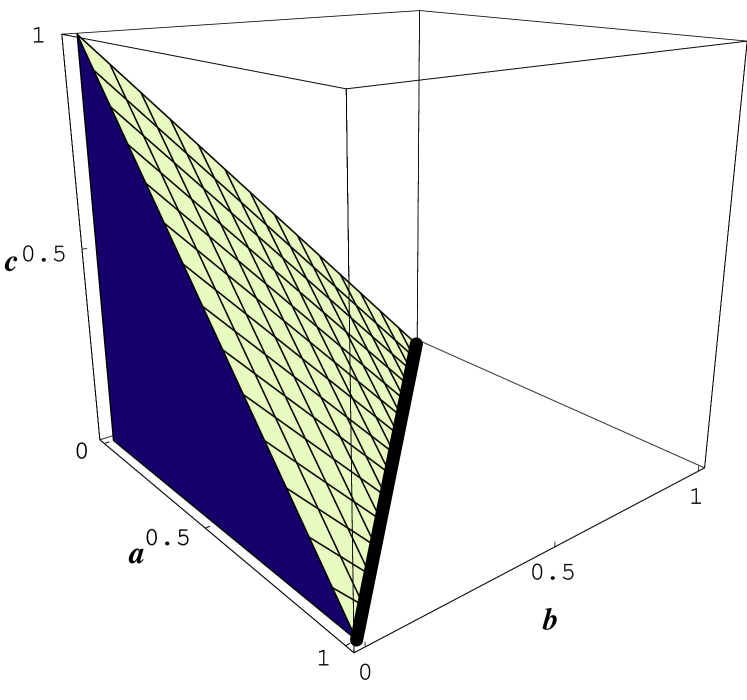
Figure 1.2: The target space containing points corresponding to the probability spaces respectively of the coin ${\cal P}^{\prime}_{\rm coin}$ along the line $a+b=1$ with constraint $(c,d)=(0,0)$ (heavy line), of the triangle ${\cal P}^{\prime}_{\rm triangle}$ along the surface $a+b+c=1$ with constraint $d=0$ (hashed surface), and of the square ${\cal P}^{\prime}_{\rm square}$ filling the volume $a+b+c+d=1$ (filled polygon). Note that points such as $(a,b,c)=(0.5,0.5,0)$ correspond to all three probability spaces and are only distinguished by which constraints are acting.

The interesting point about the target space is that many points, e.g. $(a,b,c,d)=(\frac{1}{2},\frac{1}{2},0,0)$, lie in all of the probability spaces of the coin, triangle, and square die and are only distinguished by which constraints are acting. That is, when this point is subject to the constraint $(cd)=(00)$, then it corresponds to the probability space ${\cal P}^{\prime}_{\rm coin}$ (and not to any other). Conversely, when this same point is subject to an imposed constraint $d=0$ then it corresponds to the probability space ${\cal P}^{\prime}_{\rm triangle}$. Finally, when no constraints apply then, and only then does this point correspond to the probability space of the square ${\cal P}^{\prime}_{\rm square}$. This means that it is not the probability values possessed by a point which determines its corresponding probability space but the probability values in combination with the constraints acting at that point.

It is now straightforward to use the isomorphically constrained target space to maximize the function $f$ over all embedded probability spaces using standard constrained optimization techniques. For instance, to optimize $f$ over points corresponding to the coin and subject to the constraint $(c,d)=(0,0)$ then either simply resolve the constraint via setting $c=d=0$ before the optimization begins, or simply evaluate the gradient of $f$ at all points $(a,b,0,0)$ in the direction of the unit vector $\frac{1}{\sqrt{2}}(1,-1,0,0)$ lying along the line $a+b=1$. In more detail, the function $f(a,b,c)$ has a directed gradient in the direction $\frac{1}{\sqrt{2}}(1,-1,0)$ of

$$\nabla f(a,b,c).\frac{1}{\sqrt{2}}(1,-1,0)=V^{2}\frac{1}{\sqrt{2}}\log\frac{b}{a}$$ (1.15)

using Eq. 1.2.1. The rate of change of $f$ with respect to the only remaining variable $a$ is given by

$$\frac{df}{da}=\sqrt{2}\nabla f.\frac{1}{\sqrt{2}}(1,-1,0).$$ (1.16)

Altogether, at points where $(a,b,c)=(a,1-a,0)$ this gives a directed gradient of

$$\frac{df}{da}=V^{2}\log\frac{1-a}{a}$$ (1.17)

which is optimized at $(a,b,c)=(\frac{1}{2},\frac{1}{2},0)$. An optimization over all three isomorphic constraints leads to the same outcomes as obtained previously in Eq. 1.2.1 with the same result. This completes the second optimization analysis and as promised, it is consistent with the results of the first.

The same is not true of the third optimization approach which produces results inconsistent with the first two. The reason we present this method is that it is in common use in game theory. The third optimization method commences by noting that the probability space of the square is complete in that it already “contains” all of probability spaces of the triangle and of the coin. This allows a square probability space to mimic a coin probability space by simply taking the limit $(c,d)\rightarrow(0,0)$. Similarly, the square mimics the triangle through the limit $d\rightarrow 0$. In turn, this means that an optimization over the space of the square is effectively an optimization over every choice of space within the square. Specifically, game theory discards constraints to model the choice between contained probability spaces. This optimization over the points of the square has already been completed above. When optimizing the function $f$ over the unconstrained points corresponding to the square, the maximum value is $f=\log(4)/36$ at $(a,b,c,d)=(\frac{1}{4},\frac{1}{4},\frac{1}{4},\frac{1}{4})$, and according to game theory, this is the best outcome when players have a choice between the coin, the triangle, or the square.

The optimum result obtained by the third optimization method, that used by game theory, conflicts with those found by the previous two methods as commonly used in probability theory. The difference arises as game theory models a choice between probability spaces by making players uncertain about the values of their probability parameters within any probability space. Consequently, their probability parameters are always subject to infinitesimal fluctuations, i.e. $c>0^{+}$ or $d>0^{+}$ always. These fluctuations alter the dimensions of the space which impacts on the calculation of the volume $V$ and alters the calculated gradient of the entropy. Game theory eschews the role of isomorphism constraints within probability spaces on the grounds that any such constraints restrict player uncertainty and hence their ability to choose between different probability spaces. The probability parameter fluctuations mean that players have access to all possible probability dimensions at all times so a single mixed space is the appropriate way to model the choice between contained probability spaces. In contrast, probability theory holds that the choice between probability spaces introduces player uncertainty about which space to use, but specifically does not introduce uncertainty into the parameters within any individual probability space. As a result, probability theory employs isomorphic constraints to ensure that the properties of each embedded probability space within the mixed space are unchanged.

The upshot is that a game theorist cannot evaluate the Entropy (or uncertainty) gradient of a coin toss while considering alternate die because uncertainty about which dice is used bleeds into the Entropy calculation. However, the probability theorist will distinguish between their uncertainty about which face of the coin will appear and their uncertainty about which dice is being used.

1.2.2 Alternate coin probability spaces

The preceding section has shown the importance of using isomorphism constraints to preserve the properties of the coin probability space ${\cal P}_{\rm coin}$ when embedded within larger spaces. However, isomorphism constraints must also be used in the very definition of a probability space. If a probability space is to be defined to match some physical apparatus, then a structure preserving isomorphic mapping must be established between the physical apparatus and the probability space. We illustrate this now by adopting several different probability spaces for a coin.

In the preceding sections, we have the physical coin as shown in Fig. 1.1 and its corresponding probability space as defined in Eq. 1.2.1. To reiterate,

$${\cal P}_{\rm coin}=\big{\{}x\in\{A,B\},\{a,b\}\big{\}}.$$ (1.18)

After taking account of the normalization constraint $b=1-a$, the gradient operator in this space is

$$\nabla=\hat{a}\frac{\partial}{\partial a}.$$ (1.19)

If we define a payoff via the random variable $\Pi(A)=0$ and $\Pi(B)=1$, then a gradient optimization gives

$$\nabla\langle\Pi\rangle = \nabla P(B)$$ (1.20)

$$= -\hat{a}$$

indicating that expected payoffs are maximized by setting $a=0$ as expected.

There are many very different formulations possible for the probability space of a simple two sided coin, and these are considered to be functionally identical only after the appropriate structure-preserving isomorphisms have been defined. Every alternative introduces a different parameterization which alters dimensionality and gradient operators and modifies the optimization algorithm. We illustrate this now.

Our coin could be optimized using a probability measure space ${\cal P}_{\rm coin}^{2}$ involving two uncorrelated coins, namely

$${\cal P}_{\rm coin}^{2}=\big{\{}(x,y)\in\{(0,0),(0,1),(1,0),(1,1)\},\{(1-p)(1-q),(1-p)q,p(1-q),pq\}\big{\}}.$$ (1.21)

An isomorphism can be defined by mapping event $A$ onto the event set $(x,y)\in\{(0,0),(1,1)\}$ and $B$ onto $(x,y)\in\{(0,1),(1,0)\}$. In this space, the gradient operator is

$$\nabla=\hat{p}\frac{\partial}{\partial p}+\hat{q}\frac{\partial}{\partial q}$$ (1.22)

and a gradient optimization of the expected payoff gives

$$\nabla\langle\Pi\rangle = \nabla P(B)$$ (1.23)

$$= \hat{p}(1-2q)+\hat{q}(1-2p).$$

This shows that when $q<\frac{1}{2}$ then payoffs are maximized by setting $p=1$ and conversely, when $p<\frac{1}{2}$ then payoffs are maximized by setting $q=1$.

Alternatively, the binary decision could be optimized using a continuously parameterized probability measure space ${\cal P}_{\rm coin}^{3}$. In this space, the choices $A$ and $B$ might be determined using a continuously distributed variable $u\in(-\infty,\infty)$ possessing a normally distributed probability distribution

$$P(u)=\frac{1}{\sqrt{2\pi}\sigma}e^{-\frac{1}{2}\frac{(u-\bar{u})^{2}}{\sigma^{2}}},$$ (1.24)

with mean $\bar{u}$, standard deviation $\sigma$, and variance $\sigma^{2}$. We introduce a new parameter, $p$, so outcome $A$ occurs with probability

$$P(A)=\frac{1}{\sqrt{2\pi}\sigma}\int_{-\infty}^{p}du\;e^{-\frac{1}{2}\frac{(u-\bar{u})^{2}}{\sigma^{2}}},$$ (1.25)

while outcome $B$ occurs with probability

$$P(B)=\frac{1}{\sqrt{2\pi}\sigma}\int_{p}^{\infty}du\;e^{-\frac{1}{2}\frac{(u-\bar{u})^{2}}{\sigma^{2}}}.$$ (1.26)

This space has only one probability parameter $p$ so the gradient operator is

$$\nabla=\hat{p}\frac{\partial}{\partial p},$$ (1.27)

and optimizing the expected payoff gives

$$\nabla\langle\Pi\rangle = \nabla\frac{1}{\sqrt{2\pi}\sigma}\int_{p}^{\infty}du\;e^{-\frac{1}{2}\frac{(u-\bar{u})^{2}}{\sigma^{2}}}$$ (1.28)

$$= -\nabla F(p),$$

where $F(p)$ is the cumulative normal distribution. As the cumulative normal distribution is monotonically increasing, $\nabla F(p)>0$, so the expected payoff is maximized by setting $p\rightarrow-\infty$ giving $P(B)=1$ as expected.

For a more extreme alternative, consider a quantum probability measure space ${\cal P}_{\rm coin}^{4}$ in which event $A$ corresponds to a measurement finding a two-state quantum system in its ground state, and event $B$ occurs when the measurement finds the system in its excited state. Writing the quantum system state as

$$|\Psi\rangle=\left[\begin{array}[]{c}a\\ \\ b\\ \end{array}\right],$$ (1.29)

where $a$ and $b$ are complex numbers satisfying $|a|^{2}+|b|^{2}=1$, then we have $P(A)=|a|^{2}$ and $P(B)=|b|^{2}$. In this space, the payoff is an operator

$$\Pi=\left[\begin{array}[]{cc}0&0\\ &\\ 0&1\\ \end{array}\right],$$ (1.30)

giving the expected payoff as

$$\langle\Pi\rangle = \langle\Psi|\Pi|\Psi\rangle$$ (1.31)

$$= |b|^{2}$$

$$= r^{2},$$

where in the last line we write $b=re^{i\theta}$ with real $0\leq r\leq 1$ and $0\leq\theta<2\pi$. Here, the expected payoff depends only on the single real variable $r$ so optimization is via the gradient operator

$$\nabla=\hat{r}\frac{\partial}{\partial r}$$ (1.32)

giving

$$\nabla\langle\Pi\rangle=2r.$$ (1.33)

As required, maximization requires setting $r=1$, with $\theta$ arbitrary.

For a last example, consider a probability space ${\cal P}_{\rm coin}^{5}$ which selects a number $u$ in the Cantor set ${\cal C}$ with uniform probability $P(u)$ such that when $u\leq p$ then event $A$ occurs while when $p<u$ then event $B$ occurs. The Cantor set ${\cal C}$ is interesting as it has an uncountably infinite number of members and yet has measure zero [13]. In this space, the expected payoff is

$$\langle\Pi\rangle = \sum_{u\in{\cal C}}P(u)\Pi(u)$$ (1.34)

$$= \sum_{u>p\in{\cal C}}P(u)$$

$$= 1-C(p),$$

where $C(p)$ is the cumulative probability distribution termed the Cantor function. Interestingly, the Cantor function is an example of a “Devil’s staircase”, a function which is continuous but not absolutely continuous everywhere, and is differentiable with derivative zero almost everywhere, and which maps the measure zero Cantor set continuously onto the measure one set $[0,1]$ [13]. As with the normal distribution example above, the Cantor function is nondecreasing allowing an intuitive maximization of the expected payoff via the gradient operator

$$\nabla=\frac{\partial}{\partial p}$$ (1.35)

giving

$$\nabla\langle\Pi\rangle=-\frac{dC(p)}{dp}.$$ (1.36)

As the cumulative normal distribution is nondecreasing, we have $\frac{dC(p)}{dp}\geq 0$ so the expected payoff is maximized by setting $p=0$. This intuitive ansatz suffices for our purposes here.

Lastly, the player is of course, not restricted to using only simple probability measure spaces, and more complicated spaces can be considered. In fact, players will most likely use a pseudo-random number generator consisting of the correlated dynamical interactions of some millions (or more) of electronic components in a computer. It is only the correlations of these millions of variables that allows a dimensionality reduction to the few variables required to model the player’s chosen probability space. Isomorphisms underlie the dimensionality reductions of random number generators.

To summarize, optimizing an expected payoff first requires the adoption of a suitable probability measure space, and it is only the adoption of such a space that permits the definition of gradient operators and the expected payoff functions allowing the optimization to be completed. These steps involve establishing an isomorphic mapping from the physically modeled space to the probability space which is property conserving. Of course, should the probability space then be embedded within any other probability space, these properties must still be conserved, and this will require additional isomorphic constraints.

Figure 1.3: A four-sided square probability space where joint variables $x$ and $y$ take values $(x,y)\in\{(0,0),(0,1),(1,0),(1,1)\}$ with respective probabilities $(a,b,c,d)$.

1.2.3 Joint probability space optimization

We will briefly now examine isomorphisms between the joint probability spaces of two arbitrarily correlated random variables. In particular, we consider two random variables $x,y$ as appear on the square dice of Fig. 1.3 with probability space

$${\cal P}_{\rm square} = \big{\{}(x,y)\in\{(0,0),(0,1),(1,0),(1,1)\},\{a,b,c,d\}\big{\}}.$$ (1.37)

The correlation between the $x$ and $y$ variables is

$$\rho_{xy} = \frac{\langle xy\rangle-\langle x\rangle\langle y\rangle}{\sigma_{x}\sigma_{y}}$$ (1.38)

$$= \frac{ad-bc}{\sqrt{(c+d)(a+b)(b+d)(a+c)}}.$$

Here, $\sigma_{x}$ and $\sigma_{y}$ are the respective standard deviations of the $x$ and $y$ variables.

The space ${\cal P}_{\rm square}$ of course contains many embedded or contained spaces. We will separately consider the case where $x$ and $y$ are perfectly correlated, and where they are independent. As noted previously, there are two distinct ways for these spaces to be contained within ${\cal P}_{\rm square}$, namely using isomorphism constraints or using limit processes. These two ways give the respective definitions for the perfectly correlated case

$${\cal P}_{\rm corr} = \left.\left\{(x,y)\in\{(0,0),(0,1),(1,0),(1,1)\},\{a,b,c,d\}\right\}\right|_{b=c=0}$$

$${\cal P}^{\prime}_{\rm corr} = \lim_{(bc)\rightarrow(00)}\left\{(x,y)\in\{(0,0),(0,1),(1,0),(1,1)\},\{a,b,c,d\}\right\}$$ (1.39)

and for the independent case

$${\cal P}_{\rm ind} = \left.\left\{(x,y)\in\{(0,0),(0,1),(1,0),(1,1)\},\{a,b,c,d\}\right\}\right|_{ad=bc}$$

$${\cal P}^{\prime}_{\rm ind} = \lim_{ad\rightarrow bc}\left\{(x,y)\in\{(0,0),(0,1),(1,0),(1,1)\},\{a,b,c,d\}\right\}.$$ (1.40)

Here, all spaces satisfy the normalization constraint $a+b+c+d=1$, which we typically resolve using $d=1-a-b-c$. The gradient operator in the probability space of the square dice with probability parameters $(a,b,c)$ is

$$\nabla=\hat{a}\frac{\partial}{\partial a}+\hat{b}\frac{\partial}{\partial b}+\hat{c}\frac{\partial}{\partial c},$$ (1.41)

where a hat indicates a unit vector in the indicated direction. Evaluating any function dependent on a gradient or completing an optimization task using either isomorphic constraints or limit processes can naturally result in different outcomes as we now illustrate.

Perfectly correlated probability spaces

We first consider the case where the $x$ and $y$ variables are perfectly correlated in the spaces ${\cal P}_{\rm corr}$ with isomorphism constraints or ${\cal P}^{\prime}_{\rm corr}$ using limit processes.

The maximum achievable joint entropy [12] for our two perfectly correlated variables obviously occurs at the point where they are equiprobable. This can be found by evaluating the gradient of the joint entropy function

$$E_{xy}(a,b,c) = -\sum_{xy}P_{xy}\log P_{xy}$$

$$= -a\log a-b\log b-c\log c-(1-a-b-c)\log(1-a-b-c)$$

giving respective gradients in the ${\cal P}_{\rm corr}$ and ${\cal P}^{\prime}_{\rm corr}$ spaces of

$$\nabla E_{xy}|_{b=c=0} = -\hat{a}\log\left(\frac{a}{1-a}\right)$$

$$\nabla E_{xy} = -\hat{a}\log\left(\frac{a}{1-a-b-c}\right)-\hat{b}\log\left(\frac{b}{1-a-b-c}\right)-\hat{c}\log\left(\frac{c}{1-a-b-c}\right)$$

$$\lim_{(bc)\rightarrow(00)}\nabla E_{xy} = {\rm undefined}.$$ (1.43)

Equating these gradients to zero locates the maximum at $(a,b,c)=(\frac{1}{2},0,0)$ in ${\cal P}_{\rm corr}$ and at $(a,b,c)=(\frac{1}{4},\frac{1}{4},\frac{1}{4})$ in ${\cal P}^{\prime}_{\rm corr}$.

The Fisher Information is defined in terms of probability space gradients as the amount of information obtained about a probability parameter from observing any event [12]. Writing $(a,b,c)=(p_{1},p_{2},p_{3})$, the Fisher Information is a matrix with elements $i,j\in\{1,2,3\}$ with

$$F_{ij} = \sum_{xy}P_{xy}\left(\frac{\partial}{\partial p_{i}}\log P_{xy}\right)\left(\frac{\partial}{\partial p_{j}}\log P_{xy}\right).$$ (1.44)

When isomorphically constrained in the space ${\cal P}_{\rm corr}$, the Fisher Information is $F_{ij}|_{b=c=0}$ with the only nonzero term being

$$F_{11} = (1-a)\left[\hat{a}\frac{\partial}{\partial a}\log(1-a)\right]^{2}+a\left[\hat{a}\frac{\partial}{\partial a}\log a\right]^{2}$$ (1.45)

$$= \frac{1}{a(1-a)}$$

This means that the smaller the Variance the more the information obtained about $a$. In the unconstrained space ${\cal P}^{\prime}_{\rm corr}$, the Fisher Information is a very different, $3\times 3$ matrix.

Probability parameter gradients also allow estimation of probability parameters by locating points where the Log Likelihood function is maximized $\nabla\log L=0$ [12]. This evaluation takes very different forms in the isomorphically constrained space ${\cal P}_{\rm corr}$ and the unconstrained space ${\cal P}^{\prime}_{\rm corr}$. The likelihood function estimates probability parameters from the observation of $n$ trials with $n_{a}$ appearances of event $(x,y)=(0,0)$, $n_{b}$ appearances of event $(x,y)=(0,1)$, $n_{c}$ appearances of event $(x,y)=(1,0)$, and $n_{d}$ appearances of event $(x,y)=(1,1)$. We have $n_{a}+n_{b}+n_{c}+n_{d}=n$, giving the Likelihood function

$$L=f(n_{a},n_{b},n_{c},n)a^{n_{a}}b^{n_{b}}c^{n_{c}}(1-a-b-c)^{n-n_{a}-n_{b}-n_{c}}$$ (1.46)

where $f(n_{a},n_{b},n_{c},n)$ gives the number of combinations. The optimization proceeds by evaluating the gradient of the Log Likelihood function. When isomorphically constrained in the space ${\cal P}_{\rm corr}$, the gradient of the Log Likelihood function is

$$\nabla\log L|_{b=c=0}=\hat{a}\left[\frac{n_{a}}{a}-\frac{n-n_{a}}{1-a}\right],$$ (1.47)

which equated to zero gives the optimal estimate at $a=n_{a}/n$ and $n_{b}=n_{c}=0$ as expected. Conversely, when unconstrained in the space ${\cal P}^{\prime}_{\rm corr}$, the gradient of the Log Likelihood function evaluates as

$$\nabla\log L = \hat{a}\left[\frac{n_{a}}{a}-\frac{n-n_{a}-n_{b}-n_{c}}{1-a-b-c}\right]+\hat{b}\left[\frac{n_{b}}{b}-\frac{n-n_{a}-n_{b}-n_{c}}{1-a-b-c}\right]$$ (1.48)

$$\hskip 56.9055pt+\hat{c}\left[\frac{n_{c}}{c}-\frac{n-n_{a}-n_{b}-n_{c}}{1-a-b-c}\right].$$

This is obviously a very different result. However, in our case the same estimated outcomes can be achieved in both spaces. For example, if an observation of $n$ trials shows $n_{a}$ instances of $(x,y)=(0,0)$ and $n-n_{a}$ instances of $(x,y)=(1,1)$ then both constrained and unconstrained approaches give the best estimates of the probability parameters of $(a,b,c,d)=(\frac{n_{a}}{n},0,0,1-\frac{n_{a}}{n})$.

Finally, when $x$ and $y$ are perfectly correlated it is necessarily the case that expectations satisfy $\langle x\rangle-\langle y\rangle=0$, that variances satisfy $V(x)-V(y)=0$, that the joint entropy is equal to the entropy of each variable so $E_{xy}-E_{x}=0$, and that finally, the correlation between these variables satisfies $\rho_{xy}-1=0$. In the unconstrained probability space ${\cal P}^{\prime}_{\rm corr}$, the expectation, variance, and entropy relations of interest evaluate as

$$\langle x\rangle-\langle y\rangle = c-b$$

$$V(x)-V(y) = (c-b)(a-d)$$ (1.49)

$$E_{x} = -\left[(a+b)\log(a+b)+(1-a-b)\log(1-a-b)\right]$$

$$E_{xy} = -\left[a\log a+b\log b+c\log c+(1-a-b-c)\log(1-a-b-c)\right].$$

These functions lead to gradient relations in the ${\cal P}_{\rm corr}$ and ${\cal P}^{\prime}_{\rm corr}$ spaces of:

$$\nabla\left[\langle x\rangle-\langle y\rangle\right]|_{b=c=0} = 0$$

$$\lim_{(bc)\rightarrow(00)}\nabla\left[\langle x\rangle-\langle y\rangle\right] = -\hat{b}+\hat{c}$$

$$\nabla\left[V(x)-V(y)\right]|_{b=c=0} = 0$$

$$\lim_{(bc)\rightarrow(00)}\nabla\left[V(x)-V(y)\right] = (1-2a)\hat{b}-(1-2a)\hat{c}$$

$$\nabla\left[E_{xy}-E_{x}\right]|_{b=c=0} = 0$$

$$\lim_{(bc)\rightarrow(00)}\nabla\left[E_{xy}-E_{x}\right] \neq {\rm undefined}$$

$$\nabla\rho_{xy}|_{b=c=0} = 0$$

$$\nabla\rho_{xy} \neq 0.$$ (1.50)

Obviously, taking the limit $(b,c)\rightarrow(0,0)$ does not reduce the limit equations to the required relations.

Independent probability spaces

We next consider the case where the $x$ and $y$ variables are independent using the spaces ${\cal P}_{\rm ind}$ with isomorphism constraints or ${\cal P}^{\prime}_{\rm ind}$ with limit processes.

When random variables are independent, then their joint probability distribution is separable for every allowable probability parameter of ${\cal P}_{\rm ind}$ or ${\cal P}^{\prime}_{\rm ind}$. This means the gradient of this separability property must be invariant across these probability spaces. That is, we must have $P_{xy}=P_{x}P_{y}$ and hence $\nabla\left[P_{xy}-P_{x}P_{y}\right]=0$. Similarly, separability requires we also satisfy $\nabla\left[\langle xy\rangle-\langle x\rangle\langle y\rangle\right]=0$. Further, every independent space must have conditional probabilities equal to marginal probabilities and so satisfy $\nabla\left[P_{x|y}-P_{x}\right]=0$. Finally, two independent variables have joint entropy equal to the sum of the individual entropies so every independent space must satisfy $\nabla\left[E_{xy}-E_{x}-E_{y}\right]=0$. These relations evaluate differently in either ${\cal P}_{\rm ind}$ with isomorphism constraints or ${\cal P}^{\prime}_{\rm ind}$ with limit processes. For the square die under consideration, we have probabilities and expectations of

$$P_{xy}(00)-P_{x}(0) = ad-bc$$

$$\langle xy\rangle-\langle x\rangle\langle y\rangle = ad-bc$$

$$P_{x|y}(0|0)-P_{x}(0) = \frac{ad-bc}{a+c},$$ (1.51)

and entropies of

$$E_{x} = -(a+b)\log(a+b)-(1-a-b)\log(1-a-b)$$

$$E_{y} = -(a+c)\log(a+c)-(1-a-c)\log(1-a-c)$$

$$E_{xy} = -a\log a-b\log b-c\log c-d\log d.$$ (1.52)

The resulting gradients are

$$\nabla\left[P_{xy}(00)-P_{x}(0)P_{y}(0)\right]|_{ad=bc} = 0$$

$$\lim_{ad\rightarrow bc}\nabla\left[P_{xy}(00)-P_{x}(0)P_{y}(0)\right] = \lim_{ad\rightarrow bc}\nabla(ad-bc)\neq 0$$

$$\nabla\left[\langle xy\rangle-\langle x\rangle\langle y\rangle\right]|_{ad=bc} = 0$$

$$\lim_{ad\rightarrow bc}\nabla\left[\langle xy\rangle-\langle x\rangle\langle y\rangle\right] = \lim_{ad\rightarrow bc}\nabla(ad-bc)\;\neq\;0$$

$$\nabla\left[P_{x|y}(0|0)-P_{x}(0)\right]|_{ad=bc} = 0$$

$$\lim_{ad\rightarrow bc}\nabla\left[P_{x|y}(0|0)-P_{x}(0)\right] = \lim_{ad\rightarrow bc}\nabla\left[\frac{ad-bc}{a+c}\right]\;\neq\;0$$

$$\nabla\left[E_{xy}-E_{x}-E_{y}\right]|_{ad=bc} = 0$$

$$\lim_{ad\rightarrow bc}\nabla\left[E_{xy}-E_{x}-E_{y}\right] =$$

$$\lim_{ad\rightarrow bc}\nabla\left\{a\log\left[\frac{d}{a}\frac{a-ad+bc}{d-ad+bc}\right]+b\log\left[\frac{d}{b}\frac{b+ad-bc}{d-ad+bc}\right]+\right.$$

$$\left.c\log\left[\frac{d}{c}\frac{c+ad-bc}{d-ad+bc}\right]+\log\left[\frac{d-ad+bc}{d}\right]\right\}\;\neq\;0.$$

1.2.4 Entropy maximization

The joint entropy $E_{xy}$ reflects the uncertainty between the $x$ and $y$ variables. According to probability theory, this uncertainty does not include any uncertainty about which probability space is being chosen, while conversely, according to game theory the uncertainty between these variables increases when it includes additional uncertainty about which probability space is being chosen.

We now present a numerical investigation of how to determine the maximum joint entropy $E_{xy}$ of embedded probability states featuring possibly correlated variables $x$ and $y$ as depicted in Fig. 1.3. The joint entropy is

$$E_{xy}(a,b,c)=-\sum_{xy}P_{xy}\log P_{xy}.$$ (1.54)

Using isomorphism constraints, the maximization problem is

$$\max\left.E_{xy}\right|_{\rho_{xy}=\bar{\rho}}$$ (1.55)

for all $\bar{\rho}\in[-1,1]$. Here, the correlation function between $x$ and $y$ is given by the later Eq. 2.11. This equation can be inverted to solve for the variable $r$ as a function of $p$, $q$, and the constant correlation $\bar{\rho}$, and the result $r_{+}(p,q,\bar{\rho})$ is given in Eq. 3.10. A numerical optimization then generates the maximum entropy value for every correlation state $\bar{\rho}$ with the results shown in Fig. 1.4. As expected, the presence of isomorphism constraints ensures the entropy ranges from a minimum of $\log 2$ up to a maximum of $2\log 2$.

In contrast, when the joint entropy is maximized over the entire space using the techniques of game theory, then a single maximum outcome is achieved giving the maximum entropy in the absence of isomorphism constraints. This line is also shown in Fig. 1.4 as the constant at $E_{xy,{\rm max}}=2\log 2$.

Figure 1.4: Maximizing the joint entropy of two correlated random variables $x,y\in\{0,1\}$. Without isomorphism constraints, the maximum entropy is equal to $2\log 2$ (dashed line). However, when subject to isomorphism constraints, the simplex will exactly reproduce the different maximum entropy states of each of its embedded probability spaces (solid line).

1.2.5 Continuous bivariate Normal spaces

The above results are general. When source probability spaces are embedded within target probability spaces, then the use of isomorphic mapping constraints will preserve all properties of the embedded spaces. Conversely, when constraints are not used then some of the properties of the embedded spaces will not be preserved in general. We illustrate this now using normally distributed continuous random variables.

Consider two normally distributed continuous independent random variables $x$ and $y$ with $x,y\in(-\infty,\infty)$. When independent, these variables have a joint probability distribution $P_{xy}$ which is continuous and differentiable in six variables, $P_{xy}(x,\mu_{x},\sigma_{x},y,\mu_{y},\sigma_{y})$ where the respective means are $\mu_{x}$ and $\mu_{y}$ and the variances are $\sigma_{x}^{2}$ and $\sigma_{y}^{2}$. The marginal distributions are $P_{x}(x,\mu_{x},\sigma_{x})$ and $P_{y}(y,\mu_{y},\sigma_{y})$. In particular, we have

$$P_{xy} = \frac{1}{2\pi\sigma_{x}\sigma_{y}}e^{-\frac{1}{2}\left[\frac{(x-\mu_{x})^{2}}{\sigma_{x}^{2}}+\frac{(y-\mu_{y})^{2}}{\sigma_{y}^{2}}\right]}$$

$$P_{x} = \frac{1}{\sqrt{2\pi}\sigma_{x}}e^{-\frac{1}{2}\frac{(x-\mu_{x})^{2}}{\sigma_{x}^{2}}}$$

$$P_{y} = \frac{1}{\sqrt{2\pi}\sigma_{y}}e^{-\frac{1}{2}\frac{(y-\mu_{y})^{2}}{\sigma_{y}^{2}}}.$$ (1.56)

The conditional distribution for $x$ given some value of $y$ is

$$P_{x|y}=\frac{1}{\sqrt{2\pi}\sigma_{x}}e^{-\frac{1}{2}\frac{(x-\mu_{x})^{2}}{\sigma_{x}^{2}}}.$$ (1.57)

These independent joint distributions can now be embedded into an enlarged distribution representing two potentially correlated normally distributed variables $x$ and $y$. This enlarged distribution $P^{\prime}_{xy}(x,\mu_{x},\sigma_{x},y,\mu_{y},\sigma_{y},\rho)$ differs from $P_{xy}$ in its dependence on the correlation parameter $\rho_{xy}=\rho$ with $\rho\in(-1,1)$. This distribution is continuous and differentiable in seven variables. The joint distribution is

$$P^{\prime}_{xy} = \frac{1}{2\pi\sigma_{x}\sigma_{y}\sqrt{1-\rho^{2}}}e^{-\frac{1}{2(1-\rho^{2})}\left[\frac{(x-\mu_{x})^{2}}{\sigma_{x}^{2}}-\frac{2\rho(x-\mu_{x})(y-\mu_{y})}{\sigma_{x}\sigma_{y}}+\frac{(y-\mu_{y})^{2}}{\sigma_{y}^{2}}\right]}.$$ (1.58)

The marginal distributions for the correlated case are identical to those of the independent space so $P^{\prime}_{x}=P_{x}$ and $P^{\prime}_{y}=P_{y}$. The conditional distribution for $x$ given some value of $y$ is

$$P^{\prime}_{x|y}=\frac{1}{\sqrt{2\pi(1-\rho^{2})}\sigma_{x}}e^{-\frac{1}{2(1-\rho^{2})}\frac{(x-\bar{\mu}_{x})^{2}}{\sigma_{x}^{2}}},$$ (1.59)

where the new conditioned mean is

$$\bar{\mu}_{x}=\mu_{x}+\rho\frac{\sigma_{x}}{\sigma_{y}}(y-\mu_{y}).$$ (1.60)

An isomorphic embedding requires that the unit probability subset of $P_{xy}$ be mapped onto the unit probability subset of $P^{\prime}_{xy}$ and this is achieved by imposing an external constraint that $\rho=0$ in the enlarged space. Hence, we expect $\left.P^{\prime}_{xy}\right|_{\rho=0}=P_{xy}$. It is readily confirmed that when the isomorphism constraint is imposed on the enlarged distribution all properties are preserved, while this is not the case in the absence of the constraint. The gradient operator $\nabla$ is now a function of seven variables

$$\nabla = \frac{\partial}{\partial x}\hat{x}+\frac{\partial}{\partial y}\hat{y}+\frac{\partial}{\partial\mu_{x}}\hat{\mu}_{x}+\frac{\partial}{\partial\mu_{y}}\hat{\mu}_{y}+\frac{\partial}{\partial\sigma_{x}}\hat{\sigma}_{x}+\frac{\partial}{\partial\sigma_{y}}\hat{\sigma}_{y}+\frac{\partial}{\partial\rho}\hat{\rho}.$$ (1.61)

The probability distributions must satisfy a number of gradient relations, but we have:

$$\left.\nabla\left[P^{\prime}_{xy}-P^{\prime}_{x}P^{\prime}_{y}\right]\right|_{\rho=0} = 0$$

$$\lim_{\rho\rightarrow 0}\nabla\left[P^{\prime}_{xy}-P^{\prime}_{x}P^{\prime}_{y}\right] = \hat{\rho}\lim_{\rho\rightarrow 0}\frac{\partial}{\partial\rho}P^{\prime}_{xy}\neq 0$$

$$\left.\nabla\left[P^{\prime}_{x|y}-P^{\prime}_{x}\right]\right|_{\rho=0} = 0$$

$$\lim_{\rho\rightarrow 0}\nabla\left[P^{\prime}_{x|y}-P^{\prime}_{x}\right] = \hat{\rho}\lim_{\rho\rightarrow 0}\frac{\partial}{\partial\rho}P^{\prime}_{x|y}\neq 0.$$ (1.62)

Similarly, the expectations of functions of the $x$ and $y$ variables must also satisfy a number of gradient relations. As expectations integrate over the $x$ and $y$ variables, the gradient operator is a function of only five variables now,

$$\nabla=\frac{\partial}{\partial\mu_{x}}\hat{\mu}_{x}+\frac{\partial}{\partial\mu_{y}}\hat{\mu}_{y}+\frac{\partial}{\partial\sigma_{x}}\hat{\sigma}_{x}+\frac{\partial}{\partial\sigma_{y}}\hat{\sigma}_{y}+\frac{\partial}{\partial\rho}\hat{\rho}.$$ (1.63)

We have

$$\left.\nabla\left[\langle xy\rangle^{\prime}-\langle x\rangle^{\prime}\langle y\rangle^{\prime}\right]\right|_{\rho=0} = 0$$

$$\lim_{\rho\rightarrow 0}\nabla\left[\langle xy\rangle^{\prime}-\langle x\rangle^{\prime}\langle y\rangle^{\prime}\right] = \hat{\rho}\lim_{\rho\rightarrow 0}\frac{\partial}{\partial\rho}\langle xy\rangle^{\prime}\neq 0.$$

1.2.6 Quantum probability spaces

As noted above, the use of isomorphic mappings to preserve the properties of probability spaces is general. As a last illustration, we show the use of isomorphic mappings when applied to quantum probability spaces.

Suppose a quantum probability space is to be embedded within another enlarged quantum probability space. (See [14] for an overview of quantum information theory including quantum information geometry.) An $N$ level quantum system has von Neumann entropy defined as

$$E_{N}=-{\rm tr}\hat{R}_{N}\log\hat{R}_{N}$$ (1.64)

where here $\hat{R}_{N}$ is the quantum density matrix and ${\rm tr}$ indicates a trace operation applied to a matrix. Supposing that matrix $D$ diagonalizes the density matrix so $D\hat{R}_{N}D^{\dagger}$ is diagonal, and that its eigenvalues are $\lambda_{i}$ for $1\leq i\leq N$, we have

$$E_{N}=-\sum_{i=1}^{N}\lambda_{i}\log\lambda_{i}.$$ (1.65)

The eigenvalue $\lambda_{i}$ specifies the occupancy probability of the $i^{\rm th}$ level. Hence, maximizing the $N$-level system entropy requires that $\lambda_{i}=1/N$ for all $i$. Consequently, a two level quantum system maximizes its entropy $E_{2}$ when the density matrix is an equiprobable mixture equal to half of the two level identity matrix, $\hat{R}_{2}=1/2I_{2}$, while a three level quantum system maximizes its entropy $E_{3}$ when the density matrix is an equiprobable mixture of $\hat{R}_{3}=1/3I_{3}$.

Now, if the two level system were isomorphically embedded within a three level system, then the two level system entropy $E_{2}$ is properly maximized only when isomorphism constraints are used to decouple the third level so that it plays no part in the optimization. This is achieved by using an isomorphism constraint $\lambda_{3}=0$ to decouple and remove the third level from the system. That is, the optimization taking account of an isomorphism constraint $\nabla_{3}E_{3}|_{\lambda_{3}=0}=0$ will determine the correct maximum value for $E_{2}$. However, a failure to use an isomorphism constraint will locate an incorrect maximum point via $\lim_{\lambda_{3}\rightarrow 0}\nabla_{3}E_{3}$. We have

$$\nabla_{2}E_{2}=\nabla_{3}E_{3}|_{\lambda_{3}=0}\neq\lim_{\lambda_{3}\rightarrow 0}\nabla_{3}E_{3}.$$ (1.66)

Isomorphism constraints must be used to properly embed one quantum probability space within another.

Figure 1.5: (a) An affine transformation of correlated variables $x$ and $y$ generates new orthogonal variables $u=x+y$ and $v=x-y$ which are uncorrelated. (b) When $x$ and $y$ are perfectly correlated, $v=0$ and $u$ is the only free variable and dimensionality is reduced. Optimization solutions must lie on the $u$-axis satisfying the constraint $x=y$.

1.2.7 Perfect correlation reduces dimensionality

Standard probability theory holds that when two variables $x$ and $y$ are known to be perfectly correlated, then $P(x,y)=P(x)P(y|x)=P(x)$. That is, any optimization which involves the joint distribution $P(x,y)$ does not involve two dimensions but only one as $x=y$. Perfect correlation reduces dimensionality which alters the gradient operators which in turn can alter optima.

Probability theory takes account of this dimensionality reduction when using Affine variable transforms. Typical presentations of probability theory hold that “any two real-valued random variables $x$ and $y$ whose mean values and variances exist may be represented as an Affine transformation of a pair of uncorrelated random variables” [15]. Such statements, carelessly interpreted, would indeed suggest that perfect correlations involve no reduction in the number of variables. Writing the respective mean values as $\langle x\rangle$ and $\langle y\rangle$, and defining the translated variables

$$x^{*} = x-\langle x\rangle$$

$$y^{*} = y-\langle y\rangle,$$ (1.67)

then an affine transformation can always be used to define two new variables

$$u = x^{*}+y^{*}$$

$$v = x^{*}-y^{*}.$$ (1.68)

These variables each have mean zero, $\langle u\rangle=\langle v\rangle=0$, and are uncorrelated as

$${\rm cov}(u,v)=\langle uv\rangle=0.$$ (1.69)

The zero covariance results from the orthogonality of the random variables $u$ and $v$ in a suitable $L^{2}$ vector space, while the possibly correlated original variables are generated from the inverse affine transformation

$$x = \sigma_{x}x^{*}+\langle x\rangle\;=\;\frac{\sigma_{x}}{2}(u+v)+\langle x\rangle$$

$$y = \sigma_{y}y^{*}+\langle y\rangle\;=\;\frac{\sigma_{y}}{2}(u-v)+\langle y\rangle,$$ (1.70)

where here, $\sigma_{z}$ is the standard deviation of variable $z\in\{x,y\}$.

If the $x$ and $y$ variables are perfectly correlated, then $v$ is identically zero and $u$ is the only surviving variable. Perfect correlations reduce the dimensionality of the optimization space and probability theory preserves the dimensionality of perfectly correlated variables when using Affine transforms. (See Fig. 1.5.)

A similar preservation of dimensionality occurs in the Hotelling transform, a discrete version of the Karhunen-Loève transform [16]. This transform can also be used to map the probability space of two uncorrelated centered variables $(u,v)$ into the probability space of two correlated centered variables $(x,y)$. If the state of correlation between $x$ and $y$ is $\rho$, then the Hotelling transform is implemented via

$$\left[\begin{array}[]{c}x\\ y\end{array}\right]=\left[\begin{array}[]{cc}1&0\\ \rho&\sqrt{1-\rho^{2}}\end{array}\right]\;\left[\begin{array}[]{c}u\\ v\end{array}\right].$$ (1.71)

Then, whenever the $x$ and $y$ variables are not perfectly correlated both the $(u,v)$ and $(x,y)$ probability spaces are two dimensional. However, when $\rho=1$ and $x$ and $y$ are perfectly correlated, then the mapping matrix becomes singular and non-invertible ensuring that $x=y=u$ so that the $x$ and $y$ probability space is one dimensional even while the $u$ and $v$ probability space is two dimensional. Probability theory again acts to preserve the dimensionality of the joint probability space of perfectly correlated variables.

1.2.8 Example isomorphic functions

There are different ways to embed a smaller source function within an enlarged target function which can preserve different amounts of the structure of the source function within the target function. Consider for example, mapping a 1-dimensional function $f(x)$ into a 2-dimensional function $g(x,y)$ along the line $y=x$ so that $f(x)=g(x,x)$. One way to implement this assignment is to use limit processes constraining most of the neighbourhood of $g(x,y)$ in the vicinity of the line $y=x$ to satisfy

$$\lim_{y\rightarrow x}g(x,y)=f(x).$$ (1.72)

Another way to do this is to ignore the values of $g(x,y)$ away from the line $y=x$ and simply use externally imposed constraints forcing the assignment on the line via

$$g(x,y)|_{y=x}=f(x).$$ (1.73)

This approach does not care about values $g(x,y)$ when $x\neq y$. The question then is, under what circumstances can $\lim_{y\rightarrow x}g(x,y)$ or $g(x,y)|_{y=x}$ be used to examine the properties of $f(x)$.

Hereinafter, for concreteness we will consider the simplified example functions $f(x)=x^{2}$ and $g(x,y)=xy$. Each of the implementations, $\lim_{y\rightarrow x}g(x,y)$ or $g(x,y)|_{y=x}$, have different domains (dom) in each space, and hence different integration volume elements ($dv$)

$$\begin{array}[]{c|ccc}&\hskip 28.45274ptf(x)&\hskip 28.45274pt\lim_{y\rightarrow x}g(x,y)&\hskip 28.45274ptg(x,y)|_{y=x}\\ \hline\cr{\rm dom}&\Re&\Re\times\Re&\Re\\ dv&dx&dx\;dy&dx.\\ \end{array}$$ (1.74)

The different dimensionalities of the domains impacts on any attempt to change variables within each space. The rank of the change of variable transforms ($A$) and the dimensionality of the Jacobian matrices ($J$) in each space are

$$\begin{array}[]{c|ccc}&\hskip 28.45274ptf(x)&\hskip 28.45274pt\lim_{y\rightarrow x}g(x,y)&\hskip 28.45274ptg(x,y)|_{y=x}\\ \hline\cr{\rm rank}(A)&1&2&1\\ {\rm dim}(J)&1&2&1.\\ \end{array}$$ (1.75)

These differences impact on the evaluation of other properties such as gradients, which should evaluate as

$$\nabla f(x)=2x\hat{x}$$ (1.76)

where a hatted variable denotes a unit vector in the indicated direction. In contrast, the gradient evaluated using a limit assignment gives

$$\nabla g(x,x)=\lim_{y\rightarrow x}\nabla g(x,y)=x(\hat{x}+\hat{y}),$$ (1.77)

which does not satisfy the required relation. Conversely, the use of an externally imposed constraint ensures

$$\nabla g(x,y)|_{y=x}=\nabla g(x,x)=2x\hat{x}$$ (1.78)

as required.

In summary, the definitions

$$f(x)=g(x,y)|_{y=x}=\lim_{y\rightarrow x}g(x,y),$$ (1.79)

do not generally carry over to the gradient relations, as

$$\nabla f(x)=\nabla g(x,y)|_{y=x}\neq\lim_{y\rightarrow x}\nabla g(x,y),$$ (1.80)

This results as the limit process $f(x)=\lim_{y\rightarrow x}g(x,y)$ treats the $x$ and $y$ variables as being independent and simply evaluates desired quantities at points $(x,y)$ lying on the line $y=x$. In contrast, the constraint $f(x)=g(x,y)|_{y=x}$ enforces a functional relation between the $x$ and $y$ variables which preserves all the structures of $f(x)$ within $g(x,x)$. It is well understood that any functional relation between the variables of a function will impact on the properties of that function. Such functional relations must be preserved whenever that function is mapped into a different space. The need to take account of such functional relations is a standard part of routine optimization techniques such as differentiation via any of the chain rule, Lagrangian multipliers, or directed vector gradients.

A number of standard techniques exist for evaluating the gradient $f^{\prime}(x)$ using the constrained function $g(x,y)|_{y=x}$. For instance, the chain rule can be applied to the functions $g(x,y)$ and $y(x)=x$ giving

$$f^{\prime}(x) = \frac{\partial g}{\partial x}+\frac{\partial g}{\partial y}\frac{dy}{dx}$$ (1.81)

$$= 2x\hat{x}.$$

Another common alternative is by using Lagrange multipliers in which $f^{\prime}(x)=L^{\prime}(x)$ with

$$L(x,y,\lambda)=xy-\lambda(y-x)$$ (1.82)

and

$$\frac{\partial L}{\partial x} = (y+\lambda)\hat{x}$$

$$\frac{\partial L}{\partial y} = (x-\lambda)\hat{y}$$

$$\frac{\partial L}{\partial\lambda} = (x-y)\hat{\lambda}.$$ (1.83)

Equating the last two lines to zero gives the required constraints $y=x$ and $\lambda=x$ ensuring $f^{\prime}(x)=L^{\prime}(x)$. A final way to perform this constrained optimization is to use directed vector gradients where

$$f^{\prime}(x)=\lim_{y\rightarrow x}\nabla g(x,y).v.\sqrt{2}$$ (1.84)

with $v=(\hat{x}+\hat{y})/\sqrt{2}$. Here, $v$ is normalized and the extra factor of $\sqrt{2}$ properly calculates changes in the $x$ direction. This gives the magnitude of the gradient as $f^{\prime}(x)=2x$ as required.

There are two ways to embed the function $f(x)$ within the surface $g(x,y)$ using either a limit process or an externally imposed constraint. The limit process fails to preserve many of the properties of the source function within the target function. Conversely, the external constraint does ensure that all source function structures are preserved within the target function—dimensionality, gradient, and so on. In general, it is not possible to embed a smaller space within a larger space and preserve gradients and optimization outcomes without the use of constraints. These constraints reflect the use of isomorphic mappings to preserve the properties of the source space with the target space [17].

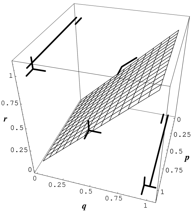
Figure 1.6: A schematic representation where a three dimensional target probability strategy space $(p,q,r)$ embeds respectively several one dimensional probability spaces associated with perfectly correlated variables (lines, upper left and lower right), and a two dimensional probability space associated with independent variables (plane, middle). An exact isomorphism preserves the respective original tangent spaces shown via one and two dimensional axes offset in background. A weak isomorphism fails to preserve the original tangent spaces of the source probability distributions and assigns the three dimensional tangent space of the target space to every embedded distribution (as shown in foreground slightly offset from each embedded space).

1.3 Isomorphisms and Optimization

There are two approaches to optimization over probability spaces presented here. Probability theory uses isomorphic constraints to exactly preserve the properties of embedded probability spaces and then compares these exactly calculated values. Game theory eschews the use of isomorphic constraints and in effect, argues that any uncertainty about which probability space to choose bleeds into many calculations within a given space and alters the calculated outcomes.

When probability spaces are represented as geometries, then it is expected that at least some of the properties of the probability space will be rendered in geometric terms. How these geometrical properties are preserved when a probability space is embedded within another is the question. Probability theory requires the exact preservation of all properties of every source space and this is achieved by imposing different constraints on different points within the target space. Game theory in contrast, imposes a single target space geometry onto every source probability space. One way to picture this is shown in Fig. 1.6. This figure shows how probability theory exactly preserves the dimensionality and tangent spaces of embedded probability spaces, while game theory overwrites these properties of the embedded spaces with the corresponding properties of the mixed space.

Figure 1.7: Every point within the $(p,q,r)$ probability space shown specifies a particular state of correlation $\rho_{xy}(p,q,r)$ between the $x$ and $y$ variables. We show here several lines and surfaces of constant correlation taking values from top left to bottom right of $\rho_{xy}=+1,+0.75,+0.25,0,-0.25,-0.75,-1$. The optimization of expectations at any point $(p,q,r)$ must take account of correlated changes between $x$ and $y$.

In probability theory, the different isomorphism constraints and tangent spaces acting at each point define non-intersecting lines and surfaces within the target space. Some of these are shown in Fig. 1.7 representing the $(p,q,r)$ simplex of the two potentially correlated $x$ and $y$ variables (this behavioural space is defined in the next Chapter). Here, each state of correlation is a constant and cannot vary during an optimization analysis so an optimization procedure must sequentially take account of every possible correlation state between these variables, setting $\rho_{xy}=\rho$ for all $\rho\in[-1,1]$. These optimum points can then be compared to determine which correlation state between $x$ and $y$ returns the best value.

Unsurprisingly, these two distinct approaches can sometimes generate conflicting results.

1.3.1 Isomorphism constraints alter geometry

In general, the imposition of any specific isomorphism constraint can be expected to alter the geometry of optimization space and alter optimization outcomes. We now illustrate this briefly.

Consider a three dimensional volume in which Pythagoras’s rule specifies the distance $ds$ between points $(x,y,z)$ and $(x+\Delta x,y+\Delta y,z+\Delta z)$ as

$$ds^{2}=dx^{2}+dy^{2}+dx^{2}.$$ (1.85)

That Pythagoras’s rule is satisfied indicates that the space is flat. In contrast, when some constraint is adopted via $z=f(x,y)$ then the shortest distance between two points no longer satisfies Pythagoras’s rule indicating that the constraint has rendered the space curved. Consider the example relation

$$z^{2}=r^{2}-x^{2}-y^{2},$$ (1.86)

where $r$ denotes a radius of curvature. The surface constraint now requires

$$zdz=-xdx-ydy,$$ (1.87)

so

$$dz^{2}=\frac{(xdx+ydy)^{2}}{r^{2}-x^{2}-y^{2}}.$$ (1.88)

In turn, this gives the shortest path distance between $(x,y)$ and $(x+\Delta x,y+\Delta y)$ as

$$ds^{2} = dx^{2}+dy^{2}+dz^{2}$$

$$= dx^{2}+dy^{2}+\frac{(xdx+ydy)^{2}}{r^{2}-x^{2}-y^{2}}$$

$$= \left[1+\frac{x^{2}}{r^{2}-x^{2}-y^{2}}\right]dx^{2}+\left[1+\frac{y^{2}}{r^{2}-x^{2}-y^{2}}\right]dy^{2}+\frac{2xy}{r^{2}-x^{2}-y^{2}}dxdy.$$

Self-evidently, this shortest distance between the points $(x,y)$ and $(x+\Delta x,y+\Delta y)$ does not satisfy Pythagoras’s rule reflecting the fact that the space is now curved.

The adoption of a curvature imposing constraint ensures that optimization problems (the shortest path distance) within the plane are altered and so locate different optima. Further, theorems valid in flat space are no longer applicable in the now curved space. When it is possible to impose curvature inducing constraints on a space to alter optimization outcomes, then it is necessary to examine every possibility to ensure a complete optimization.

1.4 Discussion

A rational player must compare expected payoffs across the mixed strategy space in order to locate equilibria. As expectations are polylinear, such comparisons are mathematically equivalent to calculating gradients and the issues raised in this paper apply. Further, it is perfectly possible that a rational player might need to calculate the Fisher information defined in terms of gradients of probability distributions in order to optimize payoffs. It is perfectly possible that a rational player might well need to optimize an Entropy gradient to maximize a payoff. It is even perfectly possible to define games where payoffs depend directly on the gradient of a probability distribution—shine light through a sheet of glass painted by players to alter transmission probabilities and make payoffs dependent on the resulting light intensity gradients (call it the interior decorating game). We have shown that rational players working with the standard strategy spaces of game theory will have difficulties with these games.

We have highlighted two alternate ways to optimize a multivariate function $\Pi(x,y)$ where $x$ and $y$ might be functionally related in different ways, $y=g_{i}(x)$ for different $i$ say. The first approach, common to probability theory and general optimization theory, considers each potential functional relation as occupying a distinct space and approaches the optimization as a choice between distinct spaces. Any uncertainty about which space to choose does not leak into the properties of any individual space. If desired, isomorphic constraints can be used to embed all these distinct spaces into a single enlarged space for convenience, but if so, all the properties of the optimization problem are exactly preserved. The second approach, common to game theory, holds that the uncertainty about which functional relation to choose should appear in the same space as the variables $(x,y)$. This is accomplished by expanding the size of the space to include both the old variables $x$ and $y$ and sufficient new variables (not explicitly shown here) to contain all the potential functional relations and allow $\lim_{y\rightarrow g_{i}(x)}\Pi(x,y)=\Pi[x,g_{i}(x)]$ for all $i$. This enlarged space then allows gradient comparisons to be made at points $\Pi[x,g_{i}(x)]-\Pi[x,g_{j}(x)]$ for all $i$ and $j$ to locate optima. These two approaches can lead to conflicting optimization outcomes as while these approaches generally assign the same values to functions at all points,

$$\left.\Pi(x,y)\right|_{y=g_{i}(x)}=\lim_{y\rightarrow g_{i}(x)}\Pi(x,y),$$ (1.90)

they typically calculate different gradients at those same points

$$\left.\nabla\Pi(x,y)\right|_{y=g_{i}(x)}\neq\lim_{y\rightarrow g_{i}(x)}\nabla\Pi(x,y).$$ (1.91)

These differences can be extreme when the function $\Pi(x,y)$ depends on global properties of the space—the dimension, volume, gradient, information or entropy say. In its approach, game theory differs from many other fields in how it models alternate functional dependencies including other fields of economics. For example, the Euler-Lagrange equations of Ramsey-type models consider the functional variation of some function $u$ while ensuring a consistent treatment of the gradient of the function $u^{\prime}$ [18]. Gradients are not taken in any limit in these fields.

Throughout this work, we have presumed that a rational player should be able to use standard techniques from either probability theory or optimization theory on the one hand, or decision theory and game theory on the other, and expect all of these methods to provide consistent results. We have shown that when considering multiple, potentially correlated variables, and functions of these variables dependent on the geometry of the probability parameter space, then these methods can give rise to contradictory optimization outcomes. We have suggested decision and game theory are incomplete when they require the adoption of a single geometry for any decision or game tree, and that these fields should consider applying the alternate geometries of probability theory and optimization theory. Recognizing that a single multi-stage decision or game tree can encompass an infinite number of incommensurate probability spaces might resolve some of the paradoxes of game theory, and have broader application.

The specification of a probability space determines which variables exist and whether they are functionally constrained or freely varying. Given the choice of a probability space, optimization can only take place with respect to the freely varying parameters within that adopted space. Should players wish to explore a broader range of variation, then they must seek to alter the functional assignments of some of their random variables and functions, and so will alter their probability spaces. In other words, rational players of unbounded capacity will search both among different probability spaces, which are not always guaranteed to give the same outcomes, as well as search within each space over all of the freely varying parameters of each probability space. Rational players require a decision procedure mediating this dual search of all possible probability spaces and all possible variables within each space, and that is what we seek to provide here.

Every probabilistic decision can be modeled by an infinite number of different probability measure spaces. For many decisions, it is immediately obvious that every alternative space leads to exactly the same optimized outcomes. The question is, is this true for every possible decision, for every possible strategic interaction. Before turning to answer this question, we now turn to examine the probability spaces typically encountered in game theory. In particular, we focus on mixed strategy probability measure spaces, behavioural strategy probability measure spaces, and correlated equilibria probability measure spaces.

1.5 Appendix: Correlation and mutual information

We employ probability space isomorphisms based on correlation. However, it is not clear that correlation is the appropriate measure to use. It is well known that this measure of linear correlation is insensitive to nonlinear correlations. Because of this, other measures might be more useful. When two variables are correlated, and if this correlation is ignored, then information has been discarded. It might well be the case that information based measures, in particular, mutual information might provides a better way to take account of the interrelatedness of random variables [15].

1.5.1 Nonlinear dependencies and correlation

The correlation between arbitrary random variables $x$ and $y$ is

$$\rho_{x,y}=\frac{{\rm cov}(x,y)}{\sigma_{x}\sigma_{y}}\;=\;\frac{\langle xy\rangle-\langle x\rangle\langle y\rangle}{\sqrt{\langle x^{2}\rangle-\langle x\rangle^{2}}\sqrt{\langle y^{2}\rangle-\langle y\rangle^{2}}},$$ (1.92)

defined in terms of the covariance ${\rm cov}(x,y)$, the variance $\sigma_{x}^{2}={\rm cov}(x,x)$, and the mean $\langle x\rangle$ [19].

Consider two discrete random variables $x$ and $y$, with $x$ being any of $x\in\{-1,0,1\}$ with equal probability $\frac{1}{3}$, and $y=x^{2}\in\{0,1\}$ so $P(y=0)=\frac{1}{3}$ and $P(y=1)=\frac{2}{3}$. These variables would normally be considered to be highly correlated as knowing $x$ immediately specifies $y$, while knowing $y$ narrows the possible values of $x$ to $x=\pm\sqrt{y}$. The respective probability distributions are

$$P(x,y) = \frac{1}{3}\left(\delta_{x,-1}\delta_{y,1}+\delta_{x,0}\delta_{y,0}+\delta_{x,1}\delta_{y,1}\right)$$

$$P(x) = \sum_{y=0}^{1}P(x,y)$$

$$= \frac{1}{3}\left(\delta_{x,-1}+\delta_{x,0}+\delta_{x,1}\right)$$

$$P(y) = \sum_{x=-1}^{1}P(x,y)$$

$$= \frac{1}{3}\left(\delta_{y,0}+2\delta_{y,1}\right)$$

$$P(x|y) = \delta_{x,0}\delta_{y,0}+\frac{1}{2}\delta_{y,1}\left(\delta_{x,-1}+\delta_{x,1}\right)$$

$$P(y|x) = \left(\delta_{x,-1}\delta_{y,1}+\delta_{x,0}\delta_{y,0}+\delta_{x,1}\delta_{y,1}\right).$$ (1.93)

These distributions then give

$${\rm cov}(x,y) = \langle xy\rangle-\langle x\rangle\langle y\rangle$$ (1.94)

$$= \sum_{x=-1}^{1}\sum_{y=0}^{1}P(x,y)xy$$

$$= 0.$$

This zero covariance then specifies a zero coefficient of linear correlation $\rho_{xy}=0$, but as noted above, this does not mean these variables are uncorrelated. Better measures of correlation indicate this.

1.5.2 Mutual Information

A more general measure of the interrelatedness of discrete variables is given by their mutual information [20]. This is defined in terms of their joint probability distribution $P_{xy}$, the marginal distribution $P_{x}$ governing the $x$ variable, and the marginal distribution $P_{y}$ governing the $y$ variable. The information obtained from observing a single instance of a discrete random variable $x$ is

$$I(x)=-\log P(x).$$ (1.95)

Consequently, the average information content of an entire ensemble of observations of $x$ is obtained by averaging over the entire distribution to give the entropy or uncertainty of $x$,

$$H(x)=-\sum_{x}P(x)\log P(x).$$ (1.96)

Suppose now that a second discrete random variable $y$ is observed. In line with the above, the joint entropy or uncertainty of $x$ and $y$ is

$$H(x,y)=-\sum_{x,y}P(x,y)\log P(x,y).$$ (1.97)

Consider now how much information we obtain about $x$ given observations of $y$. The information obtained about $x$ given knowledge of $y$ is $-\log P(x|y)$, which when averaged gives a measure of the remaining uncertainty in $x$ given an observation of $y$. This is the conditional entropy of $x$ given $y$ defined as

$$H(x|y)=-\sum_{x,y}P(x,y)\log P(x|y).$$ (1.98)

Consequently, the average reduction in uncertainty in $x$ given observations of $y$ is the mutual information content of the joint probability distribution describing the two discrete random variables $x$ and $y$, and is

$$H(x;y)=H(x)-H(x|y).$$ (1.99)

Then, when variables $x$ and $y$ are uncorrelated, we have $P(x,y)=P(x)P(y)$ and $P(x|y)=P(x)$, so $H(x|y)=H(x)$, ensuring their mutual information is minimized at $H(x;y)=0$, while their joint entropy or uncertainty is maximized at $H(x,y)=H(x)+H(y)$. Conversely, when these variables are perfectly correlated, then $P(x,y)=P(x)P(y|x)=P(x)\delta_{yx}$ and $P(x|y)=1$, so $H(x|y)=0$, ensuring their mutual information is maximized at $H(x;y)=H(x)$, while their joint entropy or uncertainty is minimized at $H(x,y)=H(x)$ [20].

For the example considered above, we have the entropies or uncertainties in the respective $x$ and $y$ distributions of

$$H(x) = \log 3$$

$$H(y) = \log 3-\frac{2}{3}\log 2.$$ (1.100)

That is, there is less uncertainty in $y$ as there are only two possible values taken by $y$ compared to the three possible values taken by $x$. Subsequently, the respective conditional entropies are

$$H(x|y) = \frac{2}{3}\log 2$$

$$H(y|x) = 0.$$ (1.101)

The difference between these conditional entropies results as knowing $x$ uniquely specifies $y$ while knowing $y$ only partially specifies $x$. We can now calculate the mutual information content $x$ and $y$ which is

$$H(x;y)=H(y;x)=\log 3-\frac{2}{3}\log 2.$$ (1.102)

Lastly, the joint entropy or uncertainty of $x$ and $y$ is

$$H(x,y)=H(y,x)=\log 3.$$ (1.103)

For the behavioural strategy distributions considered in this paper, we have

$$H_{x;y}=\log\left\{\frac{\left[(1-q)^{1-q}q^{q}\right]^{1-p}\left[(1-r)^{1-r}r^{r}\right]^{p}}{\left[1-q-p(r-q)\right]^{1-q-p(r-q)}\left[q+p(r-q)\right]^{q+p(r-q)}}\right\}.$$ (1.104)

When $q=r$ indicating that $x$ and $y$ are uncorrelated, we have a mutual information content of $H_{y;x}=0$. Conversely, when $(q,r)=(0,1)$ and $x$ and $y$ are perfectly correlated, the mutual information content is

$$H_{x;y} = H(x)$$ (1.105)

$$= -\left[(1-p)\log(1-p)+p\log p\right].$$

Similarly, when $(q,r)=(1,0)$ and $x$ and $y$ are perfectly anti-correlated, the mutual information content is

$$H_{x;y} = H(x)$$ (1.106)

$$= -\left[(1-p)\log(1-p)+p\log p\right].$$

This duplicates the value for the perfect correlation case.

The case of continuous distributions is more complicated, where for instance, the mutual information content evaluates as

$$H(x;y)=\int dx\;\int dy\;P(x,y)\log\left(\frac{P(x,y)}{P(x)P(y)}\right).$$ (1.107)

The upshot is that correlation corresponds to information. Every different probability space that might be adopted by each player corresponds to a physical randomization device, a “roulette”, which defines certain correlations between random variables. These correlations correspond to information, and should the correlations be ignored, then this equates to the discarding of information. In this paper, we assume that rational players will make use of all available information including that implicit in correlated joint probability measure spaces.

Problem: Mutual information

However that the mutual information is not a constant when $x$ and $y$ are perfectly correlated or anti-correlated. It is not clear how mutual information might be used, but then again, it is not clear why correlation should have the status desired for it. What is the connection between the functional dependencies of our deterministic examples, and correlated variables?

Chapter 2 Isomorphisms in Strategy Spaces

2.1 Introduction

The preceding chapter has pointed out by example that there are different ways to “contain” one probability distribution within another. Probability theory uses strong isomorphic mappings, while game theory uses weaker isomorphic mappings which preserve fewer properties of the original distribution within the target space. These differences arose (perhaps) as probability space isomorphisms do not feature anywhere in the historical definition of mixed strategy spaces. We briefly recap this historical process below.

2.1.1 Mixed strategy probability measure spaces

Rationality, Utility: Von Neumann and Morgenstern began their formalization of game theory by defining the economic problem as when “rational players” seek to “obtain a maximum of utility” using “a complete set of rules of behavior in all conceivable situations.” [1]. Naturally, the result “is thus a combinatorial enumeration of enormous complexity” [1]. Von Neumann and Morgenstern aimed to formulate a complete plan, an analysis of every possible move or variable or outcome” [1].

Moves: Each player makes moves in a game, where “A move is the occasion of a choice between various alternatives” at each stage of the game [1].

Pure Strategies: The choices of moves combine into player strategies: “A strategy of the player $k$ is a function …which is defined for every [personal move of that player], and whose value [determines his choice at that move]” [1]. A strategy is “a complete plan: a plan which specifies what choices [a player] will make in every possible situation, for every possible actual information which he may possess at that moment” [1]. Hence, for von Neumann and Morgenstern, each different strategy for a given player is a list of all the combinatorial play possibilities available to that player throughout the game taking account of every different possible history and information set in the game. Each player chooses their strategy independently of all the other players, as any dependencies and correlations are already taken into account in the complete listing of information sets and possibilities for every possible game that might occur. In particular, “The player $k$ must choose his strategy …without information concerning the choices of the other players, or of the chance events (the umpire’s choice). This must be so since all the information he can at any time possess is already embodied in his strategy” [1]. The choice of a strategy of play then becomes the sole decision to be made by the player, and this is made independently of any other choice.

Mixed Strategies: Players can choose their pure strategies according to some independent probability distributions, termed a mixed strategy. The probability parameters of each distribution are subject to normalization constraints “and to no others” [1].

Nash Equilibria: Nash closely followed the von Neumann and Morgenstern formalism [2, 3]. Nash’s famous first paper commences “One may define a concept of an $n$-person game in which each player has a finite set of pure strategies and in which a definite set of payments to the $n$ players corresponds to each $n$-tuple of pure strategies, one strategy being taken for each player. …For mixed strategies, which are probability distributions over the pure strategies, the pay-off functions are the expectations of the players, thus becoming polylinear forms in the probabilities with which the various players play their various pure strategies.” [2]. In a second paper, Nash treated the mixed strategy space as “points in a simplex whose vertices are the [pure strategies]. This simplex may be regarded as a convex subset of a real vector space, giving us a natural process of linear combination for the mixed strategies” [3]. Nash subsequently defined the set of all mixed strategies for all players as “a point in a vector space, the product space of the vector spaces containing the mixed strategies. And the set of all such [points] forms, of course, a convex polytope, the product of the simplices representing the mixed strategies” [3]. Because all the mixed strategy probabilities are continuous, Nash was able to use fixed point theorems to derive optimal points, referred to now as Nash equilibria.

Behavioural strategy spaces: Kuhn showed that the mixed strategy spaces could be replaced by the more intuitively accessible behavioural strategy space [4]. The behavioural strategies are merely the player’s choice probabilities distributed over each branch of a game’s decision tree. These probabilities are ‘uncorrelated’ or ‘locally randomized’ strategies wherein a local perspective decentralizes the strategy decision of each player into a number of local decisions [4, 21]. In this, the agent-normal game form, myopic agents at each history set determine paths through the game tree using probability distributions which are uncorrelated and independent. This assumption allowed Kuhn to prove the equivalence of uncorrelated behavioural strategies and the uncorrelated mixed strategies introduced by von Neumann and Morgenstern [1] and Nash [3] in games of perfect recall [4].

Absent isomorphisms: In the historical development painted above, there is no room for isomorphic mappings and any discussion of the properties of embedded probability distributions. A game definition provides a complete list of moves and hence of strategies and hence of mixed strategies which are independent and unconstrained (and complete). Our alternative approach posits that a game definition can be put into a 1-1 correspondence with many alternate probability spaces, with each choice of probability space altering the complete list of moves and of strategies and hence of mixed strategies.

In this chapter, we show that these two different approaches lead to very different properties for mixed and behavioural strategy spaces as defined by probability theory and game theory.

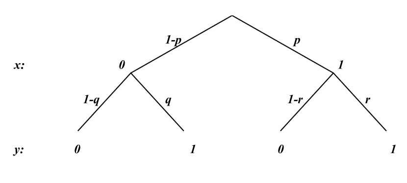
Figure 2.1: A simple decision tree where potentially independent or correlated variables $x$ and $y$ take values $\{0,1\}$ with the probabilities shown. This defines the $(p,q,r)$ behavioural probability space.

2.2 Mixed and behavioural strategy spaces

The different approaches of probability theory and game theory to isomorphic embeddings impacts on the definitions of mixed and behavioural strategy spaces. As previously, we will compare these spaces both with and without isomorphism constraints. Our focus will be on a simple decision problem involving two random variables $x,y\in\{0,1\}$ where $y$ is potentially conditioned on $x$ as shown in the behavioural strategy decision tree of Fig. 2.1.

2.2.1 Mixed strategy space ${\cal P}_{M}$

The mixed strategy space is denoted ${\cal P}_{M}$, and determines the choice of $x$ via a probability distribution $\alpha$ while the respective choices of $y$ on the left branch of the decision tree $y_{l}$ and on the right branch $y_{r}$ are determined by an independent probability distribution $\beta$ according to the following table:

$$\begin{array}[]{c|cccc}(y_{l},y_{r})=&(0,0)&(0,1)&(1,0)&(1,1)\\ \hline\cr(x,y)&\beta_{0}&\beta_{1}&\beta_{2}&\beta_{3}\\ \hline\cr\alpha_{0}&(0,0)&(0,0)&(0,1)&(0,1)\\ \alpha_{1}&(1,0)&(1,1)&(1,0)&(1,1).\\ \end{array}$$ (2.1)

The mixed strategy simplex for each player is respectively $S^{X}=\{(\alpha_{0},\alpha_{1})\in R_{+}^{2}:\sum_{j}\alpha_{j}=1\}$ and $S^{Y}=\{(\beta_{0},\beta_{1},\beta_{2},\beta_{3})\in R_{+}^{4}:\sum_{j}\beta_{j}=1\}$. The associated tangent spaces are $T^{X}=\{z\in R^{2}:\sum_{j}z_{j}=0\}$ and $T^{Y}=\{z\in R^{4}:\sum_{j}z_{j}=0\}$, equivalent to every possible positive or negative fluctuation in the probabilities of the pure strategies of each player. The joint probability distribution $P_{xy}(x,y)$ for $x$ and $y$ is

$$P_{xy}(0,0) = (1-\alpha_{1})(1-\beta_{2}-\beta_{3})$$

$$P_{xy}(0,1) = (1-\alpha_{1})(\beta_{2}+\beta_{3})$$

$$P_{xy}(1,0) = \alpha_{1}(1-\beta_{1}-\beta_{3})$$

$$P_{xy}(1,1) = \alpha_{1}(\beta_{1}+\beta_{3}).$$ (2.2)

Here, we have used normalization constraints to eliminate $\alpha_{0}$ and $\beta_{0}$. The expectations of the $x$ and $y$ variables are given by

$$\langle x\rangle = \alpha_{1}$$

$$\langle y\rangle = \beta_{2}+\beta_{3}+\alpha_{1}(\beta_{1}-\beta_{2})$$

$$\langle xy\rangle = \alpha_{1}(\beta_{1}+\beta_{3}),$$ (2.3)

while their variances are

$$V(x) = \alpha_{1}(1-\alpha_{1})$$

$$V(y) = \left[\beta_{2}+\beta_{3}+\alpha_{1}(\beta_{1}-\beta_{2})\right]\times\left[1-\beta_{2}-\beta_{3}-\alpha_{1}(\beta_{1}-\beta_{2})\right].$$ (2.4)

For completeness, we note the marginal and joint entropies are

$$E_{x} = -(1-\alpha_{1})\log(1-\alpha_{1})-\alpha_{1}\log\alpha_{1}$$

$$E_{y} = -[1-\beta_{2}-\beta_{3}+\alpha_{1}(\beta_{2}-\beta_{1})]\times\log[1-\beta_{2}-\beta_{3}+\alpha_{1}(\beta_{2}-\beta_{1})]$$

$$-[\beta_{2}+\beta_{3}-\alpha_{1}(\beta_{2}-\beta_{1})]\times\log[\beta_{2}+\beta_{3}-\alpha_{1}(\beta_{2}-\beta_{1})]$$

$$E_{xy} = -(1-\alpha_{1})(1-\beta_{2}-\beta_{3})\log[(1-\alpha_{1})(1-\beta_{2}-\beta_{3})]$$ (2.5)

$$-(1-\alpha_{1})(\beta_{2}+\beta_{3})\log[(1-\alpha_{1})(\beta_{2}+\beta_{3})]$$

$$-\alpha_{1}(1-\beta_{1}-\beta_{3})\log[\alpha_{1}(1-\beta_{1}-\beta_{3})]$$

$$-\alpha_{1}(\beta_{1}+\beta_{3})\log[\alpha_{1}(\beta_{1}+\beta_{3})].$$

Naturally, the mixed strategy probability space can model any state of correlation between $x$ and $y$ with the correlation give by

$$\rho_{xy}(\alpha_{1},\beta_{1},\beta_{2},\beta_{3})=\frac{\sqrt{\alpha_{1}(1-\alpha_{1})}(\beta_{1}-\beta_{2})}{\sqrt{\langle y\rangle\left[1-\langle y\rangle\right]}}.$$ (2.6)

Then, when $x$ and $y$ are perfectly correlated we have $\rho_{xy}=1$ requiring the constraints $\beta_{1}=1$ and $\beta_{0}=\beta_{2}=\beta_{3}=0$. When $x$ and $y$ are perfectly anti-correlated we have $\rho_{xy}=-1$ requiring the constraints $\beta_{2}=1$ and $\beta_{0}=\beta_{1}=\beta_{3}=0$. Finally, when $x$ and $y$ are independent we have $\rho_{xy}=0$ requiring the constraint $\beta_{1}=\beta_{2}$.

2.2.2 Behavioural strategy space ${\cal P}_{B}$

The behavioural strategy probability space [4] is denoted ${\cal P}_{B}$ and is parameterized as shown in Fig. 2.1. The behavioural strategy space for the players is $S^{XY}=\{(p,q,r)\in R_{+}^{3}:0\leq p,q,r\leq 1\}$ after taking account of normalization. The associated tangent space is $T^{XY}=\{z\in R^{3}\}$. The probability $P_{xy}(x,y)$ that $x$ and $y$ take on their respective values is

$$P_{xy}(0,0) = (1-p)(1-q)$$

$$P_{xy}(0,1) = (1-p)q$$

$$P_{xy}(1,0) = p(1-r)$$

$$P_{xy}(1,1) = pr.$$ (2.7)

This distribution gives the following expected values:

$$\langle x\rangle = p$$

$$\langle y\rangle = q+p(r-q)$$

$$\langle xy\rangle = pr,$$ (2.8)

while the variances of the $x$ and $y$ variables are

$$V(x) = p(1-p)$$

$$V(y) = \left[q+p(r-q)\right]\left[1-q-p(r-q)\right].$$ (2.9)

The marginal and joint entropies between the $x$ and $y$ variables are

$$E_{x} = -(1-p)\log(1-p)-p\log p$$

$$E_{y} = -[(1-p)(1-q)+p(1-r)]\times\log[(1-p)(1-q)+p(1-r)]$$

$$-[(1-p)q+pr]\log[(1-p)q+pr]$$

$$E_{xy} = -(1-p)(1-q)\log[(1-p)(1-q)]-(1-p)q\log[(1-p)q]$$ (2.10)

$$-p(1-r)\log[p(1-r)]-pr\log[pr].$$

The behavioural probability space also allows modeling any arbitrary state of correlation between the $x$ and $y$ variables where the correlation between $x$ and $y$ is

$$\rho_{xy}=\frac{\sqrt{p(1-p)}(r-q)}{\sqrt{\left[q+p(r-q)\right]\left[1-q-p(r-q)\right]}}.$$ (2.11)

Then, $x$ and $y$ are perfectly correlated at $\rho_{xy}(p,0,1)=1$, perfectly anti-correlated at $\rho_{xy}(p,1,0)=-1$, and uncorrelated if either $p=0$ or $p=1$ or $q=r$ giving $\rho_{xy}=0$. Hence, the decision tree of Fig. 2.1 encompasses every possible state of correlation between $x$ and $y$, and thus it can be used to perform a complete analysis.

$\rho_{xy}=1$	${\cal P}_{M}$	${\cal P}_{B}$	$\left.{\cal P}_{M}\right|_{\beta_{1}=1}$	$\left.{\cal P}_{B}\right|_{(q,r)=(0,1)}$
Parameters	$\alpha_{1},\beta_{1},\beta_{2},\beta_{3}$	$p,q,r$	$\alpha_{1}$	$p$
Dimensions	4	3	1	1
$\nabla$ operator	$\frac{\partial}{\partial\alpha_{1}}\hat{\alpha}_{1}+\frac{\partial}{\partial\beta 1}\hat{\beta}_{1}+\frac{\partial}{\partial\beta_{2}}\hat{\beta}_{2}+\frac{\partial}{\partial\beta_{3}}\hat{\beta}_{3}$	$\frac{\partial}{\partial p}\hat{p}+\frac{\partial}{\partial q}\hat{q}+\frac{\partial}{\partial r}\hat{r}$	$\frac{\partial}{\partial\alpha_{1}}\hat{\alpha}_{1}$	$\frac{\partial}{\partial p}\hat{p}$
Gradient	$\lim_{\beta_{1}\rightarrow 1}\nabla(.)$	$\lim_{(q,r)\rightarrow(0,1)}\nabla(.)$	$\nabla$	$\nabla$
Probability Conservation
$\nabla\left[P_{xy}(0,0)+P_{xy}(1,1)\right]$	$\alpha_{1}\hat{\beta}_{1}-(1-\alpha_{1})\hat{\beta}_{2}+(2\alpha_{1}-1)\hat{\beta}_{3}$	$-(1-p)\hat{q}+p\hat{r}$	0	0
$\nabla\left[P_{xy}(0,1)+P_{xy}(1,0)\right]$	$-\alpha_{1}\hat{\beta}_{1}+(1-\alpha_{1})\hat{\beta}_{2}-(2\alpha_{1}-1)\hat{\beta}_{3}$	$(1-p)\hat{q}-p\hat{r}$	0	0
Conditionals
$\nabla P_{x|y}(0|0)$	$\frac{\alpha_{1}}{1-\alpha_{1}}(\hat{\beta}_{1}+\hat{\beta}_{3})$	$\frac{p}{1-p}\hat{r}$	0	0
$\nabla P_{x|y}(0|1)$	$\frac{1-\alpha_{1}}{1\alpha_{1}}(\hat{\beta}_{2}+\hat{\beta}_{3})$	$\frac{1-p}{p}\hat{q}$	0	0
Expectations
$\nabla\langle x\rangle$	$\hat{\alpha}_{1}$	$\hat{p}$	$\hat{\alpha}_{1}$	$\hat{p}$
$\nabla\langle y\rangle$	$\hat{\alpha}_{1}+\alpha_{1}\hat{\beta}_{1}+(1-\alpha_{1})\hat{\beta}_{2}+\hat{\beta}_{3}$	$\hat{p}+(1-p)\hat{q}+p\hat{r}$	$\hat{\alpha}_{1}$	$\hat{p}$
$\nabla\langle xy\rangle$	$\hat{\alpha}_{1}+\alpha_{1}\hat{\beta}_{1}+\alpha_{1}\hat{\beta}_{3}$	$\hat{p}+p\hat{r}$	$\hat{\alpha}_{1}$	$\hat{p}$
Variance
$\nabla\left[V(x)+V(y)-2\mbox{cov}(x,y)\right]$	$-\alpha_{1}\hat{\beta}_{1}+(1-\alpha_{1})\hat{\beta}_{2}+(1-2\alpha_{1})\hat{\beta}_{3}$	$(1-p)\hat{q}-p\hat{r}$	0	0
Entropy
$\nabla\left[E_{xy}-E_{x}\right]$	$\neq 0$	$\neq 0$	0	0
Correlation
$\nabla\rho_{xy}$	$\neq 0$	$\neq 0$	0	0
$\rho_{xy}=0$	${\cal P}_{M}$	${\cal P}_{B}$	$\left.{\cal P}_{M}\right|_{\beta_{1}=\beta_{2}}$	$\left.{\cal P}_{B}\right|_{r=q}$
Parameters	$\alpha_{1},\beta_{1},\beta_{2},\beta_{3}$	$p,q,r$	$\alpha_{1}$, $\bar{\beta}=\beta_{1}+\beta_{3}$	$p,q$
Dimensions	4	3	2	2
$\nabla$ operator	$\frac{\partial}{\partial\alpha_{1}}\hat{\alpha}_{1}+\frac{\partial}{\partial\beta 1}\hat{\beta}_{1}+\frac{\partial}{\partial\beta_{2}}\hat{\beta}_{2}+\frac{\partial}{\partial\beta_{3}}\hat{\beta}_{3}$	$\frac{\partial}{\partial p}\hat{p}+\frac{\partial}{\partial q}\hat{q}+\frac{\partial}{\partial r}\hat{r}$	$\frac{\partial}{\partial\alpha_{1}}\hat{\alpha}_{1}+\frac{\partial}{\partial\bar{\beta}}\hat{\bar{\beta}}$	$\frac{\partial}{\partial p}\hat{p}+\frac{\partial}{\partial q}\hat{q}$
Gradient	$\lim_{\beta_{2}\rightarrow\beta_{1}}\nabla(.)$	$\lim_{r\rightarrow q}\nabla(.)$	$\nabla$	$\nabla$
Probability
$\nabla\left[P_{xy}(0,0)-P_{x}(0)P_{y}(0)\right]$	$\alpha_{1}(1-\alpha_{1})(\hat{\beta}_{1}-\hat{\beta}_{2})$	$p(1-p)(\hat{r}-\hat{q})$	0	0
$\nabla\left[P_{xy}(0,1)-P_{x}(0)P_{y}(1)\right]$	$\alpha_{1}(1-\alpha_{1})(\hat{\beta}_{2}-\hat{\beta}_{1})$	$p(1-p)(\hat{q}-\hat{r})$	0	0
$\nabla\left[P_{xy}(1,0)-P_{x}(1)P_{y}(0)\right]$	$\alpha_{1}(1-\alpha_{1})(\hat{\beta}_{2}-\hat{\beta}_{1})$	$p(1-p)(\hat{q}-\hat{r})$	0	0
$\nabla\left[P_{xy}(1,1)-P_{x}(1)P_{y}(1)\right]$	$\alpha_{1}(1-\alpha_{1})(\hat{\beta}_{1}-\hat{\beta}_{2})$	$p(1-p)(\hat{r}-\hat{q})$	0	0
Conditionals
$\nabla\left[P_{x|y}(0|0)-P_{x}(0)\right]$	$\frac{\alpha_{1}(1-\alpha_{1})}{1-\beta_{1}-\beta_{3}}(\hat{\beta}_{1}-\hat{\beta}_{2})$	$\frac{p(1-p)}{(1-q)}(\hat{r}-\hat{q})$	0	0
$\nabla\left[P_{x|y}(0|1)-P_{x}(0)\right]$	$\frac{\alpha_{1}(1-\alpha_{1})}{\beta_{1}+\beta_{3}}(\hat{\beta}_{2}-\hat{\beta}_{1})$	$\frac{p(1-p)}{q}(\hat{q}-\hat{r})$	0	0
Expectation
$\nabla\left[\langle xy\rangle-\langle x\rangle\langle y\rangle\right]$	$\alpha_{1}(1-\alpha_{1})(\hat{\beta}_{1}-\hat{\beta}_{2})$	$p(1-p)(\hat{r}-\hat{q})$	0	0
Entropy
$\nabla\left[E_{xy}-E_{x}-E_{y}\right]$	$\neq 0$	$\neq 0$	0	0
Correlation
$\nabla\rho_{xy}$	$\neq 0$	$\neq 0$	0	0

Table 2.1: A comparison of calculated results for mixed ${\cal P}_{M}$ and behavioural ${\cal P}_{B}$ strategy spaces with those same spaces when subject to isomorphic constraints. We examine points where respectively the $x$ and $y$ variables are first perfectly correlated with $\rho_{xy}=1$ and then independent with $\rho_{xy}=1$. In the unconstrained behavioural spaces, all quantities are evaluated at points satisfying $\lim_{\beta_{1}\rightarrow 1}$ or $\lim_{(q,r)\rightarrow(0,1)}$ when $\rho_{xy}=1$, and at points satisfying $\lim_{\beta_{2}\rightarrow\beta_{1}}$ or $\lim_{r\rightarrow q}$ when $\rho_{xy}=0$. The isomorphically constrained spaces are respectively indicated by $\left.{\cal P}_{M}\right|_{\beta_{1}=1}$ and $\left.{\cal P}_{B}\right|_{(q,r)=(0,1)}$ for the perfectly correlated case, and $\left.{\cal P}_{M}\right|_{\beta_{1}=\beta_{2}}$ and $\left.{\cal P}_{B}\right|_{r=q}$ when the variables are independent. Game theory and probability theory assign different dimensionality and tangent spaces to these cases. Many calculated results differ between these spaces.

2.2.3 Isomorphic Mixed and Behavioural Spaces

The mixed ${\cal P}_{M}$ and behavioural ${\cal P}_{B}$ strategy spaces contain embedded probability spaces where $x$ and $y$ are respectively perfectly correlated, independent, or partially correlated. As previously, we will now perform a comparison of probability spaces, both with and without isomorphic constraints, for various correlation states between the $x$ and $y$ variables. That is, we will compare the mixed strategy space ${\cal P}_{M}$ and behavioural strategy space ${\cal P}_{B}$ with isomorphically constrained mixed and behavioural strategy spaces as indicated using the following notation.

The case of perfectly correlated $x$ and $y$ variables is modeled by the spaces

$$\begin{array}[]{ll}\lim_{\beta_{1}\rightarrow 1}{\cal P}_{M}&{\rm mixed}\\ \left.{\cal P}_{M}\right|_{\beta_{1}=1}&{\rm constrained\;mixed}\\ \lim_{(q,r)\rightarrow(0,1)}{\cal P}_{M}&{\rm behavioural}\\ \left.{\cal P}_{B}\right|_{(q,r)=(0,1)}&{\rm constrained\;behavioural}\\ \end{array}$$ (2.12)

In these spaces we expect all of the following to hold:

• $\nabla\left[P_{xy}(0,0)+P_{xy}(1,1)\right]=0$,

• $\nabla\left[P_{xy}(0,1)+P_{xy}(1,0)\right]=0$,

• $\nabla\left[P_{x|y}(0|0)\right]=0$,

• $\nabla\left[P_{x|y}(0|1)\right]=0$,

• $\nabla\left[\langle x\rangle-\langle y\rangle\right]=0$

• $\nabla\left[\langle x\rangle-\langle xy\rangle\right]=0$

• $\nabla\left[\langle y\rangle-\langle xy\rangle\right]=0$

• $\nabla[V(x-y)]=\nabla\left[V(x)+V(y)-2\mbox{cov}(x,y)\right]=0$

• $\nabla\left[E_{xy}-E_{x}\right]=0$.

Alternately, when $x$ and $y$ are independent, the relevant spaces are

$$\begin{array}[]{ll}\lim_{\beta_{1}\rightarrow\beta_{2}}{\cal P}_{M}&{\rm mixed}\\ \left.{\cal P}_{M}\right|_{\beta_{1}=\beta_{2}}&{\rm constrained\;mixed}\\ \lim_{r\rightarrow q}{\cal P}_{M}&{\rm behavioural}\\ \left.{\cal P}_{B}\right|_{r=q}&{\rm constrained\;behavioural}\\ \end{array}$$ (2.13)

In all these spaces, the probability distributions satisfy

• $\nabla\left[P_{xy}-P_{x}P_{y}\right]=0$

• $\nabla\left[P_{x|y}-P_{x}\right]=0$

• $\nabla\left[\langle xy\rangle-\langle x\rangle\langle y\rangle\right]=0$

• $\nabla\left[E_{xy}-E_{x}-E_{y}\right]=0$.

Table 2.1 records whether each of the expected relations is satisfied for each of the mixed and behavioural spaces when they are either unconstrained, or isomorphically constrained. As might be expected, the results indicate that the weak isomorphisms used to construct the mixed and behavioural spaces of game theory are not able to reproduce necessarily true results from probability theory. Hence, the rational player of game theory is unable to reliably reproduce results from probability theory. These differences between game theory and probability theory need to be resolved.

2.3 Discussion

The question posed in this chapter is whether a physical situation involving variables $(x,y)$ defines a set of moves $(x,y)\in\{(0,0),(0,1),(1,0),(1,1)\}$ which then defines a mixed strategy space of three dimensions, or whether the variables $(x,y)$ can be modeled by multiple distinct probability distributions (perfectly correlated, independent, anti-correlated, etc) each of which defines a set of possible moves and corresponding mixed strategy space. These two different approaches can each by modeled using a single mixed strategy space with or without isomorphism constraints. In this case, the question is whether the simple physical decision or game involving the variables $(x,y)$ is best modeled by a single probability space which contains all others without using isomorphic constraints and alters the properties of those embedded spaces to reflect decision uncertainty, or by a single probability space using isomorphic constraints to perfectly preserve the properties of all embedded spaces.

Chapter 3 A simple decision tree optimization

3.1 Optimizing simple decision trees

We now turn to consider how the differences between probability theory and game theory influence decision tree optimization. We consider the usual two potentially correlated random variables depicted in Fig. 2.1 and will use both the unconstrained behavioural probability space ${\cal P}_{B}$ and the isomorphically constrained behavioural spaces $\left.{\cal P}_{B}\right|_{\rho_{xy}=\rho}$ for every value of the correlation state $\rho\in[-1,1]$. Our goal is to present an optimization problem in which a rational player following the rules of game theory cannot achieve the payoff outcomes of a player following the rules of probability theory. We suppose that a player gains a payoff by advising a referee of the parameters of the decision tree probability space $(p,q,r)$ to optimize a given nonlinear random function. The referee uses these parameters to determine the value of the function and provides a payoff equivalent to this value. (If desired, the referee could estimate the probability parameters by using indicator functions and observing an ensemble average of decision tree outcomes.)

3.1.1 Non-polylinear payoff functions

There are many possible random functions which we could use, and some are listed in Table 2.1. We could choose any relations from this table of the form $f=0$ provided probability theory shows $\nabla f=0$ and game theory has $\nabla f\neq 0$. When this is so, the function $\nabla f$ acts effectively as a discrepancy vector. We focus on the squared magnitude of the length of the discrepancy vector and examine functions of the form $F=1-|\nabla f|^{2}$. Immediately, probability theory will optimize this function at the point $F=1$ while game theory will locate an optimum at $F<1$. In particular, we choose

$$f=P_{xy}(0,0)+P_{xy}(0,0)$$ (3.1)

so

$$F = 1-\big{|}\nabla\left[P_{xy}(0,0)+P_{xy}(0,0)\right]\big{|}^{2}$$ (3.2)

$$= 1-\big{|}\nabla\left[1-q+p(q+r-1)\right]\big{|}^{2}.$$

In the unconstrained behavioural space ${\cal P}_{B}$, a rational player will evaluate this as

$$F=1-(1-q-r)^{2}-(1-p)^{2}-p^{2}.$$ (3.3)

In turn, this will be maximized at points $p=\frac{1}{2}$ and $q+r=1$ to give a maximum payoff of $F_{\rm max}=\frac{1}{2}$.

A contrasting result is obtained using the isomorphism constraints of probability theory where our player faces the optimization problem

$$\max F = 1-\big{|}\nabla\left[1-q+p(q+r-1)\right]\big{|}^{2}$$ (3.4)

$$\mbox{ subject to }\rho_{xy}=\rho,\;\;\forall\rho\in[-1,1].$$

Our player might commence by adopting the constraint $\rho_{xy}=1$ implemented by $(q,r)=(0,1)$ to give

$$\max F = \left.1-\big{|}\nabla\left[1-q+p(q+r-1)\right]\big{|}^{2}\right|_{(q,r)=(0,1)}$$ (3.5)

$$= 1.$$

This analysis leads to an optimum point at arbitrary $p$ and $(q,r)=(0,1)$ and a maximum payoff of $F_{\rm max}=1$. Self-evidently, the player would cease their optimization analysis at this point as the achieved maximum can’t be improved.

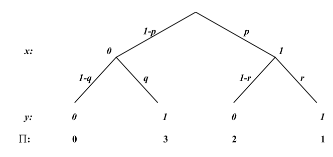
Figure 3.1: A non-strategic decision tree over two stages where a variable $x\in\{0,1\}$ is chosen in the first stage to condition the choice of a second variable $y\in\{0,1\}$ in the second stage. The attained payoffs $\Pi$ are as shown.

3.1.2 Polylinear payoff functions

Of course, there are many random functions defined over decision trees which produce identical results when using or not using isomorphic constraints. We now briefly illustrate this using polylinear expected payoff functions, and consider optimizing the function

$$\max\langle\Pi\rangle = 2\langle x\rangle+3\langle y\rangle-4\langle xy\rangle.$$ (3.6)

$$\mbox{ subject to }\rho_{xy}=\rho,\;\;\forall\rho\in[-1,1]$$

over the decision tree of Fig. 3.1. Of course, simple inspection will locate the optimum at $(\langle x\rangle,\langle y\rangle)=(0,1)$ giving an expected payoff of $\langle\Pi\rangle=3$. However, we step through the process for later generalization to strategic games.

Figure 3.2: The decision tree resulting when the variables $x$ and $y$ are perfectly correlated.

There are an infinite number of correlation constraints to be examined, but several are straightforward. As shown in Fig. 3.2, when the variables are perfectly correlated at $\rho_{xy}=1$ via the constraint $(q,r)=(0,1)$, we have $\langle x\rangle=\langle y\rangle=\langle xy\rangle$ giving

$$\langle\Pi\rangle=\langle x\rangle.$$ (3.7)

This is optimized by setting $\langle x\rangle=1$ giving an expected payoff of $\langle\Pi\rangle=1$.

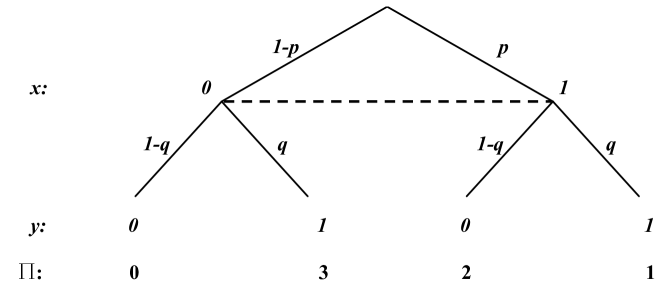
Figure 3.3: The decision tree resulting when the variables $x$ and $y$ are independent.

Fig. 3.3 sets $\rho_{xy}=0$ so the $x$ and $y$ variables are independent by using the constraint $r=q$. The expectations are now separable giving $\langle xy\rangle=\langle x\rangle\langle y\rangle$ and

$$\langle\Pi\rangle=2\langle x\rangle+3\langle y\rangle-4\langle x\rangle\langle y\rangle.$$ (3.8)

As the $\langle x\rangle$ and $\langle y\rangle$ variables are independent, a check of internal stationary points and the boundary leads to an optimal point at $(\langle x\rangle,\langle y\rangle)=(0,1)$ and an expected payoff of $\langle\Pi\rangle=3$.

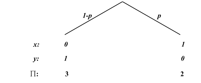
Figure 3.4: The decision tree resulting when the variables $x$ and $y$ are perfectly anti-correlated.

We lastly consider the case where the variables are perfectly anti-correlated. As shown in Fig. 3.4, when the variables are perfectly correlated at $\rho_{xy}=-1$ via the constraint $(q,r)=(1,0)$, we have $\langle y\rangle=(1-\langle x\rangle)$ and $\langle xy\rangle=0$ giving

$$\langle\Pi\rangle=3-\langle x\rangle.$$ (3.9)

This is optimized by setting $\langle x\rangle=0$ giving an expected payoff of $\langle\Pi\rangle=3$.

More general correlation states require use of, for instance, standard Lagrangian optimization procedures.

However, we here adopt a numerical optimization approach by first using the correlation constraint to write the $r$ variable as a function of $p$, $q$ and the correlation constant $\rho$, giving a function $r=r_{+}(p,q,\rho)$. In particular, when the correlation (Eq. 2.11) between $x$ and $y$ is $\rho_{xy}=\rho$, and as long as both $p\neq 0$ and $p\neq 1$, then the correlation constraint defines two surfaces in the $(p,q,r)$ simplex at height

$$r_{\pm}(p,q,\rho)=\frac{\rho^{2}-2q(1-p)(\rho^{2}-1)\pm\rho\sqrt{\rho^{2}+4q(1-q)\frac{(1-p)}{p}}}{2\left[1+p(\rho^{2}-1)\right]}.$$ (3.10)

The function $r_{+}(p,q,\rho)$ will give the correlation surfaces we require within the simplex. That is, when $\rho=0$ we have $r_{+}(p,q,0)=q$ as required. Similarly, when $\rho=1$ we have $r_{+}(p,q,1)\geq 1$ across the entire $(p,q)$ plane with the equality $r_{+}(p,q,1)=1$ only where $q=0$ or $q=1$. We require $\rho=1$ at $(q,r)=(0,1)$. Finally, when $\rho=-1$ and $x$ and $y$ are perfectly anti-correlated, we have $r_{+}(p,q,-1)\leq 0$ across the entire $(p,q)$ plane with the equality $r_{+}(p,q,-1)=0$ only where $q=0$ or $q=1$. We require $\rho=-1$ at $(q,r)=(1,0)$.

The strict requirement that $0\leq r_{+}(p,q,\rho)\leq 1$ establishes permissible regions on the $(p,q)$ plane. For $0<\rho<1$, the permissible region is bounded by the $q=0$ line and the line

$$q(p,\rho)=\frac{p}{p+\frac{\rho^{2}}{1-\rho^{2}}}.$$ (3.11)

Similarly, for $-1<\rho<0$, the $(p,q)$ region is bounded by the $q=1$ line and the line

$$q(p,\rho)=\frac{1}{1+p\frac{1-\rho^{2}}{\rho^{2}}}.$$ (3.12)

The problem is then solved using a a typical Mathematica command line of [22]

$$\mbox{NMaximize}[\{\mbox{inRange}[r_{+}(p,q,\rho)]\times\left[2p+3q-3pq-pr_{+}(p,q,\rho)\right],$$

$$0\leq p\leq 1\mbox{ \&\& }0\leq q\leq 1\},\{p,q\}].$$ (3.13)

Here, a suitably defined “inRange” function determines whether $r_{+}$ is taking permissible values between zero and unity allowing the payoff function to be examined over the entire $(p,q)$ plane. The resulting optimal expected payoffs are follows:

$$\begin{array}[]{l|l|l|l}\rho&(p,q,r)&\langle\Pi\rangle\\ \hline\cr+1&(1.,0.,1.)&1.\\ +0.75&(0.8138,0.3876,1.)&1.03032\\ +0.5&(0.4831,0.5917,1.)&1.40068\\ +0.25&(0.2590,0.7953,1.)&2.02693\\ 0&(0.,1.,1.)&3.\\ -0.25&(0.,1.,0.9378)&3.\\ -0.5&(0.,1.,0.7506)&3.\\ -0.75&(0.,1.,0.4386)&3.\\ -1&(0.,1.,0.)&3.\\ \end{array}$$ (3.14)

Some care must be taken to ensure convergence of the solution. This analysis makes it evident that the player can maximize expected payoffs by choosing a correlation constraint where $x$ and $y$ is independent (say) allowing the setting $(p,q,r)=(0,1,1)$ to gain a payoff of $\langle\Pi\rangle=3$. Other choices would also have been possible.

We now turn to applying isomorphism constraints to the strategic analysis of game theory.

Chapter 4 A simple two-player-two-stage optimization

4.1 Optimizing a multistage game tree

In this section, we show that the use of isomorphic constraints can alter the outcomes of strategic games even when expected payoff functions are being used. We will consider either the mixed strategy space ${\cal P}_{M}$ (Eq. 2.2.1) and the behavioural strategy space ${\cal P}_{B}$ (Eq. 2.2.2) or the isomorphically constrained behavioural spaces $\left.{\cal P}_{B}\right|_{\rho_{xy}=\rho}$ for every value of the correlation state $\rho\in[-1,1]$.

We consider a strategic interaction between two players over multiple stages as depicted in Fig. 4.1. Here, two players denoted $X$ and $Y$ seek to optimize their respective payoffs

$$X:\max\Pi^{X}(x,y) = 3-2x-y+4xy$$

$$Y:\max\Pi^{Y}(x,y) = 1+3x+y-2xy.$$ (4.1)

Again, we assume a domain $x,y\in\{0,1\}$ and that player $X$ chooses the value of $x$ and advises this to $Y$ before $Y$ determines the value of $y$. Players will either consider the payoff functions above or their expectations

$$X:\max\langle\Pi^{X}\rangle = 3-2\langle x\rangle-\langle y\rangle+4\langle xy\rangle$$

$$Y:\max\langle\Pi^{Y}\rangle = 1+3\langle x\rangle+\langle y\rangle-2\langle xy\rangle.$$ (4.2)

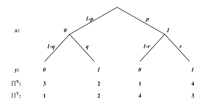
Figure 4.1: Two players, $X$ and $Y$ conduct a two-stage sequential game where $X$ chooses the first variable $x\in\{0,1\}$ and $Y$ chooses the second variable $y\in\{0,1\}$ conditioned on $x$. The payoffs for players are $\Pi^{X}$ and $\Pi^{Y}$.

4.1.1 Unconstrained mixed space ${\cal P}_{M}$

For the unconstrained mixed strategy space ${\cal P}_{M}$, the expected payoffs for each player are

$$\begin{array}[]{c|cccc}(y_{l},y_{r})=&(0,0)&(0,1)&(1,0)&(1,1)\\ \hline\cr(\langle\Pi^{X}\rangle,\langle\Pi^{Y}\rangle)&\beta_{0}&\beta_{1}&\beta_{2}&\beta_{3}\\ \hline\cr\alpha_{0}&(3,1)&(3,1)&(2,2)&(2,2)\\ \alpha_{1}&(1,4)&(4,3)&(1,4)&(4,3).\\ \end{array}$$ (4.3)

Using this table, the expected payoff functions take the form

$$\langle\Pi^{X}\rangle = 3-\beta_{2}-\beta_{3}+\alpha_{1}(-2+3\beta_{1}+\beta_{2}+4\beta_{3})$$

$$\langle\Pi^{Y}\rangle = 1+\beta_{2}+\beta_{3}+\alpha_{1}(3-\beta_{1}-\beta_{2}-2\beta_{3})$$ (4.4)

while the unconstrained gradients evaluate as

$$\nabla\langle\Pi^{X}\rangle = (-2+3\beta_{1}+\beta_{2}+4\beta_{3})\hat{\alpha}_{1}+3\alpha_{1}\hat{\beta}_{1}+(\alpha_{1}-1)\hat{\beta}_{2}+(4\alpha_{1}-1)\hat{\beta}_{3}$$

$$\nabla\langle\Pi^{Y}\rangle = (3-\beta_{1}-\beta_{2}-2\beta_{3})\hat{\alpha}_{1}-\alpha_{1}\hat{\beta}_{1}+(1-\alpha_{1})\hat{\beta}_{2}+(1-2\alpha_{1})\hat{\beta}_{3}.$$ (4.5)

The expected payoff can then optimized by either comparing returns in the payoff table for each mixed strategy combination, or by the equivalent strategy of comparing the simultaneous rates of change of the payoff functions with the probability parameters. (To illustrate the second approach, the rate of change of $\langle\Pi^{Y}\rangle$ with $\beta_{1}$ is equal to $-\alpha_{1}$ which is almost always negative indicating that payoffs are maximized by setting $\beta_{1}=0$.) Either approach then locates the optimal mixed strategy of $(\alpha_{1},\beta_{1},\beta_{2},\beta_{3})=(0,0,1,0)$ leading to expected payoffs of $(\langle\Pi^{X}\rangle,\langle\Pi^{Y}\rangle)=(2,2)$.

4.1.2 Unconstrained behavioural space ${\cal P}_{B}$

The unconstrained behavioural strategy space ${\cal P}_{B}$ is pictured in Fig. 2.1. The unconstrained optimization problem faced by each player is

$$X:\max_{p}\langle\Pi^{X}\rangle = 3-2p-q+pq+3pr$$

$$Y:\max_{q,r}\langle\Pi^{Y}\rangle = 1+3p+q-pq-pr.$$ (4.6)

The unconstrained gradients of the expected payoffs evaluate as

$$\nabla\langle\Pi^{X}\rangle = (q+3r-2)\hat{p}-(1-p)\hat{q}+3p\hat{r}$$

$$\nabla\langle\Pi^{Y}\rangle = (3-q-r)\hat{p}+(1-p)\hat{q}-p\hat{r}.$$ (4.7)

This perfect information game can then be optimized by inspection, or by equating gradients to zero, or by using backwards induction. The resulting optimal pure strategy choices are $(x,y)=(0,1)$ giving payoffs of $(\Pi^{X},\Pi^{Y})=(2,2)$.

4.1.3 Constrained behavioural space $\left.{\cal P}_{B}\right|_{\rho_{xy}=\rho}$

We now consider the constrained behavioural spaces $\left.{\cal P}_{B}\right|_{\rho_{xy}=\rho},\forall\rho\in[-1,1]$. The two players are non-communicating and it is generally not possible to use a single value for the correlation $\rho$, and this generally makes the analysis intractable. However, player $Y$ has total control over the setting of the correlation $\rho$ in three cases—when $\rho=\pm 1$ and $\rho=0$. We consider these cases now.

First consider the space ${\cal P}_{B}|_{\rho_{xy}=1}$ in which the variables are functionally equal so $y=x=xy$. (We can consider the payoff functions directly rather than their expected values.) In this space the players face the respective optimization tasks

$$X:\max_{x}\Pi^{X}(x) = 3+x$$

$$Y:\Pi^{Y}(x) = 1+2x.$$ (4.8)

As a result, player $X$ optimizes their payoff by setting $x=1$ giving the outcomes $(\Pi^{X},\Pi^{Y})=(4,3)$.

In contrast, in the space ${\cal P}_{B}|_{\rho_{xy}=-1}$, the variables are functionally related by $y=1-x$ and $xy=0$. These constraints render the optimization tasks as

$$X:\max_{x}\Pi^{X}(x) = 2-x$$

$$Y:\Pi^{Y}(x) = 2+2x.$$ (4.9)

Here, player $X$ chooses $x=0$ to optimize their payoff leading to the outcomes $(\Pi^{X},\Pi^{Y})=(2,2)$.

Finally, when player $Y$ chooses to discard all information about the $x$ variable, then the variables $x$ and $y$ are independent and the chosen space is ${\cal P}_{B}|_{\rho_{xy}=0}$. When the variables are independent, there might not necessarily be a pure strategy solution and we need to optimize expected payoffs. In this space, we have $\langle x\rangle=p$ and $\langle y\rangle=q$ and $\langle xy\rangle=\langle x\rangle\langle y\rangle=pq$ giving the optimization problem

$$X:\max_{p}\langle\Pi^{X}\rangle = 3-2p-q+4pq$$

$$Y:\max_{q}\langle\Pi^{Y}\rangle = 1+3p+q-2pq.$$ (4.10)

The best response functions or equivalent partial differentials are

$$X:\frac{\partial\langle\Pi^{X}\rangle}{\partial p} = -2+4q$$

$$Y:\frac{\partial\langle\Pi^{Y}\rangle}{\partial q} = 1-2p$$ (4.11)

locating the optimal point at $(p,q)=(\frac{1}{2},\frac{1}{2})$ with expected payoffs of $(\langle\Pi^{X}\rangle,\langle\Pi^{Y}\rangle)=(\frac{5}{2},\frac{5}{2})$.

At this stage of the analysis, both players have separately calculated an equilibrium point in three spaces ${\cal P}_{B}|_{\rho_{xy}=\rho}$ for $\rho\in\{-1,0,1\}$, and the selection of these correlation states is solely at the discretion of player $Y$. The expected payoffs gained at each of these “local” equilibrium points can then be compared to obtain a “global” optimal expected payoff. For convenience, these are summarized here:

$$\begin{array}[]{cc}\rho&(\langle\Pi^{X}\rangle,\langle\Pi^{Y}\rangle)\\ \hline\cr-1&(2,2)\\ 0&(\frac{5}{2},\frac{5}{2})\\ +1&(4,3).\\ \end{array}$$ (4.12)

Based on these results, player $Y$ will then rationally optimize their expected payoff by choosing to have their variables in a state of perfect correlation with $\rho=1$ in the space ${\cal P}_{B}|_{\rho_{xy}=1}$. Player $X$, also being a rational optimizer will play accordingly to give equilibrium payoffs of $(\langle\Pi^{X}\rangle,\langle\Pi^{Y}\rangle)=(4,3)$.

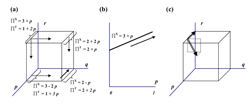
Figure 4.2: (a) Game theory adopts an unconstrained joint probability measure space in which expected payoffs vary over three dimensions $(p,q,r)$ and where positive gradients with respect to $q$ and $r$ (dotted arrows) and with respect to $p$ (solid arrow) ensure that players maximize joint payoffs by choosing $(p,q,r)=(0,1,0)$. (b) An alternate joint probability space where $x$ is perfectly correlated to $y$ in which expected payoffs vary over a single dimension $p$ with positive gradients with respect to $p$ (solid arrow) ensuring that players optimize payoffs by choosing $p=1$. (c) The choice of two alternate probability spaces (more are possible) associates two different total gradients (double-lined arrows) with any point along the perfect correlation line $\rho_{xy}=1$ at $(q,r)=(0,1)$. In the absence of any effective decision procedure privileging any one space over another, players should examine all possible spaces, all possible gradients, and all possible optimized outcomes.

It is useful again to reemphasize a geometric picture. As shown in Fig. 4.2(a), an unconstrained behavioural space has a three-dimensional gradient everywhere which is non-zero even when $x$ and $y$ are perfectly correlated so payoffs are not optimized at any such points. In contrast, the use of isomorphic constraints when the $x$ and $y$ variables are perfectly correlated gives the situation in Fig. 4.2(b) where now a 1-dimensional gradient points solely along the $\hat{p}$ axis. A comparison in Fig. 4.2(c) of the resulting outcomes can then be made to determine which probability space should be chosen so as to maximize outcomes.

4.1.4 Strategic analysis difficulties

The players might then seek to supplement the above solutions by considering a wider range of correlation states.The optimization task then becomes

$$X:\max_{p}\langle\Pi^{X}\rangle = 3-2p-q+pq+3pr$$

$$Y:\max_{q,r}\langle\Pi^{Y}\rangle = 1+3p+q-pq-pr$$ (4.13)

$$\mbox{ subject to }\rho_{xy}=\rho,\;\;\forall\rho\in[-1,1].$$

Unfortunately, there does not seem to be any straightforward way to make progress with the general correlation case. Players are non-communicating and hence cannot agree on a value of the correlation state $\rho$. If players adopt different values of the correlation states they must model conflicting global constraints and it is not clear how these can be resolved. An attempt to model the use of a single correlation state generates expected payoff functions which are not poly-linear in the probability parameters and that are not generally quasi-concave. This implies that existence theorems for Nash equilibria are inapplicable in these cases so equilibrium points might not exist for different correlation states. It is more than likely that an acceptable solution methodology does not exist for strategic interactions in the general correlation case, and it is beyond the scope of this paper to consider this issue further. Here finally, we find the irreducible complexity of strategic analysis expected by von Neumann and Morgenstern.

4.1.5 More general constrained analysis

The choice of variable $y$ is normally modeled as requiring two separate and independent coin tosses—see the behavioural space tree of Fig. 4.1. When $x=0$ a coin is tossed determining $y=u\in\{0,1\}$ with respective probabilities $(1-q,q)$, while when $x=1$ another coin is tossed determining $y=v\in\{0,1\}$ with respective probabilities $(1-r,r)$. The $u$ and $v$ coins are then simple, biassed, independent coins.

However, there is no need for this simplest possible treatment. The $u$ and $v$ coins could themselves be modeled using any of the alternate probability spaces of Eqs. 1.21—1.34. These alternate probability spaces would need to be checked by rational players of unbounded capacity.

Another possible probability space might consider the $u$ and $v$ variables themselves to be partially correlated. That is, the second stage player chooses to partially correlate their two behavioural strategies by employing two sequential roulettes. The first determines the variable $u\in\{0,1\}$ with probabilities $(1-q,q)$ while the second gives $v\in\{0,1\}$ with respective probabilities $(1-r_{1},r_{1})$ if $u=0$ and $(1-r_{2},r_{2})$ if $u=1$. The resulting correlation between the variables $u$ and $v$ is then

$$\rho_{uv}(q,r_{1},r_{2})=\frac{\sqrt{q(1-q)}(r_{2}-r_{1})}{\sqrt{\left[r_{1}+q(r_{2}-r_{1})\right]\left[1-r_{1}-q(r_{2}-r_{1})\right]}}.$$ (4.14)

When $r_{1}=r_{2}$ then these variables are uncorrelated as usual. In turn, this correlation between the $u$ and $v$ variables renders the correlation between the $x$ and $y$ variables as

$$\rho_{xy}(p,q,r_{1},r_{2})=\frac{\sqrt{p(1-p)}[r_{1}-q(1+r_{1}-r_{2})]}{\sqrt{\left[q+p(r_{1}-q)+pq(r_{2}-r_{1})\right]\left[1-q+p(r_{1}-q)+pq(r_{2}-r_{1})\right]}}.$$ (4.15)

The second stage player might then choose to adopt a probability space with a constant correlation between the $u$ and $v$ variables, say $\rho_{uv}(q,r_{1},r_{2})=\bar{\rho}_{uv}$ say. If $\bar{\rho}_{uv}=0$ then we have the usual situation of uncorrelated behavioural strategies normally considered by game theory. Conversely, if $\bar{\rho}_{uv}=\pm 1$ we have respectively either perfectly correlated or perfectly anti-correlated behavioural strategies. If such a correlation constraint can be adopted, then both players should analyze this possibility to determine whether it is optimal.

Even more strangely, the $u$ and $v$ coin tosses could themselves be partially correlated to the previous choice of $x$. That is, the $u$ and $v$ variables can be correlated with $x$, and only after they have been chosen is the value for $y$ assigned. For example, we might have $u$ perfectly anti-correlated with $x$ so $u=1-x$ and $v$ perfectly correlated with $x$ so $v=x$, and then we assign $y=u$ if $x=0$ and $y=v$ if $x=1$. There are many possible choices that might be considered. In particular, we might consider the 9 possible cases which arise when firstly the $u$ variable is either perfectly anti-correlated to $x$ (denoted ${\cal P}^{Y}_{-.}$), independent of $x$ (${\cal P}^{Y}_{0.}$) or perfectly correlated to $x$ (${\cal P}^{Y}_{+.}$), and the $v$ variable is either perfectly anti-correlated to $x$ (denoted ${\cal P}^{Y}_{.-}$), independent of $x$ (${\cal P}^{Y}_{.0}$) or perfectly correlated to $x$ (${\cal P}^{Y}_{.+}$). We have introduced subscript symbols indicating these possibilities. That is, we separately have

$$P^{Y}(u) = \left\{\begin{array}[]{cc}\delta_{u(1-x))}&{\cal P}^{Y}_{-.}\\ &\\ (1-q,q)&{\cal P}^{Y}_{0.}\\ &\\ \delta_{ux}&{\cal P}^{Y}_{+.}\\ \end{array}\right.$$ (4.21)

$$P^{Y}(v) = \left\{\begin{array}[]{cc}\delta_{v(1-x)}&{\cal P}^{Y}_{.-}\\ &\\ (1-r,r)&{\cal P}^{Y}_{.0}\\ &\\ \delta_{vx}&{\cal P}^{Y}_{.+}\\ \end{array}\right..$$ (4.27)

The right hand column here lists the shorthand notation for each adopted strategy. This notation shows that if $u$ is independent of $x$ while $v$ is perfectly correlated to $x$, the second stage probability distribution adopted by player $Y$ is ${\cal P}^{Y}_{0+}$. Similarly, when both $u$ and $v$ are perfectly correlated to $x$ we have the probability distribution ${\cal P}^{Y}_{++}$. Each of these choices of a different probability space generates a different optima within that space, and these optima must be compared so that players can decide which space they can rationally choose. Without showing the details, the generated outcomes in these possible spaces are

$$\begin{array}[]{c|c}&(\langle\Pi^{X}\rangle,\langle\Pi^{Y}\rangle)\\ \hline\cr{\cal P}^{Y}_{--}&(2,2)\\ {\cal P}^{Y}_{-0}&(2,2)\\ {\cal P}^{Y}_{-+}&(4,3)\\ {\cal P}^{Y}_{0-}&(2,2)\\ {\cal P}^{Y}_{00}&(2,2)\\ {\cal P}^{Y}_{0+}&(4,3)\\ {\cal P}^{Y}_{+-}&(3,1)\\ {\cal P}^{Y}_{+0}&(3,1)\\ {\cal P}^{Y}_{++}&(4,3).\\ \end{array}$$ (4.28)

These outcomes can easily be verified by drawing the different trees generated by each choice of joint probability space as shown in Fig. 4.3. This extended table of distinct trees makes evident that again, within this range of considered joint probability spaces, player $Y$ optimizes their outcomes by choosing, for instance, the space ${\cal P}^{Y}_{++}$ ensuring that their choice is perfectly correlated with that of their opponent.

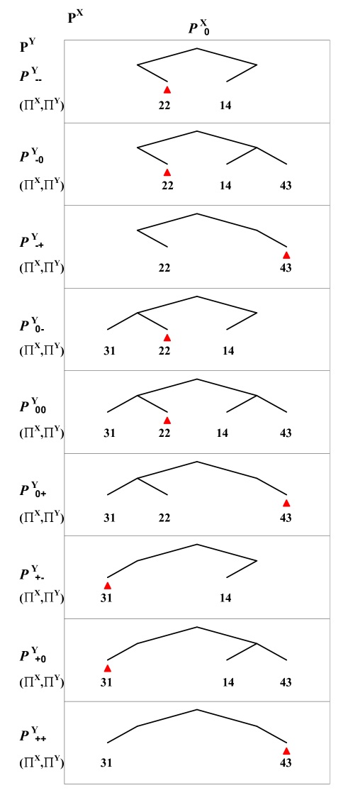
Figure 4.3: The nine distinct trees, payoffs and equilibria (indicated by triangles) given that players $X$ and $Y$ adopt the indicated joint probability space. The two subscript symbols here respectively indicate whether each of player $Y$’s second stage choices are perfectly anti-correlated (“$-$”), uncorrelated (“$0$”), or perfectly correlated (“$+$”) to the previously observed random variable $x$.

We argue that optimizing multiple-player-multiple-stage games is more complicated than envisaged in conventional game analysis. As noted earlier, the strategic optimization of expected payoffs first requires the adoption of a suitable joint probability measure space, and it is only the adoption of such a space that permits the functional definition of both the expected payoff and suitable gradient operators allowing the optimization to be completed. For the above simple two player game, the expected payoffs and gradient operators have been respectively defined variously as

$$\left(\langle\Pi^{X}\rangle,\langle\Pi^{Y}\rangle\right)=\left\{\begin{array}[]{cc}\left(2-p,2+2p\right)&{\cal P}^{Y}_{--}\\ &\\ \left(2-p+3pr,2+2p-pr\right)&{\cal P}^{Y}_{-0}\\ &\\ \left(2+2p,2+p\right)&{\cal P}^{Y}_{-+}\\ &\\ \left(3-2p-q+pq,1+3p+q-pq\right)&{\cal P}^{Y}_{0-}\\ &\\ \left(3-2p-q+pq+3pr,1+3p+q-pq-pr\right)&{\cal P}^{Y}_{00}\\ &\\ \left(3+p-q+pq,1+2p+q-pq\right)&{\cal P}^{Y}_{0+}\\ &\\ \left(3-2p,1+3p\right)&{\cal P}^{Y}_{+-}\\ &\\ \left(3-2p+3pr,1+3p-pr\right)&{\cal P}^{Y}_{+0}\\ &\\ \left(3+p,1+2p\right)&{\cal P}^{Y}_{++}\\ \end{array}\right.$$ (4.29)

and

$$\left[\nabla^{X},\nabla^{Y}\right]=\left\{\begin{array}[]{cc}\left[\left(\frac{\partial}{\partial p}\right),.\right]&{\cal P}^{Y}_{--}\\ &\\ \left[\left(\frac{\partial}{\partial p}\right),\left(\frac{\partial}{\partial r}\right)\right]&{\cal P}^{Y}_{-0}\\ &\\ \left[\left(\frac{\partial}{\partial p}\right),.\right]&{\cal P}^{Y}_{-+}\\ &\\ \left[\left(\frac{\partial}{\partial p}\right),\left(\frac{\partial}{\partial q}\right)\right]&{\cal P}^{Y}_{0-}\\ &\\ \left[\left(\frac{\partial}{\partial p}\right),\left(\frac{\partial}{\partial q},\frac{\partial}{\partial r}\right)\right]&{\cal P}^{Y}_{00}\\ &\\ \left[\left(\frac{\partial}{\partial p}\right),\left(\frac{\partial}{\partial q}\right)\right]&{\cal P}^{Y}_{0+}\\ &\\ \left[\left(\frac{\partial}{\partial p}\right),.\right]&{\cal P}^{Y}_{+-}\\ &\\ \left[\left(\frac{\partial}{\partial p}\right),\left(\frac{\partial}{\partial r}\right)\right]&{\cal P}^{Y}_{+0}\\ &\\ \left[\left(\frac{\partial}{\partial p}\right),.\right]&{\cal P}^{Y}_{++}.\\ \end{array}\right.$$ (4.30)

That is, the expected payoff is defined here as a joint functional mapping from the various probability measure spaces to the reals via

$$\left(\langle\Pi^{X}\rangle,\langle\Pi^{Y}\rangle\right) : \left\{{\cal P}^{X}_{0}\times{\cal P}^{Y}_{--},{\cal P}^{X}_{0}\times{\cal P}^{Y}_{-0},{\cal P}^{X}_{0}\times{\cal P}^{Y}_{-+},{\cal P}^{X}_{0}\times{\cal P}^{Y}_{0-},{\cal P}^{X}_{0}\times{\cal P}^{Y}_{00},\right.$$ (4.31)

$$\left.{\cal P}^{X}_{0}\times{\cal P}^{Y}_{0+},{\cal P}^{X}_{0}\times{\cal P}^{Y}_{+-},{\cal P}^{X}_{0}\times{\cal P}^{Y}_{+0},{\cal P}^{X}_{0}\times{\cal P}^{Y}_{++}\right\}\rightarrow{\rm I\mkern-3.0muR}\times{\rm I\mkern-3.0muR}.$$

Again, this is in sharp contrast to the usual definition of game theory that it is sufficient for optimization to consider that the expected payoff is defined as the joint function mapping

$$\left(\langle\Pi^{X}\rangle,\langle\Pi^{Y}\rangle\right):{\cal P}^{X}_{0}\times{\cal P}^{Y}_{00}\rightarrow{\rm I\mkern-3.0muR}\times{\rm I\mkern-3.0muR}.$$ (4.32)

4.2 Backwards induction and isomorphism constraints

We have mentioned above that backwards induction can be used to solve the unconstrained optimization problem. This approach is often presented as a ‘proof’ that no alternative procedure could possibly be considered by a rational player. It is worth taking a closer look at what is involved in the backwards induction algorithm, and how it interacts with isomorphic constraints.

Backwards induction first constrains the values of first stage probability parameters and then evaluates the gradients of the expected payoff function $\langle\Pi^{Y}\rangle$ at different nodes in the last stage of the game. These last stage gradients are then used to set the optimal values of the $(q,r)$ probability variables. These values are then applied as constraints to the evaluation of the gradient of the expected payoff function $\langle\Pi^{X}\rangle$ in the first stage of the game—the first stage probability parameters are now treated as variables. To illustrate these steps, we choose to begin our analysis at a point in the behavioural strategy space where the variables are perfectly correlated at $(q,r)=(0,1)$. The steps involved are:

$$\lim_{(q,r)\rightarrow(0,1)}\frac{\partial\langle\Pi^{Y}\rangle|_{p=0}}{\partial q} = 1>0,\mbox{ so }q\rightarrow 1$$

$$\lim_{(q,r)\rightarrow(0,1)}\frac{\partial\langle\Pi^{Y}\rangle|_{p=1}}{\partial r} = -1<0,\mbox{ so }r\rightarrow 0$$

$$\left.\frac{\partial\langle\Pi^{X}\rangle}{\partial p}\right|_{(q,r)=(1,0)} = -p<0,\mbox{ so }p\rightarrow 0.$$ (4.33)

The optimal point is then at $(p,q,r)=(0,1,0)$ giving payoffs of $(\langle\Pi^{X}\rangle,\langle\Pi^{Y}\rangle)=(2,2)$.

It is very easy and straightforward to apply the backwards induction algorithm to an isomorphically constrained space, provided that the global isomorphic constraints and the altered geometry is taken into account. If the variables $x$ and $y$ are perfectly correlated then the game tree reduces to a single stage and backwards induction is properly applied to that single stage. However, problems arise when as is common, it is argued that backwards induction must be applied to both stages even when the $x$ and $y$ variables are perfectly correlated. This argument presupposes that backwards induction overrides isomorphic constraints and the altered game geometry.

To see how this is done, let us imagine trying to apply the backwards induction algorithm to an isomorphically constrained perfectly correlated space $\left.{\cal P}_{B}\right|_{(q,r)=(0,1)}$ with $\rho=1$. The above evaluations then try to combine limit processes, gradient evaluations, and isomorphic constraints with global scope. That is:

$$\left.\lim_{(q,r)\rightarrow(0,1)}\frac{\partial\langle\Pi^{Y}\rangle|_{p=0}}{\partial q}\right|_{(q,r)=(0,1)} = ?$$

$$\left.\lim_{(q,r)\rightarrow(0,1)}\frac{\partial\langle\Pi^{Y}\rangle|_{p=1}}{\partial r}\right|_{(q,r)=(0,1)} = ?$$

$$\left.\left.\frac{\partial\langle\Pi^{X}\rangle}{\partial p}\right|_{(q,r)=(0,1)}\right|_{(q,r)=(1,0)} = ?.$$ (4.34)

Mathematically and logically, these statements make little sense. An isomorphic constraint of global scope sets the values $(q,r)=(0,1)$ and then backwards induction seeks to treat these parameters as variables and evaluate a gradient with respect to these variables. In actuality, these variables no longer exist in this constrained probability space as there is no second stage in this probability space. The altered probability space geometry has altered the game try to include only one stage and one probability parameter.

Let us try a slightly more general treatment. Consider briefly the optimization by player $Z\in\{X,Y\}$ of an example two stage game where $x$ is known before $y$ is decided giving

$$\langle\Pi^{Z}\rangle=\sum_{x,y=0}^{1}P^{X}(x)P^{Y}(y|x)\Pi^{Z}(x,y).$$ (4.35)

The conventional analysis begins by drawing a single game tree capturing every possible move that might be made along every history, and assigning independent distributions to each decision point which can then be optimized via backwards induction. Then, backwards induction begins by optimizing the last stage first via, for instance, evaluations like

$$\frac{\partial\langle\Pi^{Z}\rangle}{\partial P^{Y}(y^{\prime}|x^{\prime})} = \frac{\partial}{\partial P^{Y}(y^{\prime}|x^{\prime})}\sum_{x,y=0}^{1}P^{X}(x)P^{Y}(y|x)\Pi^{Z}(x,y)$$ (4.36)

$$= P^{X}(x^{\prime})\frac{\partial}{\partial P^{Y}(y^{\prime}|x^{\prime})}\left[\left(1-P^{Y}(y^{\prime}|x^{\prime})\right)\Pi^{Z}(x^{\prime},1-y^{\prime})+P^{Y}(y^{\prime}|x^{\prime})\Pi^{Z}(x^{\prime},y^{\prime})\right]$$

$$= P^{X}(x^{\prime})\left(\Pi^{Z}(x^{\prime},y^{\prime})-\Pi^{Z}(x^{\prime},1-y^{\prime})\right).$$

Implicit in this evaluation, is the assumption that the gradient operator $\frac{\partial}{\partial P^{Y}(y^{\prime}|x^{\prime})}$ commutes with the distribution $P^{X}(x^{\prime})$ via

$$\frac{\partial}{\partial P^{Y}(y^{\prime}|x^{\prime})}P^{X}(x^{\prime})=P^{X}(x^{\prime})\frac{\partial}{\partial P^{Y}(y^{\prime}|x^{\prime})}.$$ (4.37)

This is only true under the assumption that the distributions $P^{Y}(y|x)$ and $P^{X}(x)$ are not functionally dependent. When this is not the case, then obviously, the above commutation relation cannot be used. Speaking figuratively, for longer $N$ stage games, backwards induction relies on similar independence assumptions allowing gradients with respect to $i^{\rm th}$ stage distributions $P_{i}$ to commute with all earlier stage distributions, giving (loosely)

$$\max_{P_{1},P_{2},\dots,P_{N-1},P_{N}}\langle\Pi^{Z}\rangle=\max_{P_{1}}\;\left[\sum\dots\max_{P_{2}}\;\left[\sum\dots\max_{P_{N-1}}\;\left[\sum\dots\max_{P_{N}}\;\left[\sum\dots\right]\right]\right]\right]$$ (4.38)

Again, commuting latter stage gradient operators through all preceding earlier stage distributions is only valid under the assumption that these distributions are not functionally dependent. These assumptions are not necessarily true, and we suggest that rational players will consider the case where they are not warranted.

In our approach in contrast, we hold that the functionals $\langle\Pi^{Z}\rangle$ cannot be represented by a single game tree of finite size, and that they possess neither dimensionality nor continuity properties. While they are a mapping into a range of reals, their domain sets are essentially unspecified. In fact, and crudely put, if $S$ is the set of all possible feasible spaces for this game, say $S=\{{\rm I\mkern-3.0muR}^{1},{\rm I\mkern-3.0muR}^{2},\dots\}$, then the functional is a mapping from the set of all possible feasible spaces to the reals, $\langle\Pi^{Z}\rangle:S\rightarrow{\rm I\mkern-3.0muR}$. Just as a topological space possesses dimensionality but lacks any measure of distance and only gains such measures with the adoption of a metric, these expected payoff functionals do not even possess dimensionality prior to the adoption of a suitable probability measure space. In fact, the mapping $\langle\Pi^{Z}\rangle$ must be defined over every possible probability measure space. For all these possible space, within any adopted probability measure space, $\langle\Pi^{Z}\rangle$ becomes a function of fixed dimensionality and specified continuity and differentiability properties which can be described by a suitable decision tree. Such a tree then supports the backwards induction and subgame decomposition operations which can then be used to optimize pathways through this particular tree, one instance among many of the trees definable using the entire mapping $\langle\Pi^{Z}\rangle$.

The adoption of a probability measure space inducing correlations between any game variables alters the structure of the decision tree to create an irreducible whole entity which must be optimized as a single unit. Backwards induction and subgame decompositions cannot be improperly used to break these indivisible units as any such attempt is simply mathematically invalid. This has profound implications canvassed later for the evolution of hierarchical complexity.

When player $Y$ chooses an alternate probability space such as ${\cal P}^{Y}_{++}$ in which all of the second stage choices are perfectly correlated with their opponent’s previous move, then they possess no free parameters and so have nothing to vary to optimize their payoff. This restriction of their ability to vary their second stage choice has been implicitly considered to be a reason for not using the correlated probability space ${\cal P}^{Y}_{++}$ in favour of the conventional space ${\cal P}^{Y}_{00}$. This latter probability space allows players to consider all possibilities in the second stage, thus justifying the use of this probability space. However, this is a misleading argument. No reasons have ever been provided for why a player should restrict their analysis to a single space. Lifting this restriction requires them in turn to choose which space offers them the greatest range of choice. Rather, the player can perform their optimization by first choosing among the infinite number of available probability spaces, and then optimizing over every parameter defined within each space. In some spaces they consider, they will possess a certain number of parameters to vary, and in other spaces they will possess a different number of parameters to vary. Certainly, some spaces will offer no free parameters to vary, but nothing is lost by having a player consider this as one option among many. It is the conventional analysis which restricts player searches by forcing them to consider only a single type of probability space.

It has also been argued that, even when player $Y$ intends to adopt correlated second stage play, their observation that player $X$ chooses $x=0$ in the first stage will require player $Y$ to rethink their desire to adopt a correlated strategy so they should then seek to optimize their outcomes given that the choice $x=0$ has been made. In effect, this argument presupposes that player $Y$ has adopted the conventional probability space which allows this player to have a further choice in the second stage. As emphasized above, one of the firmest results of probability measure theory is that joint probability distributions are separable if and only if all the variables are independent. That is, different variables can be separately optimized if and only if they are are described by separable joint probability distributions and this occurs if and only if they are independent. This means that it is only when variables are independent that a subgame decomposition be performed allowing players to separately optimize decisions in each subgame. It is a nonsense to argue that non-independent and non-separable variables are actually separable and hence separately optimized. When player $Y$ has made a prior choice to adopt the probability space ${\cal P}^{Y}_{++}$, then they have freely chosen not to have a choice in the second stage, and they will compare the payoffs stemming from this choice with those available from alternate choices.

To reiterate previous points, a coin consists of many components possessing correlated dynamics, and these correlations permit the construction of a coin decision tree with only two branches indicating Heads or Tails. A pseudo-random number generator consists of millions of components all possessing correlated dynamics so again, the total decision tree might possess only two branches. Correlation between variables reduces the size of decision trees, and alters the dimensionality of expected payoff functional spaces.

4.3 Optimizing over multiple joint probability spaces

We now have multiple possible joint probability spaces. In these alternate spaces, the expected payoff functions possess exactly the same value when $x$ and $y$ are perfectly correlated but possess entirely different gradients at this point. Variational optimization principles insist that every possible functional form and gradient must be taken into account in any complete optimization. These principles permit players to infinitely vary the “immutable” functional assignments defining any space (i.e. $y=\delta_{x0}u+\delta_{x1}v$ and $y=x$ above), providing access to a vastly larger decision space than usually analyzed in game theory. It is not a question of which space is best, rather, it is a question of either restricting the analysis to a single space or allowing players to analyze all possible spaces.

Game theory adopts expected payoff “functions” allowing examination of every possible combination of payoff values and assumes that this is sufficient for optimization. However, while these functions can duplicate every possible payoff value, they cannot duplicate every possible functional dependency or gradient—and optimization depends on these dependencies and gradients.

More generally, in our approach, rational players are able to perform an entirely unconstrained search of every possible joint probability space to optimize their payoffs via

$$X\!\!:\;\max_{{\cal P}^{X}}\;\;\langle\Pi^{X}\rangle\!\! = \!\!\int_{\Omega^{X}\!\!\times\Omega^{Y}}dP^{XY}_{xy}\;\;\Pi^{X}(x,y)$$

$$Y\!\!:\;\max_{{\cal P}^{Y}}\;\;\langle\Pi^{Y}\rangle\!\! = \!\!\int_{\Omega^{X}\!\!\times\Omega^{Y}}dP^{XY}_{xy}\;\;\Pi^{Y}(x,y).$$

Here, each player’s optimization is over every possible probability space that might be applied to their problem. Game analysis then requires players to jointly define a product probability space ${\cal P}^{X}\times{\cal P}^{Y}$ where player $X$ is responsible for ${\cal P}^{X}$ and player $Y$ is responsible for ${\cal P}^{Y}$. As noted above, each player $Z$ can use any of an infinite number of alternate probability spaces which we here enumerate ${\cal P}^{Z}_{i}$ for $i=0,1,2,\dots$. (The number of probability spaces is non-denumerable.) Because each player must optimize their choices given the choices made by their opponent, then both players must analyze every possible joint probability space ${\cal P}^{X}_{i}\times{\cal P}^{Y}_{j}$ for $i,j=0,1,2,\dots$. Each player is then faced with the task of sequentially analyzing what happens given the adoption of every possible joint probability space, and then optimizing their own payoffs within each adopted probability space, and then comparing the payoffs attainable from each joint probability space to determine which space both they and their opponents will adopt.

In contrast, conventional analysis mandates that players must necessarily adopt a single probability space (whether mixed or behavioural) leading to what is effectively a heavily constrained optimization

$$X\!\!:\;\max_{{\cal P}^{X}}\;\;\langle\Pi^{X}\rangle\!\! = \!\!\int_{\Omega^{X}\!\!\times\Omega^{Y}}dP^{XY}_{xy}\;\;\Pi^{X}(x,y)$$

$$Y\!\!:\;\max_{{\cal P}^{Y}}\;\;\langle\Pi^{Y}\rangle\!\! = \!\!\int_{\Omega^{X}\!\!\times\Omega^{Y}}dP^{XY}_{xy}\;\;\Pi^{Y}(x,y)$$

subject to $${\cal P}^{X}={\cal P}^{X}_{0},\;\;\;{\cal P}^{Y}={\cal P}^{Y}_{0}.$$ (4.40)

That is, of all the possible joint probability spaces that might be adopted, game theory restricts its rational players to a single mandated choice. And this without ever proving that this single choice is somehow optimal.

We argue that optimization theory and probability theory are entirely consistent with the fact that a known correlation state between random variables will influence the dimensionality and gradients of an optimization problem. In view of this, these fields offer no reasons whatsoever for the necessity of the constraint shown in the last line above.

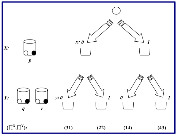
Figure 4.4: The conventional play of the two stage game features a closed room containing players $X$ and $Y$, their respective randomizing urns used to implement mixed strategies, and a large metallic apparatus featuring a ball, and different channels and cups to act as a decision recording device. Player $X$ implements their “$p$” randomization by draw either a white or black marble from their urn, and correspondingly drops the ball down the $x=0$ or $x=1$ channel. Player $Y$ picks up the ball, selects the relevant urn implementing either their “$q$” or “$r$” randomizations, draws either a white or black marble, and correspondingly drops the ball down the appropriate $y=0$ or $y=1$ channel into the waiting cups. Payoffs are assigned as shown.

4.3.1 Rational game play: A story

Let us make the mathematics more concrete by telling a story in an attempt to assist conceptualization of the new methods presented here.

Suppose that you are the first player, player $X$, in the example two stage game. As shown in Fig. 4.4, you are in a room with your opponent, player $Y$, and together, you are looking at the game playing equipment. As player $X$, you play first and have to drop a large ball down one of two channels marked $x=0$ or $x=1$. To assist your decision, you have an urn containing a prepared number of white or black marbles allowing you to implement a randomized mixed strategy by selecting $x=0$ with probability $1-p$ or $x=1$ with probability $p$. You have chosen $p$ so as to maximize your payoff. You are also aware that after your ball has landed in the appropriate cup, your opponent, player $Y$, will choose one of their two randomizing urns which each contain appropriate numbers of white and black marbles. The first urn allows player $Y$ to choose $y=0$ with probability $1-q$ and $y=1$ with probability $q$, while the second urn allows them to choose $y=0$ with probability $1-r$ and $y=1$ with probability $r$. Player $Y$ has chosen $q$ and $r$ so as to maximize their payoff. After determining their choice of $y=0$ or $y=1$, player $Y$ will drop the ball down the appropriate channel so that it lands in the waiting cup to provide a permanent record of each players decisions. The players then divide a payoff accordingly as shown in Fig. 4.4. As shown in previous sections, a conventional analysis results in the play combinations $(x,y)=(0,1)$ and respective payoffs of $\left(\langle\Pi^{X}\rangle,\langle\Pi^{Y}\rangle\right)=(2,2)$. The above situation captures the conventionally mandated procedure for payoff maximization in this particular strategic interaction. It is presumed that the specified use of the respective urns by each player along with the conventional analysis specifying the values of $p$, $q$ and $r$ suffices to optimize player payoffs. What could be simpler?

Notice however that game theory has never provided a proof that the above procedure is complete, necessary, or sufficient. In particular, von Neumann and Morgenstern explicitly used a method of “indirect proof” subject to later falsification and so did not prove the completeness, the necessity, or the sufficiency of their methods. Nash simply adopted a mixed strategy probability space as the simplest way to provide an existence proof for what are now called Nash equilibria. Kuhn established only that mixed and behavioral probability spaces were equivalent in games of perfect recall, but did not establish that they were complete, necessary, or sufficient. In fact, no-one has ever provided a mathematical proof of the completeness, the necessity, or the sufficiency of preferring one probability space over all others. Absent such proof, we suggest that rational players will explore every feasible probability space describing any given game. In the absence of any confirmed decision procedure mandating the use of one probability space over all others, we suppose that players have the capacity to examine alternate probability spaces, and choose between them so as to maximize their payoffs.

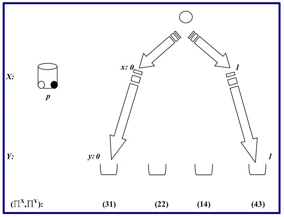
Figure 4.5: The correlated play of the two stage game features players $X$ and $Y$ and an altered decision recording apparatus. Player $X$ implements their “$p$” randomization as usual and drops the ball down either the $x=0$ or $x=1$ channel. Player $Y$ has used their toolkit to alter the device so they no longer have any decision to make as the ball simply continues falling down an extended channel to the waiting cups. Payoffs are assigned as shown.

Accordingly, suppose now that player $Y$ adopts a different procedure to that conventionally mandated. Suppose in fact that player $Y$ walks into the game room equipped with a toolkit containing hacksaws, hammers, and welding equipment, and suppose that before the game commences they set to work to reconfigure the decision recording device. As player $X$, you gaze in appalled fascination as $Y$ hammers, cuts, and welds away until the result is as shown in Fig. 4.5. As the time to start the game approaches, you have a decision to make. Your eyes provide you with evidence that the decision making device has been altered. Your previous analysis was based on the conventionally mandated device structure, but its alteration makes the previous analysis irrelevant and in all likelihood, wrong. As player $X$, you might seek to remonstrate with your opponent by saying that they cannot alter the definition of the game and that it is mandatory that they use the conventionally mandated space. In response, player $Y$ simply responds that they have not altered the game structure in any way, but have merely adopted a probability space which correlates their decision to the previous choice by $X$. Every single move of the game is still present but some have zero probability assigned. This is always possible. Conventional analysis allows such assignments of zero probability but then insists that these assignments can be altered by gradient optimization operations. In contrast, $Y$ asserts that they have assigned zero probabilities to certain moves which cannot be altered by gradient optimization operations as is specifically allowed by probability measure theory. Further, $Y$ knows of no proof proving the conventional mandate, and as they are solely motivated by a desire to maximize their payoff, they will take any steps appropriate to that goal. Your decision is whether to close your eyes to the altered nature of the decision making device and continue to argue that any such alteration is irrational and non-payoff maximizing, or to take the evidence of your eyes into account and to alter your analysis. What decision will you make? Self-evidently, as player $X$, after the game has commenced, you will now choose to drop your ball down the $x=1$ channel as that maximizes your payoff. Any other choice will minimize your payoff, and as a payoff maximizing rational player, you will not make such a choice. The result, as shown in previous sections, is that a correlated analysis results in the play combinations $(x,y)=(1,1)$ and respective payoffs of $\left(\langle\Pi^{X}\rangle,\langle\Pi^{Y}\rangle\right)=(4,3)$. This provides an increased payoff for player $Y$ justifying their rebuilding of the decision recording device.

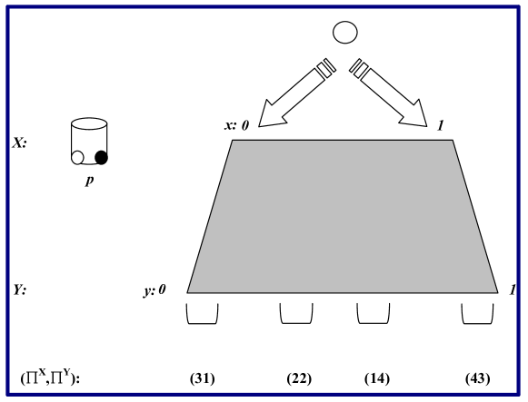
Figure 4.6: The play of the two stage game when player $X$ is unsure how player $Y$ has reconstructed the decision recording apparatus. Player $X$ implements their “$p$” randomization as usual and drops the ball down either the $x=0$ or $x=1$ channel. Player $Y$ might be using the conventional apparatus of Fig. 4.4 or the correlated apparatus of Fig. 4.5. Payoffs are assigned as shown.

But that doesn’t end the story as it is entirely unreasonable that player $X$ perfectly knows how $Y$ is making their decisions. We now suppose that you, as player $X$, have watched your opponent walk into the game room with their toolkit and a large rectangular metal shield. Player $Y$ erects their shield to entirely hide their part of the decision making device from your gaze, and behind this shield, they proceed to saw, hammer and weld away. You, as player $X$, are however entirely unsure what $Y$ is doing behind their shield. Perhaps $Y$ is reconstructing the original channel arrangements of the conventionally mandated device of Fig. 4.4. Perhaps on the other hand, player $Y$ is leaving the channels exactly as configured in the correlated decision device of Fig. 4.5 and the welding is required to reconstruct the required “$q$” and “$r$” urns. The resulting situation, as perceived by yourself, is as shown in Fig. 4.6. Here, both you and player $Y$ are depicted as being certain about how player $X$ will optimize their payoff. Namely, $X$ will use an urn to implement some mixed strategy “$p$” to optimize their payoff. However, you, as player $X$ have no information about how player $Y$ will make their decision. Again, you have a decision to make. A conventional analysis mandates that player $Y$ should use a conventionally configured decision device and you should play accordingly. In this case, $Y$ will gain a payoff of $\langle\Pi^{Y}\rangle=2$. However, $Y$ could alternatively choose to adopt a correlated probability space in which case they will gain a payoff of $\langle\Pi^{Y}\rangle=3$. Being rational, $Y$ can be expected to seek to maximize their expected payoff. What will you do? Will you assume that $Y$ has adopted a conventionally mandated space and drop the ball down the $x=0$ channel in the hope that it stops half way requiring $Y$ to walk over to the device to place it in the $y=1$ channel. What a disappointment then if the ball drops all the way down both the $x=0$ and $y=0$ channels into the leftmost cup. Or alternatively, will you assume that $Y$ is indeed a payoff maximizer able to alter their choice of decision device leading to the conclusion that $Y$ will have chosen to reconfigure the channels to implement correlated play. In this case, you should drop the ball into the $x=1$ channel in the hope that the ball will drop all the way through both the $x=1$ and $y=1$ channels into the rightmost cup. What a disappointment then if you see the ball stop half way requiring $Y$ to walk over to place the ball into the $y=0$ channel. What is your choice?

We suggest that if you know (by observing) that $Y$ has perfectly correlated their choice of $y$ to your choice of $x$, then you must take this information into account. Similarly, even without direct observation, if you can deduce that $Y$ will perfectly correlate their choice of $y$ to your choice of $x$, then likewise, you must take this information into account.

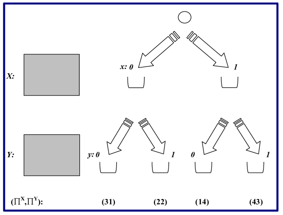
Figure 4.7: The play of the two stage game when both player $X$ and player $Y$ are unsure about which probability spaces and randomization devices have been adopted by their opponents. In this case, each player perfectly shields their decision making apparatus from their opponent (shaded devices), and so might be adopting the conventionally mandated analysis or any of an infinite number of alternate possible probability spaces. Rational players will analyze all these possibilities in order to maximize their payoffs. Payoffs are assigned as shown.

In reality of course, the situation in a real strategic exchange is more akin to that shown in Fig. 4.7. Here, each player knows precisely the rules of the game including all possible moves in their specified sequences. What they don’t know is the choice of probability space made by their opponent. This ignorance is represented by the coloured shields shown in the figure. In fact, prior to their completing their own analysis, they do not know which probability space they will adopt, or whether they will choose a single space or randomize over a number of spaces. This is in sharp contrast to the presumption of conventional game theory which mandates that each player must use a particular probability space (or one of their equivalents). As noted above, there has never been a proof of the completeness, necessity or sufficiency of this mandated type of space. In view of this, we suggest that rational players will simply optimize their choice of probability space to maximize their expected payoff. In Fig. 4.7, you, as player $X$, must deduce which space player $Y$ will use to maximize their payoff. In the situation depicted here, $Y$ has not physically reconstructed the decision recording device before your eyes, but they have likely chosen to adopt a particular probability space and physical randomization device. Their roulette might involve their preprogramming one or more random number generators, or might involve their providing instructions to an agent who will act autonomously once the game has begun allowing $Y$ to leave the room and take no further part in the game. As player $X$, you have absolutely no information whatsoever about which roulette will be adopted by $Y$. The only fact you are sure of is that $Y$ will act so as to maximize their payoff.

The question is, as always, is it possible for $Y$ to vary their choice of probability space, of their roulette, or is this impossible? If it is impossible, provide a proof of this conjecture, and then optimize accordingly. If it is possible, determine your optimal choices taking into account your opponent’s optimal choices.

4.4 Discussion

We propose that rational players will optimize their expected payoff functionals (not functions) in strategic situations using generalized calculus of variations approaches. These generalized variational functional optimization methods examine every possible value of a functional at every point as well as every possible gradient through that point. A rational player, seeking to perform a complete optimization, must examine every one of these possibilities against all of the equivalent range of possibilities of their opponents. These generalized methods give access to an infinity of non-independent and functionally constrained probability measure spaces defining non-continuous expected payoff functionals defined over discontinuous domains possessing, perhaps, a gradient nowhere.

The resulting generalized optimization approach corresponds to optimizing an infinite number of alternate game decision trees exhibiting altered optimal pathways and equilibria.

In this work, we follow the same methodology used by von Neumann and Morgenstern [1]. These authors initially focussed on single players, typified by Robinson Crusoe, who tried to optimize their payoff by choosing their actual moves or pure strategies in a consumption game. They then showed that this optimization method (focussed solely on pure strategies) did not generalize to all multiple player games leading to the introduction of probability distributions over pure strategies, defining mixed strategies. That is, it was established by these and later authors that while certain games (single player or multiple-player-perfect-information games) had solutions in pure strategies, this was not always true of more general games, and as a mixed strategy analysis entirely subsumes a pure strategy analysis, it was always advisable for a rational player to perform a complete mixed strategy analysis for general games. Here, we suggest similar results. It seems to be sufficient to employ conventional analysis for single-player or multiple-player-single-stage games. However, we suggest that the complete analysis of multiple-player-multiple-stage games requires more than a conventional analysis. Again, as the conventional analysis is entirely subsumed within our augmented optimization approach, it seems advisable for rational players to perform an augmented analysis in general.

In earlier chapters, we have alluded to the possibility that our expanded optimization analysis would produce results which differ from standard results in game theory. This does not mean that game theory is wrong. Just as a theorem valid in a flat geometry—the interior angles of all triangles sum to 180 degrees—can be invalid in a curved geometry, then so can results validly derived in game theory be invalid in our extended analysis. Game theory is incomplete, rather than wrong.

For instance, Kuhn established that games of perfect recall could always be decomposed into discreet subgames, and that the equilibrium pathway of the entire game consisted of concatenated portions of the equilibrium pathways of all the relevant subgames [4]. Crucial to the proof of this result, is the separability of the joint probability distributions of the entire game, and such separability exists only for the independent behavioural probability spaces developed by Kuhn. In our approach, behavioural strategies are not necessarily independent so their governing probability spaces are not necessarily separable. A theorem derived assuming that probability distributions is separable, is not applicable when distributions are inseparable.

Similarly, in the same paper, Kuhn established that games of perfect information always have pure strategy equilibria [4]. In our approach, even in perfect information games, players are uncertain about which probability space might be adopted by their opponents, and this allows equilibria to be probabilistic. Again, there is no contradiction with existing results, as theorems derived assuming separable probability distributions are inapplicable when distributions are inseparable.

All of the results and theorems of game theory are derived under certain assumptions about the joint probability spaces governing game analysis. When players can adopt alternate probability spaces invalidating these assumptions, then naturally, they can derive results which differ from those of game theory. Such differences reflect limitations in the optimization analysis of game theory, rather than errors in our more general optimization approach.

Finally, we again remind ourselves that conventional analysis routinely predicts outcomes at odds with observation. As we later show, the extended analysis that we argue must be available to players of unbounded rationality, will produce outcomes entirely consistent with observation.

Obviously, there are immediate applications of our new methods to sequential games such as the chain store paradox, the trust game, the ultimatum game, the public goods game, the centipede game, and the iterated prisoner’s dilemma. We turn to this now.

Chapter 5 Correlated Equilibria

5.1 Introduction

We are introducing isomorphism constraints into the strategy spaces of game theory. These constraints alter strategy space geometries to allow the location of new equilibria. It is useful to contrast out approach with Aumann’s “correlated equilibria”.

5.2 Correlated equilibria

In 1974, Aumann modeled a nominally competitive game in which players coopt public roulettes and share information to improve their payoffs. This possibility arises as the Nash equilibria for non-communicating players has them locating the best payoff regardless of their opponent’s choices so correlated changes of strategy are impossible. Given the ability to communicate however, correlated strategies become possible allowing novel equilibria. Following Aumann’s terminology, these are now termed “correlated equilibria”.

Our work here differs from Aumann’s approach. We allow players to alter their chosen private randomization devices but do not permit communication between players. We show that even without additional communication channels, if players use different physical randomization devices with different numbers of independent coordinates and functionally constrained coordinates, then these possible probability spaces must be taken into account. To clarify the difference and similarities between our entirely non-communicating analysis and Aumann’s correlated equilibria, we here go through one of the examples used by Aumman in detail.

To model correlated equilibria, Aumman introduced probability measures into his definitions of needed

equipment for randomizing strategies, and for defining utilities and subjective probability for the players. Thus to the description of the game we append the following:

(5) A set $\Omega$ (the states of the world), together with a $\sigma$-field ${\cal B}$ of subsets of $\Omega$ (the events);

(6) For each player $i$, a sub-$\sigma$-field ${\cal I}_{i}$ of ${\cal B}$ (the events in ${\cal I}_{i}$ are those regarding which $i$ is informed).

(7) For each player $i$, a relation $\succeq_{i}$ (the preference order of $i$) on the space of lotteries on the outcome space $X$, where a lottery on $X$ is a ${\cal B}$-measurable function from $\Omega$ to $X$ [23].

This welter of definitions was made understandable by use of a series of worked examples, and we here follow the same route by examining in detail Aumann’s example (2.7).

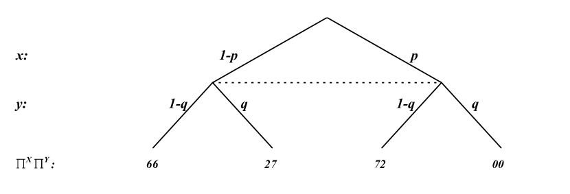
Figure 5.1: The game tree for the two player non-zero-sum game considered by Aumann in his example (2.7) [23]. Here, two players $X$ and $Y$ simultaneously and independently choose one of two options $x,y\in\{0,1\}$ to gain the payoff combinations shown.

In Aumman’s example (2.7), the two-person payoff matrix is

$$\begin{array}[]{cc}&P_{y}\\ P_{x}&\begin{array}[]{c|cc}(\Pi^{X},\Pi^{Y})&0&1\\ \hline\cr 0&(6,6)&(2,7)\\ 1&(7,2)&(0,0)\\ \end{array}\end{array}.$$ (5.1)

In terms of the behavioural probability space defined in Fig. 5.1, the expected payoff optimization problems are

$$X:\max_{p}\;\;\langle\Pi^{X}\rangle = 6+p-4q-3pq$$

$$Y:\max_{qr}\;\;\langle\Pi^{Y}\rangle = 6-4p+q-3pq.$$ (5.2)

These expected payoffs are continuous multivariate functions dependent only on the freely varying parameters $(p,q)$ so the relevant gradient operator used by both players to analyze this particular probability space is

$$\nabla=\left[\frac{\partial}{\partial p},\frac{\partial}{\partial q}\right].$$ (5.3)

Optimization then proceeds as usual via

$$\frac{\partial\langle\Pi^{X}\rangle}{\partial p} = 1-3q$$

$$\frac{\partial\langle\Pi^{Y}\rangle}{\partial q} = 1-3p$$ (5.4)

so equilibria appear at the intersections shown in Fig. 5.2. As noted by Aumann, there are three Nash equilibria for this game at choices $(p,q)=(0,1)$, $(1,0)$, and $(\frac{1}{3},\frac{1}{3})$ generating respective payoffs $(\langle\Pi^{X}\rangle,\langle\Pi^{Y}\rangle)=(2,7)$, $(7,2)$, and $(\frac{14}{3},\frac{14}{3})$.

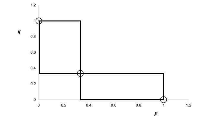
Figure 5.2: The intersection of the gradient conditions specifying Nash equilibria for the two player non-zero-sum game considered by Aumann in his example (2.7) [23]. The three Nash equilibria points are circled.

Aumann now supposes that the players share a public 3-sided fair dice allowing events “A”, “B”, and “C” to be selected with probability $\frac{1}{3}$, and that $X$ is informed whether or not event “A” appeared, while $Y$ is told whether or not “C” appeared. Aumann then asks, given this altered environment with additional communications, how will players now optimize their expected payoffs. As a first step, the players must alter their probability spaces to reflect the changed physical randomization devices being used.

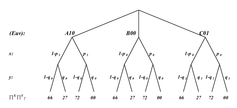
Figure 5.3: The modified game tree corresponding to the players sharing a three-sided dice selecting an event $E=A$, $B$, or $C$ with equal probability $\frac{1}{3}$ with player $X$ advised whether event $A$ occurs or not (specified by the indicator variable $u$) while player $Y$ is advised whether event $C$ occurs or not (indicated by the indicator variable $v$). The players can then appropriately condition their decisions on their available information sets, as indicated. The respective information sets are not adequately represented on this figure.

One possibility is depicted Fig. 5.3. Here, event $E\in\{A,B,C\}$ occurs each with probability of $1/3$ and conditions two additional variables $u,v\in\{0,1\}$. Player X knows the value of the variable $u$ while player $Y$ knows the value of $v$. The variable $u$ is set to $u=1$ when $E=A$ and $u=0$ otherwise, while $v=1$ when $E=C$ and $v=0$ otherwise. The players can condition their subsequent choices on the $u$ and $v$ variables.

The altered expected payoff functions are then

$$X:\max_{P^{X}}\;\;\langle\Pi^{X}\rangle = \sum_{Euv,x,y}P(Euv,x,y)\Pi^{X}(x,y)$$

$$= \sum_{Euv,x,y}P(Euv)P^{X}(x|Euv)P^{Y}(y|Euv)\Pi^{X}(x,y)$$

$$= \frac{1}{3}\left[18+2p_{0}+p_{1}-8q_{0}-4q_{1}-3\left[p_{1}q_{0}+p_{0}q_{0}+p_{0}q_{1}\right]\right]$$

$$Y:\max_{P^{Y}}\;\;\langle\Pi^{Y}\rangle = \sum_{Euv,x,y}P(Euv,x,y)\Pi^{Y}(x,y)$$ (5.5)

$$= \sum_{Euv,x,y}P(Euv)P^{X}(x|Euv)P^{Y}(y|Euv)\Pi^{Y}(x,y)$$

$$= \frac{1}{3}\left[18-8p_{0}-4p_{1}+2q_{0}+q_{1}-3\left[p_{1}q_{0}+p_{0}q_{0}+p_{0}q_{1}\right]\right].$$

written in terms of the joint probability distribution $P(Euv,x,y)$ spanning the probability space, and where we recognize that the payoff functions $\Pi^{Z}(x,y)$ depend only on the choices $x$ and $y$, and we also take account of the various conditioning possibilities of the variables.

Consequently, in this expanded probability space the relevant gradient operator is

$$\nabla=\left(\frac{\partial}{\partial p_{0}},\frac{\partial}{\partial p_{1}},\frac{\partial}{\partial q_{0}},\frac{\partial}{\partial q_{1}}\right)$$ (5.6)

in terms of which the players evaluate

$$\frac{\partial\langle\Pi^{X}\rangle}{\partial p_{0}} = \frac{1}{3}(2-3q_{0}-3q_{1})$$

$$\frac{\partial\langle\Pi^{X}\rangle}{\partial p_{1}} = \frac{1}{3}(1-3q_{0})$$

$$\frac{\partial\langle\Pi^{Y}\rangle}{\partial q_{0}} = \frac{1}{3}(2-3p_{0}-3p_{1})$$

$$\frac{\partial\langle\Pi^{Y}\rangle}{\partial q_{1}} = \frac{1}{3}(1-3p_{0}).$$ (5.7)

The second and fourth lines here specify that

$$p_{1} = \left\{\begin{array}[]{ll}1&\mbox{if }q_{0}<\frac{1}{3}\\ &\\ \mbox{arbitrary}&\mbox{if }q_{0}=\frac{1}{3}\\ &\\ 0&\mbox{if }q_{0}>\frac{1}{3}\\ \end{array}\right.$$ (5.13)

$$q_{1} = \left\{\begin{array}[]{ll}1&\mbox{if }p_{0}<\frac{1}{3}\\ &\\ \mbox{arbitrary}&\mbox{if }p_{0}=\frac{1}{3}\\ &\\ 0&\mbox{if }p_{0}>\frac{1}{3}\\ \end{array}\right.,$$ (5.19)

which in turn allows calculating the flow diagram for the remaining gradients in terms of the variables $p_{0}$ and $q_{0}$ as shown in Fig. 5.4. This locates two unstable stationary points at $(p_{0},q_{0})=(\frac{1}{3},\frac{1}{3})$ and $(\frac{2}{3},\frac{2}{3})$ and three stable stationary points defining correlated equilibria at $(p_{0},q_{0})=(0,0)$, $(0,1)$, and $(1,0)$. The respective payoffs for each player at these correlated equilibria points are $(\langle\Pi^{X}\rangle,\langle\Pi^{Y}\rangle)=(5,5)$, $(2,7)$, and $(7,2)$. There is then an additional correlated equilibria giving an increased expected payoff for each player motivating them to use the additional available information to correlate their strategy choices to their opponent’s moves.

Figure 5.4: The flow diagram showing the direction of the gradient of the respective expected payoffs $[\frac{\partial\langle\Pi^{X}\rangle}{\partial p_{0}},\frac{\partial\langle\Pi^{Y}\rangle}{\partial q_{0}}]$ identifying two unstable stationary points at $(p_{0},q_{0})=(\frac{1}{3},\frac{1}{3})$ and $(\frac{2}{3},\frac{2}{3})$ (open circles), as well as three stable stationary points locating correlated equilibria at $(p_{0},q_{0})=(0,0)$, $(0,1)$, and $(1,0)$ (closed disks). The respective payoffs at the correlated equilibria are $(\langle\Pi^{X}\rangle,\langle\Pi^{Y}\rangle)=(5,5)$, $(2,7)$, and $(7,2)$.

The location of a correlated equilibrium point with improved payoffs to both players, $(\langle\Pi^{X}\rangle,\langle\Pi^{Y}\rangle)=(5,5)$, lying strictly outside the convex hull of the Nash equilibrium payoffs concludes Aumann’s example. To reiterate, every change of the physical randomization device adopted by players, whether secret or public, must be modelled by altered probability spaces. Aumann introduced these tools to model correlated equilibria generated by players sharing a public randomization device and shared communication. This communication means that novel correlated equilibria can be located even in two-player single stage games.

In contrast, our work with isomorphic constraints based on correlations eschews any additional communication between the players. Rather, players can adopt different secret randomization devices modelled by altered probability spaces possessing different dimensionality, continuity properties, differentiability conditions, and gradients, all of which allow the location of novel equilibria. The continued absence of communication between the players means that, as far as we can tell, novel constrained equilibria appear only in multiple-player-multiple-stage games.

Chapter 6 The chain store paradox

6.1 Introduction

The chain store paradox examines predatory pricing to maintain monopoly profits. It gains its “paradoxical” moniker as (so it has been argued [24]) a substantial proportion of the economics profession finds itself disagreeing with the clear predictions of game theory in this game. That is, many economists would hold that it is irrational for any firm to engage in predatory pricing to drive rivals out of business and so gain a monopolist position as predation is costly to the predator while potential new entrants well understand that any price cutting is temporary. It is also generally held that any attempt to extract monopoly pricing benefits in some industry would quickly attract new entrants so any monopoly gains will be short lived. An extensive literature has demonstrated the implausibility of these claims, with Ref. [24] examining predatory pricing in the shipping industry, IBM pricing strategies against competitors, and coffee price wars, for instance.

Selton first proposed the chain store paradox as a complement to the finite iterated prisoner’s dilemma [25] in order to highlight inadequacies in game theory. These lacks would then justify the necessity of bounding rationality in game theory. Terming the conventional game theoretic analysis and predicted outcome as the “induction” argument, and contrasting this with an alternate “deterrence” theory, Selton noted

“…only the induction theory is game theoretically correct. Logically, the induction argument cannot be restricted to the last periods of the game. There is no way to avoid the conclusion that it applies to all periods of the game.

Nevertheless the deterrence theory is much more convincing. If I had to play the game in the role of [the monopolist], I would follow the deterrence theory. I would be very surprised if it failed to work. From my discussions with friends and colleagues, I get the impression that most people share this inclination. In fact, up to now I met nobody who said that he would behave according to the induction theory. My experience suggests that mathematically trained persons recognize the logical validity of the induction argument, but they refuse to accept it as a guide to practical behavior.

It seems safe to conjecture that even in a situation where all players know that all players understand the induction argument very well, [the monopolist] will adopt a deterrence policy and the other players will expect him to do so.

The fact that the logical inescapability of the induction theory fails to destroy the plausibility of the deterrence theory is a serious phenomenon which merits the name of a paradox. We call it the ‘chain store paradox’” [25].

Efforts to resolve the paradox include recognizing that players might not be sure that their opponents are rational payoff maximizers due to the impact of mistakes or trembles, rationality bounds, incomplete information, or altered definitions of rationality, all of which necessitate use of subjective probabilities [26]. In addition, introducing asymmetric information whereby entrants are uncertain whether monopolists are governed by behavioural rules which eliminate common knowledge of rationality and provide a rationale for entrants to base their expectations of the monopolist’s future behaviour on its past actions [24], while the use of imperfect information or uncertainty about monopolist payoffs allows the replication of observed behaviours [27]. Other approaches include dropping common knowledge of rationality [28], or by introducing incomplete and imperfect information [29]. For a good review of how this paradoxical game contributes to economic understanding appears, see [30].

Selton’s construction of the paradox hinges on the use of “deterrence” theory in a multiple stage game (involving repeated choices by the monopolist), whereby the monopolist can adopt a non-rational strategy in early stages of the game to build a reputation for implementing that strategy which induces their opponent’s to alter their own choices in latter stages. All subsequent treatments have followed Selton in modelling such multiple stage games and have then introduced some mechanism to justify “reputational” effects.

In contrast, in our treatment here, by introducing isomorphic constraints into our strategy spaces, we can establish that it is rational for the monopolist to adopt the seemingly irrational choice even in a minimal game (where the monopolist makes a single response to a single entrance) where it is commonly thought that reputation or deterrence effects cannot make an appearance. The conventional analysis of this minimal game is immediately solved via backwards induction dependent on the assumptions of a common knowledge of rationality (CKR), independent behavioural strategies defining separable joint probability distributions and allowing subgame decompositions. In our extended analysis, the adoption of isomorphically constrained joint probability spaces allows non-independent behavioural strategies described by non-separable joint probability distributions all of which invalidate subgame decompositions and alter the optima located via backwards induction. We demonstrate this now.

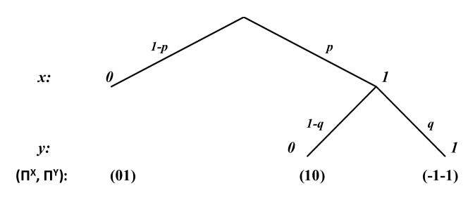
Figure 6.1: A minimal chain store game decision tree in an unconstrained behavioural space where a potential new market entrant $X$ must decide to either stay out of a new market $x=0$ with probability $1-p$ or enter the market $x=1$ with probability $p$, in which case the monopolist $Y$ chooses to either acquiesce $y=0$ with probability $1-q$ or fight $y=1$ with probability $q$ their entry, with the corresponding payoffs shown.

6.2 The chain store paradox

The minimal chain store paradox, conventionally pictured in Fig. 6.1, is defined over two sequential stages where first, a potential market entrant $X$ must decide to either stay out of a new market $x=0$ or enter that market $x=1$ where their opponent, the monopolist $Y$, observes this choice. Should $X$ stay out of the market, they neither gain nor lose any payoff while $Y$ gains monopolist profits so $(\Pi^{X},\Pi^{Y})=(0,1)$. In contrast, should $X$ enter the market, $Y$ must then decide whether to acquiesce to their opponent’s entry $y=0$ by leaving prices unchanged and losing profits so $(\Pi^{X},\Pi^{Y})=(1,0)$ or by driving $X$ out of business by price cutting so payoffs are $(\Pi^{X},\Pi^{Y})=(-1,-1)$.

6.2.1 Unconstrained behaviour strategy spaces

A standard analysis frames the behaviour strategy spaces of each player as being

$${\cal P}^{X}_{B} = \left\{x\in\{0,1\},\{1-p,p\}\right\}$$

$${\cal P}^{Y}_{B} = \left\{y\in\{0,1\},\{1-q,q\}|x=1\right\}.$$ (6.1)

Here, player $Y$ chooses their value of $y$ only when advised that $x=1$. In the joint behaviour space ${\cal P}^{X}_{B}\times{\cal P}^{Y}_{B}$, the respective optimization problems for the players are

$$X:\max_{p}\;\;\langle\Pi^{X}\rangle = p-2pq$$

$$Y:\max_{q}\;\;\langle\Pi^{Y}\rangle = 1-p-pq,$$ (6.2)

so the only independent parameters are $p$ and $q$. In this joint space, the gradient operator used by each player in their analysis is

$$\nabla=\left[\frac{\partial}{\partial p},\frac{\partial}{\partial q}\right],$$ (6.3)

so optimal solutions are obtained via

$$\frac{\partial\langle\Pi^{X}\rangle}{\partial p} = 1-2q$$

$$\frac{\partial\langle\Pi^{Y}\rangle}{\partial r} = -p.$$ (6.4)

The solutions to these conditions are graphed in Fig. 6.2. Here, the gradient of the payoff for the monopolist $Y$ is essentially always negative so $Y$ sets $q=0$ and so always acquiesces to new market entrants. In turn, realizing this, $X$ determines that the gradient of their payoff is always positive and so always sets $p=1$ and decides to enter the market. There is also an equilibria at the point $p=0$ and $q=1$, termed imperfect as it requires $Y$ to adopt an irrational strategy (to fight) when $X$ stays out of the market even though this intention cannot be sustained if indeed it turns out that $X$ enters the market. The resulting expected payoffs given that players adopt the sole perfect Nash equilibria of $p=1$ and $q=0$ are $\left(\langle\Pi^{X}\rangle,\langle\Pi^{Y}\rangle\right)=(1,0)$.

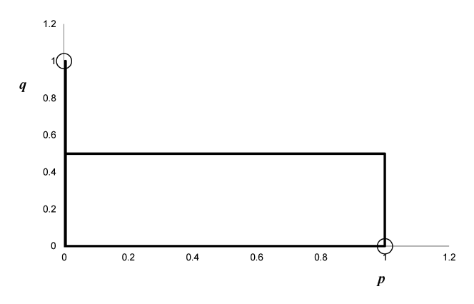
Figure 6.2: The intersection of the gradient conditions specifying Nash equilibria for the minimal chain store paradox. The two Nash equilibria points are circled.

It is useful to again remind ourselves how this conventional analysis without isomorphism constraints models perfect correlations between $x$ and $y$ to show that the monopolist cannot rationally sustain a perfectly correlated strategy. Suppose that $Y$ seeks to perfectly correlate $y$ with $x$ via $q=1$. As usual, both players are perfectly capable of evaluating the expected payoff gradients in the appropriate limit to obtain

$$\lim_{q\rightarrow 1}\frac{\partial\langle\Pi^{X}\rangle}{\partial p} = \lim_{q\rightarrow 1}(1-2q)\;=\;-1$$

$$\lim_{q\rightarrow 1}\frac{\partial\langle\Pi^{Y}\rangle}{\partial q} = \lim_{q\rightarrow 1}-p\;=\;-p.$$ (6.5)

That is, even when the monopolist seeks to perfectly correlate their choice $y$ with $x$, the non-zero gradients present at these points ensure they must rationally alter their intention so as to maximize their payoff. This conclusion is of course valid only when isomorphism constraints are absent so that behavioural strategy probability distributions are separable allowing subgame decompositions and optimization via backwards induction. Conversely, this result does not pertain when isomorphism contraints are in use.

Rational players of unbounded capacity are able to alter their choice of probability space, and will optimize this choice so as to maximize their expected payoffs. In each alternate space, the generated joint probability distributions might well involve non-independent variables so the joint probability distributions are nonseparable preventing conventional subgame decompositions and ensuring that novel equilibria can be located. We now complete a partial search of the possible joint probability spaces.

6.2.2 Isomorphically correlated space ${\cal P}^{X}_{B}\times{\cal P}^{Y}_{B}|_{q=1}$

Suppose that player $Y$ employs an isomorphism constraint $q=1$ ensuring that variable $y$ is perfectly correlated to $x$ via $y=x$ and $y^{2}=x^{2}=xy=x$. We denote this space ${\cal P}^{Y}_{B}|_{q=1}$. In this space, the optimization tasks facing the players are

$$X:\max_{x}\;\;\Pi^{X} = -x$$

$$Y:\;\;\Pi^{Y} = 1-2x.$$ (6.6)

It is immediately evident that player $X$ maximizes their payoff in this space by setting $x=0$. The same result arises when expected payoffs are used where we have the relations $\langle y\rangle=\langle x\rangle$ and $\langle y^{2}\rangle=\langle x^{2}\rangle=\langle xy\rangle=\langle x\rangle$ giving

$$X:\max_{p}\;\;\langle\Pi^{X}\rangle = -p$$

$$Y:\;\;\langle\Pi^{Y}\rangle = 1-2p.$$ (6.7)

As usual, the decision by $Y$ to adopt the ${\cal P}^{Y}_{B}|_{q=1}$ probability space leaves them with no further decisions to optimize. The relevant gradient operator used by both players to analyze this particular probability space is

$$\nabla = \frac{\partial}{\partial p}$$ (6.8)

so optimization proceeds as usual via

$$\frac{\partial\langle\Pi^{X}\rangle}{\partial p}=-1$$ (6.9)

ensuring that player $X$ chooses not to enter the market via $p=0$ giving $x=0$. Consequently, this means that $Y$ chooses $y=0$ but this setting does not influence payoffs. That is, when players $(X,Y)$ adopt the ${\cal P}^{X}_{B}\times{\cal P}^{Y}_{B}|_{q=1}$ joint probability space, they maximize their payoffs via the combination $(x,y)=(0,0)$ to garner payoffs $\left(\langle\Pi^{X}\rangle,\langle\Pi^{Y}\rangle\right)=(0,1)$. In short, the monopolist has deterred any new entry into the market so they retain their profit. The threat they made to retaliate was not empty and indeed, was sufficient to modify rational outcomes.

6.2.3 The functionally anti-correlated space: ${\cal P}^{X}_{B}\times{\cal P}^{Y}_{B}|_{q=0}$

Alternatively, player $Y$ might choose the alternate probability space ${\cal P}^{Y}_{B}|_{q=0}$ in which player $Y$ chooses to functionally anti-correlate their $y$ variable to the previous choice of $x$ via $y=1-x$ and $xy=0$. In the joint probability space ${\cal P}^{X}_{B}\times{\cal P}^{Y}_{B}|_{q=0}$, the expected payoff optimization problem becomes

$$X:\max_{x}\;\;\Pi^{X} = x$$

$$Y:\;\;\Pi^{Y} = 1-x.$$ (6.10)

It is immediately evident that player $X$ maximizes their payoff in this space by setting $x=1$. The use of expected payoffs will lead to the same result as we have the relations $\langle y\rangle=1-\langle x\rangle$ and $\langle xy\rangle=0$ giving

$$X:\max_{p}\;\;\langle\Pi^{X}\rangle = p$$

$$Y:\;\;\langle\Pi^{Y}\rangle = 1-p.$$ (6.11)

Again, the adoption of the ${\cal P}^{Y}_{B}|_{q=0}$ probability space leaves $Y$ with no decisions to optimize. As a result, the gradient operator is again

$$\nabla = \frac{\partial}{\partial p},$$ (6.12)

with optimization giving

$$\frac{\partial\langle\Pi^{X}_{0-}\rangle}{\partial p}=1,$$ (6.13)

ensuring that player $X$ chooses to enter the market via $p=1$ with $x=1$. Consequently, this means that $Y$ chooses $y=0$ but this setting does not influence payoffs. The result is that when players $(X,Y)$ adopt the ${\cal P}^{X}_{B}\times{\cal P}^{Y}_{B}|_{q=0}$ joint probability space, they maximize their payoffs via the combination $(x,y)=\{(1,0)\}$ to garner payoffs $\left(\langle\Pi^{X}\rangle,\langle\Pi^{Y}\rangle\right)=(1,0)$. In this space, $X$ is undeterred and enters the market to garner the profits

6.2.4 Expected payoff comparison across multiple probability spaces

Altogether, the various joint probability spaces which might be adopted by the players lead to a table of expected payoff outcomes of

$$\begin{array}[]{c|c}(\langle\Pi^{X}\rangle,\langle\Pi^{Y}\rangle)&{\cal P}^{X}_{B}\\ \hline\cr&\\ {\cal P}^{Y}_{B}|_{q=0}&(1,0)\\ &\\ {\cal P}^{Y}_{B}&(1,0)\\ &\\ {\cal P}^{Y}_{B}|_{q=1}&(0,1)\\ \end{array}$$ (6.14)

making it evident that to maximize their payoff, player $Y$ must rationally elect to use probability space ${\cal P}^{Y}_{B}|_{q=1}$ in preference to either ${\cal P}^{Y}_{B}$ or ${\cal P}^{Y}_{B}|_{q=0}$. That is, $Y$ will undertake to functionally correlate their choice to the previous choice of the potential market entrant, and thereby deny themselves a choice about the setting of $y$ once the game has commenced. They do this knowing it to be the payoff maximizing choice of probability space (among the few examined here). Knowing this, player $X$ will not enter the market even in this minimal chain store game. Similar results apply for extended games with multiple markets and potential entrants. The clear prediction of our analysis is that players of unbounded rationality will always fight entrants in the chain store game even though this strategy appears to be non-rational when examined using conventional analysis. That is, in the chain store game, a monopolist does not need to build a reputation for aggression over initial stages to try to discourage potential entrants in later stages. A monopolist, of unbounded rationality, is well aware that making a choice to adopt a probability space in which their choices are functionally assigned to be correlated to their opponent’s is both payoff maximizing and rational.

It is of course possible to consider a broader range of joint probability spaces for both players $X$ and $Y$, but these do not alter the conclusion here that it can be rational for a monopolist to punish market entrants to resolve the chain store paradox.

Chapter 7 The trust game

7.1 Introduction

The previous chapter considered what conventional analysis holds to be anomalous aggression, anomalous as it decreases the payoffs of the aggressive player. In this chapter, we consider trusting behaviour where players transfer their own payoffs to their opponent in the hope that their opponent will return the favour and transfer an enlarged pool of funds back to them. Needless to say, the conventional analysis holds that each of these trusting actions is anomalous. In this chapter, we consider the single shot trust game.

In earlier formulations, the trust game took place over repeated stages [31] allowing reputation and punishment theories to explain why players can exhibit trust and increase their payoffs over those predicted by game theory. Such results motivated investigations of single shot trust games (initially termed the investment game) where the minimal number of stages ensures that reputation and punishment effects are absent. Despite this, players continue to exhibit trust to increase their payoff [32]. More recently, players involved in the trust game have undergone functional magnetic resonance imaging of their brains during play [33]. Other minimal games eliminating reputation and punishment effects are the ultimatum and the dictator game among others.

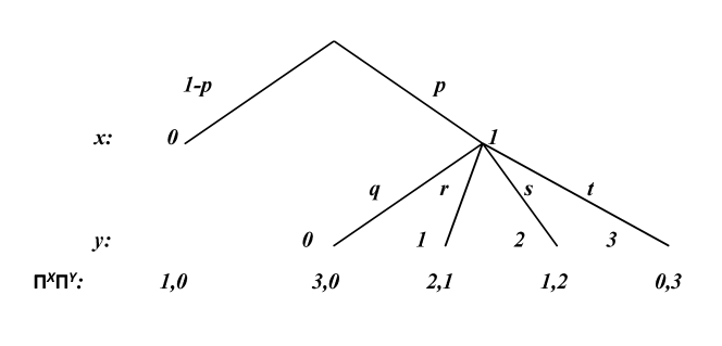
Figure 7.1: A minimal trust game wherein player $X$ possesses funds of one unit and must choose to either retain these funds $x=0$ generating payoffs of $\left(\Pi^{X},\Pi^{Y}\right)=(1,0)$ or trust their opponent by investing their funds with $Y$ via $x=1$. Should this investment occur, both players are aware that $Y$ receives three units, and must then decide how much of this total to keep and how much to return to $X$. That is, $Y$ decides to retain an amount $y\in\{0,1,2,3\}$ while returning an amount $3-y$ to $X$ generating payoffs of $\left(\Pi^{X},\Pi^{Y}\right)=(3-y,y)$.

7.2 A simplified trust game

In this section, we simplify the trust game as far as possible without losing any of its character.

The minimal trust game, as conventionally pictured in Fig. 7.1, is defined over two sequential stages where first, player $X$ possess a single unit of funds and must choose to either retain these funds $x=0$ generating payoffs of $\left(\Pi^{X},\Pi^{Y}\right)=(1,0)$, or trust their opponent by investing their funds with $Y$ via $x=1$. Should this investment occur, both players are aware that $Y$ receives three units and must then decide how much of this total to keep and how much to return to $X$. That is, $Y$ decides to retain an amount $y\in\{0,1,2,3\}$ while returning an amount $3-y$ to $X$ generating payoffs of $\left(\Pi^{X},\Pi^{Y}\right)=(3-y,y)$. Altogether, the payoffs to the players are

$$\Pi^{X} = 1-x+x(3-y)$$

$$\Pi^{Y} = xy.$$ (7.1)

7.2.1 Unconstrained behaviour strategy spaces

Conventional game analysis commences with the assumption that players $X$ and $Y$ each adopt a probability space lacking isomorphism constraints. Possible spaces include

$${\cal P}^{X}_{B} = \left\{x\in\{0,1\},\{1-p,p\}\right\}$$

$${\cal P}^{Y}_{B} = \left\{y\in\{0,1,2,3\},\{q,r,s,t\}|x=1\right\}.$$ (7.2)

Here, player $Y$ chooses their value of $y$ only when advised that $x=1$ and we have the normalization condition $q+r+s+t=1$. In the joint behaviour space ${\cal P}^{X}_{B}\times{\cal P}^{Y}_{B}$, the respective optimization problems for the players are

$$X:\max_{p}\;\;\langle\Pi^{X}\rangle = 1-p+p(3q+2r+s)$$

$$Y:\max_{q,r,s}\;\;\langle\Pi^{Y}\rangle = p(3-3q-2r-s).$$ (7.3)

The only independent variables here are $p,q,r$ and $s$ (subject to normalization constraints) so the relevant gradient operator is

$$\nabla=\left[\frac{\partial}{\partial p},\frac{\partial}{\partial q},\frac{\partial}{\partial r},\frac{\partial}{\partial s},\right].$$ (7.4)

Consequently, optimal solutions are obtained via

$$\frac{\partial\langle\Pi^{X}\rangle}{\partial p} = -1+3q+2r+s$$

$$\frac{\partial\langle\Pi^{Y}\rangle}{\partial q} = -3p$$

$$\frac{\partial\langle\Pi^{Y}\rangle}{\partial r} = -2p$$

$$\frac{\partial\langle\Pi^{Y}\rangle}{\partial s} = -p.$$ (7.5)

The last three equations here straightforwardly show that $Y$ maximizes their expected payoff by setting $q=r=s=0$ ensuring $t=1$ to give $y=3$. In turn, this result simplifies the optimization condition for $X$ establishing that $X$ maximizes their payoff by setting $p=0$ to give $x=0$. The Nash equilibria for this simplified trust game is then $(x,y)=(0,3)$ so both $X$ and $Y$ selfishly retain all the funds they can generating expected payoffs of $\left(\langle\Pi^{X}\rangle,\langle\Pi^{Y}\rangle\right)=(1,0)$.

As noted previously, these payoffs are not optimal as they could be improved by both players adopting different choices, as is commonly observed in human play.

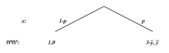
Figure 7.2: The case where players $(X,Y)$ adopt the ${\cal P}^{X}_{B}\times{\cal P}^{Y}_{B}|_{y=\bar{y}}$ joint probability space where player $Y$ functionally correlates their second stage choice to their opponent’s first stage choice. In this case, a decision by $X$ to invest funds with $Y$ automatically invokes a partial return of funds.

7.2.2 The isomorphically correlated space ${\cal P}^{X}_{B}\times{\cal P}^{Y}_{B}|_{y=\bar{y}}$

Rational players are able to alter their choice of probability space, and will optimize this choice so as to maximize their expected payoffs. Suppose that player $Y$ considers an alternate probability space denoted ${\cal P}^{Y}_{B}|_{y=\bar{y}}$ in which the choice of the variable $y$ is determined by the preceding choice of $x$ via

$$y=3(1-x)+x\bar{y}.$$ (7.6)

This means that when $x=0$ we have $y=3$ while the choice $x=1$ enforces the setting $y=\bar{y}$ for $\bar{y}\in\{0,1,2,3\}$. This possibility is shown in Fig. 7.2. Noting we still have $x^{2}=x$ and $x(1-x)=0$, the payoffs to each player are

$$X:\max_{x}\;\;\Pi^{X} = 1+x(2-\bar{y})$$

$$Y:\;\;\Pi^{Y} = x\bar{y}.$$ (7.7)

It is evident that player $X$ will set $x=1$ provided $\bar{y}<2$ and $x=0$ when $\bar{y}>2$. They are indifferent when $\bar{y}=2$ and so will play safe with $x=0$. The same results appear when the expected payoffs are maximized via

$$X:\max_{p}\;\;\langle\Pi^{X}\rangle = 1+2p-p\bar{y}$$

$$Y:\langle\Pi^{Y}\rangle = p\bar{y}.$$ (7.8)

The relevant gradient operator is

$$\nabla=\left[\frac{\partial}{\partial p}\right],$$ (7.9)

and optimization proceeds via

$$\frac{\partial\langle\Pi^{X}\rangle}{\partial p}=(2-\bar{y}).$$ (7.10)

As a result, $X$ maximizes their payoff by setting $p=1$ whenever $\bar{y}<2$, and $p=0$ otherwise. Subsequently, because $Y$ has left themselves no free choices during the game, the outcomes $(\bar{y},x,y,\langle\Pi^{X}\rangle,\langle\Pi^{Y}\rangle)$ are respectively $(0,1,0,3,0)$, $(1,1,1,2,1)$, $(2,0,3,1,0)$, and $(3,0,3,1,0)$.

7.2.3 Expected payoff comparison across multiple probability spaces

The optimal payoffs in the various joint probability spaces considered here which might be adopted by the players are

$$\begin{array}[]{c|c}(\langle\Pi^{X}\rangle,\langle\Pi^{Y}\rangle)&{\cal P}^{X}_{B}\\ \hline\cr&\\ {\cal P}^{Y}_{B}&(1,0)\\ &\\ {\cal P}^{Y}_{B}|_{y=0}&(3,0)\\ &\\ {\cal P}^{Y}_{B}|_{y=1}&(2,1)\\ &\\ {\cal P}^{Y}_{B}|_{y=2}&(1,0)\\ &\\ {\cal P}^{Y}_{B}|_{y=3}&(1,0)\\ \end{array}.$$ (7.11)

This makes it evident that to maximize their payoff, $Y$ must rationally elect to use the joint probability space ${\cal P}^{Y}_{B}|_{y=1}$ in preference to any alternate probability space considered here. That is, player $Y$ will undertake to functionally correlate their second stage decision to the previous choice of their opponent, and thereby deny themselves a second stage choice during the game knowing this to be the payoff maximizing choice. Knowing this, $X$ is confident enough to send all of their funds to $Y$ with the clear expectation of making a profit. This prediction of our extended analysis is in accord with observation.

Chapter 8 The ultimatum game

8.1 Introduction

The prevalence and importance of bargaining in society justifies the examination of simple bargaining models such as the ultimatum game, particularly in view of the discrepancy between observed player strategies and rational equilibrium solutions [34]. In the ultimatum game, two players must divide an item of equal utility to both (generally money). One player, the proposer, offers a proportional division to the other, the responder, who must either accept it in which case the division proceeds as suggested, or reject it in which case neither player receives any money. The assumption that players are rational and payoff maximizing allows derivation of the subgame perfect equilibrium where in each stage the proposer offers the smallest positive amount of money possible which the responder accepts as receiving some amount of money, however small, is always better than receiving none. This solution is seldom observed in experiments making the ultimatum game an ideal vehicle for testing the assumptions of game theory.

This role as a game theory test-bed has long been explored [35, 36, 34, 37, 38, 39, 40], and tested by many experiments including examination of the influence of variable stake sizes [41, 42, 43] and of culture [44, 45]. See experimental surveys in [46, 47, 48]. Experimental results typically demonstrate offers closer to a fair split (50%), and frequent rejections of offers even substantially above 0% (approximately the predicted equilibrium offer). Further, more detailed analysis shows that players, while failing to locate the subgame perfect equilibrium, are performing a sophisticated matching of offers to acceptance probabilities so as to maximize payoffs [49], while the ability to track a changing game environment demonstrates that proposers can be induced to vary their offer ranges and that responders can expand their acceptance sets—in effect offers and acceptances are contingent on the possibly changing game environment [50].

Proposed modifications to game theory to generate the observed payoff maximizing behaviour have focused on introducing mechanisms to complement player self-interest. In the main, these proposed additions either exploit modified utility functions interdependent on both player’s payoffs by taking account of psychological factors (so player utility increases with player equity or player intentionality say), or by embedding the ultimatum game within a larger, perhaps societal game (taking account of player reputation and self image for instance). These differing approaches include fairness [38, 51, 39, 44, 52, 53, 54, 55, 56, 57], though with equity definitions generally self-serving and modified by player information and payoff asymmetries [58], rivalry [59], reciprocity [60, 61], envy [62], punishment and revenge [63], competition and cooperation [64], altruism and spitefulness [65], and reputation [66]. In these approaches, player strategies effectively become contingent on both player’s payoffs generating novel equilibria allowing more equitable play.

Player learning can be modelled via algorithms modifying current strategy selections (offers and acceptance probabilities) in the light of prior game events [42, 67] which again makes player strategies contingent on those of their opponents to generate novel equilibria. See also [68, 69, 70]. Essentially the same algorithm can be implemented at the population level using evolutionary games theory in which players observe and learn about previous acceptances and rejections of other players and modify their strategies accordingly [71], or simply learn which payoff splits maximize payoffs [72]. See also [73, 74]. Again, these approaches effectively make current strategy choice contingent on prior game events to generate novel equilibria.

Figure 8.1: A conventional tree of the two stage ultimatum game. In this decision tree, $X$ makes an integral offer $1\leq x\leq M$ with probability $p_{x}$ to $Y$ who either accepts the offer by choosing $y=1$ with probability $q_{x}$ or who rejects the offer by setting $y=0$ with probability $1-q_{x}$. If the offer is accepted, the player payoffs are $(\Pi^{X},\Pi^{Y})=(M-x,x)$ while if the offer is rejected, player payoffs are $(\Pi^{X},\Pi^{Y})=(0,0)$.

8.2 The Ultimatum game

As shown in Fig. 8.1, the ultimatum game is defined here over two sequential stages where first $X$ communicates an integral offer $1\leq x\leq M$ to $Y$. Player $Y$ must then decide whether to accept the offer by choosing $y=1$ in which case $Y$ keeps the offer amount $x$ and $X$ receives an amount $M-x$. Alternately, $Y$ rejects the offer by choosing $y=0$ in which case neither player receives any payoff. That is, the payoffs are

$$\Pi^{X} = (M-x)y$$

$$\Pi^{Y} = xy.$$ (8.1)

A quick optimization analysis (achieved by straightforwardly embedding the discrete payoffs in the corresponding continuous functions) has

$$\frac{\partial\Pi^{X}}{\partial x} = -y<0$$

$$\frac{\partial\Pi^{Y}}{\partial y} = x>0,$$ (8.2)

indicating that player $X$ can increase their payoff by setting $x$ as small as possible, so $x=1$, while player $Y$ increases their payoff by making $y$ as large as possible, so $y=1$. This gives the equilibrium point $(x,y)=(1,1)$ generating payoffs of $(\Pi^{x},\Pi^{Y})=(M-1,1)$. However, few human players adopt this equilibrium point.

A more detailed analysis has players seeking to alter their choices of probability spaces ${\cal P}^{X}$ and ${\cal P}^{Y}$ so as to maximize their respective payoffs. As previously, players must determine which joint probability space defining the joint probability distributions will optimize payoff outcomes.

8.2.1 The isomorphically unconstrained space: ${\cal P}^{X}_{B}\times{\cal P}^{Y}_{B}$

The conventional analysis of the ultimatum game commences with players $X$ and $Y$ each adopting a probability space lacking isomorphism constraints. Possible spaces include

$${\cal P}^{X}_{B} = \left\{x\in\{1,2,\dots,M\},\{p_{1},p_{2},\dots,p_{M}\}\right\}$$

$${\cal P}^{Y}_{B} = \left\{y\in\{0,1\},\{P^{Y}(y=0|x=i)=(1-q_{i}),P^{Y}(y=1|x=i)=q_{i},\forall i\}\right\}.$$ (8.3)

Here, we have the normalization condition $\sum_{i}p_{i}=1$.

In the joint behaviour space ${\cal P}^{X}_{B}\times{\cal P}^{Y}_{B}$, the respective optimization problems for the players are

$$X:\max_{p_{2},\dots,p_{M}}\;\;\langle\Pi^{X}\rangle = q_{1}(M-1)-\sum_{i=2}^{M}p_{i}\left[q_{1}(M-1)-q_{i}(M-i)\right]$$

$$Y:\max_{q_{1},\dots,q_{M}}\;\;\langle\Pi^{Y}\rangle = q_{1}+\sum_{i=2}^{M}p_{i}(q_{i}i-q_{1}).$$ (8.4)

We have here resolved the normalization condition via $p_{1}=1-\sum_{i=2}^{M}p_{i}$. Consequently, the expected payoffs are continuous multivariate functions dependent on the probability parameters $(p_{2},\dots,p_{M},q_{1},\dots,q_{M})$, so the relevant gradient operator used by both players to analyze this particular probability space is

$$\nabla=\left[\frac{\partial}{\partial p_{2}},\dots,\frac{\partial}{\partial p_{M}},\frac{\partial}{\partial q_{1}},\dots,\frac{\partial}{\partial q_{M}}\right].$$ (8.5)

Immediately then, the optimization conditions evaluated by each player are

$$\frac{\partial\langle\Pi^{X}\rangle}{\partial p_{i}} = -[(M-1)q_{1}-(M-i)q_{i}],\;\;\;\forall i\in[2,M]$$

$$\frac{\partial\langle\Pi^{Y}\rangle}{\partial q_{i}} = ip_{i}\;\;\;\forall i\in[1,M].$$ (8.6)

The conditions for rates of change of $Y$’s payoff with respect to $q_{1},\dots,q_{M}$ here are all non-negative ensuring that $Y$ sets $q_{1}=\dots=q_{M}=1$ and thus accepts any offer from $X$ greater than or equal to $x=1$. In turn, these determinations simplify the optimization conditions for $X$ wherein the rates of change for $X$’s payoff with respect to all of $p_{2},\dots,p_{M}$ are negative so $X$ sets $p_{2}=\dots=p_{M}=0$ and $p_{1}=1$. The resulting choices by each player are $(x,y)=(1,1)$ generating expected payoffs of $\left(\langle\Pi^{X}\rangle,\langle\Pi^{Y}\rangle\right)=(M-1,1)$. This is the unique Nash equilibrium point for this ultimatum game, given the adoption of the joint probability space ${\cal P}^{X}_{B}\times{\cal P}^{Y}_{B}$. Unfortunately, it is not an equilibrium adopted by many human players.

Rational players will be very aware that both they and their opponent can alter their choice of probability space, and will optimize this choice so as to maximize their expected payoffs. In these alternate spaces, the random probability variables used in player optimizations might well be non-independent so joint probability distributions are nonseparable preventing conventional subgame decompositions and ensuring that novel equilibria can be located. We illustrate this now accomplishing, as usual, only a partial search of the available infinity of probability spaces.

8.2.2 An isomorphically constrained space: ${\cal P}^{X}_{B}\times{\cal P}^{Y}_{B}|_{y=\bar{y}}$

Suppose that player $Y$ adopts one of a possible $M-1$ alternate probability spaces ${\cal P}^{Y}_{B}|_{y=\bar{y}}$ for integral $2\leq\bar{y}\leq M$ in which they correlate their $y$ variable with the previous value $x$. In particular, suppose that $Y$ undertakes to reject any offer $x$ less than $\bar{y}$ and to accept any offer $x$ equal to or greater than $\bar{y}$. That is $Y$ adopts the functional assignment

$$y=\left\{\begin{array}[]{ll}0&\mbox{if }x<\bar{y}\\ &\\ 1&\mbox{if }x\geq\bar{y}.\\ \end{array}\right.$$ (8.7)

In other words, we have $y=\delta_{x\geq\bar{y}}$ giving the payoff functions

$$X:\max_{x}\;\;\Pi^{X} = (M-x)\delta_{x\geq\bar{y}}$$

$$Y:\;\;\Pi^{Y} = x\delta_{x\geq\bar{y}}.$$ (8.8)

It is then evident that player $X$ will set $x=\bar{y}$ to maximize their payoff at $\Pi^{X}=(M-\bar{y})$ giving player $Y$ a payoff of $\Pi^{Y}=\bar{y}$. Similar results are obtained from optimizing the expected payoff functions obtained using the probability distribution

$$P^{Y}(y|x)=\left\{\begin{array}[]{l}P^{Y}(y=0|x)=1-\sum_{j=\bar{y}}^{M}\delta_{jx}\\ \\ P^{Y}(y=1|x)=\sum_{j=\bar{y}}^{M}\delta_{jx}.\\ \end{array}\right.$$ (8.9)

Players of unbounded rationality must then sequentially assume that players $X$ and $Y$ have adopted the joint probability space ${\cal P}^{X}_{B}\times{\cal P}^{Y}_{B}|_{y=\bar{y}}$ for $2\leq\bar{y}\leq M$, and within each space, locate the constrained equilibria optimizing outcomes, all of which can be subsequently compared in a later comparison table. We complete this process now.

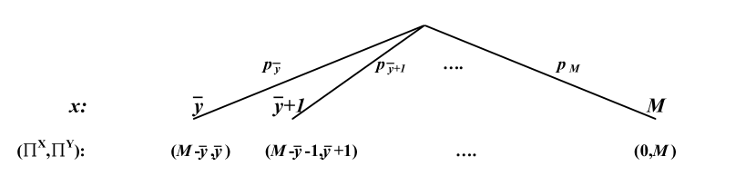
Figure 8.2: The case where players $(X,Y)$ adopt the ${\cal P}^{X}_{B}\times{\cal P}^{Y}_{B}|_{y=\bar{y}}$ joint probability space where player $Y$ is functionally constrained to reject any offer $x<\bar{y}$ and to accept any offer $x\geq\bar{y}$. As a result offers of a lesser amount appear neither in the expected payoff functions nor in the corresponding game tree.

With the adoption of the joint probability space ${\cal P}^{X}_{B}\times{\cal P}^{Y}_{B}|_{y=\bar{y}}$, and taking account of the the normalization condition $p_{\bar{y}}=1-\sum_{i=\bar{y}+1}^{M}p_{i}$, the expected payoff optimization problems for the players becomes

$$X:\max_{p_{\bar{y}+1},\dots,p_{M}}\;\;\langle\Pi^{X}\rangle = (M-\bar{y})+\sum_{i=\bar{y}+1}^{M}p_{i}(\bar{y}-i)$$

$$Y:\langle\Pi^{Y}\rangle = \sum_{i=\bar{y}}^{M}p_{i}i,$$ (8.10)

which are now dependent only on the freely varying parameters $(p_{\bar{y}+1},\dots,p_{M})$. That is, given their previous choice of probability space, player $Y$ has no further independent parameters, while player $X$ is indifferent to any choice with $1\leq i<\bar{y}$ because these variables have disappeared from the problem specification. The resulting game tree is as shown in Fig. 8.2. The relevant gradient operator used by both players to analyze this particular probability space is

$$\nabla = \left[\frac{\partial}{\partial p_{\bar{y}+1}},\dots,\frac{\partial}{\partial p_{M}}\right].$$ (8.11)

Optimization then proceeds as usual via

$$\frac{\partial\langle\Pi^{X}\rangle}{\partial p_{i}} = \bar{y}-i,\;\;\;\forall i\in[\bar{y}+1,M].$$ (8.12)

All of the terms on the right hand side are negative ensuring that player $X$ sets $p_{\bar{y}+1}=\dots=p_{M}=0$. In turn, this means that $X$ sets $p_{\bar{y}}=1$ and only ever offers $x=\bar{y}$. (When $\bar{y}=M$, player $X$ gains zero payoff regardless of their offer and so is indifferent.) Consequently, in the joint probability space ${\cal P}^{X}_{B}\times{\cal P}^{Y}_{B}|_{y=\bar{y}}$, players $(X,Y)$ choose the combination $(x,y)=\{(\bar{y},1)\}$ to garner payoffs $\left(\langle\Pi^{X}\rangle,\langle\Pi^{Y}\rangle\right)=(M-\bar{y},\bar{y})$.

8.2.3 Payoff comparison across probability spaces

The above analysis has considered a total of one conventional joint probability space ${\cal P}^{X}_{B}\times{\cal P}^{Y}_{B}$ and $M-1$ alternate probability spaces ${\cal P}^{X}_{B}\times{\cal P}^{Y}_{B}|_{y=\bar{y}}$ for $2\leq\bar{y}\leq M$. Altogether, the various joint probability spaces adopted by the players lead to a table of expected payoff outcomes of

$$\begin{array}[]{c|c}&\\ (\langle\Pi^{X}\rangle,\langle\Pi^{Y}\rangle)&{\cal P}^{X}_{B}\\ \hline\cr{\cal P}^{Y}_{B}&(M-1,1)\\ {\cal P}^{Y}_{B}|_{y=2}&(M-2,2)\\ \vdots&\vdots\\ {\cal P}^{Y}_{B}|_{y=M-2}&(2,M-2)\\ {\cal P}^{Y}_{B}|_{y=M-1}&(1,M-1)\\ \end{array},$$ (8.13)

making it evident that to maximize their payoff, player $Y$ must rationally elect to use probability space ${\cal P}^{Y}_{B}|_{y=M-1}$ in preference to ${\cal P}^{Y}_{B}$. Knowing this, player $X$ will offer $x=(M-1)$ to $Y$ to ensure that they gain a payoff greater than zero.

8.2.4 An indicative solution reflecting symmetries

Obviously, in normal play of the ultimatum game, $X$ does not normally expect that they need to offer all of the available funds to avoid rejection, and $Y$ seldom elects to reject every offer less than all of the funds. This might result as the game is now highly symmetric.

A conventional analysis shows that player $X$ can garner a payoff of $M-1$ and force $Y$ to accept a payoff of $1$. The isomorphic constrained analysis here shows that $Y$ can force a payoff of $M-1$ for themselves leaving $X$ with a minimal payoff of $1$. Player $X$, facing a minimal payoff of $1$ could then seek to modify their own probability space and undertake to not even consider offers greater than $\bar{x}$ say. It is possible that an extended analysis taking account of the ability of both $X$ and $Y$ to veto offers will settle in a choice around $\bar{x}=\bar{y}=M/2$ or thereabouts.

The analysis presented here is indicative only and we do not attempt to resolve the ultimatum game. It suffices for our purposes to show that including isomorphic constraints within the strategy spaces of the ultimatum game allows a broader range of equilibria outcomes than considered by conventional game theory.

8.3 Discussion

This paper presents an analysis of isomorphically constrained play in the finitely iterated Ultimatum game. The use of isomorphic constraints reduces the dimensionality of the game strategy spaces and can modify game properties and equilibrium points. We suggest that these constraints are routinely exploited in human play to maximize player outcomes. We crudely suggested that fair play might be one possible outcome of our extended analysis.

Experiments across a wide range of cultures show human players as commonly adopting fair play. This carries the implication that human game players in a diversity of cultures have a natural ability to exploit isomorphic constraints to their own ends. Further, we suggest that use of isomorphic constraints are common in bargaining situations and in economics in general, and it is necessary that games theory be able to properly model these isomorphic constraints in strategic interactions. Further, our analytical approach is likely to be more broadly applicable to the wider economic sphere as modeled by game theory.

Chapter 9 The public goods game

9.1 Introduction

There are many situations in which a number of players must jointly participate in creating some common resource but where no player can be prevented from exploiting that resource. This creates a “free-rider” or “tragedy of the commons” style problem as while all players benefit if the public good is provided, any individual player can increase their benefits if they avoid paying their share of the costs [75]. As a result, players do not cooperate and the public good is not provided. These results are altered if players are able to punish free riders, even when punishment carries significant costs to the initiator [76]. The public goods game allows experimental examination of how norms of cooperative behaviour are established and enforced using a wide range of theoretical approaches [77, 78, 79, 80], including a proposed quantum solution [81].

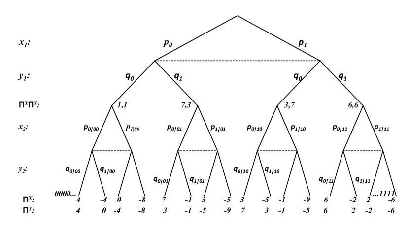
Figure 9.1: A minimal public goods game involving two players $X$ and $Y$ who simultaneously choose to make an investment of some amount $x_{1},y_{1}\in\{0,1\}$ in stage one. The return to each player of their own investment is negative whilst the return to them from their opponent’s investment is positive. Thus, investment is a public good which creates a free rider problem. In the second stage, each player can choose to either punish their opponent for their first stage actions $x_{2},y_{2}=1$ at some cost to themselves, or not $x_{2},y_{2}=0$, with the corresponding payoffs shown.

9.2 A simplified public goods game

Here as usual, we simplify the public goods game as far as possible without losing any of its character. In particular, we restrict the number of players to two, designated as usual $X$ and $Y$, and also restrict both the amounts that can be exchanged and the amounts used to punish opponents.

The minimal public goods game, as pictured in Fig. 9.1, is defined over two sequential stages. In stage one, players $X$ and $Y$ both choose whether four units of payoff is either retained $x_{1},y_{1}=0$ or invested $x_{1},y_{1}=1$. The return to each player from their own investment is negative whilst the return to them from their opponent’s investment is positive. The payoffs to the players from their joint actions in stage one are

$$\Pi^{X}_{1} = 4-x_{1}+3y_{1}$$

$$\Pi^{Y}_{1} = 4+3x_{1}-y_{1}.$$ (9.1)

Thus, should both $X$ and $Y$ make no investments via $x_{1}=y_{1}=0$ then their payoffs are $\Pi^{X}_{1}=\Pi^{Y}_{1}=4$ while if both invest all their funds via $x_{1}=y_{1}=1$ then their payoffs are improved to $\Pi^{X}_{1}=\Pi^{Y}_{1}=6$. Unfortunately however, it pays for each player to free ride on their opponent’s investment: should $X$ invest their funds $x_{1}=1$ while $Y$ retains all of their funds $y_{1}=0$, the joint payoffs are $\left(\Pi^{X}_{1},\Pi^{Y}_{1}\right)=\left(3,7\right)$, making it tempting for $Y$ to free ride. Conversely, should $X$ retain their funds while $Y$ invests, the payoffs are $\left(\Pi^{X}_{1},\Pi^{Y}_{1}\right)=\left(7,3\right)$. The net result is that game theory predicts that both players attempt to free ride on the investment of their opponent resulting in non-Pareto optimal payoffs.

The willingness of players to incur costs to punish their free riding opponents can then be studied by adding a second stage as shown in Fig. 9.1. Here, each player can choose to either not punish their opponent $x_{2},y_{2}=0$ leaving all payoffs unchanged, or can choose to punish their opponent $x_{2},y_{2}=1$ at some cost to themselves. That is, should a player choose to punish their opponent, they decrease their payoff by four units while at the same time decreasing their opponent’s payoff by eight units. Consequently, by the end of stage two, the joint payoffs are

$$\Pi^{X} = 4-x_{1}+3y_{1}-4x_{2}-8y_{2}$$

$$\Pi^{Y} = 4+3x_{1}-y_{1}-8x_{2}-4y_{2}.$$ (9.2)

It is this two stage form of the game that generates significant discrepancies between game theoretic predictions and observed human play. In particular, because punishment is costly then game theory makes the firm prediction that rational players will never choose to punish their opponents. However, precisely the opposite tends to occur in practise. People exhibit a strong tendency to punish their free riding opponents even when this reduces their own payoffs. Herein lies the interest in the public goods game.

9.2.1 Unconstrained behavioural strategy spaces: ${\cal P}^{X}_{B}\times{\cal P}^{Y}_{B}$

Conventional game analysis commences with the assumption that both players $X$ and $Y$ together adopt a joint probability space ${\cal P}^{X}_{B}\times{\cal P}^{Y}_{B}$ in which every behavioural strategy on every history set is independent. One possibility for the joint behavioural strategy space is shown in Fig. 9.1. We have chosen a terminology allowing the expected payoff function for player $Z\in\{X,Y\}$ to be written as

$$Z:\max\;\;\langle\Pi^{Z}\rangle = \sum_{x_{1},y_{1},x_{2},y_{2}=0}^{1}P^{XY}(x_{1},y_{1},x_{2},y_{2})\Pi^{Z}(x_{1},y_{1},x_{2},y_{2})$$ (9.3)

$$= \sum_{x_{1},y_{1},x_{2},y_{2}=0}^{1}P^{X}(x_{1})P^{Y}(y_{1})P^{X}(x_{2}|x_{1}y_{1})P^{Y}(y_{2}|x_{1}y_{1})\Pi^{Z}(x_{1},y_{1},x_{2},y_{2})$$

$$= \sum_{x_{1},y_{1},x_{2},y_{2}=0}^{1}p_{x_{1}}q_{y_{1}}p_{x_{2}|x_{1}y_{1}}q_{y_{2}|x_{1}y_{1}}\Pi^{Z}(x_{1},y_{1},x_{2},y_{2}).$$

We also have implicit normalization conditions such as $p_{0}+p_{1}=1$ and $p_{0|x_{1}y_{1}}+p_{1|x_{1}y_{1}}=1$, and so on. The expected payoff functions for each player are then

$$X:\max_{p_{1},p_{1|x_{1}y_{1}}}\;\;\langle\Pi^{X}\rangle = 4-\langle x_{1}\rangle+3\langle y_{1}\rangle-4\langle x_{2}\rangle-8\langle y_{2}\rangle$$

$$= 4-p_{1}+3q_{1}-4\sum_{x_{1}y_{1}x_{2}=0}^{1}p_{x_{1}}q_{y_{1}}p_{x_{2}|x_{1}y_{1}}x_{2}-8\sum_{x_{1}y_{1}y_{2}=0}^{1}p_{x_{1}}q_{y_{1}}q_{y_{2}|x_{1}y_{1}}y_{2}$$

$$= 4-p_{1}+3q_{1}-4\sum_{x_{1}y_{1}=0}^{1}p_{x_{1}}q_{y_{1}}p_{1|x_{1}y_{1}}-8\sum_{x_{1}y_{1}=0}^{1}p_{x_{1}}q_{y_{1}}q_{1|x_{1}y_{1}}$$

$$Y:\max_{q_{1},q_{1|x_{1}y_{1}}}\;\;\langle\Pi^{Y}\rangle = 4+3\langle x_{1}\rangle-\langle y_{1}\rangle-8\langle x_{2}\rangle-4\langle y_{2}\rangle$$ (9.4)

$$= 4+3p_{1}-q_{1}-8\sum_{x_{1}y_{1}x_{2}=0}^{1}p_{x_{1}}q_{y_{1}}p_{x_{2}|x_{1}y_{1}}x_{2}-4\sum_{x_{1}y_{1}y_{2}=0}^{1}p_{x_{1}}q_{y_{1}}q_{y_{2}|x_{1}y_{1}}y_{2}$$

$$= 4+3p_{1}-q_{1}-8\sum_{x_{1}y_{1}=0}^{1}p_{x_{1}}q_{y_{1}}p_{1|x_{1}y_{1}}-4\sum_{x_{1}y_{1}=0}^{1}p_{x_{1}}q_{y_{1}}q_{1|x_{1}y_{1}}.$$

Here, the expected payoff functions are continuous multivariate functions dependent on the probability parameters $\left[p_{1},p_{1|00},p_{1|01},p_{1|10},p_{1|11}\right]$ and $\left[q_{1},q_{1|00},q_{1|01},q_{1|10},q_{1|11}\right]$, so the relevant gradient operator is

$$\nabla = \left[\frac{\partial}{\partial p_{1}},\frac{\partial}{\partial p_{1|00}},\frac{\partial}{\partial p_{1|01}},\frac{\partial}{\partial p_{1|10}},\frac{\partial}{\partial p_{1|11}},\frac{\partial}{\partial q_{1}},\frac{\partial}{\partial q_{1|00}},\frac{\partial}{\partial q_{1|01}},\frac{\partial}{\partial q_{1|10}},\frac{\partial}{\partial q_{1|11}}\right].$$ (9.5)

Normalization conditions mean that any term dependent on $p_{0}$ or $p_{0|x_{1}y_{1}}$ contributes a negative term to any gradient with respect to $p_{1}$ or $p_{1|x_{1}y_{1}}$ respectively. Similar considerations apply to the $q$ parameters.

Taking account of normalization, the optimization conditions evaluated by each player are

$$\frac{\partial\langle\Pi^{X}\rangle}{\partial p_{1}} = -1+4\sum_{y_{1}=0}^{1}q_{y_{1}}\left(p_{1|0y_{1}}-p_{1|1y_{1}}\right)+8\sum_{y_{1}=0}^{1}q_{y_{1}}\left(q_{1|0y_{1}}-q_{1|1y_{1}}\right)$$

$$\frac{\partial\langle\Pi^{X}\rangle}{\partial p_{1|00}} = -4p_{0}q_{0}$$

$$\frac{\partial\langle\Pi^{X}\rangle}{\partial p_{1|01}} = -4p_{0}q_{1}$$

$$\frac{\partial\langle\Pi^{X}\rangle}{\partial p_{1|10}} = -4p_{1}q_{0}$$

$$\frac{\partial\langle\Pi^{X}\rangle}{\partial p_{1|11}} = -4p_{1}q_{1}$$

$$\frac{\partial\langle\Pi^{Y}\rangle}{\partial q_{1}} = -1+8\sum_{x_{1}=0}^{1}p_{x_{1}}\left(p_{1|x_{1}0}-p_{1|x_{1}1}\right)+4\sum_{x_{1}=0}^{1}p_{x_{1}}\left(q_{1|x_{1}0}-q_{1|x_{1}1}\right)$$

$$\frac{\partial\langle\Pi^{Y}\rangle}{\partial q_{1|00}} = -4p_{0}q_{0}$$

$$\frac{\partial\langle\Pi^{Y}\rangle}{\partial q_{1|01}} = -4p_{0}q_{1}$$

$$\frac{\partial\langle\Pi^{Y}\rangle}{\partial q_{1|10}} = -4p_{1}q_{0}$$

$$\frac{\partial\langle\Pi^{Y}\rangle}{\partial q_{1|11}} = -4p_{1}q_{1},$$ (9.6)

Thus, player $X$ finds the rate of change of their payoff with respect to $p_{1|ij}$ is always negative so they set $p_{1|ij}=0$ for all $i$ and $j$. Similarly, player $Y$ sets $q_{1|ij}=0$ as the rate of change of their payoff with respect to $q_{1|ij}$ is also always negative for all $i$ and $j$. That is, there are no histories in which it is payoff maximizing for either player to punish their opponent. In turn, these results simplify the remaining two conditions for first stage moves giving

$$\frac{\partial\langle\Pi^{X}\rangle}{\partial p_{1}} = -1$$

$$\frac{\partial\langle\Pi^{Y}\rangle}{\partial q_{1}} = -1.$$ (9.7)

This establishes that both players maximize their expected payoffs by setting $p_{1}=0$ and $q_{1}=0$ in the first stage. Thus, both players make no investment in the first round confident in the knowledge that their opponent will not punish them for this. The Nash equilibria for this simplified public goods game is then $(x_{1},y_{1},x_{2},y_{2})=(0,0,0,0)$ generating expected payoffs of $\left(\langle\Pi^{X}\rangle,\langle\Pi^{Y}\rangle\right)=(4,4)$. As noted previously, these payoffs are not Pareto optimal as they could be improved by both players adopting different choices, as is commonly observed in human play.

Rational players are able to alter their choice of probability space, and will optimize this choice so as to maximize their expected payoffs. We here suppose that players might each consider a total of two alternate probability spaces.

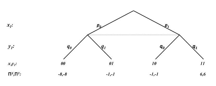
Figure 9.2: The case where players $(X,Y)$ adopt the ${\cal P}^{X}_{B}|_{x_{2}=1-y_{1}}\times{\cal P}^{Y}_{B}|_{y_{2}=1-x_{1}}$ joint probability space where both players functionally anti-correlate their second stage choices to their opponent’s first stage choices. Then a failure to invest automatically invokes punishment while investment invokes no punishment.

9.2.2 Isomorphically anti-correlated space ${\cal P}^{X}_{B}|_{x_{2}=1-y_{1}}\times{\cal P}^{Y}_{B}|_{y_{2}=1-x_{1}}$

Suppose first that both players $X$ and $Y$ choose to adopt a joint probability space ${\cal P}^{X}_{B}|_{x_{2}=1-y_{1}}\times{\cal P}^{Y}_{B}|_{y_{2}=1-x_{1}}$ as shown in Fig. 9.2, in which they each functionally anti-correlate their second stage choices to the previous choices of their opponents. This is implemented via

$$x_{2} = 1-y_{1}$$

$$p_{1|x_{1}y_{1}} = \delta_{1,(1-y_{1})}$$

$$y_{2} = 1-x_{1}$$

$$q_{1|x_{1}y_{1}} = \delta_{1,(1-x_{1})}.$$ (9.8)

This choice of probability space alters the dimensions of the game space, the game trees, and the payoff functions to be

$$\Pi^{X} = 4-x_{1}+3y_{1}-4x_{2}-8y_{2}$$

$$= 4-x_{1}+3y_{1}-4(1-y_{1})-8(1-x_{1})$$

$$= -8+7x_{1}+7y_{1}$$

$$\Pi^{Y} = 4+3x_{1}-y_{1}-8x_{2}-4y_{2}$$ (9.9)

$$= 4+3x_{1}-y_{1}-8(1-y_{1})-4(1-x_{1})$$

$$= -8+7x_{1}+7y_{1}.$$

It is then immediately evident that players maximize their own payoffs by choosing to invest $(x_{1},y_{1})=(1,1)$ which invokes a subsequent lack of punishment in stage two giving $(x_{2},y_{2})=(0,0)$. The final payoffs are then $(\Pi^{X},\Pi^{Y})=(6,6)$.

Optimization of the expected payoffs must reproduce this result. The isomorphically constrained expected payoff functions can simply be read from the tree in Fig. 9.2 and are

$$X:\max_{p_{1}}\;\;\langle\Pi^{X}\rangle = -8+7p_{1}+7q_{1}$$

$$Y:\max_{q_{1}}\;\;\langle\Pi^{Y}\rangle = -8+7p_{1}+7q_{1}.$$ (9.10)

These expected payoffs are continuous multivariate functions dependent only on the freely varying parameters $p_{1}$ and $q_{1}$, so the relevant gradient operator used by both players is

$$\nabla=\left[\frac{\partial}{\partial p_{1}},\frac{\partial}{\partial q_{1}}\right].$$ (9.11)

Immediately then, the optimization conditions evaluated by each player are

$$\frac{\partial\langle\Pi^{X}\rangle}{\partial p_{1}} = 7$$

$$\frac{\partial\langle\Pi^{Y}\rangle}{\partial q_{1}} = 7,$$ (9.12)

ensuring that both players $X$ and player $Y$ maximize their expected payoffs by investing their funds by setting $p_{1}=1$ giving $x_{1}=1$ and $q_{1}=1$ giving $y_{1}=1$. The functionally assigned punishment choices then ensure that neither player punishes the other so the equilibria choice of play is $(x_{1},y_{1},x_{2},y_{2})=(1,1,0,0)$ generating expected payoffs of $\left(\langle\Pi^{X}\rangle,\langle\Pi^{Y}\rangle\right)=\left(6,6\right)$.

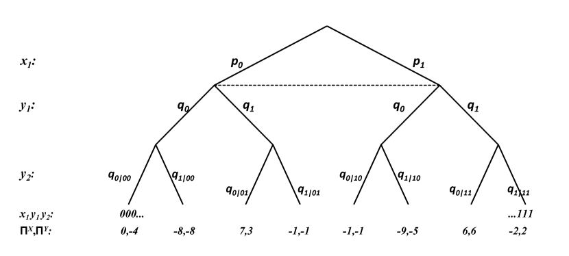
Figure 9.3: The case where players $(X,Y)$ adopt the ${\cal P}^{X}_{B}|_{x_{1}=1-y_{1}}\times{\cal P}^{Y}_{B}$ joint probability space where $X$ functionally anti-correlates their second stage choices to their opponent’s first stage choice and so automatically punishes a failure to invest, while $Y$ adopts everywhere independent behavioural strategies in both their stages.

9.2.3 Anti-correlated and independent space: ${\cal P}^{X}_{B}|_{x_{2}=1-y_{1}}\times{\cal P}^{Y}_{B}$

To complete this simplified analysis of the reduced public goods game considered here, both players might also examine the possible joint probability space ${\cal P}^{X}_{B}|_{x_{2}=1-y_{1}}\times{\cal P}^{Y}_{B}$ in which $X$ anti-correlates their second stage choice to their opponent’s first stage choice while $Y$ does not employ any isomorphic constraints—see Fig. 9.3. (Symmetry allows these results to be used for the space ${\cal P}^{X}_{B}\times{\cal P}^{Y}_{B}|_{y_{2}=1-x_{1}}$ after an appropriate reflection.) The required functional anti-correlations are implemented via

$$x_{2} = 1-y_{1}$$

$$p_{1|x_{1}y_{1}} = \delta_{1,(1-y_{1})}.$$ (9.13)

In the adopted probability space, the payoff functions for the players are then

$$\Pi^{X} = 4-x_{1}+3y_{1}-4x_{2}-8y_{2}$$

$$= 4-x_{1}+3y_{1}-4(1-y_{1})-8y_{2}$$

$$= -x_{1}+7y_{1}-8y_{2}$$

$$\Pi^{Y} = 4+3x_{1}-y_{1}-8x_{2}-4y_{2}$$ (9.14)

$$= 4+3x_{1}-y_{1}-8(1-y_{1})-4y_{2}$$

$$= -4+3x_{1}+7y_{1}-4y_{2}.$$

Here, player $X$ sets $x_{1}=0$ to maximize their payoff while $Y$ sets $y_{1}=1$ and $y_{2}=0$ to maximize their payoff. The final outcome is $(\Pi^{X},\Pi^{Y})=(7,3)$.

A similar result is obtained from optimizing the expected payoff functions. The isomorphically constrained joint probability space ${\cal P}^{X}_{B}|_{x_{2}=1-y_{1}}\times{\cal P}^{Y}_{B}$ specifies the expected payoff optimization problem after the resolution of the imposed functional constraints as

$$X:\max_{p_{1}}\;\;\langle\Pi^{X}\rangle = 4-p_{1}+3q_{1}-4\sum_{x_{1}y_{1}=0}^{1}p_{x_{1}}q_{y_{1}}p_{1|x_{1}y_{1}}-8\sum_{x_{1}y_{1}=0}^{1}p_{x_{1}}q_{y_{1}}q_{1|x_{1}y_{1}}$$

$$= 4-p_{1}+3q_{1}-4\sum_{x_{1}y_{1}=0}^{1}p_{x_{1}}q_{y_{1}}\delta_{1,(1-y_{1})}-8\sum_{x_{1}y_{1}=0}^{1}p_{x_{1}}q_{y_{1}}q_{1|x_{1}y_{1}}$$

$$= 4-p_{1}+3q_{1}-4\sum_{x_{1}=0}^{1}p_{x_{1}}q_{0}-8\sum_{x_{1}y_{1}=0}^{1}p_{x_{1}}q_{y_{1}}q_{1|x_{1}y_{1}}$$

$$= 4-p_{1}+3q_{1}-4q_{0}-8\sum_{x_{1}y_{1}=0}^{1}p_{x_{1}}q_{y_{1}}q_{1|x_{1}y_{1}}$$

$$Y:\max_{q_{1},q_{1|x_{1}y_{1}}}\;\;\langle\Pi^{Y}\rangle = 4+3p_{1}-q_{1}-8\sum_{x_{1}y_{1}=0}^{1}p_{x_{1}}q_{y_{1}}p_{1|x_{1}y_{1}}-4\sum_{x_{1}y_{1}=0}^{1}p_{x_{1}}q_{y_{1}}q_{1|x_{1}y_{1}}$$ (9.15)

$$= 4+3p_{1}-q_{1}-8\sum_{x_{1}y_{1}=0}^{1}p_{x_{1}}q_{y_{1}}\delta_{1,(1-y_{1})}-4\sum_{x_{1}y_{1}=0}^{1}p_{x_{1}}q_{y_{1}}q_{1|x_{1}y_{1}}$$

$$= 4+3p_{1}-q_{1}-8\sum_{x_{1}=0}^{1}p_{x_{1}}q_{0}-4\sum_{x_{1}y_{1}=0}^{1}p_{x_{1}}q_{y_{1}}q_{1|x_{1}y_{1}}$$

$$= 4+3p_{1}-q_{1}-8q_{0}-4\sum_{x_{1}y_{1}=0}^{1}p_{x_{1}}q_{y_{1}}q_{1|x_{1}y_{1}}.$$

These expected payoffs are continuous multivariate functions dependent only on the first stage freely varying parameters $p_{1}$ and $q_{1}$ and the second stage independent parameters $\left[q_{1|00},q_{1|01},q_{1|10},q_{1|11}\right]$, so the relevant gradient operator used by both players to analyze this particular probability space is

$$\nabla=\left[\frac{\partial}{\partial p_{1}},\frac{\partial}{\partial q_{1}},\frac{\partial}{\partial q_{1|00}},\frac{\partial}{\partial q_{1|01}},\frac{\partial}{\partial q_{1|10}},\frac{\partial}{\partial q_{1|11}}\right].$$ (9.16)

The resulting optimization conditions evaluated by each player are

$$\frac{\partial\langle\Pi^{X}\rangle}{\partial p_{1}} = -1+8\sum_{y_{1}=0}^{1}q_{y_{1}}\left(q_{1|0y_{1}}-q_{1|1y_{1}}\right)$$

$$\frac{\partial\langle\Pi^{Y}\rangle}{\partial q_{1}} = 7+4\sum_{x_{1}=0}^{1}p_{x_{1}}\left(q_{1|x_{1}0}-q_{1|x_{1}1}\right)$$

$$\frac{\partial\langle\Pi^{Y}\rangle}{\partial q_{1|00}} = -4p_{0}q_{0}$$

$$\frac{\partial\langle\Pi^{Y}\rangle}{\partial q_{1|01}} = -4p_{0}q_{1}$$

$$\frac{\partial\langle\Pi^{Y}\rangle}{\partial q_{1|10}} = -4p_{1}q_{0}$$

$$\frac{\partial\langle\Pi^{Y}\rangle}{\partial q_{1|11}} = -4p_{1}q_{1}.$$ (9.17)

The last four conditions here ensure that $Y$ maximizes their expected payoff by setting $q_{1|x_{1}y_{1}}=0$ on any history $x_{1}y_{1}$. That is, $Y$ chooses the second stage choice $y_{2}=0$ and never punishes $X$ irrespective of $X$’s first stage move. In turn, substituting these results into the second condition establishes that $Y$ maximizes their expected payoff by setting $q_{1}=1$ giving $y_{1}=1$. That is, $Y$ always invests their funds in stage one. Consequently, these results substituted into the first condition shows that $X$ maximizes their payoff by setting $p_{1}=0$ giving $x_{1}=0$ and so free rides on their opponent’s inability to punish them. The resulting equilibria choice of play is $(x_{1},y_{1},x_{2},y_{2})=(0,1,0,0)$ generating expected payoffs of $\left(\langle\Pi^{X}\rangle,\langle\Pi^{Y}\rangle\right)=\left(7,3\right)$.

9.2.4 Expected payoff comparison

Altogether, the various joint probability spaces as considered here which might be adopted by the players gives a table of expected payoff outcomes of

$$\begin{array}[]{c|cc}(\langle\Pi^{X}\rangle,\langle\Pi^{Y}\rangle)&{\cal P}^{Y}_{B}&{\cal P}^{Y}_{B}|_{y_{2}=1-x_{1}}\\ \hline\cr&&\\ {\cal P}^{X}_{B}&(4,4)&(3,7)\\ &&\\ {\cal P}^{X}_{B}|_{x_{2}=1-y_{1}}&(7,3)&(6,6)\\ \end{array}$$ (9.18)

making it evident that to maximize their payoff, both players must rationally elect to use joint probability space ${\cal P}^{X}_{B}|_{x_{2}=1-y_{1}}\times{\cal P}^{Y}_{B}|_{y_{2}=1-x_{1}}$ in preference to any of the alternate probability space considered here. That is, players $X$ and $Y$ will undertake to functionally anti-correlate their second stage decision to the previous choice of their opponent, and thereby deny themselves a second stage choice during the game. Again, they do this knowing it to be the payoff maximizing choice of probability space (among the few examined here).

The clear predictions of our analysis is that players of unbounded rationality will choose to not free ride on their neighbours and will punish free riders even at considerable cost to themselves.

Chapter 10 The centipede game

10.1 Introduction

The centipede game was introduced by Rosenthal [26]. A readily accessible treatment can be found in [82]. The centipede game is of interest due to the extreme discrepancy between experimentally observed play and the predictions of game theory—see the experimental investigations in [83] with discrepancies explained by allowing players to altruistically consider their opponent’s payoffs, or by using learning approaches to explain observed discrepancies in a normal form centipede game [84]. More generally, the centipede game has had a prime role in arguments over the definitions of rationality, common knowledge of rationality, and backwards induction [85, 86, 87, 88, 89, 90, 91]. In part, this ongoing debate has led to the wider impugning of backwards induction [85, 86, 92, 93], but see the defence of backwards induction in [94]. For an indication of the role of this game in the wider economics and social sciences, see [95].

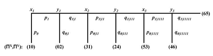
Figure 10.1: A truncated centipede game decision tree over 6 stages where two players $X$ and $Y$ alternately choose to either play down ($x_{i},y_{i}=0$ for $1\leq i\leq 3$) in which case the game stops, or play across ($x_{i},y_{i}=1$ for $1\leq i\leq 3$) so that either their opponent faces a similar choice or the game terminates in stage 6.

10.2 The centipede game

The centipede game gains its peculiar name as it normally features two players playing over 100 turns so that, when drawn horizontally as in Fig. 10.1, the game tree takes the appearance of a centipede. Here, we truncate the game without loss of generality at only 6 stages allowing a tractable analysis. In this truncated centipede game, each player $X$ or $Y$ must alternately elect to either play down ($x_{i},y_{i}=0$ for $1\leq i\leq 3$) in which case the game immediately terminates and players gain the respective payoffs shown, or play across ($x_{i},y_{i}=1$ for $1\leq i\leq 3$) in which case either their opponent plays or the game terminates with the payoffs shown. When either player hands play to their opponent, they suffer a short term loss of potential payoff with the prospect of a long term gain. The interest in this game comes from the countervailing effects of these short term losses and long term gains which combine together to ensure that human players typically fail to follow the recommendations of game theory and yet significantly improve their payoffs by doing so.

In fact, the centipede game has a unique subgame perfect equilibrium solution, which can be readily located by simply inspecting Fig. 10.1 and applying backwards induction. In the last (far right) stage, $Y$ can choose $y_{3}=0$ to obtain a payoff of $\Pi^{Y}=6$, or can choose $y_{3}=1$ to obtain a payoff of $\Pi^{Y}=5$. Obviously, $Y$ will prefer to play down with $y_{3}=0$ in this final stage to maximize their payoff. Player $X$ is well able to deduce this to conclude that if they choose $x_{3}=1$ to play across in the second last stage then they will obtain a payoff of $\Pi^{X}=4$ when $Y$ subsequently plays down. In contrast, should $X$ play down themselves by choosing $x_{3}=0$, they will gain the improved payoff of $\Pi^{X}=5$. Obviously, $X$ will choose $x_{3}=0$ to preempt $Y$’s choice of $y_{3}=0$. Exactly the same argument applies to $Y$’s choice in the fourth stage, to $X$’s choice in the third stage, to $Y$’s choice in the second stage, and finally to $X$’s choice in the first stage. That is, being able to deduce that $Y$ will play down in the second stage by choosing $y_{1}=0$ to give $X$ a payoff of $\Pi^{X}=0$, then player $X$ will choose to maximize their payoff by preempting $Y$ and playing down in the first stage through the choice $x_{1}=0$ to gain an improved payoff of $\Pi^{X}=1$. The associated payoff for $Y$ is $\Pi^{Y}=0$.

And here lies the conundrum. The sole conventionally mandated choice of play lies in the first player $X$ choosing down at the first opportunity to gain a mere fraction of the potential payoff should they and their opponent play across a few times. Interestingly, most people playing this game will indeed ignore the conventionally sanctioned choice with both players typically playing across repeatedly to drastically improve their payoffs. Just as in the other games under consideration here, it seems intuitively obvious to human players that adopting “non-rational” play will improve payoffs. However, conventional analysis has had trouble explaining these propensities. Here, we show that lifting implicit conventional bounds on rationality to allow players to take into account alternate probability spaces easily produces game theoretic predictions in agreement with observation.

Altogether, the payoffs to the players in the centipede game considered here are

$$\Pi^{X} = (1-x_{1})+x_{1}\left(y_{1}\left[3(1-x_{2})+x_{2}\left\{2(1-y_{2})+y_{2}\left(5(1-x_{3})+x_{3}\left[4(1-y_{3})+6y_{3}\right]\right)\right\}\right]\right)$$

$$\Pi^{Y} = x_{1}\left(2(1-y_{1})+y_{1}\left[1(1-x_{2})+x_{2}\left\{4(1-y_{2})+y_{2}\left(3(1-x_{3})+x_{3}\left[6(1-y_{3})+5y_{3}\right]\right)\right\}\right]\right).$$

As usual, players must then choose amongst their possible probability spaces ${\cal P}^{X}$ and ${\cal P}^{Y}$ to optimize their payoffs. A first choice will be the examination of the conventionally mandated probability space, which we turn to now.

10.2.1 The unconstrained space ${\cal P}^{X}_{B}\times{\cal P}^{Y}_{B}$

To replicate the standard conventional analysis (the backwards induction analysis above), both players $X$ and $Y$ together adopt a joint probability space ${\cal P}^{X}_{B}\times{\cal P}^{Y}_{B}$ in which every behavioural strategy on every history set is independent—see Figs. 10.1. The expected payoff optimization problem for each player $Z\in\{X,Y\}$ can be written

$$Z:\max\;\;\langle\Pi^{Z}\rangle = \sum_{x_{1},y_{1},x_{2},y_{2},x_{3},y_{3}=0}^{1}P^{XY}(x_{1},y_{1},x_{2},y_{2},x_{3},y_{3})\Pi^{Z}(x_{1},y_{1},x_{2},y_{2},x_{3},y_{3})$$

$$= \sum_{x_{1},y_{1},x_{2},y_{2},x_{3},y_{3}=0}^{1}P^{X}(x_{1})P^{Y}(y_{1}|x_{1})P^{X}(x_{2}|x_{1}y_{1})P^{Y}(y_{2}|x_{1}y_{1}x_{2})\times$$

$$\hskip 42.67912pt\times P^{X}(x_{3}|x_{1}y_{1}x_{2}y_{2})P^{Y}(y_{3}|x_{1}y_{1}x_{2}y_{2}x_{3})\Pi^{X}(x_{1},y_{1},x_{2},y_{2},x_{3},y_{3}).$$

To simplify notation, we write $P^{X}(x_{2}|x_{1}y_{1})\rightarrow p_{x_{2}|x_{1}y_{1}}$, $P^{Y}(y_{2}|x_{1}y_{1})\rightarrow q_{y_{2}|x_{1}y_{1}}$ and so on, and we take account of normalization conditions $p_{0|x_{1}y_{1}}+p_{1|x_{1}y_{1}}=1$ and $q_{0|x_{1}y_{1}}+q_{1|x_{1}y_{1}}=1$ on all histories.

Consequently, the expected payoff optimization problem becomes

$$X:\max_{p_{1},p_{1|11},p_{1|1111}}\;\;\langle\Pi^{X}\rangle = \left[1-p_{1}\right]+$$

$$\hskip 14.22636ptp_{1}\left\{0+\right.$$

$$\hskip 28.45274ptq_{1|1}\left(3\left[1-p_{1|11}\right]+\right.$$

$$\hskip 42.67912ptp_{1|11}\left\{2\left[1-q_{1|111}\right]+\right.$$

$$\hskip 56.9055ptq_{1|111}\left(5\left[1-p_{1|1111}\right]+\right.$$

$$\hskip 71.13188pt\left.\left.\left.\left.p_{1|1111}\left[4\left[1-q_{1|11111}\right]+6q_{1|11111}\right]\right)\right\}\right)\right\}$$

$$Y:\max_{q_{1|1},q_{1|111},q_{1|11111}}\;\;\langle\Pi^{Y}\rangle = p_{1}\left[2\left[1-q_{1|1}\right]+\right.$$ (10.3)

$$\hskip 14.22636ptq_{1|1}\left(\left[1-p_{1|11}\right]+\right.$$

$$\hskip 28.45274ptp_{1|11}\left\{4\left[1-q_{1|111}\right]+\right.$$

$$\hskip 42.67912ptq_{1|111}\left(3\left[1-p_{1|1111}\right]+\right.$$

$$\hskip 56.9055pt\left.\left.\left.\left.p_{1|1111}\left[6\left[1-q_{1|11111}\right]+5q_{1|11111}\right]\right)\right\}\right)\right].$$

In these optimization problems, the players $X$ and $Y$ have respective independent probability parameters of $p_{1},p_{1|11},p_{1|1111}$ and $q_{1|1},q_{1|111},q_{1|11111}$ all of which can vary freely over $[0,1]$. Consequently, in the joint space ${\cal P}^{X}_{B}\times{\cal P}^{Y}_{B}$, each player optimizes using the gradient operator

$$\nabla=\left[\frac{\partial}{\partial p_{1}},\frac{\partial}{\partial q_{1|1}},\frac{\partial}{\partial p_{1|11}},\frac{\partial}{\partial q_{1|111}},\frac{\partial}{\partial p_{1|1111}},\frac{\partial}{\partial q_{1|11111}}\right],$$ (10.4)

as all other parameters disappear. The easiest way to complete the optimization is via backwards induction, so both players first evaluate the last stage choice of player $Y$ via

$$\frac{\partial\langle\Pi^{Y}\rangle}{\partial q_{1|11111}}=-p_{1}q_{1|1}p_{1|11}q_{1|111}p_{1|1111}\leq 0,$$ (10.5)

which is either zero should any player have played down in any preceding stage in which case $Y$ is indifferent to any choice in this final stage, or always negative so essentially $Y$ plays down via $q_{1|11111}=0$ and $y_{3}=0$. This result allows player $X$ to optimize their choice in the second last stage via

$$\frac{\partial\langle\Pi^{X}\rangle}{\partial p_{1|1111}}=-p_{1}q_{1|1}p_{1|11}q_{1|111}\leq 0,$$ (10.6)

which again, leads to the setting $p_{1|1111}=0$ and $x_{3}=0$. A similar analysis proceeds backwards through all the stages to give the final solution, deducible by both players, of $(x_{1},y_{1},x_{2},y_{2},x_{3},y_{3})=(0,0,0,0,0,0)$. This choice garners players the conventionally mandated payoffs of $\left(\langle\Pi^{X}\rangle,\langle\Pi^{Y}\rangle\right)=(1,0)$.

10.2.2 Isomorphically constrained spaces

Naturally, players of unbounded rationality will not be content to merely examine the conventionally mandated joint probability space ${\cal P}^{X}_{B}\times{\cal P}^{Y}_{B}$ and will turn to consider alternative joint probability spaces. In each alternative space, isomorphic constraints alter game spaces and trees and thereby alter the subgame decompositions used in the conventional analysis to locate novel equilibria. We consider such alternatives now.

As usual, there are an infinity of possible probability spaces that might be adopted by the players in the sequential centipede game, and we can here consider only a partial search of these possible spaces. We first suppose that the players restrict their attention to “Markovian” strategies in which the variable of a given stage is only conditioned on the outcome of the immediately preceding stage. The alternative—correlating variables in the given stage to the outcomes in every preceding stage—simply generates to many options without adding significantly to the analysis. Given this restriction, a moments reflection will make it obvious that there is little point in a player choosing to anti-correlate their choice in a given stage to their opponent’s previous choice. There opponent must have played across so an anti-correlation would simply force a move down and this merely duplicate the outcomes of the conventional analysis above. The same considerations make it immediately attractive to have players consider perfect correlations between the opponent’s choices in the preceding stage and the current choices in the present stage as a previous choice of across then implies a current choice of across. We therefore suppose that players, in each stage after the first, can make their choices either independently or by correlation to their opponent’s previous choice.

These consideration leave four possible probability spaces to be enacted by player $X$, namely

$$\begin{array}[]{l}{\cal P}^{X}_{B}\\ {\cal P}^{X}_{B}|_{x_{2}=y_{1}}\\ {\cal P}^{X}_{B}|_{x_{3}=y_{2}}\\ {\cal P}^{X}_{B}|_{x_{2}=y_{1},x_{3}=y_{2}}.\end{array}$$ (10.7)

Similarly, there are eight possible spaces to be enacted by player $Y$, namely

$$\begin{array}[]{l}{\cal P}^{Y}_{B}\\ {\cal P}^{Y}_{B}|_{y_{1}=x_{1}}\\ {\cal P}^{Y}_{B}|_{y_{2}=x_{2}}\\ {\cal P}^{Y}_{B}|_{y_{3}=x_{3}}\\ {\cal P}^{Y}_{B}|_{y_{1}=x_{1},y_{2}=x_{2}}\\ {\cal P}^{Y}_{B}|_{y_{1}=x_{1},y_{3}=x_{3}}\\ {\cal P}^{Y}_{B}|_{y_{2}=x_{2},y_{3}=x_{3}}\\ {\cal P}^{Y}_{B}|_{y_{1}=x_{1},y_{2}=x_{2},y_{3}=x_{3}}.\end{array}$$ (10.8)

Altogether, this makes 32 joint probability spaces that need be considered. We now turn to follow the players in their analysis of the outcomes from their joint adoption of all of these combinations of spaces.

10.2.3 The space ${\cal P}^{X}_{B}|_{x_{2}=y_{1},x_{3}=y_{2}}\times{\cal P}^{Y}_{B}|_{y_{1}=x_{1},y_{2}=x_{2},y_{3}=x_{3}}$

Given the joint probability space ${\cal P}^{X}_{B}|_{x_{2}=y_{1},x_{3}=y_{2}}\times{\cal P}^{Y}_{B}|_{y_{1}=x_{1},y_{2}=x_{2},y_{3}=x_{3}}$ in which every variable after the first stage is isomorphically constrained to be perfectly correlated to the preceding choice by their opponent, we have the variable assignment reduces to $y_{3}=x_{3}=y_{2}=x_{2}=y_{1}=x_{1}$. Subsequently, the payoff functions for both players become

$$\Pi^{X} = (1-x_{1})+x_{1}\left(y_{1}\left[3(1-x_{2})+x_{2}\left\{2(1-y_{2})+y_{2}\left(5(1-x_{3})+x_{3}\left[4(1-y_{3})+6y_{3}\right]\right)\right\}\right]\right)$$

$$= (1-x_{1})+x_{1}\left(x_{1}\left[3(1-x_{1})+x_{1}\left\{2(1-x_{1})+x_{1}\left(5(1-x_{1})+x_{1}\left[4(1-x_{1})+6x_{1}\right]\right)\right\}\right]\right)$$

$$= 1+5x_{1}$$

$$\Pi^{Y} = x_{1}\left(2(1-y_{1})+y_{1}\left[1(1-x_{2})+x_{2}\left\{4(1-y_{2})+y_{2}\left(3(1-x_{3})+x_{3}\left[6(1-y_{3})+5y_{3}\right]\right)\right\}\right]\right).$$ (10.9)

$$= x_{1}\left(2(1-x_{1})+x_{1}\left[1(1-x_{1})+x_{1}\left\{4(1-x_{1})+x_{1}\left(3(1-x_{1})+x_{1}\left[6(1-x_{1})+5x_{1}\right]\right)\right\}\right]\right).$$

$$= 5x_{1}.$$

Here, it is immediately evident that player $X$ maximizes their payoff by setting $x_{1}=1$ generating a sequence of play of $(x_{1},x_{2},x_{3},y_{1},y_{2},y_{3})=(1,1,1,1,1,1)$ and payoffs of $(\Pi^{X},\Pi^{Y})=(6,5)$.

A similar result is obtained from optimizing the expected payoffs via

$$X:\max_{p_{1}}\;\;\langle\Pi^{X}\rangle = \sum_{x_{1},y_{1},x_{2},y_{2},x_{3},y_{3}=0}^{1}P^{X}(x_{1})\delta_{y_{1}x_{1}}\delta_{x_{2}y_{1}}\delta_{y_{2}x_{2}}\delta_{x_{3}y_{2}}\delta_{y_{3}x_{3}}\Pi^{X}$$

$$= \sum_{x_{1}=0}^{1}P^{X}(x_{1})\Pi^{X}(x_{1},x_{1},x_{1},x_{1},x_{1},x_{1})$$

$$= 1+5p_{1}$$

$$Y:\langle\Pi^{Y}\rangle = \sum_{x_{1},y_{1},x_{2},y_{2},x_{3},y_{3}=0}^{1}P^{X}(x_{1})\delta_{y_{1}x_{1}}\delta_{x_{2}y_{1}}\delta_{y_{2}x_{2}}\delta_{x_{3}y_{2}}\delta_{y_{3}x_{3}}\Pi^{Y}$$ (10.10)

$$= \sum_{x_{1}=0}^{1}P^{X}(x_{1})\Pi^{Y}(x_{1},x_{1},x_{1},x_{1},x_{1},x_{1})$$

$$= 5p_{1}.$$

Here, player $Y$ has left themselves no choices in any stage. As a result, the optimization is completed by

$$\frac{\partial\langle\Pi^{X}\rangle}{\partial p_{1}}=5>0,$$ (10.11)

so $X$ sets $p_{1}=1$ to choose $x_{1}=1$ and plays across in stage 1. This choice is mimicked in every subsequent stage giving $(x_{1},y_{1},x_{2},y_{2},x_{3},y_{3})=(1,1,1,1,1,1)$ to generate payoffs to the players of $\left(\langle\Pi^{X}\rangle,\langle\Pi^{Y}\rangle\right)=(6,5)$.

10.2.4 The space ${\cal P}^{X}_{B}|_{x_{2}=y_{1},x_{3}=y_{2}}\times{\cal P}^{Y}_{B}|_{y_{2}=x_{2},y_{3}=x_{3}}$

In the joint probability space ${\cal P}^{X}_{B}|_{x_{2}=y_{1},x_{3}=y_{2}}\times{\cal P}^{Y}_{B}|_{y_{2}=x_{2},y_{3}=x_{3}}$ the variable assignment reduces to $y_{3}=x_{3}=y_{2}=x_{2}=y_{1}$ so the payoff functions become

$$\Pi^{X} = (1-x_{1})+x_{1}\left(y_{1}\left[3(1-x_{2})+x_{2}\left\{2(1-y_{2})+y_{2}\left(5(1-x_{3})+x_{3}\left[4(1-y_{3})+6y_{3}\right]\right)\right\}\right]\right)$$

$$= (1-x_{1})+x_{1}\left(y_{1}\left[3(1-y_{1})+y_{1}\left\{2(1-y_{1})+y_{1}\left(5(1-y_{1})+y_{1}\left[4(1-y_{1})+6y_{1}\right]\right)\right\}\right]\right)$$

$$= 1-x_{1}+6x_{1}y_{1}$$

$$\Pi^{Y} = x_{1}\left(2(1-y_{1})+y_{1}\left[1(1-x_{2})+x_{2}\left\{4(1-y_{2})+y_{2}\left(3(1-x_{3})+x_{3}\left[6(1-y_{3})+5y_{3}\right]\right)\right\}\right]\right)$$ (10.12)

$$= x_{1}(2+3y_{1}).$$

These payoff functions establish that player $Y$ maximizes their payoff by setting $y_{1}=1$ while player $X$ maximizes their income by setting $x_{1}=1$ generating a sequence of play of $(x_{1},x_{2},x_{3},y_{1},y_{2},y_{3})=(1,1,1,1,1,1)$ and payoffs of $(\Pi^{X},\Pi^{Y})=(6,5)$.

The expected payoff functions optimization task becomes

$$X:\max_{p_{1}}\;\;\langle\Pi^{X}\rangle = \sum_{x_{1},y_{1},x_{2},y_{2},x_{3},y_{3}=0}^{1}P^{X}(x_{1})P^{Y}(y_{1}|x_{1})\delta_{x_{2}y_{1}}\delta_{y_{2}x_{2}}\delta_{x_{3}y_{2}}\delta_{y_{3}x_{3}}\Pi^{X}$$

$$= \sum_{x_{1}y_{1}=0}^{1}P^{X}(x_{1})P^{Y}(y_{1}|x_{1})\Pi^{X}(x_{1},y_{1},y_{1},y_{1},y_{1},y_{1})$$

$$= 1-p_{1}+6p_{1}q_{1|1}$$

$$Y:\max_{q_{1|1}}\;\;\langle\Pi^{Y}\rangle = \sum_{x_{1},y_{1},x_{2},y_{2},x_{3},y_{3}=0}^{1}P^{X}(x_{1})P^{Y}(y_{1}|x_{1})\delta_{x_{2}y_{1}}\delta_{y_{2}x_{2}}\delta_{x_{3}y_{2}}\delta_{y_{3}x_{3}}\Pi^{Y}$$ (10.13)

$$= \sum_{x_{1}y_{1}=0}^{1}P^{X}(x_{1})P^{Y}(y_{1}|x_{1})\Pi^{Y}(x_{1},y_{1},y_{1},y_{1},y_{1},y_{1})$$

$$= p_{1}\left[2+3q_{1|1}\right].$$

In this case, the optimization is completed by

$$\frac{\partial\langle\Pi^{X}\rangle}{\partial p_{1}} = -1+6q_{1|1}$$

$$\frac{\partial\langle\Pi^{Y}\rangle}{\partial q_{1|1}} = 3p_{1}.$$ (10.14)

Essentially then, player $Y$ notes their positive gradient and so sets $q_{1|1}=1$ to give $y_{1}=1$. In turn, player $X$ deduces this and sets $p_{1}=1$ to give $x_{1}=1$. Together, in the joint probability space ${\cal P}^{X}_{B}|_{x_{2}=y_{1},x_{3}=y_{2}}\times{\cal P}^{Y}_{B}|_{y_{2}=x_{2},y_{3}=x_{3}}$, the optimization generates the play choices $(x_{1},y_{1},x_{2},y_{2},x_{3},y_{3})=(1,1,1,1,1,1)$ to generate payoffs to the players of $\left(\langle\Pi^{X}\rangle,\langle\Pi^{Y}\rangle\right)=(6,5)$.

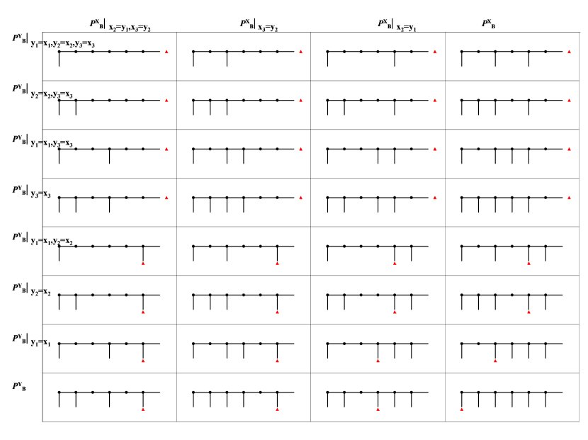
Figure 10.2: The 32 distinct trees and equilibrium pathways (indicated by triangles) given that players $X$ and $Y$ adopt the probability spaces shown. Dots indicate successive decision nodes, where nodes with a descending vertical line are independent decision points and nodes lacking a descending vertical line are isomorphically constrained to equal the immediately preceding decision.

10.2.5 Expected payoff comparison across multiple probability spaces

Similar analysis to that above can be applied to evaluate the expected payoffs in all the other combinations of joint probability spaces to give the payoff combination table

$$\begin{array}[]{c|cccc}\left(\langle\Pi^{X}\rangle,\langle\Pi^{Y}\rangle\right)&{\cal P}^{X}_{B}|_{x_{2}=y_{1},x_{3}=y_{2}}&{\cal P}^{X}_{B}|_{x_{3}=y_{2}}&{\cal P}^{X}_{B}|_{x_{2}=y_{1}}&{\cal P}^{X}_{B}\\ \hline\cr{\cal P}^{Y}_{B}|_{y_{1}=x_{1},y_{2}=x_{2},y_{3}=x_{3}}&(6,5)&(6,5)&(6,5)&(6,5)\\ {\cal P}^{Y}_{B}|_{y_{1}=x_{1},y_{3}=x_{3}}&(6,5)&(6,5)&(6,5)&(6,5)\\ {\cal P}^{Y}_{B}|_{y_{2}=x_{2},y_{3}=x_{3}}&(6,5)&(6,5)&(6,5)&(6,5)\\ {\cal P}^{Y}_{B}|_{y_{3}=x_{3}}&(6,5)&(6,5)&(6,5)&(6,5)\\ {\cal P}^{Y}_{B}|_{y_{1}=x_{1},y_{2}=x_{2}}&(4,6)&(4,6)&(5,3)&(5,3)\\ {\cal P}^{Y}_{B}|_{y_{1}=x_{1}}&(4,6)&(4,6)&(5,3)&(5,3)\\ {\cal P}^{Y}_{B}|_{y_{2}=x_{2}}&(4,6)&(4,6)&(2,4)&(3,1)\\ {\cal P}^{Y}_{B}&(4,6)&(4,6)&(2,4)&(1,0).\\ \end{array}.$$ (10.15)

The equivalent trees and equilibrium pathways are shown in Fig. 10.2. Perusal of this table makes it clear that players do not optimize their payoffs by choosing the conventionally mandated joint probability space. Rather, it is much more likely that $Y$ will choose any probability space in which their last stage variable is isomorphically constrained. In turn, this alters the payoffs for player $X$ in such a way as to render them indifferent to any choice of probability space. The net result will be that $X$ will find themselves playing across in the first stage irrespective of which space they adopt.

A more sophisticated analysis in a longer game would take into account end-game effects where players might express some preference for terminating the game slightly early. Such tendencies are similar to those seen in the finite iterated prisoner’s dilemma game, and as there, are not likely to make it irrational for players to play across in the early stages of the centipede game.

The extended analysis presented here produces game theoretic predictions in substantial accord with observed human play in the centipede game. As noted above, this agreement contrasts sharply with the manifest contradiction between the game theoretic predictions of conventional analysis and observed play tendencies. As such, we take these observations as evidence that humans naturally take account of isomorphic constraints in strategic play in game theory.

Chapter 11 The Iterated Prisoner’s Dilemma

11.1 Introduction

Conventional game analysis holds that it is rational for players in a finite iterated prisoner’s dilemma to adopt the noncooperative “all defect” as the optimal solution under common knowledge of rationality (CKR) even though human players are commonly observed to increase payoffs by irrationally adopting alternative strategies. There are many observations of this mismatch between theoretical prediction and observed behaviour [96, 97, 98, 99]. These mismatches have typically been explained by introducing behavioral factors such as bounded rationality, incomplete information, and other innate tendencies promoting cooperative and altruistic behaviours. In particular, these suggestions include modifying definitions of rationality to include reciprocity, fairness and altruism or to otherwise bound rationality [100, 101, 102, 103, 104, 64, 105], via modelling the evolution of cooperation [106, 77], by taking account of incomplete information [107, 108, 109, 110] and uncertainty in the number of repeat stages [111], to bound the complexity of implementable strategies [112, 113, 114], to account for communication and coordination costs [115], to incorporate reputation and experimentation effects [116] or secondary utility functions as in benevolence theory [25] or in moral discussions [117], to include adaptive learning [118] or fuzzy logic [119], or more directly, to employ comprehensive constructions of normal form strategy tables incorporating belief strategies [120, 121, 122]. Interestingly, quantum correlations can be introduced to resolve the prisoner’s dilemma [123].

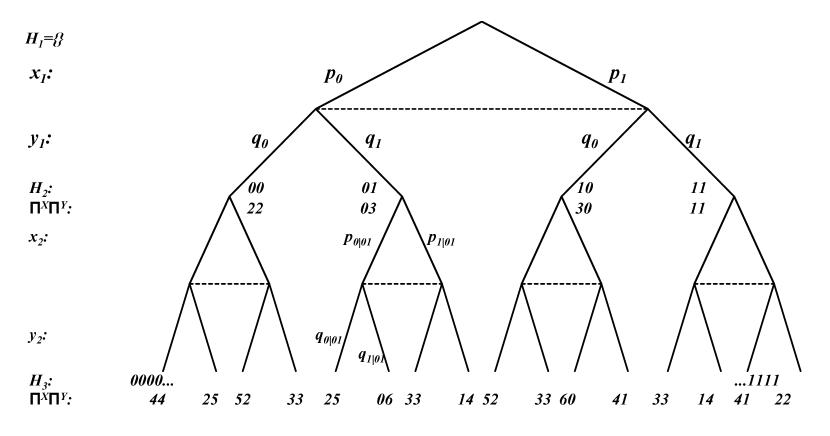
Figure 11.1: A two stage game decision tree where two non-communicating players simultaneously choose moves $x_{n}$ or $y_{n}$ equal to “0” or “1” at stage $n$ with respective probabilities $P^{X}(x_{n}|H_{n})$ and $P^{Y}(y_{n}|H_{n})$ at every decision point. At the beginning of each stage, players know the history sets $H_{n}=\{x_{1},y_{1},\dots,x_{n-1},y_{n-1}\}$ detailing the shared information known to both players of all choices to that stage (with $H_{1}=\{\}$). Players also know their cumulative payoffs $(\Pi^{X},\Pi^{Y})$ to that point.

11.2 The finite Iterated Prisoner’s Dilemma

In this chapter, we will examine the finite iterated prisoner’s dilemma while using the strong isomorphic mappings of probability theory to construct our mixed and behavioural strategy game spaces. Our particular focus will be to examine whether cooperation is rational in the finite iterated prisoner’s dilemma. As usual, we assume our players are rational and of unbounded capacity, and that they have adopted common knowledge of rationality (CKR). An illustrative game tree depicting a two stage iterated prisoner’s dilemma is shown in Fig. 11.1.

The finite iterated prisoner’s dilemma is defined here over a finite number of $N$ stages, where at each stage $1\leq n\leq N$ two non-communicating players $X$ and $Y$ choose moves $x_{n}$ and $y_{n}$ chosen to be either $0$ (cooperation) or $1$ (defection). The payoffs gained in each stage are given by the payoff matrix

$$\begin{array}[]{cc}&Y\\ X&\begin{array}[]{c|cc}(\pi_{x},\pi_{y})&0&1\\ \hline\cr 0&(2,2)&(0,3)\\ 1&(3,0)&(1,1),\\ \end{array}\end{array}$$ (11.1)

equivalent to the single stage payoff functions

$$\pi_{x}(x_{n},y_{n}) = 2+x_{n}-2y_{n}$$

$$\pi_{y}(x_{n},y_{n}) = 2-2x_{n}+y_{n}.$$ (11.2)

For multiple stage games, total game payoffs of a finite $N$ stage game are simply the sum of single stage payoffs. The optimization problem for both players is then

$$X:\max_{x_{1},\dots,x_{N}}\;\;\Pi^{X}(x_{1},y_{1},\dots x_{N},y_{N}) = \sum_{n=1}^{N}(2+x_{n}-2y_{n})$$

$$Y:\max_{y_{1},\dots,y_{N}}\;\;\Pi^{Y}(x_{1},y_{1},\dots x_{N},y_{N}) = \sum_{n=1}^{N}(2-2x_{n}+y_{n}).$$ (11.3)

Each player desires to maximize their respective endgame payoffs by varying their respective move choices $x_{n}$ and $y_{n}$ over every stage of the game. (The players know $N$ in advance.)

Yet more generally, players choose their moves probabilistically to prevent their opponent predicting and exploiting deterministic strategies. The players will then adopt the joint probability space ${\cal P}^{X}\times{\cal P}^{Y}$, and so seek to maximize their respective expected payoffs

$$X:\max_{{\cal P}^{X}}\;\;\langle\Pi^{X}\rangle = \sum_{x_{1}\dots y_{N}=0}^{1}P^{XY}(x_{1},y_{1},\dots,x_{N},y_{N})\Pi^{X}(x_{1},y_{1},\dots,x_{N},y_{N})$$

$$= \sum_{x_{1}\dots y_{N}=0}^{1}P^{X}(x_{1})P^{Y}(y_{1})P^{X}(x_{2}|H_{2})P^{Y}(y_{2}|H_{2})\dots\times$$

$$\hskip 56.9055pt\dots P^{X}(x_{N}|H_{N})P^{Y}(y_{N}|H_{N})\sum_{n=1}^{N}(2+x_{n}-2y_{n})$$

$$= 2N+\sum_{n=1}^{N}\sum_{\stackrel{{\scriptstyle x_{1}\dots x_{n}=0}}{{y_{1}\dots y_{n}=0}}}^{1}P^{X}(x_{1})P^{Y}(y_{1})P^{X}(x_{2}|H_{2})P^{Y}(y_{2}|H_{2})\dots\times$$

$$\hskip 85.35826pt\dots P^{X}(x_{n}|H_{n})P^{Y}(y_{n}|H_{n})(x_{n}-2y_{n})$$

$$Y:\max_{{\cal P}^{Y}}\;\;\langle\Pi^{Y}\rangle = \sum_{x_{1}\dots y_{N}=0}^{1}P^{XY}(x_{1},y_{1},\dots,x_{N},y_{N})\Pi^{Y}(x_{1},y_{1},\dots,x_{N},y_{N})$$ (11.4)

$$= \sum_{x_{1}\dots y_{N}=0}^{1}P^{X}(x_{1})P^{Y}(y_{1})P^{X}(x_{2}|H_{2})P^{Y}(y_{2}|H_{2})\dots\times$$

$$\hskip 56.9055pt\dots P^{X}(x_{N}|H_{N})P^{Y}(y_{N}|H_{N})\sum_{n=1}^{N}(2-2x_{n}+y_{n})$$

$$= 2N+\sum_{n=1}^{N}\sum_{\stackrel{{\scriptstyle x_{1}\dots x_{n}=0}}{{y_{1}\dots y_{n}=0}}}^{1}P^{X}(x_{1})P^{Y}(y_{1})P^{X}(x_{2}|H_{2})P^{Y}(y_{2}|H_{2})\dots\times$$

$$\hskip 85.35826pt\dots P^{X}(x_{n}|H_{n})P^{Y}(y_{n}|H_{n})(y_{n}-2x_{n}),$$

We have written $P^{Z}(z_{n}|H_{n})$ as the conditioned probability distribution at stage $n$ that player $Z$ chooses move $z_{n}$ (either $x_{n}$ or $y_{n}$) given history $H_{n}=\{x_{1},y_{1},\dots,x_{n-1},y_{n-1}\}$ detailing the shared information known to both players of all choices to that stage (with $H_{1}=\{\}$). We further write $P^{X}(x_{1}|H_{1})=P^{X}(x_{1})=p_{1}$, $P^{Y}(y_{1}|H_{1})=P^{Y}(y_{1})=q_{1}$, $P^{X}(x_{n}|H_{n})=p_{x_{n}|H_{n}}$ and $P^{Y}(y_{n}|H_{n})=q_{y_{n}|H_{n}}$. The expected payoffs are obtained by summing over every possible path through the game tree specified by the move choices $x_{1},y_{1},\dots,x_{N},y_{N}$, with each path weighted by the joint probability of that path being selected $P^{XY}(x_{1},y_{1},\dots,x_{N},y_{N})$, and where each path generates a payoff of $\Pi^{Z}(x_{1},y_{1},\dots,x_{N},y_{N})$ for player $Z$.

Here, as usual, the players $X$ and $Y$ vary their choice of respective probability space ${\cal P}^{X}$ and ${\cal P}^{Y}$ so as to maximize their expected payoff. That is, we hold that such players will avail themselves of the strong isomorphic mappings adopted by probability theory to construct their mixed or behavioural strategy spaces. Hence, each player will sequentially analyze situations where both players adopt altered joint probability spaces ${\cal P}^{X}_{i}\times{\cal P}^{Y}_{j}$ for $i,j=0,1,2,\dots$. The infinity of possible alternatives mandates that some limits be placed on the search space.

In the following analysis, we will first consider the $N=1$ single stage prisoner dilemma game. This will inform our subsequent analysis of the $N=2$ stage prisoner’s dilemma. We will analyze the $N=2$ stage game by comparing three strategies commonly found in the literature—conventional independent play, a Tit-For-Tat strategy, and All Defect—with a functionally correlated Markovian probability strategy space. This analysis will then be generalized to consider a total of 256 alternate joint probability spaces. Finally, we will consider a multiple stage game with $N$ arbitrary and analyze a number of alternate joint probability spaces.

11.3 The $N=1$ stage Prisoner’s dilemma

The single stage prisoner’s dilemma has the players seeking to optimize the payoff functions

$$X:\max_{x_{1}}\;\;\Pi^{X}(x_{1},y_{1}) = 2+x_{1}-2y_{1}$$

$$Y:\max_{y_{1}}\;\;\Pi^{Y}(x_{1},y_{1}) = 2-2x_{1}+y_{1}.$$ (11.5)

We suppose that players adopt a joint behavioural probability space ${\cal P}^{X}_{B}\times{\cal P}^{X}_{B}$. Because of the lack of communication, the choices of the $x_{1}$ and $y_{1}$ variables are independent. One possible joint probability space defines the expected payoff optimization problem for each player as

$$X:\max_{p_{1}}\;\;\langle\Pi^{X}\rangle = \sum_{x_{1}y_{1}=0}^{1}P^{XY}(x_{1},y_{1})\Pi^{X}(x_{1},y_{1})$$

$$= \sum_{x_{1}y_{1}=0}^{1}P^{X}(x_{1})P^{Y}(y_{1})(2+x_{1}-2y_{1})$$

$$= 2+p_{1}-2q_{1}$$

$$Y:\max_{q_{1}}\;\;\langle\Pi^{Y}\rangle = \sum_{x_{1}y_{1}=0}^{1}P^{XY}(x_{1},y_{1})\Pi^{Y}(x_{1},y_{1})$$ (11.6)

$$= \sum_{x_{1}y_{1}=0}^{1}P^{X}(x_{1})P^{Y}(y_{1})(2-2x_{1}+y_{1})$$

$$= 2-2p_{1}+q_{1},$$

where use has been made of the normalization conditions $p_{0}+p_{1}=1$ and $q_{0}+q_{1}=1$. In this two-player-single-stage game, each expected payoff function is a function of the independent parameters $p_{1}$ and $q_{1}$ and so are maximized by the gradient operator

$$\nabla=\left[\frac{\partial}{\partial p_{1}},\frac{\partial}{\partial q_{1}}\right],$$ (11.7)

giving the joint optimization conditions

$$\frac{\partial\langle\Pi^{X}\rangle}{\partial p_{1}} = 1$$

$$\frac{\partial\langle\Pi^{Y}\rangle}{\partial q_{1}} = 1.$$ (11.8)

Together, these make it evident that each player optimizes their expected payoff by maximizing their defection probability (choosing $p_{1}=1$ and $q_{1}=1$) irrespective of their opponent’s choices. That is, both players defect with certainty. This is the unique single-stage Nash equilibrium point [3] from which neither player can unilaterally alter their choice without worsening their payoff. Even so, payoffs are jointly maximized when both players cooperate (via $x_{1}=y_{1}=0$) to yield payoffs of $(\Pi^{X},\Pi^{Y})=(2,2)$. Herein lies the dilemma.

We now turn to consider the $N=2$ stage iterated prisoner’s dilemma.

11.4 The $N=2$ stage prisoner’s dilemma

For the $N=2$ stage game, the optimization problem for both players is

$$X:\max_{x_{1},x_{2}}\;\;\Pi^{X} = \sum_{n=1}^{2}(2+x_{n}-2y_{n})$$

$$Y:\max_{y_{1},y_{2}}\;\;\Pi^{Y} = \sum_{n=1}^{2}(2-2x_{n}+y_{n}).$$ (11.9)

The question which needs to be addressed by each player is how to take account of all of the possible functional relationships that might exist between the variables. Of course, when the variables are functionally related then this imposes constraints onto the calculation of gradients which effects optimization outcomes. Game theory presumes there exists a single space which properly takes into account every possible functional dependency. Probability theory and optimization theory in general hold that no such single space exists. These fields employ a multiplicity of distinct spaces in order to take account of the different possible dependencies. In what follows, we will consider a small number of different possible functional dependencies.

11.4.1 The unconstrained space ${\cal P}^{X}_{B}\times{\cal P}^{Y}_{B}$

Conventional game analysis assumes that rational players $X$ and $Y$ will adopt a single specific joint probability space, denoted here ${\cal P}^{X}_{B}\times{\cal P}^{Y}_{B}$. In this space, the absence of isomorphism constraints means that all behavioural strategies are independent allowing the game to be decomposed into subgames in every history separating the last stage from the preceding stage. Then, optimization in the last stage is independent of both prior and non-existent future events, so the last stage is identically a single stage game and optimized in the prisoner’s dilemma via the unique single stage Nash equilibria of mutual defection. This process can then be iterated backwards through the game (backwards induction) to locate the unique Nash equilibria for the entire game of mutual defection in every stage. We now detail this analysis.

In the space ${\cal P}^{X}_{B}\times{\cal P}^{Y}_{B}$, players seek to optimize their respective expected payoffs

$$X:\max\;\;\langle\Pi^{X}\rangle = 2N+\sum_{n=1}^{2}\sum_{x_{1}\dots y_{n}=0}^{1}P^{X}(x_{1})P^{Y}(y_{1})\dots P^{X}(x_{n}|H_{n})P^{Y}(y_{n}|H_{n})(x_{n}-2y_{n})$$

$$= 4+p_{1}-2q_{1}+\left[1-p_{1}\right]\left[1-q_{1}\right]\left[p_{1|00}-2q_{1|00}\right]$$

$$+\left[1-p_{1}\right]q_{1}\left[p_{1|01}-2q_{1|01}\right]$$

$$+p_{1}\left[1-q_{1}\right]\left[p_{1|10}-2q_{1|10}\right]+p_{1}q_{1}\left[p_{1|11}-2q_{1|11}\right]$$

$$Y:\max\;\;\langle\Pi^{Y}\rangle = 2N+\sum_{n=1}^{2}\sum_{x_{1}\dots y_{n}=0}^{1}P^{X}(x_{1})P^{Y}(y_{1})\dots P^{X}(x_{n}|H_{n})P^{Y}(y_{n}|H_{n})(y_{n}-2x_{n})$$ (11.10)

$$= 4-2p_{1}+q_{1}+\left[1-p_{1}\right]\left[1-q_{1}\right]\left[q_{1|00}-2p_{1|00}\right]$$

$$+\left[1-p_{1}\right]q_{1}\left[q_{1|01}-2p_{1|01}\right]$$

$$+p_{1}\left[1-q_{1}\right]\left[q_{1|10}-2p_{1|10}\right]+p_{1}q_{1}\left[q_{1|11}-2p_{1|11}\right].$$

These expected payoff functions can take account of every possible state of correlation between the second stage variables $x_{2}$ and $y_{2}$ and the first stage variables $x_{1}$ and $y_{1}$. The first stage probability variables $p_{1},q_{1}$, together with the second stage variables $p_{1|00},p_{1|01},p_{1|10},p_{1|11}$, and $q_{1|00},q_{1|01},q_{1|10},q_{1|11}$ are all freely varying over the range $[0,1]$. As a result, the relevant gradient operator used by both players to analyze this particular probability space is

$$\nabla = \left[\frac{\partial}{\partial p_{1}},\frac{\partial}{\partial q_{1}},\frac{\partial}{\partial p_{1|00}},\frac{\partial}{\partial p_{1|01}},\frac{\partial}{\partial p_{1|10}},\frac{\partial}{\partial p_{1|11}},\frac{\partial}{\partial q_{1|00}},\frac{\partial}{\partial q_{1|01}},\frac{\partial}{\partial q_{1|10}},\frac{\partial}{\partial q_{1|11}}\right].$$ (11.11)

Immediately then, optimization with respect to second stage variables by player $X$ gives

$$\frac{\partial\langle\Pi^{X}\rangle}{\partial p_{1|00}} = \left[1-p_{1}\right]\left[1-q_{1}\right]\geq 0$$

$$\frac{\partial\langle\Pi^{X}\rangle}{\partial p_{1|01}} = \left[1-p_{1}\right]q_{1}\geq 0$$

$$\frac{\partial\langle\Pi^{X}\rangle}{\partial p_{1|10}} = p_{1}\left[1-q_{1}\right]\geq 0$$

$$\frac{\partial\langle\Pi^{X}\rangle}{\partial p_{1|11}} = p_{1}q_{1}\geq 0,$$ (11.12)

with similar results applying for $Y$. As the rate of change of the expected payoff is essentially positive with increasing last stage defection probability, each player maximizes their expected payoff by defecting with certainty in the last stage. That is, each player sets $p_{1|x_{1}y_{1}}=1$ and $q_{1|x_{1}y_{1}}=1$ on every pathway. Taking account of this last stage result simplifies the optimization for the first stage probability variables (backwards induction), giving

$$\frac{\partial\langle\Pi^{X}\rangle}{\partial p_{1}}=1,$$ (11.13)

with similar results applying for $Y$. Again, players will defect in the first stage by setting $p_{1}=1$ and $q_{1}=1$. Hence, players conclude that, given the adoption of the joint probability space ${\cal P}^{X}_{B}\times{\cal P}^{Y}_{B}$, they maximize their expected payoffs by defecting in every stage of the game $(x_{1},y_{1},x_{2},y_{2})=(1,1,1,1)$ to derive a joint expected payoff of $\left(\langle\Pi^{X}\rangle,\langle\Pi^{Y}\rangle\right)=(N,N)=(2,2)$. This is the unique Nash equilibrium pathway for the finite iterated prisoner’s dilemma, given the adoption of the joint probability space ${\cal P}^{X}_{B}\times{\cal P}^{Y}_{B}$.

11.4.2 Alternate isomorphic probability spaces

In this section we suppose that players $X$ and $Y$ consider only a choice of four possible alternate probability spaces, namely, the conventional independent behavioural strategy space, a functionally correlated Markovian probability space, a Tit-For-Tat strategy space, and an All Defect strategy space.

When adopting a Markovian space, each player functionally correlates their second stage choices to their opponent’s first stage choices. That is, player $X$ implements

$$x_{2} = y_{1}$$

$$p_{x_{2}|x_{1}y_{1}} = \delta_{x_{2}y_{1}},$$ (11.14)

while player $Y$ chooses

$$y_{2} = x_{1}$$

$$q_{y_{2}|x_{1}y_{1}} = \delta_{y_{2}x_{1}}.$$ (11.15)

We denote these spaces respectively as ${\cal P}^{X}_{B}|_{x_{2}=y_{1}}$ and ${\cal P}^{Y}_{B}|_{y_{2}=x_{1}}$.

When adopting Tit-For-Tat, each player chooses to cooperate in the first stage and then functionally correlate their second stage choice to the opponent’s first stage choice. Player $X$ implements Tit-For-Tat via

$$x_{1} = 0$$

$$p_{x_{1}} = \delta_{x_{1}0}$$

$$x_{2} = y_{1}$$

$$p_{x_{2}|x_{1}y_{1}} = \delta_{x_{2}y_{1}},$$ (11.16)

while player $Y$ will implement

$$y_{1} = 0$$

$$q_{y_{1}} = \delta_{y_{1}0}$$

$$y_{2} = x_{1}$$

$$q_{y_{2}|x_{1}y_{1}} = \delta_{y_{2}x_{1}}.$$ (11.17)

We denote these probability spaces respectively as ${\cal P}^{X}_{B}|_{x_{1}=0,x_{2}=y_{1}}$ and ${\cal P}^{Y}_{B}|_{y_{1}=0,y_{2}=x_{1}}$.

Finally, by adopting the ALL DEFECT space, each player chooses to defect in every stage. Player $X$ chooses

$$x_{1} = 1$$

$$p_{x_{1}} = \delta_{x_{1}1}$$

$$x_{2} = 1$$

$$p_{x_{2}|x_{1}y_{1}} = \delta_{x_{2}1},$$ (11.18)

and player $Y$ chooses

$$y_{1} = 1$$

$$q_{y_{1}} = \delta_{y_{1}1}$$

$$y_{2} = 1$$

$$q_{y_{2}|x_{1}y_{1}} = \delta_{y_{2}1}.$$ (11.19)

We denote these probability spaces respectively as ${\cal P}^{X}_{B}|_{x_{1}=x_{2}=1}$ and ${\cal P}^{Y}_{B}|_{y_{1}=y_{2}=1}$.

Subsequently, players of unbounded rationality will then sequentially examine the alternate isomorphic probability spaces available to the players. Within each possible space, they will locate the constrained equilibria optimizing outcomes, and then later compare these outcomes in a comparison table. We complete this process now.

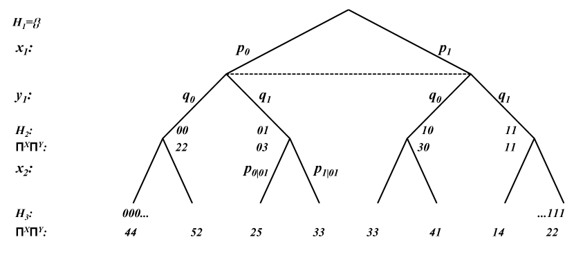
Figure 11.2: The case where players $(X,Y)$ adopt Independent versus Markovian strategies in the ${\cal P}^{X}_{B}\times{\cal P}^{Y}_{B}|_{y_{2}=x_{1}}$ joint probability space. The second stage choices of player $Y$ are isomorphically constrained and so are not freely varying parameters and do not appear in the decision tree.

11.4.3 $N=2$ stage: Independent versus Markovian strategies

Supposing that the players examine the case where they adopt Independent versus Markovian strategies and so jointly adopt the ${\cal P}^{X}_{B}\times{\cal P}^{Y}_{B}|_{y_{2}=x_{1}}$ probability space. In this space, the players seek to optimize (11.4.1) subject to the isomorphic constraint $y_{2}=x_{1}$. This constraint alters the expected payoff optimization problems to be

$$X:\max_{p_{1},p_{1|x_{1}y_{1}}}\;\;\langle\Pi^{X}\rangle = 4+p_{1}-2q_{1}+$$

$$\left[1-p_{1}\right]\left[1-q_{1}\right]p_{1|00}+$$

$$\left[1-p_{1}\right]q_{1}p_{1|01}+$$

$$p_{1}\left[1-q_{1}\right]\left[p_{1|10}-2\right]+$$

$$p_{1}q_{1}\left[p_{1|11}-2\right]$$

$$Y:\max_{q_{1}}\;\;\langle\Pi^{Y}\rangle = 4-2p_{1}+q_{1}+$$ (11.20)

$$-2\left[1-p_{1}\right]\left[1-q_{1}\right]p_{1|00}-$$

$$2\left[1-p_{1}\right]q_{1}p_{1|01}+$$

$$p_{1}\left[1-q_{1}\right]\left[1-2p_{1|10}\right]+$$

$$p_{1}q_{1}\left[1-2p_{1|11}\right].$$

These expected payoffs are continuous multivariate functions dependent only on the freely varying parameters $[p_{1},q_{1},p_{1|00},p_{1|01},p_{1|10},p_{1|11}]$. Consequently, the relevant gradient operator used by both players to analyze this particular probability space is

$$\nabla = \left[\frac{\partial}{\partial p_{1}},\frac{\partial}{\partial q_{1}},\frac{\partial}{\partial p_{1|00}},\frac{\partial}{\partial p_{1|01}},\frac{\partial}{\partial p_{1|10}},\frac{\partial}{\partial p_{1|11}}\right]$$

while the resulting game tree is shown in Fig. 11.2. Optimization then proceeds as usual via

$$\frac{\partial\langle\Pi^{X}\rangle}{\partial p_{1|00}} = \left[1-p_{1}\right]\left[1-q_{1}\right]\geq 0$$

$$\frac{\partial\langle\Pi^{X}\rangle}{\partial p_{1|01}} = \left[1-p_{1}\right]q_{1}\geq 0$$

$$\frac{\partial\langle\Pi^{X}\rangle}{\partial p_{1|10}} = p_{1}\left[1-q_{1}\right]\geq 0$$

$$\frac{\partial\langle\Pi^{X}\rangle}{\partial p_{1|11}} = p_{1}q_{1}\geq 0,$$ (11.22)

ensuring that player $X$ defects with certainty in the last stage by setting $p_{1|x_{1}y_{1}}=1$ on every pathway. These choices then allow evaluating

$$X:\max_{p_{1}}\;\;\langle\Pi^{X}\rangle = 5-p_{1}-2q_{1}$$

$$\frac{\partial\langle\Pi^{X}\rangle}{\partial p_{1}} = -1\leq 0,$$ (11.23)

so player $X$ cooperates with certainty in the first stage by setting $p_{1}=0$. In contrast, the analysis by player $Y$ must simply determine their first stage variable (taking account of the optimized moves by player $X$) via

$$Y:\max_{q_{1}}\;\;\langle\Pi^{Y}\rangle = 2+2q_{1}$$

$$\frac{\partial\langle\Pi^{Y}\rangle}{\partial q_{1}} = 1\geq 0,$$ (11.24)

so player $Y$ defects in the first stage by setting $q_{1}=1$. Altogether, when players $(X,Y)$ adopt the ${\cal P}^{X}_{B}\times{\cal P}^{Y}_{B}|_{y_{2}=x_{1}}$ joint probability space, they play the move combinations $(x_{1},y_{1},x_{2},y_{2})=(0,1,1,0)$ to garner payoffs $\left(\langle\Pi^{X}\rangle,\langle\Pi^{Y}\rangle\right)=(3,3)$. Here, in this particular joint probability space, the player adopting an Independent strategy must cooperate in the first stage to ensure that their mimicking opponent playing a Markovian will cooperate in the second stage so setting them up for a sucker’s payoff in that stage. However, this gains them little as their opponent can still freely defect in the first stage so in the end, players end up with equal payoffs.

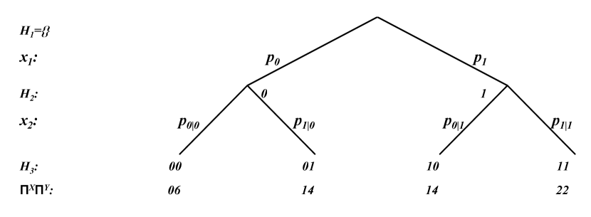
Figure 11.3: The case where players $(X,Y)$ adopt Independent versus All Defect strategies in the ${\cal P}^{X}_{B}\times{\cal P}^{Y}_{B}|_{y_{1}=y_{2}=1}$ joint probability space. We write $p_{x_{2}|x_{1}1}\rightarrow p_{x_{2}|x_{1}}$. Here, neither first nor second stage choices of player $Y$ appear in the game tree as they have been isomorphically constrained.

11.4.4 $N=2$ stage: Independent versus All Defect strategies

Suppose now that players examine the situation where they jointly adopt Independent versus All Defect strategies in the ${\cal P}^{X}_{B}\times{\cal P}^{Y}_{B}|_{y_{1}=y_{2}=1}$ probability space. After resolution of the adopted isomorphic constraints, the expected payoff optimization problems become

$$X:\max_{p_{1},p_{1|01},p_{1|11}}\;\;\langle\Pi^{X}\rangle = 2+p_{1}+\left[1-p_{1}\right]\left[p_{1|01}-2\right]+p_{1}\left[p_{1|11}-2\right]$$

$$Y:\langle\Pi^{Y}\rangle = 5-2p_{1}+\left[1-p_{1}\right]\left[1-2p_{1|01}\right]+p_{1}\left[1-2p_{1|11}\right].$$ (11.25)

Given the isomorphic constraints adopted by the players, these expected payoff functions are dependent solely on the freely varying parameters $[p_{1},p_{1|01},p_{1|11}]$ so the relevant gradient operator used by both players in their analysis is

$$\nabla = \left[\frac{\partial}{\partial p_{1}},\frac{\partial}{\partial p_{1|01}},\frac{\partial}{\partial p_{1|11}}\right].$$ (11.26)

Consequently, optimization for player $X$ gives

$$\frac{\partial\langle\Pi^{X}\rangle}{\partial p_{1|01}} = \left[1-p_{1}\right]\geq 0$$

$$\frac{\partial\langle\Pi^{X}\rangle}{\partial p_{1|11}} = p_{1}\geq 0,$$ (11.27)

leading, essentially, to defection on all second stage histories via $p_{1|x_{1}1}=1$ and $q_{1|x_{1}1}=1$ on every pathway. Taking account of these last stage results then gives

$$X:\max_{p_{1}}\;\;\langle\Pi^{X}\rangle = 1+p_{1}$$

$$\frac{\partial\langle\Pi^{X}\rangle}{\partial p_{1}} = 1,$$ (11.28)

so player $X$ also defects in the first stage with certainty through the choice $p_{1}=1$. Altogether, the ${\cal P}^{X}_{B}\times{\cal P}^{Y}_{B}|_{y_{1}=y_{2}=1}$ joint probability space leads both players to mutual defection in every stage to garner expected payoffs of $\left(\langle\Pi^{X}\rangle,\langle\Pi^{Y}\rangle\right)=(N,N)=(2,2)$.

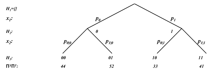
Figure 11.4: The case where players $(X,Y)$ adopt Independent versus Tit-For-Tat strategies in the ${\cal P}^{X}_{B}\times{\cal P}^{Y}_{B}|_{y_{1}=0,y_{2}=x_{1}}$ joint probability space. We write $p_{x_{2}|x_{1}0}=p_{x_{2}|x_{1}}$. Again, neither first nor second stage choices of player $Y$ appear in the game tree as they have been isomorphically constrained and so are not freely varying parameters.

11.4.5 $N=2$ stage: Independent versus Tit-For-Tat strategies

If, on the other hand, players $(X,Y)$ suppose that together they adopt the ${\cal P}^{X}_{B}\times{\cal P}^{Y}_{B}|_{y_{1}=0,y_{2}=x_{1}}$ joint probability space, then the expected payoff function optimization problem becomes

$$X:\max_{p_{1},p_{1|00},p_{1|10}}\;\;\langle\Pi^{X}\rangle = 4+p_{1}+\left[1-p_{1}\right]p_{1|00}+p_{1}\left[p_{1|10}-2\right]$$

$$\langle\Pi^{Y}\rangle = 4-2p_{1}-2\left[1-p_{1}\right]p_{1|00}+p_{1}\left[1-2p_{1|10}\right].$$ (11.29)

As such, the expected payoff functions are dependent only on the freely varying parameters $[p_{1},p_{1|00},p_{1|10}]$ so the relevant gradient operator used by both players in their analysis is

$$\nabla = \left[\frac{\partial}{\partial p_{1}},\frac{\partial}{\partial p_{1|00}},\frac{\partial}{\partial p_{1|10}}\right].$$ (11.30)

Consequently, optimization for player $X$ gives

$$\frac{\partial\langle\Pi^{X}\rangle}{\partial p_{1|00}} = \left[1-p_{1}\right]\geq 0$$

$$\frac{\partial\langle\Pi^{X}\rangle}{\partial p_{1|10}} = p_{1}\geq 0,$$ (11.31)

leading, essentially, to defection on all second stage histories via $p_{1|x_{1}0}=1$ on every pathway. Taking account of these last stage results then gives

$$X:\max_{p_{1}}\;\;\langle\Pi^{X}\rangle = 5-p_{1}$$

$$\frac{\partial\langle\Pi^{X}\rangle}{\partial p_{1}} = -1,$$ (11.32)

so player $X$ cooperates in the first stage with certainty through the choice $p_{1}=0$. Altogether, the ${\cal P}^{X}_{B}\times{\cal P}^{Y}_{B}|_{y_{1}=0,y_{2}=x_{1}}$ joint probability space leads players to the move combinations $(x_{1},y_{1},x_{2},y_{2})=(0,0,1,0)$ to garner payoffs $\left(\langle\Pi^{X}\rangle,\langle\Pi^{Y}\rangle\right)=(5,2)$.

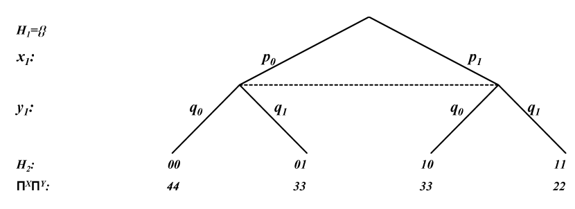
Figure 11.5: The case where players $(X,Y)$ adopt Markovian versus Markovian strategies in the ${\cal P}^{X}_{B}|_{x_{2}=y_{1}}\times{\cal P}^{Y}_{B}|_{y_{2}=x_{1}}$ joint probability space. As both players functionally assign their second stage choices, the only freely varying parameters are the first stage choices of each player.

11.4.6 $N=2$ stage: Markovian versus Markovian strategies

Suppose now that players $(X,Y)$ jointly assume they both adopt the ${\cal P}^{X}_{B}|_{x_{2}=y_{1}}\times{\cal P}^{Y}_{B}|_{y_{2}=x_{1}}$ probability space. After resolution of the adopted isomorphic constraints, the expected payoff function optimization problems become

$$X:\max_{p_{1}}\;\;\langle\Pi^{X}\rangle = 4-p_{1}-q_{1}$$

$$Y:\max_{q_{1}}\;\;\langle\Pi^{Y}\rangle = 4-p_{1}-q_{1},$$ (11.33)

which are dependent only on the freely varying parameters $[p_{1},q_{1}]$, so immediately, the gradient operator used by each player in their analysis is

$$\nabla = \left[\frac{\partial}{\partial p_{1}},\frac{\partial}{\partial q_{1}}\right].$$ (11.34)

Optimization then proceeds straightforwardly giving respectively for each player

$$\frac{\partial\langle\Pi^{X}\rangle}{\partial p_{1}} = -1$$

$$\frac{\partial\langle\Pi^{Y}\rangle}{\partial q_{1}} = -1,$$ (11.35)

ensuring that in this space, both players cooperate with certainty in the first stage by setting $p_{1}=q_{1}=0$. Altogether, when players $(X,Y)$ adopt the ${\cal P}^{X}_{B}|_{x_{2}=y_{1}}\times{\cal P}^{Y}_{B}|_{y_{2}=x_{1}}$ joint probability space, they cooperate via the move combinations $(x_{1},y_{1},x_{2},y_{2})=(0,0,0,0)$ to garner payoffs $\left(\langle\Pi^{X}\rangle,\langle\Pi^{Y}\rangle\right)=(4,4)$. That is, under a joint constraint where each player mimics their opponent’s previous moves, a strategy of cooperation is rational as it maximizes expected payoffs for both players.

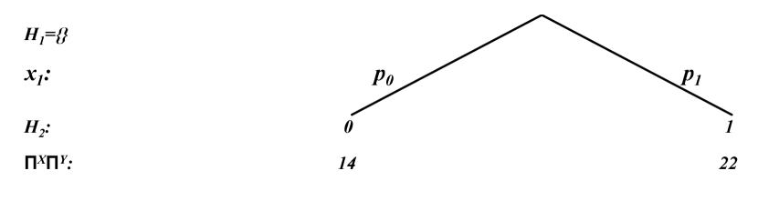
Figure 11.6: The case where players $(X,Y)$ adopt Markovian versus All Defect strategies in the ${\cal P}^{X}_{B}|_{x_{2}=y_{1}}\times{\cal P}^{Y}_{B}|_{y_{1}=y_{2}=1}$ joint probability space. As both players functionally assign all of their second stage choices while player $Y$ defects with certainty in the first stage, the only freely varying parameter left is the first stage choice of player $X$ reducing the game to being a single-player-single-stage situation as shown.

11.4.7 $N=2$ stage: Markovian versus All Defect strategies

Suppose now that players $(X,Y)$ analyze the case where they jointly adopt the ${\cal P}^{X}_{B}|_{x_{2}=y_{1}}\times{\cal P}^{Y}_{B}|_{y_{1}=y_{2}=1}$ probability space. The resolution of the adopted constraints means that the expected payoff function optimization problem for the players becomes

$$X:\max_{p_{1}}\;\;\langle\Pi^{X}\rangle = 1+p_{1}$$

$$\langle\Pi^{Y}\rangle = 4-2p_{1},$$ (11.36)

which are dependent only on the freely varying parameter $p_{1}$, so immediately, the gradient operator used by each player in their analysis is

$$\nabla=\frac{\partial}{\partial p_{1}}.$$ (11.37)

Player $X$ then evaluates

$$\frac{\partial\langle\Pi^{X}\rangle}{\partial p_{1}}=1,$$ (11.38)

ensuring that this player defects with certainty in the first stage by setting $p_{1}=1$. Altogether, when players $(X,Y)$ jointly adopt the ${\cal P}^{X}_{B}|_{x_{2}=y_{1}}\times{\cal P}^{Y}_{B}|_{y_{1}=y_{2}=1}$ probability space, they generate the optimal move combination $(x_{1},y_{1},x_{2},y_{2})=(1,1,1,1)$ to garner payoffs $\left(\langle\Pi^{X}\rangle,\langle\Pi^{Y}\rangle\right)=(2,2)$.

Figure 11.7: The case where players $(X,Y)$ adopt Markovian verses Tit-For-Tat strategies in the ${\cal P}^{X}_{B}|_{x_{2}=y_{1}}\times{\cal P}^{Y}_{B}|_{y_{1}=0,y_{2}=x_{1}}$ joint probability space. As both players functionally assign all of their second stage choices while player $Y$ cooperates with certainty in the first stage, the only freely varying parameter left is the first stage choice of player $X$ reducing the game to being a single-player-single-stage situation as shown.

11.4.8 $N=2$ stage: Markovian verses Tit-For-Tat strategies

Suppose now that players $(X,Y)$ jointly assume that together they adopt the ${\cal P}^{X}_{B}|_{x_{2}=y_{1}}\times{\cal P}^{Y}_{B}|_{y_{1}=0,y_{2}=x_{1}}$ probability space. After resolution of the isomorphic constraints, the expected payoff function optimization problems become

$$X:\max_{p_{1}}\;\;\langle\Pi^{X}\rangle = 4-p_{1}$$

$$\langle\Pi^{Y}\rangle = 4-p_{1},$$ (11.39)

which are dependent only on the freely varying parameter $p_{1}$, so immediately, the gradient operator used by each player in their analysis is

$$\nabla=\frac{\partial}{\partial p_{1}}.$$ (11.40)

Player $X$ then evaluates

$$\frac{\partial\langle\Pi^{X}\rangle}{\partial p_{1}}=-1,$$ (11.41)

ensuring that this player cooperates with certainty in the first stage by setting $p_{1}=0$. Altogether, when players $(X,Y)$ jointly adopt the ${\cal P}^{X}_{B}|_{x_{2}=y_{1}}\times{\cal P}^{Y}_{B}|_{y_{1}=0,y_{2}=x_{1}}$ probability space, they generate the optimal move combination $(x_{1},y_{1},x_{2},y_{2})=(0,0,0,0)$ to garner payoffs $\left(\langle\Pi^{X}\rangle,\langle\Pi^{Y}\rangle\right)=(4,4)$.

11.4.9 $N=2$ stage: Comparing payoffs

The remainder of the possible probability spaces that the players might analyze, Tit-For-Tat versus Tit-For-Tat (${\cal P}^{X}_{B}|_{x_{1}=0,x_{2}=y_{1}}\times{\cal P}^{Y}_{B}|_{y_{1}=0,y_{2}=x_{1}}$), Tit-For-Tat versus All Defect (${\cal P}^{X}_{B}|_{x_{1}=0,x_{2}=y_{1}}\times{\cal P}^{Y}_{B}|_{y_{1}=y_{2}=1}$), and All Defect versus All defect (${\cal P}^{X}_{B}|_{x_{1}=x_{2}=1}\times{\cal P}^{Y}_{B}|_{y_{1}=y_{2}=1}$), possess no free variables whatsoever and so merely involve an evaluation of the expected payoffs in each case. Altogether, under the assumption that either player might adopt any of the four probability spaces considered here, then players must compare 16 possible isomorphically constrained optima to locate their optimal choice of probability space. The comparison table showing every possible combination of adopted probability space for either player is

$$\begin{array}[]{c|cccc}\left(\langle\Pi^{X}\rangle,\langle\Pi^{Y}\rangle\right)&{\cal P}^{Y}_{B}|_{y_{2}=x_{1}}&{\cal P}^{Y}_{B}&{\cal P}^{Y}_{B}|_{y_{1}=0,y_{2}=x_{1}}&{\cal P}^{Y}_{B}|_{y_{1}=y_{2}=1}\\ \hline\cr&&&&\\ {\cal P}^{X}_{B}|_{x_{2}=y_{1}}&(4,4)&(3,3)&(4,4)&(2,2)\\ &&&&\\ {\cal P}^{X}_{B}&(3,3)&(2,2)&(5,2)&(2,2)\\ &&&&\\ {\cal P}^{X}_{B}|_{x_{1}=0,x_{2}=y_{1}}&(4,4)&(2,5)&(4,4)&(1,4)\\ &&&&\\ {\cal P}^{X}_{x_{1}=x_{2}=1}&(2,2)&(2,2)&(4,1)&(2,2).\\ &&&&\\ \end{array}$$ (11.42)

This table of alternate expected payoffs makes it evident that the Tit-For-Tat and All Defect probability spaces are weakly dominated by the Markovian and Independent probability spaces. Player’s choices of optimal probability spaces then come down effectively to a comparison of the Markovian or the Independent probability spaces. Perusal of the table shows that adopting the Markovian probability space offers the better returns to either player.

Given this admittedly small set of possible strategy constraints, rational players will maximize their expected payoffs by adopting a Markovian strategy and rationally cooperate in the finite iterated prisoner’s dilemma. The traditional result of conventional game analysis that mutual all defection is the unique Nash equilibria for this game is an incomplete analysis based on the unjustified restriction that players can only employ a restricted set of independent probability distributions.

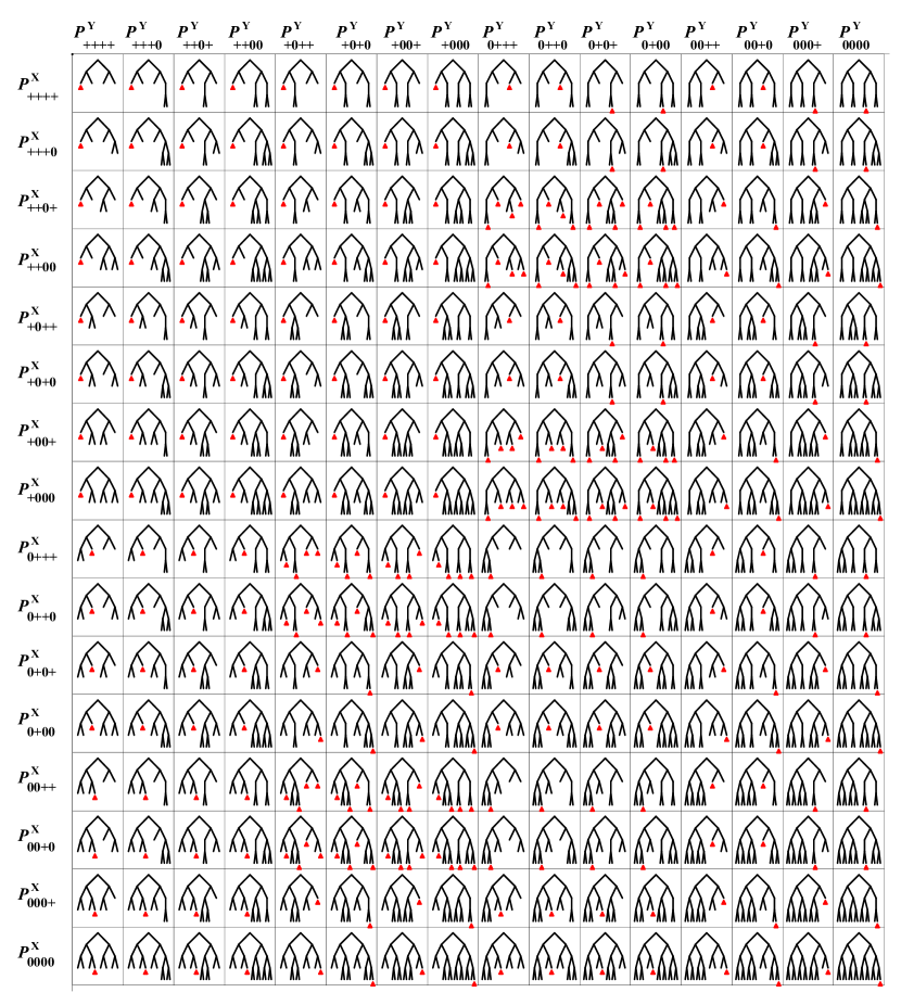
Figure 11.8: The generated trees and the equilibrium pathways (indicated by small dots, with multiple dots indicating mixed equilibrium pathways) assuming that player $X$ adopts the probability space shown on the vertical axis and that player $Y$ adopts the probability space shown horizontally. (When the $x_{2}$ choice is correlated and the $y_{2}$ choice is independent, a vertical line is shown to maintain the relative spacings of each tree.) The expected payoffs under each strategy combination are shown in Table 11.1.

11.4.10 $N=2$ stage: Extended isomorphic constraints

An immediate question of interest is whether the conclusion that cooperation is rational survives an extended analysis employing a wider class of possible isomorphic constraints which we investigate now. We here examine a total of 256 alternate probability spaces for the $N=2$ stage iterated prisoner’s dilemma game. The resulting game trees are shown in Fig. 11.8 (appearing in exploded form), with optimized expected payoffs derived in each joint probability space shown in Table 11.1.

We suppose that each of our players, denoted $Z\in\{X,Y\}$, chooses whether each of their four second stage behavioural strategies $P^{Z}(z_{2}|x_{1}y_{1})$ are either independent, denoted “$0$”, or perfectly correlated to their opponent’s previous move, denoted “$+$”. (Perfect anti-correlations are also possible, but these are not considered here.) There are four histories $(x_{1},y_{1})\in\{(0,0),(0,1),(1,0),(1,1)\}$. Admittedly, it is unusual to specify whether a behavioural strategy implemented at a single node of a game tree is either independent of previous events or correlated with previous events. However, there is nothing preventing this from occurring—it might not be an optimal choice but it is a possible set of choices that a player might make when optimizing their payoffs over a game tree.

Consequently, if player $Z$ chooses to make all of the second stage behavioural strategy probability distributions $P^{Z}(z_{2}|x_{1}y_{1})$ independent then the adopted space is ${\cal P}^{Z}_{0000}$. This means that the randomized choices player $Z$ makes at every second stage node of the game tree are independent of every other event (as is usually the case). However, if $Z$ chooses to functionally correlate all of their second stage behavioural strategy probability distributions $P^{Z}(z_{2}|x_{1}y_{1})$ then the adopted space is ${\cal P}^{Z}_{++++}$. In this case, the dice roll that $Z$ uses to make their choice of $y_{2}$ in the case $(x_{1},y_{1})=(0,0)$ will be perfectly correlated to the previous event $x_{1}=0$. As noted, this is an unusual choice but nevertheless it is still a possible choice. Intermediate cases include when, for instance, $Z$ decides to make $P^{Z}(z_{2}|00)$ and $P^{Z}(z_{2}|10)$ independent, and to functionally correlate $P^{Z}(z_{2}|01)$ and $P^{Z}(z_{2}|11)$, in which case the adopted space is ${\cal P}^{Z}_{0+0+}$, and so on. Altogether, there are 16 possible choices that player $Z$ might make about their probability space, namely $\{{\cal P}^{Z}_{0000},{\cal P}^{Z}_{000+},{\cal P}^{Z}_{00+0},{\cal P}^{Z}_{00++},\dots,{\cal P}^{Z}_{++++}\}$. In combination, both players can jointly adopt one of $16^{2}=256$ different joint probability spaces, in each of which a potentially different constrained equilibria exists, and all of these optima must be compared so that players can decide which probability space they can rationally choose.

$\left(\langle\Pi^{X}\rangle,\langle\Pi^{Y}\rangle\right)$
	${\cal P}^{Y}_{++++}$	${\cal P}^{Y}_{+++0}$	${\cal P}^{Y}_{++0+}$	${\cal P}^{Y}_{++00}$	${\cal P}^{Y}_{+0++}$	${\cal P}^{Y}_{+0+0}$	${\cal P}^{Y}_{+00+}$	${\cal P}^{Y}_{+000}$	${\cal P}^{Y}_{0+++}$	${\cal P}^{Y}_{0++0}$	${\cal P}^{Y}_{0+0+}$	${\cal P}^{Y}_{0+00}$	${\cal P}^{Y}_{00++}$	${\cal P}^{Y}_{00+0}$	${\cal P}^{Y}_{000+}$	${\cal P}^{Y}_{0000}$
${\cal P}^{X}_{++++}$	(4,4)	(4,4)	(4,4)	(4,4)	(4,4)	(4,4)	(4,4)	(4,4)	(3,3)	(3,3)	(3,3)	(3,3)	(3,3)	(3,3)	(3,3)	(3,3)
${\cal P}^{X}_{+++0}$	(4,4)	(4,4)	(4,4)	(4,4)	(4,4)	(4,4)	(4,4)	(4,4)	(3,3)	(3,3)	(3,3)	(3,3)	(3,3)	(3,3)	(3,3)	(3,3)
${\cal P}^{X}_{++0+}$	(4,4)	(4,4)	(4,4)	(4,4)	(4,4)	(4,4)	(4,4)	(4,4)	($\frac{8}{3},\frac{7}{3}$)	($\frac{8}{3},\frac{7}{3}$)	($\frac{8}{3},\frac{7}{3}$)	($\frac{8}{3},\frac{7}{3}$)	(2,2)	(2,2)	(2,2)	(2,2)
${\cal P}^{X}_{++00}$	(4,4)	(4,4)	(4,4)	(4,4)	(4,4)	(4,4)	(4,4)	(4,4)	($\frac{8}{3},\frac{7}{3}$)	($\frac{8}{3},\frac{7}{3}$)	($\frac{8}{3},\frac{7}{3}$)	($\frac{8}{3},\frac{7}{3}$)	(2,2)	(2,2)	(2,2)	(2,2)
${\cal P}^{X}_{+0++}$	(4,4)	(4,4)	(4,4)	(4,4)	(4,4)	(4,4)	(4,4)	(4,4)	(3,3)	(3,3)	(3,3)	(3,3)	(3,3)	(3,3)	(3,3)	(3,3)
${\cal P}^{X}_{+0+0}$	(4,4)	(4,4)	(4,4)	(4,4)	(4,4)	(4,4)	(4,4)	(4,4)	(3,3)	(3,3)	(3,3)	(3,3)	(3,3)	(3,3)	(3,3)	(3,3)
${\cal P}^{X}_{+00+}$	(4,4)	(4,4)	(4,4)	(4,4)	(4,4)	(4,4)	(4,4)	(4,4)	($\frac{8}{3},\frac{7}{3}$)	($\frac{8}{3},\frac{7}{3}$)	($\frac{8}{3},\frac{7}{3}$)	($\frac{8}{3},\frac{7}{3}$)	(2,2)	(2,2)	(2,2)	(2,2)
${\cal P}^{X}_{+000}$	(4,4)	(4,4)	(4,4)	(4,4)	(4,4)	(4,4)	(4,4)	(4,4)	($\frac{8}{3},\frac{7}{3}$)	($\frac{8}{3},\frac{7}{3}$)	($\frac{8}{3},\frac{7}{3}$)	($\frac{8}{3},\frac{7}{3}$)	(2,2)	(2,2)	(2,2)	(2,2)
${\cal P}^{X}_{0+++}$	(3,3)	(3,3)	(3,3)	(3,3)	($\frac{7}{3},\frac{8}{3}$)	($\frac{7}{3},\frac{8}{3}$)	($\frac{7}{3},\frac{8}{3}$)	($\frac{7}{3},\frac{8}{3}$)	(3,3)	(3,3)	(3,3)	(3,3)	(3,3)	(3,3)	(3,3)	(3,3)
${\cal P}^{X}_{0++0}$	(3,3)	(3,3)	(3,3)	(3,3)	($\frac{7}{3},\frac{8}{3}$)	($\frac{7}{3},\frac{8}{3}$)	($\frac{7}{3},\frac{8}{3}$)	($\frac{7}{3},\frac{8}{3}$)	(3,3)	(3,3)	(3,3)	(3,3)	(3,3)	(3,3)	(3,3)	(3,3)
${\cal P}^{X}_{0+0+}$	(3,3)	(3,3)	(3,3)	(3,3)	(2,2)	(2,2)	(2,2)	(2,2)	(3,3)	(3,3)	(3,3)	(3,3)	(2,2)	(2,2)	(2,2)	(2,2)
${\cal P}^{X}_{0+00}$	(3,3)	(3,3)	(3,3)	(3,3)	(2,2)	(2,2)	(2,2)	(2,2)	(3,3)	(3,3)	(3,3)	(3,3)	(2,2)	(2,2)	(2,2)	(2,2)
${\cal P}^{X}_{00++}$	(3,3)	(3,3)	(3,3)	(3,3)	($\frac{7}{3},\frac{8}{3}$)	($\frac{7}{3},\frac{8}{3}$)	($\frac{7}{3},\frac{8}{3}$)	($\frac{7}{3},\frac{8}{3}$)	(3,3)	(3,3)	(3,3)	(3,3)	(3,3)	(3,3)	(3,3)	(3,3)
${\cal P}^{X}_{00+0}$	(3,3)	(3,3)	(3,3)	(3,3)	($\frac{7}{3},\frac{8}{3}$)	($\frac{7}{3},\frac{8}{3}$)	($\frac{7}{3},\frac{8}{3}$)	($\frac{7}{3},\frac{8}{3}$)	(3,3)	(3,3)	(3,3)	(3,3)	(3,3)	(3,3)	(3,3)	(3,3)
${\cal P}^{X}_{000+}$	(3,3)	(3,3)	(3,3)	(3,3)	(2,2)	(2,2)	(2,2)	(2,2)	(3,3)	(3,3)	(3,3)	(3,3)	(2,2)	(2,2)	(2,2)	(2,2)
${\cal P}^{X}_{0000}$	(3,3)	(3,3)	(3,3)	(3,3)	(2,2)	(2,2)	(2,2)	(2,2)	(3,3)	(3,3)	(3,3)	(3,3)	(2,2)	(2,2)	(2,2)	(2,2)

Table 11.1: Table of expected payoffs for various isomorphically constrained equilibria. The trees generated under each joint probability space and their equilibrium pathways are shown in Fig. 11.8.

Here, without presenting the details of the calculations, we show the results of comparing all 16 possible probability spaces of each player against all 16 of their opponent’s possible probability spaces—see Fig. 11.8 and Table 11.1. (In cases where players are indifferent to move choice, we arbitrarily choose cooperation.) We also note that it turns out that there is only one isomorphically constrained equilibria in each probability space and some of these are in mixed strategies.

It is of course possible to use Table 11.1 to locate globally optimal choices of probability space. Examination of this table shows that many rows and columns are identical. Numbering each row from top to bottom by $r_{i}$ and each column from left to right by $c_{j}$ ($1\leq i,j\leq 16$), we have $r_{1}=r_{2}=r_{5}=r_{6}$, $r_{3}=r_{4}=r_{7}=r_{8}$, $r_{9}=r_{10}=r_{13}=r_{14}$, and $r_{11}=r_{12}=r_{15}=r_{16}$. As well, we have $c_{1}=c_{2}=c_{3}=c_{4}$, $c_{5}=c_{6}=c_{7}=c_{8}$, $c_{9}=c_{10}=c_{11}=c_{12}$, and $c_{13}=c_{14}=c_{15}=c_{16}$. Removing all identical rows and columns leaves the variational payoff table

$$\begin{array}[]{c|cccc}\left(\langle\Pi^{X}\rangle,\langle\Pi^{Y}\rangle\right)&{\cal P}^{Y}_{++++}&{\cal P}^{Y}_{+000}&{\cal P}^{Y}_{0+++}&{\cal P}^{Y}_{0000}\\ \hline\cr&&&&\\ {\cal P}^{X}_{++++}&(4,4)&(4,4)&(3,3)&(3,3)\\ &&&&\\ {\cal P}^{X}_{+000}&(4,4)&(4,4)&(\frac{8}{3},\frac{7}{3})&(2,2)\\ &&&&\\ {\cal P}^{X}_{0+++}&(3,3)&(\frac{7}{3},\frac{8}{3})&(3,3)&(3,3)\\ &&&&\\ {\cal P}^{X}_{0000}&(3,3)&(2,2)&(3,3)&(2,2)\\ &&&&\\ \end{array}.$$ (11.43)

An inspection by eye (checked by numerical calculation) confirms that the only “equilibria” in this reduced table of constrained equilibria are the uninteresting combinations in the bottom right of $\left({\cal P}^{X}_{0000},{\cal P}^{Y}_{0+++}\right)$, $\left({\cal P}^{X}_{0+++},{\cal P}^{Y}_{0000}\right)$, and $\left({\cal P}^{X}_{0+++},{\cal P}^{Y}_{0+++}\right)$, and the more interesting payoff maximizing equilibria in the top left of $\left({\cal P}^{X}_{++++},{\cal P}^{Y}_{++++}\right)$, $\left({\cal P}^{X}_{++++},{\cal P}^{Y}_{+000}\right)$, $\left({\cal P}^{X}_{+000},{\cal P}^{Y}_{++++}\right)$, and $\left({\cal P}^{X}_{+000},{\cal P}^{Y}_{+000}\right)$. In these latter equilibria, as long as players functionally correlate their behavioural strategies in the second stage following from the history $(x_{1},y_{1})=(0,0)$, then they will conclude that it is payoff maximizing to cooperate in this finite iterated prisoner’s dilemma to garner joint payoffs of $\left(\langle\Pi^{X}\rangle,\langle\Pi^{Y}\rangle\right)=(4,4)$. Any other choice is not rational.

Again, we conclude that players of unrestricted rationality will cooperate in the finite iterated prisoner’s dilemma. As such, our analysis reconciles game theoretic predictions and the cooperative human behaviours observed in experimental tests [96, 97].

11.5 $N>2$ stages: A limited investigation

We now consider the case where the number of stages is known and finite and greater than two. We will consider how players might vary their choice of probability space or of isomorphic constraints so as to optimize the expected payoffs of Eq. 11.2 when the number of stages $N>2$. Our analysis will be limited as with each additional stage the number of possible joint probability spaces that might be considered by the players increases exponentially. In the present section, we suppose that players adopt either a conventional independent behavioural space or a Markovian space in which current stage choices are correlated to the immediately preceding stage choices. In more detail, the choices open to the players include adopting either a conventional independent behavioural strategy space ${\cal P}^{X}_{B}$ and ${\cal P}^{Y}_{B}$, or a Markovian probability space ${\cal P}^{X}_{B}|_{x_{n}=y_{n-1}}$ and ${\cal P}^{Y}_{B}|_{y_{n}=x_{n-1}}$. In subsequent sections, we will examine the various combinations of probability space that might be adopted, and we will finally allow players to try preemptive defection near the terminal stages of the game. This will allow us to check whether these defections propagate backwards as required by a standard backwards induction analysis.

11.5.1 $N\geq 2$: Independent strategies

We first presume that players $X$ and $Y$ each examine the case where they jointly adopt the space ${\cal P}^{X}_{B}\times{\cal P}^{Y}_{B}$ in which all of their behavioural strategies on every possible history set are independent of any other event. The players seek to optimize their respective expected payoff functions in Eq. 11.2.

Every behavioural probability parameter (after normalization) is independent so the gradient operator used by both players to analyze optimal play are

$$\nabla=\left[\frac{d}{dP^{X}(1)},\frac{d}{dP^{Y}(1)},\frac{d}{dP^{X}(1|H_{1})},\frac{d}{dP^{Y}(1|H_{1})},\dots,\frac{d}{dP^{X}(1|H_{N})},\frac{d}{dP^{Y}(1|H_{N})}\right].$$ (11.44)

where gradients are taken with respect to all possible history sets $H_{n}$. Also, gradients are taken via total derivatives rather than partial derivatives to facilitate calculations—the normalization constraint $P^{X}(0|H_{n})=1-P^{X}(1|H_{n})$ allows writing the total rate of change of the expected payoff function with respect to the changing probability parameters as

$$\frac{d\langle\Pi^{X}\rangle}{dP^{X}(1|H_{n})}=\frac{\partial\langle\Pi^{X}\rangle}{\partial P^{X}(1|H_{n})}-\frac{\partial\langle\Pi^{X}\rangle}{\partial P^{X}(0|H_{n})}.$$ (11.45)

Each player can then straightforwardly use this gradient operator defined within the joint probability space ${\cal P}^{X}_{B}\times{\cal P}^{Y}_{B}$ to evaluate their optimal choices. In particular, the shorthand notation $H_{n}=\{H_{n-1},x_{n},y_{n}\}$ and some algebra allows writing the optimization conditions for player $X$ as the set of simultaneous equations

$$\frac{d\langle\Pi^{X}\rangle}{dP^{X}(1)} = \dots$$

$$\vdots$$

$$\frac{d\langle\Pi^{X}\rangle}{dP^{X}(1|H_{n-1})} = 1+$$

$$\sum_{\stackrel{{\scriptstyle x_{1}\dots x_{N-2}=0}}{{y_{1}\dots y_{N-2}=0}}}^{1}P^{X}(x_{1})P^{Y}(y_{1})\dots P^{X}(x_{N-2}|H_{N-2})P^{Y}(y_{N-2}|H_{N-2})\times$$

$$\sum_{y_{N-1}=0}^{1}P^{Y}(y_{N-1}|H_{N-1})\sum_{x_{N}y_{N}=0}^{1}(x_{N}-2y_{N})\times$$

$$\hskip 28.45274pt\left[\right.P^{X}(x_{N}|H_{N-1},1,y_{N-1})P^{Y}(y_{N}|H_{N-1},1,y_{N-1})-$$

$$\hskip 56.9055ptP^{X}(x_{N}|H_{N-1},0,y_{N-1})P^{Y}(y_{N}|H_{N-1},0,y_{N-1})\left.\right]$$

$$\frac{d\langle\Pi^{X}\rangle}{dP^{X}(1|H_{N})} = 1.$$ (11.46)

The equivalent simultaneous optimization conditions for player $P_{y}$ are

$$\frac{d\langle\Pi^{Y}\rangle}{dP^{Y}(1)} = \dots$$

$$\vdots$$

$$\frac{d\langle\Pi^{Y}\rangle}{dP^{Y}(1|H_{N-1})} = 1+$$

$$\sum_{\stackrel{{\scriptstyle x_{1}\dots x_{N-2}=0}}{{y_{1}\dots y_{N-2}=0}}}^{1}P^{X}(x_{1})P^{Y}(y_{1})\dots P^{X}(x_{N-2}|H_{N-2})P^{Y}(y_{N-2}|H_{N-2})\times$$

$$\sum_{x_{N-1}=0}^{1}P^{X}(x_{N-1}|H_{N-1})\sum_{x_{N}y_{N}=0}^{1}(y_{N}-2x_{N})\times$$

$$\hskip 28.45274pt\left[\right.P^{X}(x_{N}|H_{N-1},x_{N-1},1)P^{Y}(y_{N}|H_{N-1},x_{N-1},1)-$$

$$\hskip 56.9055ptP^{X}(x_{N}|H_{N-1},x_{N-1},0)P^{Y}(y_{N}|H_{N-1},x_{N-1},0)\left.\right]$$

$$\frac{d\langle\Pi^{Y}\rangle}{dP^{Y}(1|H_{N})} = 1.$$ (11.47)

Subsequently each player solves their respective sets of simultaneous equations to maximize their expected payoff in the joint probability space ${\cal P}^{X}_{B}\times{\cal P}^{Y}_{B}$ by setting $P^{X}(1|H_{N})=1$ and $P^{Y}(1|H_{N})=1$ for all history sets $H_{N}$, and by setting $P^{X}(1|H_{N-1})=1$ and $P^{Y}(1|H_{N-1})=1$ for all history sets $H_{N-1}$, and so on. The final result is that both players defect at every stage giving optimal choices as $(x_{n},y_{n})=(1,1)\equiv(D,D)$ for all $n$. At this point, payoffs are $(\langle\Pi^{X}_{B}\rangle,\langle\Pi^{Y}_{B}\rangle)=(N,N)$.

11.5.2 $N\geq 2$: Markovian versus Independent spaces

Suppose now that players $X$ and $Y$ jointly examine the case where $Y$ adopts the independent probability space while $X$ adopts isomorphic constraints to implement Markovian play. In this case the joint probability space is ${\cal P}^{X}_{B}|_{x_{n}=y_{n-1}}\times{\cal P}^{Y}_{B}$. Here, $X$ adopts the isomorphic constraints

$$x_{n} = y_{n-1}$$

$$P^{X}(x_{n}|H_{n}) = \delta_{x_{n}y_{n-1}},$$ (11.48)

for $2\leq n\leq N$ and on every history $H_{n}$. As usual, these isomorphic constraints must be resolved before the optimization can proceed rendering the optimization problem for each player as

$$X:\max_{P^{X}(1)}\;\;\langle\Pi^{X}\rangle = 2N+\left[\sum_{x_{1}=0}^{1}P^{X}(x_{1})x_{1}\right]+$$

$$-\sum_{n=1}^{N-1}\sum_{x_{1}y_{1}\dots y_{n}=0}^{1}P^{X}(x_{1})P^{Y}(y_{1})\dots P^{Y}(y_{n}|H^{\prime}_{n})y_{n}+$$

$$-2\sum_{x_{1}y_{1}\dots y_{N}=0}^{1}P^{X}(x_{1})P^{Y}(y_{1})\dots P^{Y}(y_{N}|H^{\prime}_{N})y_{N},$$

$$Y:\max_{P^{Y}(1),P^{Y}(1|H_{n})}\;\;\langle\Pi^{Y}\rangle = 2N-2\left[\sum_{x_{1}=0}^{1}P^{X}(x_{1})x_{1}\right]+$$

$$-\sum_{n=1}^{N-1}\sum_{x_{1}y_{1}\dots y_{n}=0}^{1}P^{X}(x_{1})P^{Y}(y_{1})\dots P^{Y}(y_{n}|H^{\prime}_{n})y_{n}$$

$$+\sum_{x_{1}y_{1}\dots y_{N}=0}^{1}P^{X}(x_{1})P^{Y}(y_{1})\dots P^{Y}(y_{N}|H^{\prime}_{N})y_{N}.$$

Here, a modified history set appears due to the delta-function constraints so that, for instance, $H^{\prime}_{3}=\{x_{1},y_{1},x_{2},y_{2}\}=\{x_{1},y_{1},y_{1},y_{2}\}$. Hereinafter, primes are dropped.

The shorthand notation $H_{n}=\{H_{n-1},y_{n}\}$ for $n\geq 2$ and some algebra allows writing the optimization conditions for player $Y$ as the set of simultaneous equations

$$\frac{d\langle\Pi^{Y}\rangle}{dP^{Y}(1)} = \dots,$$

$$\vdots$$

$$\frac{d\langle\Pi^{Y}\rangle}{dP^{Y}(1|H_{N-1})} = -1+$$

$$+\sum_{x_{1}y_{1}\dots y_{N-2}=0}^{1}P^{X}(x_{1})P^{Y}(y_{1})\dots P^{Y}(y_{N-2}|H_{N-2})\times$$

$$\sum_{y_{N}=0}^{1}y_{N}\left[P^{Y}(y_{N}|H_{N-1},1)-P^{Y}(y_{N}|H_{N-1},0)\right],$$

$$\frac{d\langle\Pi^{Y}\rangle}{dP(1|H_{N})} = 1.$$ (11.50)

Hence, player $Y$ optimizes their payoff by setting $P^{Y}(1|H_{N})=1$ for every history set $H_{N}$, and by setting $P^{Y}(1|H_{N-1})=0$ for every history set $H_{N-1}$, and eventually by setting $P^{Y}(1|H_{n})=0$ for $1\leq n\leq(N-1)$. That is, $Y$ maximizes their expected payoff by cooperating in every stage but the last.

Player $X$ is well able to calculate the same optimal choices for their opponent, and uses this knowledge to simplify their own optimization problem to eventually give the condition

$$\frac{d\langle\Pi^{X}\rangle}{dP^{X}(1)}=1.$$ (11.51)

Consequently, $X$ optimizes their expected payoff by setting $P^{X}(1)=1$ and so defects in this first stage.

In the joint probability space ${\cal P}^{X}_{B}|_{x_{n}=y_{n-1}}\times{\cal P}^{Y}_{B}$, the players locate the constrained equilibria at the point $(x_{1},y_{1},\ldots,y_{N})=(1,0,\dots,0,1)$ generating the play sequence

$$(x_{n},y_{n}) = (1,0),(0,0),\dots,(0,0),(0,1)$$ (11.52)

$$= (D,C)(C,C)\dots(C,C)(C,D),$$

to give expected payoffs $(\langle\Pi^{X}\rangle,\langle\Pi^{Y}\rangle)=(2N-1,2N-1)$. Here, $X$ defects in the first stage as their opponent cannot respond without decreasing their payoff, while $Y$ can defect in the last stage when $X$ can no longer respond.

11.5.3 $N\geq 2$: Markovian versus Markovian strategies

Each player might well then analyze the case where both players adopt Markovian strategies and thereby implement the joint probability space ${\cal P}^{X}_{B}|_{x_{n}=y_{n-1}}\times{\cal P}^{Y}_{B}|_{y_{n}=x_{n-1}}$. Here, $X$ adopts the isomorphic constraints

$$x_{n} = y_{n-1}$$

$$P^{X}(x_{n}|H_{n}) = \delta_{x_{n}y_{n-1}},$$ (11.53)

for $2\leq n\leq N$ and every history set $H_{n}$, while $Y$ adopts the isomorphic constraints

$$y_{n} = x_{n-1}$$

$$P^{Y}(y_{n}|H_{n}) = \delta_{y_{n}x_{n-1}},$$ (11.54)

for $2\leq n\leq N$ and every history set $H_{n}$. These constraints must be resolved before the optimization can proceed reducing the optimization problem for each player to

$$X:\max_{P^{X}(1)}\;\;\langle\Pi^{X}\rangle = \sum_{x_{1},y_{1}=0}^{1}P^{X}(x_{1})P^{Y}(y_{1})\Pi^{X}(x_{1},y_{1}),$$

$$Y:\max_{P^{Y}(1)}\;\;\langle\Pi^{Y}\rangle = \sum_{x_{1},y_{1}=0}^{1}P^{X}(x_{1})P^{Y}(y_{1})\Pi^{Y}(x_{1},y_{1}),$$ (11.55)

where the payoffs for a given play sequence $(x_{1},y_{1})$ are

$$\Pi^{X}(x_{1},y_{1}) = \left\{\begin{array}[]{ll}2N-\frac{N}{2}x_{1}-\frac{N}{2}y_{1},&N\mbox{ even},\\ &\\ 2N-\frac{N-3}{2}x_{1}-\frac{N+3}{2}y_{1},&N\mbox{ odd},\\ \end{array}\right.$$ (11.59)

$$\Pi^{Y}(x_{1},y_{1}) = \left\{\begin{array}[]{lc}2N-\frac{N}{2}x_{1}-\frac{N}{2}y_{1},&N\mbox{ even},\\ &\\ 2N-\frac{N+3}{2}x_{1}-\frac{N-3}{2}y_{1},&N\mbox{ odd}.\\ \end{array}\right.$$ (11.63)

The adoption of the joint probability space ${\cal P}^{X}_{B}|_{x_{n}=y_{n-1}}\times{\cal P}^{Y}_{B}|_{y_{n}=x_{n-1}}$ has effectively reduced the $N$ stage supergame to a single stage game with variables $x_{1}$ and $y_{1}$ and payoff matrices, for $N$ even of

$$\begin{array}[]{cc}&Y\\ X&\begin{array}[]{c|cc}(\Pi^{X},\Pi^{Y})&C&D\\ \hline\cr C&(2N,2N)&(\frac{3}{2}N,\frac{3}{2}N)\\ D&(\frac{3}{2}N,\frac{3}{2}N)&(N,N),\\ \end{array}\end{array}$$ (11.64)

and for odd $N$ of

$$\begin{array}[]{cc}&Y\\ X&\begin{array}[]{c|cc}(\Pi^{X},\Pi^{Y})&C&D\\ \hline\cr C&(2N,2N)&\frac{3}{2}[N-1,N+1]\\ D&\frac{3}{2}[N+1,N-1]&(N,N).\\ \end{array}\end{array}$$ (11.65)

That is, in the joint probability space ${\cal P}^{X}_{B}|_{x_{n}=y_{n-1}}\times{\cal P}^{Y}_{B}|_{y_{n}=x_{n-1}}$, the normal form game (and equivalent game tree) is described by an effective payoff matrix with altered off-diagonal elements which naturally modify equilibria.

As usual, the constrained equilibria in the joint space ${\cal P}^{X}_{B}|_{x_{n}=y_{n-1}}\times{\cal P}^{Y}_{B}|_{y_{n}=x_{n-1}}$ are now located via

$$\frac{d\langle\Pi^{X}\rangle}{dP^{X}(1)} = \left\{\begin{array}[]{ll}-\frac{N}{2},&N\mbox{ even},\\ &\\ -\frac{1}{2}(N-3),&N\mbox{ odd},\\ \end{array}\right.$$ (11.69)

$$\frac{d\langle\Pi^{Y}\rangle}{dP^{Y}(1)} = \left\{\begin{array}[]{lc}-\frac{N}{2},&N\mbox{ even},\\ &\\ -\frac{1}{2}(N-3),&N\mbox{ odd}.\\ \end{array}\right.$$ (11.73)

Thus, for either $N$ even or for $N$ odd and greater than 3 we have the equilibrium points $P^{X}(1)=0$ and $P^{Y}(1)=0$ or $(x_{1},y_{1})=(0,0)\equiv(C,C)$. Alternatively, for $N=1$ the equilibria is $P^{X}(1)=1$ and $P^{Y}(1)=1$ or $(x_{1},y_{1})=(1,1)\equiv(D,D)$. When $N=3$ these conditions are satisfied for any values of $(x_{1},y_{1})$ requiring examination of actual payoffs motivating the selection $(x_{1},y_{1})=(0,0)\equiv(C,C)$. The generated sequences of play are

$$\begin{array}[]{c|c|l|c}N&(x_{1},y_{1})&&(\langle\Pi^{X}\rangle,\langle\Pi^{Y}\rangle)\\ \hline\cr&&&\\ 1&(1,1)&(DD)&(1,1)\\ &&&\\ N\geq 2&(0,0)&(CC)\dots(CC)&(2N,2N).\\ \end{array}$$ (11.74)

11.5.4 $N\geq 2$: Comparing payoffs

Each player must then compare the payoffs they expect given that together they jointly adopt the probability space combinations examined above. A table of all possible outcomes for an $N\geq 2$ stage game given the probability spaces under consideration takes the form

$$\begin{array}[]{c|cccc}\left(\langle\Pi^{X}\rangle,\langle\Pi^{Y}\rangle\right)&{\cal P}^{Y}_{B}|_{y_{n}=x_{n-1}}&{\cal P}^{Y}_{B}\\ \hline\cr&&\\ {\cal P}^{X}_{B}|_{x_{n}=y_{n-1}}&(2N,2N)&(2N-1,2N-1)\\ &&\\ {\cal P}^{X}_{B}&(2N-1,2N-1)&(N,N)\\ \end{array}.$$ (11.75)

This table makes it clear that in all the games considered here with two or more stages, players of unbounded rationality maximize their payoffs by each adopting the joint probability space ${\cal P}^{X}_{B}|_{x_{n}=y_{n-1}}\times{\cal P}^{Y}_{B}|_{y_{n}=x_{n-1}}$ in which they adopt isomorphic constraints to correlate all of their choices in every stage after the first with their opponents. Once each player has adopted this particular probability space, this means that they have adopted a “roulette” randomization device which allows them no further choices in any stage after the first, and they have done this as it maximizes their expected payoff.

As in the $N=2$ stage game, we conclude that while players of bounded rationality implementing a conventional analysis will defect in the multiple stage game, players of unrestricted rationality will cooperate in the finite iterated prisoner’s dilemma. Again, our analysis is consistent with observed human behaviours [96, 97].

11.5.5 $N\geq 2$: Endgame analysis

The simplified analysis of the previous section does not allow consideration of “endgame” strategies where players seek to defect in the final stages of a multiple stage game to preempt the defection of their opponent. It is these preemptive defections in backwards induction which conventionally require players of bounded rationality to defect in every stage of the finite iterated prisoner’s dilemma. The question now is, does such mutual preemption apply in an unbounded rational analysis where players consider a wider range of possible alternate probability spaces. To this end, we suppose that player $X$ adopts a probability space ${\cal P}^{X}_{k}$ where they functionally correlate their moves for stage $2\leq n\leq(N-k)$ to their opponent’s previous choices via

$$x_{n} = y_{n-1}$$

$$P^{X}(x_{n}|H_{n}) = \delta_{x_{n}y_{n-1}},$$ (11.76)

for $2\leq n\leq N-k$ and for every history $H_{n}$, but chooses to make their choices in subsequent stages independently so that for $(N-k+1)\leq n\leq N$, all distributions $P^{X}(x_{n}|H_{n})$ for all histories $H_{n}$ represent independent behavioural random variables. Similarly, we suppose that player $Y$ adopts a probability space ${\cal P}^{Y}_{j}$ where they functionally correlate their moves for stage $2\leq n\leq(N-j)$ to their opponent’s previous choices $N$ via

$$y_{n} = x_{n-1}$$

$$P^{Y}(y_{n}|H_{n}) = \delta_{y_{n}x_{n-1}},$$ (11.77)

for $2\leq n\leq N-j$ and for every history $H_{n}$, but chooses to make their choices in subsequent stages independently so that for $(N-j+1)\leq n\leq N$, all distributions $P^{Y}(y_{n}|H_{n})$ for all histories $H_{n}$ represent independent behavioural random variables.

For either player, the probability space ${\cal P}^{Z}_{k}$ subsumes a number of other possible probability spaces of interest. For instance, setting either $k=N-1$ or $k=N$ makes all of player $Z$’s behavioural variables throughout the entire game independent, so ${\cal P}^{Z}_{N}={\cal P}^{Z}_{N-1}={\cal P}^{Z}_{B}$. More interestingly, this probability space subsumes certain deterministic alternatives. To see this, suppose that player $Z$ considers a probability space enforcing defection with certainty in the last $k$ stages. However, it is not difficult to see that this probability space is weakly dominated by space ${\cal P}^{Z}_{k}$—this latter space allows players to either defect whenever that is payoff maximizing so they will do as well as defecting with certainty, or to cooperate whenever that is payoff maximizing so they will do as well as cooperating with certainty. That is, the motivation to preemptively defect in the endgame for a larger payoff is taken into account when considering the probability space ${\cal P}^{Z}_{k}$. Exactly similar considerations establish that ${\cal P}^{Z}_{k}$ weakly dominates spaces enforcing a deterministic play of Tit-For-Tat which specify cooperation in the first stage.

We now suppose that players $X$ and $Y$ together adopt the joint probability spaces ${\cal P}^{X}_{k}\times{\cal P}^{Y}_{j}$ to examine rational choices for the cessation of cooperative play and the onset of preemptive defections. In this particular joint probability space, the optimization problem for each player becomes

$$X:\max_{p_{1},P^{X}(1|H_{N-k+1}),\dots,P^{X}(1|H_{N})}\;\;\langle\Pi^{X}_{kj}\rangle =$$

$$\sum_{\stackrel{{\scriptstyle x_{1},x_{N-k+1},\dots,x_{N}=0}}{{y_{1},y_{N-j+1},\dots y_{N}=0}}}^{1}P^{X}(x_{1})P^{Y}(y_{1})P^{X}(x_{N-k+1}|H^{\prime}_{N-k+1})P^{Y}(y_{N-j+1}|H^{\prime}_{N-j+1})\times\dots$$

$$\dots\times P^{X}(x_{N}|H^{\prime}_{N})P^{Y}(y_{N}|H^{\prime}_{N})\Pi^{X}_{kj}(x_{1},x_{N-k+1},\dots,x_{N},y_{1},y_{N-j+1},\dots,y_{N})$$

$$Y:\max_{q_{1},P^{Y}(1|H_{N-j+1}),\dots,P^{Y}(1|H_{N})}\;\;\langle\Pi^{Y}_{kj}\rangle =$$

$$\sum_{\stackrel{{\scriptstyle x_{1},x_{N-k+1},\dots,x_{N}=0}}{{y_{1},y_{N-j+1},\dots y_{N}=0}}}^{1}P^{X}(x_{1})P^{Y}(y_{1})P^{X}(x_{N-k+1}|H^{\prime}_{N-k+1})P^{Y}(y_{N-j+1}|H^{\prime}_{N-j+1})\times\dots$$

$$\dots\times P^{X}(x_{N}|H^{\prime}_{N})P^{Y}(y_{N}|H^{\prime}_{N})\Pi^{Y}_{kj}(x_{1},x_{N-k+1},\dots,x_{N},y_{1},y_{N-j+1},\dots y_{N}),$$

where again, care must be taken in writing the delta-function modified history sets $H^{\prime}_{n}$.

In this equation, the attained payoffs for any given play sequence $(x_{1},x_{N-k+1},\dots,x_{N},y_{1},y_{N-j+1}\dots,y_{N})$, assuming for simplicity that $N\geq 3$, are variously:

$$1\leq k\leq(N-1),j=0:\mbox{independent variables: }x_{1},x_{N-k+1},\dots,x_{N},y_{1}$$ (11.79)

$$\Pi^{X}_{kj} = \left\{\begin{array}[]{lc}2N+\frac{k-N}{2}x_{1}+\frac{k-4-N}{2}y_{1}-\sum_{n=N-k+1}^{N-1}x_{n}+x_{N},&(N-k)\mbox{ even}\\ &\\ 2N+\frac{k-1-N}{2}x_{1}+\frac{k-3-N}{2}y_{1}-\sum_{n=N-k+1}^{N-1}x_{n}+x_{N},&(N-k)\mbox{ odd}.\\ \end{array}\right.$$ (11.83)

$$\Pi^{Y}_{kj} = \left\{\begin{array}[]{ll}2N+\frac{k-N}{2}x_{1}+\frac{2+k-N}{2}y_{1}-\sum_{n=N-k+1}^{N-1}x_{n}-2x_{N},&(N-k)\mbox{ even}\\ &\\ 2N+\frac{k-1-N}{2}x_{1}+\frac{3+k-N}{2}y_{1}-\sum_{n=N-k+1}^{N-1}x_{n}-2x_{N},&(N-k)\mbox{ odd}.\\ \end{array}\right.$$

$$1\leq k\leq(N-1),j=(N-1):\mbox{independent variables: }x_{1},x_{N-k+1},\dots,x_{N},y_{1},\dots,y_{N}$$

$$\Pi^{X}_{kj} = 2N+x_{1}+\sum_{n=N-k+1}^{N}x_{n}-\sum_{n=1}^{N-k-1}y_{n}-2\sum_{n=N-k}^{N}y_{n},$$

$$\Pi^{Y}_{kj} = 2N-2x_{1}-2\sum_{n=N-k+1}^{N}x_{n}-\sum_{n=1}^{N-k-1}y_{n}+\sum_{n=N-k}^{N}y_{n}$$

$$k=j,1\leq k\leq(N-1):\mbox{independent variables: }x_{1},x_{N-k+1},\dots,x_{N},y_{1},y_{N-k+1},\dots,y_{N}$$

$$\Pi^{X}_{kj} = \left\{\begin{array}[]{ll}2N+\frac{k-N}{2}x_{1}+\frac{k-N}{2}y_{1}+\sum_{n=N-k+1}^{N}x_{n}-2\sum_{n=N-k+1}^{N}y_{n},&(N-k)\mbox{ even}\\ &\\ 2N+\frac{3+k-N}{2}x_{1}+\frac{k-3-N}{2}y_{1}+\sum_{n=N-k+1}^{N}x_{n}-2\sum_{n=N-k+1}^{N}y_{n},&(N-k)\mbox{ odd}\\ \end{array}\right.$$ (11.91)

$$\Pi^{Y}_{kj} = \left\{\begin{array}[]{lc}2N+\frac{k-N}{2}x_{1}+\frac{k-N}{2}y_{1}-2\sum_{n=N-k+1}^{N}x_{n}+\sum_{n=N-k+1}^{N}y_{n},&(N-k)\mbox{ even}\\ &\\ 2N+\frac{k-3-N}{2}x_{1}+\frac{3+k-N}{2}y_{1}-2\sum_{n=N-k+1}^{N}x_{n}+\sum_{n=N-k+1}^{N}y_{n},&(N-k)\mbox{ odd}.\\ \end{array}\right.$$

$$k>j,1\leq k,j\leq(N-1):\mbox{independent variables: }x_{1},x_{N-k+1},\dots,x_{N},y_{1},y_{N-j+1},\dots,y_{N}$$

$$\Pi^{X}_{kj} = \left\{\begin{array}[]{l}2N+\frac{k-N}{2}x_{1}+\frac{k-4-N}{2}y_{1}-\sum_{n=N-k+1}^{N-j-1}x_{n}+\sum_{n=N-j}^{N}x_{n}-2\sum_{n=N-j+1}^{N}y_{n},\\ \hskip 312.9803pt(N-k)\mbox{ even}\\ \\ 2N+\frac{k-1-N}{2}x_{1}+\frac{k-3-N}{2}y_{1}-\sum_{n=N-k+1}^{N-j-1}x_{n}+\sum_{n=N-j}^{N}x_{n}-2\sum_{n=N-j+1}^{N}y_{n},\\ \hskip 312.9803pt(N-k)\mbox{ odd}\\ \end{array}\right.$$ (11.101)

$$\Pi^{Y}_{kj} = \left\{\begin{array}[]{l}2N+\frac{k-N}{2}x_{1}+\frac{2+k-N}{2}y_{1}-\sum_{n=N-k+1}^{N-j-1}x_{n}-2\sum_{n=N-j}^{N}x_{n}+\sum_{n=N-j+1}^{N}y_{n},\\ \hskip 312.9803pt(N-k)\mbox{ even}\\ \\ 2N+\frac{k-1-N}{2}x_{1}+\frac{3+k-N}{2}y_{1}-\sum_{n=N-k+1}^{N-j-1}x_{n}-2\sum_{n=N-j}^{N}x_{n}+\sum_{n=N-j+1}^{N}y_{n},\\ \hskip 312.9803pt(N-k)\mbox{ odd}.\\ \end{array}\right.$$ (11.107)

$(\langle\Pi^{X}_{kj}\rangle,\langle\Pi^{Y}_{kj}\rangle)$	$j=0$	$1$	$2$	$3$	$4$	$\cdots$	$N-2$	$N-1$
$k=0$	$2N,2N$	$2N-2,2N+1$	=	=	=	$\cdots$	$2N-2,\frac{2N+1}{2N-2}$	$2N-1,2N-1$
$1$	$2N+1,2N-2$	$2N-1,2N-1$	$2N-3,2N$	=	=	$\cdots$	$2N-3,\frac{2N}{2N-3}$	$2N-2,2N-2$
$2$	”	$2N,2N-3$	$2N-2,2N-2$	$2N-4,2N-1$	=	$\cdots$	$2N-4,\frac{2N-1}{2N-4}$	$2N-3,2N-3$
$3$	”	”	$2N-1,2N-4$	$2N-3,2N-3$	$2N-5,2N-2$	$\cdots$	$2N-5,\frac{2N-2}{2N-5}$	$2N-4,2N-4$
$4$	”	”	”	$2N-2,2N-5$	$2N-4,2N-4$	$\cdots$	$2N-6,\frac{2N-3}{2N-6}$	$2N-5,2N-5$
⋮	⋮	⋮	⋮	⋮	⋮	$\cdots$	⋮	⋮
$N-4$	”	”	”	”	$2N-3,2N-6$	$\cdots$	$N+2,\frac{N+5}{N+2}$	$N+3,N+3$
$N-3$	$\frac{2N+1}{2N-2},2N-2$	$\frac{2N}{2N-3},2N-3$	$\frac{2N-1}{2N-4},2N-4$	$\frac{2N-2}{2N-5},2N-5$	$\frac{2N-3}{2N-6},2N-6$	$\cdots$	$N+1,\frac{N+4}{N+1}$	$N+2,N+2$
$N-2$	”	”	”	”	”	$\cdots$	$N+2,N+2$	$N+1,N+1$
$N-1$	$2N-1,2N-1$	$2N-2,2N-2$	$2N-3,2N-3$	$2N-4,2N-4$	$2N-5,2N-5$	$\cdots$	$N+1,N+1$	$N,N$.

Table 11.2: A partial listing of isomorphic equilibria when players $X$ and $Y$ jointly adopt the probability space ${\cal P}^{X}_{k}\times{\cal P}^{Y}_{j}$. In this space, $X$ functionally correlates their moves for stage $2\leq n\leq(N-k)$ to their opponent’s previous choices but adopts independent behavioural strategies in stages $(N-k+1)$ to $N$, while player $Y$ functionally correlates their moves for stage $2\leq n\leq(N-j)$ to their opponent’s previous choices but adopts independent behavioural strategies in stages $(N-j+1)$ to $N$. Here, every shown payoff pair is a isomorphic equilibrium point making selection of a single best payoff maximization strategy difficult. Fractions indicate alternate equilibria with distinct payoffs shown in the numerator and denominator. Ditto signs (”) and equal signs (=) copy values downwards and to the right respectively.

The respective constrained equilibria with the optimized payoffs as shown in Table 11.2 for all combinations of $k$ and $j$. Every listed payoff pair in Table 11.2 is an isomorphically constrained equilibrium point optimizing payoffs given imposed constraints. As noted previously, there is no generally accepted method to choose between alternate equilibria. However, it is tempting to use the rules of game theory to try to select an optimal choice of play. In Table 11.2, each alternate probability space becomes a strategy choice, and each equilibrium point becomes a pair of payoffs. Standard techniques can then be applied to determine global equilibria among the located constrained equilibria. However, we note that in general we have to take care to deal with multiple equilibria generated by particular joint probability spaces. By applying the Nash equilibrium definition to Table 11.2, we obtain global equilibria at ${\cal P}^{X}_{k}\times{\cal P}^{Y}_{j}$ for either $k=0$ and $3\leq j\leq(N-2)$, or $j=0$ and $3\leq k\leq(N-2)$.

These global equilibria can be considered rational for the iterated prisoner’s dilemma in this restricted class of joint probability spaces, and there is no established way to select a particular one among these. The more important feature given from this analysis is that cooperation still naturally arises from these equilibria. The pathways produced by these equilibria are dominated by cooperation apart from some different choices at the last stage. This cooperative behaviour results when players of unbounded rationality examine alterative probability spaces to optimize their payoffs, in contrast to the conventionally mandated analysis wherein players are able to examine only a single probability space and are thus of bounded rationality.

Chapter 12 Conclusion

12.1 The foundations of strategic analysis

Strategic game analysis begins by defining the set of players

$$I=\{1,2,\dots,n\}$$ (12.1)

with $n\geq 2$. The choice $n=1$ corresponds to decision theory. This immediately begs the question as to whether $n$ is fixed or variable, and what effect this might have on the structure of the game analysis space. The number of players $n$ acts as an index denoting the size of all subsequent spaces, and $n$ would normally be considered as a constant taking different values. Suppose however, that a player wanted to construct a single space which “contained” all the possible spaces defined by each value of $n$. Would this single space adopt isomorphic mappings or allow uncertainty in the number of players to influence strategic decisions?

Subsequently, each player $i$ has a set of pure strategies $S_{i}=\{1,2,\dots,m_{i}\}$ which combine together to give a set of pure strategy profiles $S=S_{1}\times\dots\times S_{n}$. It is commonly assumed that an unconstrained rational player must consider every one of their moves with some (possibly infinitesimal) probability and thus that the structure of the strategy set specifies the structure of the game. In contrast, we have shown that different probability spaces can be applied to the set of all possible strategies. Hence, it is a mistake to assume that the dimensionality of the strategy set somehow determines the dimensionality of the game space.

A payoff function $\Pi:S\rightarrow\Re^{n}$ with $\Pi(s)=[\Pi_{1}(s),\dots,\Pi_{n}(s)]$ then defines the payoff that player $i$ receives when strategy profile $s\in S$ is played. Subsequently, a player $i$’s mixed strategy is defined as a probability distribution over the pure strategy set $S_{i}$ to locate a point in an $(m_{i}-1)-$dimensional standard simplex

$$\Delta_{i}=\left\{x_{i}\in R^{m_{i}}:\forall j=1\dots m_{i}:x_{ij}\geq 0:\sum_{j=1}^{m_{i}}x_{ij}=1\right\}.$$ (12.2)

The mixed strategy profile is then a vector $x=\{x_{1},\dots,x_{n}\}$. The mixed strategy space is a multi-simplex $\Delta=\Delta_{1}\times\dots\times\Delta_{n}$. This simplex is held to be “complete” and to contain every possible probability distribution that might describe a game. It certainly contains every possible value of every possible probability distribution, but optimization requires it to contain every possible value and gradient of each probability distribution at a minimum. (Situations requiring greater generality could well be envisaged.)

Finally, following Von Neumann and Morgenstern, it is universally held that every player’s randomizations are independent and hence that there are no constraints acting on the probability distributions of the mixed strategy space. Thus, the probability of a pure strategy profile $s$ given $x$ is

$$x(s)=\prod_{i=1}^{n}x_{is_{i}}$$ (12.3)

and the expected payoff to player $i$ is

$$u_{i}(x)=\sum_{s\in S}x_{i}(s)\Pi_{i}(s).$$ (12.4)

This payoff definition acts to limit the scope of possible games considered in game theory. There is no reason why games have to be restricted to consider only poly-linear expected payoff functions, and we argue here that these restrictions have limited the ability to analyze games. Payoffs can be assigned to players based on the probability distributions that they adopt, or on the gradients of the adopted probability distributions, or on their ability to maximize entropy or uncertainty or mutual information or Fisher information. Game probability distributions can be actualized by having players adjust the probability of light transmission through painted glass, or by altering the placement and number of pins effecting the fall of balls or of water streams. More mundanely, players can instruct agents allowing referees to repeat games many times to deduce adopted probability distributions to assign payoffs. Further, in the absence of a complete theory of games, we simply do not know if players of unbounded rationality would optimize their outcomes by calculating the Fisher Information of a game, or by maximizing the Log Likelihood function. No limits should be placed on rationality in formulating a complete theory of games.

Present practice in game theory discards isomorphism constraints allowing the mixed strategy space to take the form of a compact convex polyhedron in which expected payoff functions are quasiconcave and continuous polylinear functions of the mixed strategies of each player. This, in turn, allows the use of fixed point theorems to locate Nash equilibria, points at which no player can unilaterally improve their expected payoffs by changing their mixed strategy [2, 3]. However, no rationale has ever been offered for why the tangent spaces of the embedded source probability distributions need to be overwritten. That is, the strength of the isomorphisms underlying the construction of mixed strategy spaces has never been considered. Whenever analysis is transferred from one space to another, then the strength of the isomorphism underlying the transfer mapping must be established. Von Neumann did precisely this when he provided the mathematical foundations of quantum mechanics. In its early stages, quantum mechanics appeared in two seemingly distinct forms, matrix mechanics and wave mechanics. Von Nuemann unified these approaches by establishing an exact isomorphism between the space of states in matrix mechanics and the space of wave functions including all relevant derivatives using theorems from functional analysis [124]. From that point on, the proven existence of this isomorphic mapping allowed quantum analysis to use either matrix or wave approaches as desired. In game theory, the strength of the isomorphic mapping underlying the embedding of probability spaces within mixed strategy spaces has not yet been established.

If, following probability theory, the original tangent spaces of the source probability distributions describing a game are retained within the mixed strategy space, then this impacts on the boundaries, shape, dimensionality, and geometry of the mixed strategy space. In turn, this alters the strategic analysis. For example, different tangent spaces can change the convexity and polylinearity properties of expected payoff functions—one tangent space might ensure expected payoff functions are convex and polylinear so established existence theorems can define Nash equilibria, while a different tangent space might support nonconvex and non-polylinear expected payoff functions. In such spaces established existence theorems cannot be used to define Nash equilibria.

Probability theory models two perfectly correlated variables as necessarily possessing perfectly correlated trembles, and accomplishes this by using a one-dimensional tangent space. In contrast, in the mixed strategy space two perfectly correlated variables can exhibit independent trembles because the mixed strategy tangent space permits this. Similarly, probability theory models independent variables as necessarily possessing independent trembles in a two dimensional tangent space. In contrast, independent variables in the mixed strategy space must exhibit correlated trembles if they are to remain independent in the enlarged tangent space of the mixed strategy space. (They must fluctuate together to maintain the separability of their joint distribution.) The different tangent spaces adopted by probability theory and game theory impact on which probabilities can be trembled and on the possibility of equilibrium refinements. As trembles are the differential variations of probability parameters within the adopted tangent space, so different tangent spaces modify both possible trembles and defined gradient operators. Altering the differential fluctuations and gradients of a probability space correspond to altering which moves can occur at each stage of a game and even of the number of stages in a game. In turn, these altered move trees impact on the implementation of optimization algorithms such as “backwards induction”. In general, the adopted tangent space underlies all optimization algorithms in both game and probability theory. Game theory imposes the tangent space of the mixed strategy simplex on all the probability distributions modelling a game, while probability theory associates different tangent spaces with each probability distribution. It is natural to expect that these different adopted tangent spaces will lead to different optimization outcomes.

In this work, we have shown that we can define and employ probability distributions possessing properties which differ from any “contained” within the mixed strategy simplex. These probability distributions possess a different differential geometry to that of the simplex. This has not generally been considered as probability spaces are not supposed to possess a geometrical interpretation. However, optimizing random functions within probability spaces often takes advantage of the geometrical properties of those spaces, and when those spaces are isomorphically embedded within enlarged probability spaces, then those geometrical properties must be preserved.

We further note that mixed strategy spaces are supposed to contain all cases of deterministic dependencies. Every deterministic dependency equates to every possible functional dependency, and there are standard techniques for dealing with these functional dependencies. Players can embed their decision making processes within deterministic functional spaces of arbitrary dimension and scope. The resulting analysis must be consistent with multi-variate calculus and differential geometry. Should probability distributions be applied to these analytical structures, then the analysis should be consistent with probability theory.

There are essentially no limits to the scope of the analysis that can be brought to bear by a rational optimizing agent in a game. And game theory needs to provide a treatment consistent with these other approaches. If a player, following the rules of game theory, cannot accurately calculate properties of a game, then they have bounded rationality. In order to properly calculate game properties, players must use isomorphic probability spaces. Isomorphic mappings are necessary in order to exhibit unbounded rationality.

In this paper, we hold that game theory must be fully consistent with both probability theory and optimization theory in general. Further, we hold that rational players must be able to reproduce any result from probability theory or optimization theory when analyzing a game or a decision tree. Indeed, a rational player should, if they chose, be able to exclusively use techniques from probability theory and find perfect accord with the results of game theory. Probability theory mandates that appropriate constraints designed to preserve tangent spaces must be used whenever probability distributions are embedded within an enlarged space in order to preserve all properties. Game theory has eschewed use of any constraints when embedding distributions within the mixed strategy probability space, and this leads to contradictions with probability theory. These discrepancies stem from the different tangent spaces adopted by probability theory and game theory, and an examination of these issues promises to cast light on some of the paradoxes of game theory. At the very least, these issues require examination even if only to establish their irrelevance.

In this work, we consider how to locate the best possible optima from many different functions defined over different incommensurate spaces. One way to approach this problem is to sequentially select each space, and then each function within that space, and then to locate each of the optima of that function, and finally to compare all optima to locate the best outcome. An alternative approach is to embed every possible function from each space into a single enlarged function, and then to apply standard techniques to locate the optima of that function. This approach is in common use in decision theory, game theory, and in artificial intelligence where multistage search and decision problems are concatenated together into a single, enlarged, multivariate mapping from choices to outcomes. However, the typical embeddings used in these fields do not preserve gradient information specific to the source function. That is, an embedding of a source function $f(x)$ within a surface $g(x,y)$ can be via either $lim_{y\rightarrow y_{0}}g(x,y)=f(x)$ or $g(x,y)|_{y=y_{0}}=f(x)$. The first of these methods does not necessarily preserve gradient information as $\lim_{y\rightarrow y_{0}}\nabla g(x,y)\neq\nabla g(x,y)|_{y=y_{0}}=\nabla f(x)$. In other words, the surface gradient generally does not replicate the line gradient of the function embedded within it. This means that a single surface containing many embedded functions can’t reproduce gradient information and hence can’t be used to locate optima of those embedded functions.

Bibliography

- [1] J. von Neumann and O. Morgenstern. Theory of Games and Economic Behavior. Princeton University Press, Princeton, 1944.
- [2] J. F. Nash. Equilibrium points in -person games. Proceedings of the National Academy of Sciences of the United States of America, 36(1):48–49, 1950.
- [3] J. Nash. Non-cooperative games. Annals of Mathematics, 54(2):286–295, 1951.
- [4] H. W. Kuhn. Extensive games and the problem of information. In H. W. Kuhn and A. W. Tucker, editors, Contributions to the Theory of Games, Volume II, Princeton Annals of Mathematical Studies, No. 28, Princeton, 1953. Princeton University Press.
- [5] S. Hart. Games in extensive and strategic forms. In R. J. Aumann and S. Hart, editors, Handbook of Game Theory with Economic Applications, pages 19–40, Amsterdam, 1992. North Holland.
- [6] R. Selten. A reexamination of the perfectness concept for equilibrium points in extensive games. International Journal of Game Theory, 4:25–55, 1975.
- [7] D. Chatterjee. Abstract Algebra. Prentice-Hall, New Delhi, 2005.
- [8] K. Ito. Introduction to Probability Theory. Cambridge University Press, Cambridge, 1984.
- [9] R. M. Gray. Probability, Random Processes and Ergodic Processes. Springer, Dordrecht, 2009.
- [10] P. Walters. An Introduction to Ergodic Theory. Springer-Verlag, New York, 1982.
- [11] E. Sernesi. Linear Algebra: A Geometric Approach. Chapman and Hall, Boca Raton, 1993.
- [12] H.-O. Georgii. Stochastics: Introduction to Probability and Statistics. de Gruyter, Berlin, 2008.
- [13] F. Burk. Lebesgue Measure and Integration: An Introduction. New York, Wiley, 1998.
- [14] M. Hayashi. Quantum Information: An Introduction. Springer, Berlin, 2006.
- [15] P. E. Pfeiffer. Probability for Application. Springer, New York, 1990.
- [16] A. Gersho and R. M. Gray. Vector Quantization and Signal Compression. Springer, London, 1991.
- [17] M. Insall, T. Rowland, and E. W. Weisstein. Embedding. From MathWorld—A Wolfram Web Resource. http://mathworld.wolfram.com/Embedding.html, 2009.
- [18] F. P. Ramsey. A mathematical theory of savings. Economic Journal, 38(152):543–559, 1928.
- [19] D. G. Kelly. Introduction to Probability. Macmillan, New York, 1994.
- [20] T. M. Cover and J. A. Thomas. Elements of Information Theory. Wiley, New York, 1991.
- [21] E. van Damme. Strategic equilibrium. In R. J. Aumann and S. Hart, editors, Handbook of Game Theory with Economic Applications, pages 1521–1596, Amsterdam, 1992. North Holland.
- [22] J. Pinter. Global Optimization. From MathWorld–A Wolfram Web Resource, created by Eric W. Weisstein. http://mathworld.wolfram.com/GlobalOptimization.html.
- [23] R. J. Aumann. Subjectivity and correlation in randomized strategies. Journal of Mathematical Economics, 1:67–96, 1974.
- [24] P. Milgrom and J. Roberts. Predation, reputation, and entry deterrence. Journal of Economic Theory, 27:280–312, 1982.
- [25] R. Selten. The chain store paradox. Theory and Decision, 9:127–159, 1978.
- [26] R. W. Rosenthal. Games of perfect information, predatory pricing and the chain-store paradox. Journal of Economic Theory, 25:92–100, 1981.
- [27] D. M. Kreps and R. Wilson. Reputation, and imperfect information. Journal of Economic Theory, 27:253–279, 1982.
- [28] L. H. Davis. No chain store paradox. Theory and Decision, 18(2):139–144, 1985.
- [29] W. Trockel. The chain-store paradox revisited. Theory and Decision, 21(2):163–179, 1986.
- [30] R. Wilson. Strategic models of entry deterrence. In R. J. Aumann and S. Hart, editors, Handbook of Game Theory with Economic Applications, pages 305–329, Amsterdam, 1992. North Holland.
- [31] D. M. Kreps. Corporate culture and economic theory. In J. E. Alt and K. A. Shepsle, editors, Perspectives on Positive Political Economy, page 1, Cambridge, UK, 1990. Cambridge University.
- [32] J. Berg. Turst, reciprocity, and social history. Games and Economic Behaviour, 10:122–142, 1995.
- [33] B. King-Casas, D. Tomlin, C. Anen, C. F. Camerer, S. R. Quartz, and P. R. Montague. Getting to know you: Reputation and trust in a two-person economic exchange. Science, 308:78–83, 2005.
- [34] W. Güth, R. Schmittberger, and B. Schwarze. An experimental analysis of ultimatum bargaining. Journal of Economic Behavior and Organization, 3(4):367–388, 1982.
- [35] I. Stahl. Bargaining Theory. Economic Research Institute, Stockholm, 1972.
- [36] A. Rubinstein. Perfect equilibrium in a bargaining model. Econometrica, 50:97–109, 1982.
- [37] K. Binmore, A. Shaked, and J. Sutton. Testing noncooperative bargaining theory: A preliminary study. American Economic Review, 75:1178–1180, 1985.
- [38] J. Ochs and A. E. Roth. An experimental study of sequential bargaining. American Economic Review, 79(3):355–384, 1989.
- [39] G. E. Bolton. A comparative model of bargaining: Theory and evidence. American Economic Review, 81(5):1096–1136, 1991.
- [40] H. Oosterbeek, R. Sloof, and G. van de Kuilen. Cultural differences in ultimatum game experiments: Evidence from a meta-analysis. Experimental Economics, 7:171–188, 2004.
- [41] E. Hoffman, K. A. McCabe, and V. L. Smith. On expectations and the monetary stakes in ultimatum games. International Journal of Game Theory, 25(3):289–302, 1996.
- [42] R. Slonim and A. E. Roth. Learning in high stakes ultimatum games: An experiment in the Slovak republic. Econometrica, 66(3):569–596, 1998.
- [43] L. A. Cameron. Raising the stakes in the ultimatum game: Experimental evidence from Indonesia. Economic Inquiry, 37(1):47–59, 1999.
- [44] A. E. Roth, V. Prasnikar, M. Okuno-Fujiwara, and S. Zamir. Bargaining and market behavior in Jerusalem, Ljubljana, Pittsburgh, and Tokyo. American Economic Review, 81(5):1068–1095, 1991.
- [45] J. Henrich. Does culture matter in economic behavior? Ultimatum game bargaining among the Machiguenga of the Peruvian Amazon. American Economic Review, 90(4):973–979, 2000.
- [46] R. H. Thaler. The ultimatum game. Journal of Economic Perspectives, 2(4):195–206, 1988.
- [47] A. E. Roth. Bargaining experiments. In J. Kagel and A. E. Roth, editors, Handbook of Experimental Economics, Princeton, NJ, 1995. Princeton University Press.
- [48] C. Camerer and R. H. Thaler. Anomalies - ultimatums, dictators and manners. Journal of Economic Perspectives, 9(2):209–219, 1995.
- [49] S. Zamir. Rationality and emotions in ultimatum bargaining. mimeo, Lecture, Conférence Des Annales, June 19, 2000.
- [50] E. Winter and S. Zamir. An experiment with ultimatum bargaining in a changing environment. The Hebrew University, Center for Rationality and Interactive Decision Theory, DP No. 159, 1997.
- [51] B. J. Ruffle. More is better, but fair is fair: Tipping in dictator and ultimatum games. Games and Economic Behavior, 23(2):247–265, 1998.
- [52] V. Prasnikar and A. E. Roth. Considerations of fairness and strategy: Experimental data from sequential games. Quarterly Journal of Economics, 107(3):865–888, 1992.
- [53] M. Rabin. Incorporating fairness into game theory and economics. American Economic Review, 83(5):1281–1302, 1993.
- [54] G. Loewenstein, I. Samuel, C. Camerer, and L. Babcock. Self-serving assessments of fairness and pretrial bargaining. Journal of Legal Studies, 22:135–159, 1993.
- [55] R. Forsythe, J. L. Horowitz, N. E. Savin, and M. Sefton. Fairness in simple bargaining experiments. Games and Economic Behavior, 6(3):347–369, 1994.
- [56] S. Blount. When social outcomes aren’t fair: The effect of causal attributions on preferences. Organizational Behavior and Human Decision Processes, 63(2):131–144, 1995.
- [57] G. E. Bolton and A. Ockenfels. ERC: A theory of equity, reciprocity and competition. American Economic Review, 90(1):166–193, 2000.
- [58] J. H. Kagel, C. Kim, and D. Moser. Fairness in ultimatum games with asymmetric information and asymmetric payoffs. Games and Economic Behavior, 13(1):100–110, 1996.
- [59] S. J. Burnell, L. Evans, and S. Yao. The ultimatum game: Optimal strategies without fairness. Games and Economic Behavior, 26:221–252, 1999.
- [60] M. Dufwenberg and G. Kirchsteiger. A theory of sequential reciprocity. mimeo, CentER for Economic Research, Tilberg, 1998.
- [61] A. Falk and U. Fischbacher. A theory of reciprocity. Institute for Empirical Research in Economics: Working Paper Series, Working Paper No. 6, See http://www.unizh.ch/iew/wp/, 2000.
- [62] G. Kirchsteiger. The role of envy in ultimatum games. Journal of Economic Behavior and Organization, 25(3):373–390, 1994.
- [63] G. E. Bolton and R. Zwick. Anonymity versus punishment in ultimatum bargaining. Games and Economic Behavior, 10:95–121, 1995.
- [64] E. Fehr and K. M. Schmidt. A theory of fairness, competition and cooperation. Quarterly Journal of Economics, 114:817–868, 1999.
- [65] D. Levine. Modeling altruism and spitefulness in experiments. Review of Economic Dynamics, 1:593–622, 1998.
- [66] E. Hoffman, K. McCabe, K. Shachat, and V. Smith. Preferences, property rights and anonymity in bargaining games. Games and Economic Behavior, 7:346–380, 1994.
- [67] A. E. Roth and I. Erev. Learning in extensive form games: Experimental data and simple dynamic models in the intermediate term. Games and Economic Behavior, 8(1):164–212, 1995.
- [68] J. Gale, K. G. Binmore, and L. Samuelson. Learning to be imperfect: The ultimatum game. Games and Economic Behavior, 8(1):56–90, 1995.
- [69] N. J. Vriend. Will reasoning improve learning? Economics Letters, 55(1):9–18, 1997.
- [70] J. Duffy and N. Feltovich. Does observation of others affect learning in strategic environments? An experimental study. International Journal of Game Theory, 28(1):131–152, 1999.
- [71] M. A. Nowak, K. M. Page, and K. Sigmund. Fairness versus reason in the ultimatum game. Science, 289:1773–1775, 2000.
- [72] S. Huck and J. Oechssler. The indirect evolutionary approach to explaining fair allocations. Games and Economic Behavior, 28:13–24, 1999.
- [73] W. Güth and M. Yaari. An evolutionary approach to explain reciprocal behavior in a simple strategic game. In U. Witt, editor, Explaining Process and Change: Appproaches to Evolutionary Economics, pages 23–34, Ann Arbor, 1992.
- [74] R. Peters. Evolutionary stability in the ultimatum game. Group Decision and Negotiation, 9(4):315–324, 2000.
- [75] G. Hardin. The tragedy of the commons. Science, 162:1243–1248, 1968.
- [76] E. Fehr and S. Gachter. Cooperation and punishment in public goods experiments. American Economic Review, 90:980–994, 2000.
- [77] M. A. Nowak and K. Sigmund. Evolution of indirect reciprocity by image scoring. Nature, 393:573–577, 1998.
- [78] C. Wedekind and M. Milinski. Cooperation through image scoring in humans. Science, 288:850–852, 2000.
- [79] E. Fehr and U. Fischbacher. Social norms and human cooperation. Trends in Cognitive Sciences, 8(4):185–190, 2004.
- [80] M. A. Nowak and K. Sigmund. Evolution of indirect reciprocity. Nature, 437:1291–1298, 2005.
- [81] R. Beausoleil K.-Y. Chen, T. Hogg. A practical quantum mechanism for the public goods game. Eprint Archive:quant-phys/0301013 (See http://arxiv.org/abs/quant-ph/0301013), 2003.
- [82] D. M. Kreps. A Course in Microeconomic Theory. Harvester Wheatsheaf, New York, 1990.
- [83] R. McKelvey and T. Palfrey. An experimental study of the centipede game. Econometrica, 60(4):803–836, 1992.
- [84] R. Nagel and F. F. Tang. An experimental study on the centipede game in normal form: An investigation on learning. Journal of Mathematical Psychology, 42:356–384, 1998.
- [85] K. Binmore. Modeling rational players: Part I. Economics and Philosophy, 3:179–214, 1987.
- [86] K. Binmore. Modeling rational players: Part II. Economics and Philosophy, 4:9–55, 1988.
- [87] K. Binmore. Rationality in the centipede. In R. Fagin, editor, Theoretical Aspects Of Rationality And Knowledge (TARK 1994): Proceedings of the 5th Conference on Theoretical Aspects of Reasoning about Knowledge, pages 150–159, Pacific Grove, California, 1994. Morgan Kaufmann.
- [88] R. J. Aumann. Backward induction and common knowledge of rationality. Games and Economic Behavior, 8:6–19, 1995.
- [89] K. Binmore. A note on backward induction. Games and Economic Behavior, 17:135–137, 1996.
- [90] R. J. Aumann. Reply to Binmore. Games and Economic Behavior, 17:138–146, 1996.
- [91] R. J. Aumann. Note on the centipede game. Games and Economic Behavior, 23:97–105, 1998.
- [92] P. Pettit and R. Sugden. The backward induction paradox. The Journal of Philosophy, 136(4):169–182, 1999.
- [93] J. Broome and W. Rabinowicz. Backwards induction in the centipede game. Analysis, 59(4):237–242, 1999.
- [94] J. H. Sobel. Backward-induction arguments: A paradox regained. Philosophy of Science, 60(1):114–133, 1993.
- [95] K. Sigmund and M. A. Nowak. A tale of two selves. Science, 290:949–950, 2000.
- [96] R. Cooper, D. V. De Jong, R. Forsythe, and T. W. Ross. Cooperation without reputation: Experimental evidence from prisoner’s dilemma games. Games and Economic Behavior, 12(2):187–218, 1996.
- [97] M. Milinski and C. Wedekind. Working memory constrains human cooperation in the prisoner’s dilemma. Proceedings of the National Academy of Sciences of the United States of America, 95(23):13755–13758, 1998.
- [98] D. D. Davis and C. A. Holt. Equilibrium cooperation in two-stage games: Experimental evidence. International Journal of Game Theory, 28(1):89–109, 1999.
- [99] R. T. A. Croson. Thinking like a game theorist: Factors affecting the frequency of equilibrium play. Journal of Economic Behavior and Organization, 41(3):299–314, 2000.
- [100] R. Radner. Collusive behaviour in non-cooperative epsilon-equilibria in oligopolies with long but finite lives. Journal of Economic Theory, 22:136–154, 1980.
- [101] R. Radner. Can bounded rationality resolve the prisoner’s dilemma. In A. Mas-Colell and W. Hildenbrand, editors, Essays in Honor of Gerard Debreu, pages 387–399, Amsterdam, 1986. North-Holland.
- [102] F. Vegaredondo. Bayesian boundedly rational agents play the finitely repeated prisoner’s dilemma. Theory and Decision, 36(2):187–206, 1994.
- [103] S. W. Harborne Jr. Common belief of rationality in the finitely repeated prisoners’ dilemma. Games and Economic Behavior, 19(1):133–143, 1997.
- [104] N. Anthonisen. Strong rationalizability for two-player noncooperative games. Economic Theory, 13:143–169, 1999.
- [105] E. Fehr and U. Fischbacher. The nature of human altruism. Nature, 425:785–791, 2003.
- [106] R. Axelrod. The Evolution of Cooperation. Basic Books, New York, 1984.
- [107] J. C. Harsanyi. Games with incomplete information played by “Bayesian” players. Management Science, 14(3):159–182, 1967.
- [108] D. M. Kreps, P. Milgrom, J. Roberts, and R. Wilson. Rational cooperation in the finitely repeated prisoner’s dilemma. Journal of Economic Theory, 27:245–252, 1982.
- [109] D. Fudenberg and E. Maskin. The Folk Theorem in repeated games with discounting and incomplete information. Econometrica, 54:533–554, 1986.
- [110] R. Sarin. Simple play in the prisoner’s dilemma. Journal of Economic Behavior and Organization, 40(1):105–113, 1999.
- [111] A. Neyman. Cooperation in repeated games when the number of stages is not known. Econometrica, 67(1):45–64, 1999.
- [112] A. Neyman. Bounded complexity justifies cooperation in the finitely repeated prisoner’s dilemma. Economics Letters, 19:227–229, 1985.
- [113] A. Rubinstein. Finite automata play the repeated prisoner’s dilemma. Journal of Economic Theory, 39:83–96, 1986.
- [114] I.-K. Cho and H. Li. How complex are networks playing repeated games. Economic Theory, 13:93–123, 1999.
- [115] H. Raff and D. Schmidt. Cumbersome coordination in repeated games. International Journal of Game Theory, 29(1):101–118, 2000.
- [116] R. Evans and J. P. Thomas. Reputation and experimentation in repeated games with two long-run players. Econometrica, 65(5):1153–1173, 1997.
- [117] C. L. Sheng. A note on the prisoner dilemma. Theory and Decision, 36(3):233–246, 1994.
- [118] E. Groes, H. J. Jacobsen, and B. Sloth. Adaptive learning in extensive form games and sequential equilibria. Economic Theory, 13:125–142, 1999.
- [119] Q. A. Song and A. Kandel. A fuzzy approach to strategic games. IEEE Transactions on Fuzzy Systems, 7(6):634–642, 1999.
- [120] N. Howard. Paradoxes of Rationality: Theory of Metagames and Political Behavior. MIT Press, Cambridge, Mass, 1971.
- [121] A. Rapoport. Escape from paradox. Scientific American, 217:50–56, July 1967.
- [122] P. D. Straffin. Game Theory and Strategy. Mathematical Association of America, Washington, 1993.
- [123] J. Eisert, M. Wilkens, and M. Lewenstein. Quantum games and quantum strategies. Physical Review Letters, 83(15):3077–3080, 1999.
- [124] J. von Neumann. Mathematical Foundations of Quantum Mechanics. Princeton University Press, Princeton, 1955. First published in 1932.