Adaptive machine and its thermodynamic costs

Abstract

We study the minimal thermodynamically consistent model for an adaptive machine that transfers particles from a higher chemical potential reservoir to a lower one. This model describes essentials of the inhomogeneous catalysis. It is supposed to function with the maximal current under uncertain chemical potentials: if they change, the machine tunes its own structure fitting it to the maximal current under new conditions. This adaptation is possible under two limitations. i) The degree of freedom that controls the machine’s structure has to have a stored energy (described via a negative temperature). The origin of this result is traced back to the Le Chatelier principle. ii) The machine has to malfunction at a constant environment due to structural fluctuations, whose relative magnitude is controlled solely by the stored energy. We argue that several features of the adaptive machine are similar to those of living organisms (energy storage, aging).

I Introduction

Adaptation is one of the paradigms of biology and complex systems theory, but its investigations ho ; crowley ; tyukin ; formal ; taivo rarely start from the first principles of thermal physics (instead, they proceed with mathematical tyukin or qualitative approaches formal ; taivo ). Hence not much is known about the physical costs of adaptation. Besides its fundamental importance, this question is relevant due to increasing interest in smart (self-controling) materials healing and due to miniaturization of technologies that make the external control impossible or obsolete.

Consider a machine that transports matter with the maximal current allowed by external constraints. This optimal functioning will be seen to demand a good fit between its structure and external environment (making the machine somewhat similar to an organism). For exploiting such a machine in an uncertain environment one can control it externally, or design a specific direct interaction between the environment and the structure. Here we explore the most interesting possibility: upon environmental changes, the machine tunes its own structure so as to work optimally under new environment. Such a machine is adaptive without external control. Ordinary macroscopic machines are not adaptive in this sense: their structure is either predetermined or is controlled externally. This is why the laws of thermodynamics focus on the impossibility of achieving certain tasks via external fields without feedback lindblad .

But small machines are able to alter their own structure. In certain enzymes and ion channels the functional part (performing the catalysis) couples to the conformational part that in its turn back-reacts on the functional part blum ; conformon . Structure-function interaction exists also in inhomogeneous catalysis catal . It modifies the catalyst’s structure and changes the catalytic current.

Our purpose is to understand thermodynamic limits of adaptation via the minimal model of a structure-adaptive machine transporting particles from one reservoir to another. We choose this model for three reasons. First, it realizes the simplest and most fundamental machine-like function (catching and releasing); hence its understanding can influence the design of future adaptive machines. Second, the model adequately describes the essentials of inhomogeneous catalysis. Third, this is a step towards studying more complex systems of biochemical catalysis which evolved to increase their current ho ; crowley . Our personal motivation of studying adaptive machines is a belief that these non-living systems may demonstrate certain key features of living organisms.

Here is a brief description of the adaptive machine to be elaborated below. For an environment with given chemical potentials, our model machine transports particles from the higher chemical potential to the lower one and does so with the maximal current (or speed) once its structure (energies of its states) fits that particular environment. Upon changing the chemical potentials the functional part tunes the structure so that the machine functions with the maximal current under new conditions. We study thermodynamical costs of this adaptation. (We focus on changes of chemical potentials, since the chemical potential difference is the driving force of the particle transport.)

This work is organized as follows. The next two sections define the main ingredients of the model. Section IV defines the concept of adaptation, as applied to our situation. Sections IV and V identify the main thermodynamic costs of adaptation. Section VI discusses certain alternative set-ups of adaptation, e.g. when the controlling degree of freedom is allowed to sense directly the uncertain environment. The last section summarizes our work. Here we also discuss how the thermodynamic costs of adaptation relate to basic characteristics of aging and energy storage known for living organisms. The paper has five appendices.

II The model: functional degree of freedom

Our model has two degrees of freedom: functional and structural; see Fig. 1. They couple to each other forming together an autonomous system. First we shall discuss the dynamics of the functional degree of freedom ${\bf F}$ assuming that the structural degree of freedom is fixed.

II.1 Definition of ${\bf F}$

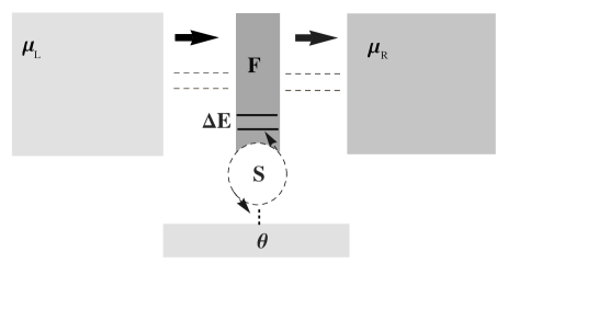
Figure 1: The global scheme of the model. Two-level system ${\bf F}$ transfers particles from a reservoir with chemical potential $\mu_{\rm L}$ to that with $\mu_{\rm R}$. The controller ${\bf S}$ tunes the energy difference $\Delta E$ of ${\bf F}$ and interacts with a bath at temperature $1/\theta$.

${\bf F}$ is a simple model for a trap (or adsorption center). It has two states ${\bf F}_{i}$ ($i=1,2$): an empty state ${\bf F}_{1}$ whose energy is $E_{1}$ and a filled state ${\bf F}_{2}$ with one particle and energy $E_{2}$. Hence each state has energy $E_{i}$ and carries $N_{i}$ particles($i=1,2$): $N_{2}=1$ and $N_{1}=0$; see Fig. 2. Without coupling to external reservoir(s), ${\bf F}$ will stay indefinitely in one of its states, since the energy and the particle number are conserved. Hence any change between the states of ${\bf F}$ is driven externally.

Let us first assume that ${\bf F}$ interacts with an equilibrium reservoir at chemical potential $\mu$ and temperature $T=1$ (this value of temperature is chosen conventionally, since temperature gradients will not play any role in our study). The stationary (time-independent) probabilities $\bar{p}_{i}^{\rm[eq]}$ of ${\bf F}_{i}$ ($i=1,2$) have the grand-canonical (equilibrium) Gibbsian form landau ; kampen

$$\bar{p}_{i}^{\rm[eq]}\propto e^{-E_{i}+\mu N_{i}}.$$ (1)

The relaxation of ${\bf F}$ towards its equilibrium state (1) can be described by the master equation kampen :

$$\dot{p}_{i}\equiv{{\rm d}p_{i}}/{{\rm d}t}={\sum}_{j}[\rho_{ij}p_{j}-\rho_{ji}p_{i}],\qquad i,j=1,2,$$ (2)

where $p_{i}$ ($p_{1}+p_{2}=1$) is the probability of ${\bf F}_{i}$ and $\rho_{i\not=j}$ is the transition rate ${\bf F}_{j}\to{\bf F}_{i}$. Since the bath is in equilibrium, $\rho_{i\not=j}$ hold the detailed balance condition:

$$\rho_{12}=e^{(E_{2}-E_{1})-\mu(N_{2}-N_{1})}\rho_{21}=e^{\Delta E-\mu}\rho_{21},$$ (3)

$$\Delta E\equiv E_{2}-E_{1}.$$ (4)

Eq. (3) ensures that the stationary state of (2) coincides with (1).

Without loss of generality we parametrize transition rates $\rho_{12}$ and $\rho_{21}$ as

$$\rho_{12}=\frac{1}{\tau}e^{\frac{1}{2}[\Delta E-\mu]},~{}~{}\rho_{21}=\frac{1}{\tau}e^{\frac{1}{2}[-\Delta E+\mu]},$$ (5)

where $\tau$ is the time-scale induced by the interaction with the reservoir. In (2), $\tau$ scales the running time (and hence the relaxation time), but does not appear in the equilibrium probabilities (1). Microscopic derivations of the master equation show that $\tau$ depends on the features of the reservoir (e.g. its energy spectrum), but can also depend on the internal parameter $\Delta Q=\Delta E-\mu$; see weiss and (25) below. Since $\Delta Q$ is the heat received or transferred to the reservoir, the time-scale $\tau$ has the global minimum at $\Delta Q=0$: it takes longer to transfer a larger amount of heat. This holds for all physical cases we are aware of.

II.2 Master equation for two reservoirs

In the equilibrium state (1) all currents nullify; this is the main message of the equilibrium state and it is ensured by the detailed balance condition (3) kampen .

We are interested by transport due to a chemical potential gradient. Hence we assume that ${\bf F}$ simultaneously couples with two equilibrium reservoirs (L and R) of energy and particles . Their temperatures are equal,

$$T_{\rm L}=T_{\rm R}=T=1,$$ (6)

but the chemical potentials are different

$$\mu_{\rm L}>\mu_{\rm R}.$$ (7)

${\bf F}$ will transport particles from L to R; see Fig. 2 and (15) below. Its dynamics is described by a master equation (2), but now once ${\bf F}$ couples simultaneously with L and R,

$$\rho_{ij}=\rho_{ij|{\rm L}}+\rho_{ij|{\rm R}},$$ (8)

where $\rho_{ij|{\rm L}}$ and $\rho_{ij|{\rm R}}$ are the transition rates driven by separate reservoirs rozenbaum . Since ${\rm L}$ and ${\rm R}$ are in equilibrium, $\rho_{ij|{\rm k}}$ satisfy detailed balance [cf. (3)]

$$\rho_{12|{\rm k}}=e^{\Delta E-\mu_{{\rm k}}}\rho_{21|{\rm k}},\qquad{\rm k}={\rm L},{\rm R}.$$ (9)

As (2) shows, ${\bf F}$ relaxes in time from any initial probability to the stationary (but generally non-equilibrium) probability

$$\bar{p}_{i}={\rho_{ij}}/{(\rho_{ij}+\rho_{ji})}.$$ (10)

If L and R are in mutual equilibrium ($\mu=\mu_{{\rm L}}=\mu_{{\rm R}}$), $\bar{p}_{i}$ reverts via (9) to the equilibrium (Gibbs) probability (1). We can apply the same parametrization as in (5)

$$\rho_{12|{\rm k}}=\frac{1}{\tau_{\rm k}}e^{\frac{1}{2}[\Delta E-\mu_{\rm k}\Delta N]},~{}~{}\rho_{21|{\rm k}}=\frac{1}{\tau_{\rm k}}e^{\frac{1}{2}[-\Delta E+\mu_{\rm k}\Delta N]},$$ (11)

where $\tau_{\rm k}$ is the time-scale of ${\bf F}-{\rm k}$ interaction (${\rm k}={\rm L},{\rm R}$). The discussion given after (5) now applies to $\tau_{\rm k}$ in separate. In particular, $\tau_{\rm k}$—as a function of $\Delta_{\rm k}Q=\Delta E-\mu_{\rm k}$ (heat received or transferred to the reservoir ${\rm k}$)—has the global minimum at $\Delta Q_{\rm k}=0$.

In contrast to the equilibrium situation, now the time-scales $\tau_{\rm k}$ will generally appear also in the stationary probability (10); see (18) below.

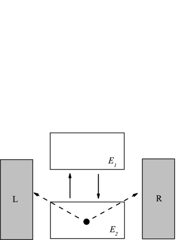
Figure 2: Two states of the functional degree of freedom ${\bf F}$; see section II.1 and II.2. The state ${\bf F}_{1}$ (${\bf F}_{2}$) is empty (filled with one particle) and has energy $E_{1}$ ($E_{2}$). The particle in ${\bf F}_{2}$ can move to one of the reservoirs (L or R) causing transition ${\bf F}_{2}\to{\bf F}_{1}$. The reverse transition ${\bf F}_{1}\to{\bf F}_{2}$ is due to catching a particle from one of the reservoirs. The mechanism of transporting particles from L to R is that a particle comes from L and then jumps to R; see (15).

II.3 Particle current

II.3.1 General definition

Our main target is the particle current: the mean number of particles entering to ${\bf F}$ per time-unit from the k-reservoir. To find the current, let us note that the time-derivative of the average number of particles

$$\frac{{\rm d}}{{\rm d}t}{\sum}_{i}N_{i}p_{i}={\sum}_{i}N_{i}\dot{p}_{i}={\sum}_{\rm k=L,R}J_{\rm k},$$ (12)

$$J_{\rm k}={\sum}_{ij}N_{i}[\rho_{ij|{\rm k}}\,p_{j}-\rho_{ji|{\rm k}}\,p_{i}],~{}{\rm k}={\rm L},{\rm R},$$ (13)

is a sum $J_{\rm L}+J_{\rm R}$ of two separate contributions. $J_{\rm k}$ is due to interaction with the reservoir ${\rm k}$, i.e. it is formed by the transition rates $\rho_{ij|{\rm k}}$ coming from the reservoir ${\rm k}$. These transitions rates satisfy the detailed balance with respect to the reservoir ${\rm k}$; see (8, 9). Since the particle number is conserved during the interactio of ${\bf F}$ with each reservoir, the contribution $J_{\rm k}$ to $\frac{{\rm d}}{{\rm d}t}{\sum}_{i}N_{i}p_{i}$ coming from the reservoir ${\rm k}$ is identified with the current of particles from the reservoir ${\rm k}$ seifert_review ; spohn . Then (12) expresses the conservation law .

Eqs. (2, 13) lead to

$$J_{\rm k}=\rho_{21|{\rm k}}\,p_{1}-\rho_{12|{\rm k}}\,p_{2},\qquad{\rm k}={\rm L},{\rm R},$$ (14)

where we recalled that $N_{2}=1$ and $N_{1}=0$. It should be intuitively clear from (14) that $J_{\rm k}$ is indeed the average number of particles entering from the reservoir ${\rm k}$: $\rho_{21|{\rm k}}\,p_{1}$ is (proportional to) the probability for ${\bf F}$ to make transition ${\bf F}_{1}\to{\bf F}_{2}$ induced by the reservoir ${\rm k}$ (hence ${\bf F}$ catches a particle from the reservoir ${\rm k}$). From this one subtracts the probability $\rho_{12|{\rm k}}\,p_{2}$ of the reverse event: the particle leaving from ${\bf F}$ to the reservoir ${\rm k}$.

II.3.2 Stationary situation

In the stationary (time-independent) situation $\bar{J}_{\rm L}+\bar{J}_{\rm R}=\frac{{\rm d}}{{\rm d}t}\sum_{i}N_{i}\bar{p}_{i}=0$; see (12, 13). As expected, there is only one independent current in the stationary situation. Using (10, 14) we get

$$\bar{J}_{\rm L}=\frac{\rho_{21|{\rm L}}\rho_{12|{\rm R}}-\rho_{12|{\rm L}}\rho_{21|{\rm R}}}{\rho_{12}+\rho_{21}}.$$ (15)

Eq. (15) has a transparent interpretation that explains the mechanism of the particle transport from L to R; see also Fig. 2 in this context. Indeed, $\rho_{21|{\rm L}}$ is (proportional to) the probability that ${\bf F}$ transits ${\bf F}_{1}\to{\bf F}_{2}$ under influence of L. This means that the particle in ${\bf F}$ came from L. Likewise, $\rho_{12|{\rm R}}$ is the probability that the particle will leave to R. Hence $\rho_{21|{\rm L}}\rho_{12|{\rm R}}-\rho_{12|{\rm L}}\rho_{21|{\rm R}}$ in (15) is (proportional to) the probability that the particle came from L and leaves to R minus the probability of the reverse sequence of events.

Eqs. (2–14) imply for the stationary values

$$\bar{J}_{\rm L}=\frac{\sinh[\frac{\mu_{\rm L}-\mu_{\rm R}}{2}]}{\tau_{\rm L}\cosh[\frac{\Delta E-\mu_{\rm R}}{2}]+\tau_{\rm R}\cosh[\frac{\Delta E-\mu_{\rm L}}{2}]},$$ (16)

$$\bar{p}_{1}=\left[1+e^{-\Delta E+l+\frac{\mu_{\rm L}+\mu_{\rm R}}{2}}\right]^{-1},\quad\bar{p}_{2}=1-\bar{p}_{1},$$ (17)

$$l\equiv\ln\left[({\tau_{\rm L}+\tau_{\rm R}e^{\frac{\mu_{\rm L}-\mu_{\rm R}}{2}}})\left/({\tau_{\rm R}+\tau_{\rm L}e^{\frac{\mu_{\rm L}-\mu_{\rm R}}{2}}})\right]\right.,$$ (18)

where $\Delta E$ is defined in (4).

Now $\bar{J}_{\rm L}\geq 0$ for $\mu_{L}\geq\mu_{\rm R}$: the stationary current is from the higher chemical potential to the lower one.

Note from (17) that provided that $l=0$, the stationary probability $\bar{p}_{1}$ of ${\bf F}$ has a Gibbsian form with the temperature $T=1$ and chemical potential $\frac{\mu_{\rm L}+\mu_{\rm R}}{2}$; $l=0$ is achieved under $\mu_{\rm L}=\mu_{\rm R}$ (overall equilibrium) or $\tau_{\rm L}=\tau_{\rm R}$. If the latter condition holds, $\frac{\mu_{\rm L}+\mu_{\rm R}}{2}$ is in between of the chemical potentials of the reservoirs ${\rm L}$ and ${\rm R}$; hence ${\bf F}$ is generally not in equilibrium with them, even when it has a Gibbsian form. The fact of having a Gibbsian form—that physically means the existence of a local equilibrium—will be seen below to have important consequences.

II.4 Maximization of the particle current

We want to have the largest $\bar{J}_{\rm L}$ for given $\mu_{\rm L}$ and $\mu_{\rm R}$, because this means the optimal functioning of the matter-transporting machine. We start with a general premise that the current $\bar{J}_{\rm L}$ should be finite. This implies from (16) two natural constraints [${\cal T}$ is a constant, k=L,R]:

$$\tau_{\rm k}\geq{\cal T},$$ (19)

i.e. time-scales cannot be too short. The largest $\bar{J}_{\rm L}$ for given $\mu_{\rm L}$, $\mu_{\rm R}$ and (19) is obtained when we maximize (16) with all the three involved parameters $\tau_{\rm L}$, $\tau_{\rm R}$, $\Delta E$ being independent under conditions (19):

$$\bar{J}_{\rm L}^{*}\equiv\max_{\tau_{\rm k},\Delta E}\,[\bar{J}_{\rm L}]=\frac{1}{{\cal T}}\sinh[\frac{\mu_{\rm L}-\mu_{\rm R}}{4}],$$ (20)

which is reached for the optimal values

$$\tau^{*}_{\rm L}=\tau^{*}_{\rm R}={\cal T},\qquad\Delta E^{*}=\bar{\mu}\equiv(\mu_{\rm L}+\mu_{\rm R})/2.$$ (21)

Eq. (20) is got as follows. We maximize $\bar{J}_{\rm L}$ over $\tau_{\rm L}$ and $\tau_{\rm R}$ and obtain the first condition in (21). Next we maximize over $\Delta E$.

Here are the implications of (20–21).

1. The optimal $\tau^{*}_{\rm k}$ are fixed by the constraints. In contrast, $\Delta E^{*}$ depends on the environment (reservoirs). The optimality condition $\tau_{\rm L}=\tau_{\rm R}$ implies $l=0$ from (18). Hence the stationary probabilities $\bar{p}_{i}$ for ${\bf F}_{i}$ have the Gibbsian form with chemical potential (21); see (17) and the discussion after (18). This consequence of the current maximization is one the main causes of our results below.

2. The machine performing optimally in one environment will be sub-optimal in another. Indeed, let the parameters be fixed at their optimal values (21), and the chemical potentials are slowly changed as

$$\mu_{\rm L}\to\mu^{\prime}_{\rm L},~{}~{}\,\mu_{\rm R}\to\mu^{\prime}_{\rm R},~{}~{}\,\mu^{\prime}_{\rm L}>\mu^{\prime}_{\rm R},~{}~{}\,\bar{\mu}\to\bar{\mu}^{\prime}\equiv\bar{\mu}+\delta,\,$$ (22)

where $\delta=\frac{1}{2}(\mu^{\prime}_{\rm L}-\mu_{\rm L}+\mu^{\prime}_{\rm R}-\mu_{\rm R})$.

The stationary current in the new situation (22) is

$$\bar{J}_{\rm L}[\mu^{\prime}_{\rm L},\mu^{\prime}_{\rm R}]={\bar{J}_{\rm L}^{*}[\mu^{\prime}_{\rm L},\mu^{\prime}_{\rm R}]}/{\cosh[\,\frac{\delta}{2}\,]},$$ (23)

where $\bar{J}_{\rm L}^{*}[\mu^{\prime}_{\rm L},\mu^{\prime}_{\rm R}]$ is the optimal current in the new environment; see (21, 16). For $|\delta|\gg 1$ we get ${\bar{J}_{\rm L}[\mu^{\prime}_{\rm L},\mu^{\prime}_{\rm R}]}\ll{\bar{J}_{\rm L}^{*}[\mu^{\prime}_{\rm L},\mu^{\prime}_{\rm R}]}$: the current becomes suboptimal for any sizable environmental change. If the chemical potential difference is conserved, $\mu^{\prime}_{\rm L}-\mu^{\prime}_{\rm R}\approx\mu_{\rm L}-\mu_{\rm R}$, the current will decrease from its old value: ${\bar{J}_{\rm L}[\mu^{\prime}_{\rm L},\mu^{\prime}_{\rm R}]}\ll{\bar{J}_{\rm L}^{*}[\mu_{\rm L},\mu_{\rm R}]}$.

3. The formal reason of this fragility is that the optimal $\Delta E^{*}$ depends on the environment. Its physical reason is that ${\bf F}$ has to perform equally well two complementary things: to bind and release. To illustrate this point, recall that $N_{2}=1$, $N_{1}=0$ and assume in (21, 11):

$$\tau_{\rm L}=\tau_{\rm R}={\cal T}=1.$$ (24)

Then the binding transition ${\bf F}_{1}\to{\bf F}_{2}$ is driven mainly by the L reservoir, $\rho_{21|{\rm L}}>\rho_{21|{\rm R}}$, while the releasing transition ${\bf F}_{2}\to{\bf F}_{1}$ is driven mainly by R: $\rho_{12|{\rm R}}>\rho_{12|{\rm L}}$ (this is why ${\bf F}$ transports particles from L to R). In the optimal regime both $\rho_{21|{\rm L}}$ and $\rho_{12|{\rm R}}$ should be possibly large. Hence they are equal: $\rho_{21|{\rm L}}=\rho_{12|{\rm R}}=e^{\frac{1}{4}(\mu_{\rm L}-\mu_{\rm R})}$, i.e. ${\bf F}$ binds and releases the particle equally well. Now after the environmental change (22): $\rho_{21|{\rm L}}/\rho_{12|{\rm R}}=e^{{\delta}/{2}}$. Thus for $\delta>0$ ($\delta<0$) the current is sub-optimal, since ${\bf F}$ binds the particle better (worse) than releases it.

4. Our model relates to inhomogeneous catalysis. Any catalysis facilitates the spontaneous transfer of reacting molecules from a higher to a lower chemical potential chem . During an inhomogeneous catalysis the reactants are bound strongly to an active center of the catalysing surface, so that the reaction can proceed. But the reaction products should be weakly bound to the center, so that they are easily released making the center ready for a new reaction. This complementarity between binding and releasing is essential for any good catalyst; e.g. silver and tungsten are both not good catalysis for organic molecules: silver binds reactants too weakly, while tungsten binds the products too strongly chem .

Another situation, where binding and releasing are simultaneously important is the oxygen transport by mammal erythrocytes. They are periodically removed from the blood, since they cease to perform well one of these functions, e.g., they bind oxygen too strongly trincher .

5. Recall that in deriving (20) we assumed that the current $\bar{J}_{\rm L}$ can be maximized over independent parameters $\tau_{\rm L}$, $\tau_{\rm R}$, $\Delta E$; see also 2, where this assumption was used implicitly. While this leads to the largest value of $\bar{J}_{\rm L}$—in the sense that any relation between the three parameters can only reduce the optimal value (20)—it is still possible that $\tau_{\rm k}$ does depend on $\Delta Q_{\rm k}=\Delta E-\mu_{\rm k}$, e.g. in the activated transport weiss

$$\tau_{\rm k}=\exp[v_{\rm k}+\frac{1}{2}|\Delta Q_{\rm k}|],$$ (25)

where $v_{\rm k}$ is the barrier height. We now show that in the linear regime $\mu_{\rm L}\approx\mu_{\rm R}$ we can recover the same conclusions as above without assuming that $\tau_{\rm k}$ does not depend on $\Delta Q_{\rm k}$.

In the linear regime we put $\mu_{\rm L}=\mu_{\rm R}=\bar{\mu}$ everywhere besides $\sinh[\frac{\mu_{\rm L}-\mu_{\rm R}}{2}]\approx\frac{\mu_{\rm L}-\mu_{\rm R}}{2}$ in (16):

$$\bar{J}_{\rm L}=\frac{\mu_{\rm L}-\mu_{\rm R}}{2[\tau_{\rm L}(\Delta Q)+\tau_{\rm R}(\Delta Q)]\cosh[\frac{\Delta E-\bar{\mu}}{2}]},$$ (26)

where $\tau_{\rm L}$ and $\tau_{\rm R}$ are functions of $\Delta Q=\Delta E-\bar{\mu}$ weiss . They have global minima at $\Delta Q=0$ [see our discussion after (5)]. In the linear regime the stationary probabilities of ${\bf F}$ are naturally Gibbsian, since $l=0$ in (17, 18).

Maximizing (26) over $\Delta E$ we get $\bar{J}_{\rm L}^{*}=\frac{\mu_{\rm L}-\mu_{\rm R}}{2[\tau_{\rm L}(0)+\tau_{\rm R}(0)]}$ reached for $\Delta E^{*}=\bar{\mu}$. In the linear regime these agree with (20). Also, we reproduce the conclusions of 1-4 by keeping the dependence of $\tau_{\rm k}$ on $\Delta Q$. Note that the changes in (22) should respect the linear regime: $\mu^{\prime}_{\rm L}-\mu^{\prime}_{\rm R}\approx\mu_{\rm L}-\mu_{\rm R}\approx 0$.

6. We aimed to show that in the linear regime our conclusions on the current optimality and its fragility apply more generally. We do not assume the linear regime for the rest of this paper. Below we set $\tau_{\rm L}=\tau_{\rm R}={\cal T}$, because this maximizes $\bar{J}_{\rm L}$ with all other parameters being fixed. For technical simplicity we from now on put ${\cal T}=1$ [cf. (24)].

III Structural degree of freedom

III.1 Master equation

We discussed in 2 that the environmental changes (22) diminish the optimal current. If our machine is supposed to work in such an uncertain environment, the only possibility to ensure its optimal functioning is to assume that its structure ${\bf S}$ changes and adjusts the energy difference to $\Delta E=\bar{\mu}^{\prime}$ after each environmental change $\bar{\mu}\to\bar{\mu}^{\prime}$; see (22). Then the current is maximal under each environment. To account for structural changes we thus introduce a controller degree of freedom ${\bf S}$, with states $\{{\bf S}^{\alpha}\}_{\alpha=1}^{K}$; see Fig. 3. We shall demand that ${\bf S}$ is slower than ${\bf F}$ and that it does not couple directly to the changing environment.

Let $p_{i}^{\alpha}$ and $E_{i}^{\alpha}$ be, respectively, the joint probability and energy of ${\bf S}^{\alpha}{\bf F}_{i}$. Since ${\bf S}$ does not couple to particle reservoirs L and R, each state ${\bf S}^{\alpha}{\bf F}_{i}$ carries the number of particles $N_{i}$ that does not depend on $\alpha$; see Fig. 3. Hence the ${\bf S}-{\bf F}$ coupling goes only via the energies $E_{i}^{\alpha}$.

The dynamics of ${\bf S}$ is driven by a thermal bath at a temperature $1/\theta$; see Fig. 1. It will be seen below that the adaptation makes necessary for the baths of ${\bf F}$ and ${\bf S}$ to be different. Hence we assume that the baths of ${\bf S}$ and ${\bf F}$ are independent, and the general master equation $\dot{p}_{i}^{\alpha}={\sum}_{j\gamma}[R_{ij}^{\alpha\gamma}p_{j}^{\gamma}-R_{ji}^{\gamma\alpha}p_{i}^{\alpha}]$ for ${\bf S}+{\bf F}$ reduces to

$$\dot{p}_{i}^{\alpha}={\sum}_{j}[\rho_{ij}^{\alpha}p_{j}^{\alpha}-\rho_{ji}^{\alpha}p_{i}^{\alpha}]+\epsilon{\sum}_{\gamma}[\omega^{\alpha\gamma}_{i}p_{i}^{\gamma}-\omega^{\gamma\alpha}_{i}p_{i}^{\alpha}],$$ (27)

where $\omega^{\alpha\gamma}_{i}$ and $\rho_{ij}^{\alpha}=\sum_{{\rm k}={\rm L},{\rm R}}\rho_{ij|{\rm k}}^{\alpha}$ are the rates of transitions ${\bf F}_{i}{\bf S}^{\gamma}\to{\bf F}_{i}{\bf S}^{\alpha}$ and ${\bf F}_{j}{\bf S}^{\alpha}\to{\bf F}_{i}{\bf S}^{\alpha}$, respectively. $\epsilon$ is the ratio between the time-scales of ${\bf F}$ and ${\bf S}$. The detailed balance for $\rho_{ij|{\rm k}}^{\alpha}$ reads [cf. (11)]

$$\rho_{12|{\rm k}}^{\alpha}=e^{\frac{1}{2}(E^{\alpha}_{2}-E^{\alpha}_{1}-\mu_{{\rm k}})},~{}~{}\rho_{21|{\rm k}}^{\alpha}=1/\rho_{12|{\rm k}}^{\alpha},$$ (28)

where in (28) we used the settings (24); recall 6 in section II.4.

The detailed balance condition for $\omega^{\alpha\gamma}_{i}$ is written down by analogy to (11)

$$\omega_{i}^{\alpha\gamma}=e^{\frac{1}{2}B^{\alpha\gamma}_{i}+\frac{\theta}{2}(E^{\gamma}_{i}-E^{\alpha}_{i})},\quad B^{\alpha\gamma}_{i}=B^{\gamma\alpha}_{i},$$ (29)

where $B^{\alpha\gamma}_{i}$ relates to the inverse time-scale, and $\theta$ is the inverse temperature of the bath of ${\bf S}$ [recall (6) in this context].

Figure 3: The joint states of functional degree ${\bf F}$ and the structural degree ${\bf S}$. For simplicity it is assumed that both ${\bf F}$ and ${\bf S}$ can have two separate states (${\bf F}_{1},{\bf F}_{2}$ and ${\bf S}^{1},{\bf S}^{2}$, respectively); recall Fig. 2. Hence there are four states ${\bf F}_{i}{\bf S}^{\alpha}$ (of ${\bf F}+{\bf S}$) with energies $E_{i}^{\alpha}$. The transitions ${\bf F}_{i}{\bf S}^{\alpha}\to{\bf F}_{i}{\bf S}^{\beta}$, ${\bf F}_{i}{\bf S}^{\alpha}\to{\bf F}_{j}{\bf S}^{\alpha}$ take place between states having one common index; see (27). This is due to the fact that the reservoirs that drive the transitions are independent from each other.

III.2 Time-scale separation

It is generally understood that control processes in biology involve time-scale separations between controlling and functional degrees of freedom; see roj ; gun for reviews . In line with this, we assume that ${\bf S}$ is much slower than ${\bf F}$ for $\epsilon\to 0$. One introduces in (27) the conditional probability $p_{i|\alpha}$ defined via $p_{i|\alpha}p^{\alpha}=p_{i}^{\alpha}$, and notes that in $\dot{p}_{i}^{\alpha}=\dot{p}^{\alpha}p_{i|\alpha}+p^{\alpha}\dot{p}_{i|\alpha}$ we have $p^{\alpha}\dot{p}_{i|\alpha}={\cal O}(1)$ and $\dot{p}^{\alpha}p_{i|\alpha}={\cal O}(\epsilon)$ a+n . Hence $\dot{p}_{i|\alpha}$ and $\dot{p}^{\alpha}$ decouple:

$$\dot{p}_{i|\alpha}={\sum}_{j\not=i}[\,\rho_{ij}^{\alpha}p_{j|\alpha}-\rho_{ji}^{\alpha}p_{i|\alpha}\,],$$ (30)

$$\dot{p}^{\alpha}=\epsilon{\sum}_{\gamma}[\Omega^{\alpha\gamma}p^{\gamma}-\Omega^{\gamma\alpha}p^{\alpha}],\,\,\Omega^{\alpha\gamma}={\sum}_{i}\omega^{\alpha\gamma}_{i}\,p_{i|\gamma}.$$ (31)

Eq. (30) describes the evolution of ${\bf F}$ for short times when ${\bf S}$ is fixed in its state ${\bf S}^{\alpha}$. Then ${\bf F}$ relaxes to its conditional equilibrium$\bar{p}_{1|\alpha}=\frac{\rho_{12}^{\alpha}}{\rho_{12}^{\alpha}+\rho_{21}^{\alpha}}=[1+e^{-\Delta E^{\alpha}+\bar{\mu}}]^{-1}$, where $\Delta E^{\alpha}=E^{\alpha}_{2}-E^{\alpha}_{1}$; see (10, 17). Since this relaxation happens faster than ${\bf S}$ changes, for describing the dynamics of ${\bf S}$ one can replace in (31):

$$\Omega^{\alpha\gamma}\to\bar{\Omega}^{\alpha\gamma}={\sum}_{i}\omega^{\alpha\gamma}_{i}\,\bar{p}_{i|\gamma}.$$ (32)

Then (31) becomes a Markov master equation for ${\bf S}$: the future of ${\bf S}$ is determined by its own present state only. ${\bf F}$ influences ${\bf S}$ indirectly via the transition rates $\bar{\Omega}^{\alpha\gamma}$.

Since most of the time ${\bf F}$ is in its stationary situations corresponding to a fixed ${\bf S}^{\alpha}$, the functioning of the machine is described by the current $\bar{J}^{\alpha}_{\rm L}$ in the states ${\bf S}^{\alpha}$ and the stationary probability $\bar{p}^{\alpha}$ of ${\bf S}^{\alpha}$ found from (31, 32). This is the main consequence of the time-scale separation.

Using (17) with $l=0$ [see (31)] we get from (32, 29):

$$\frac{\bar{\Omega}^{\alpha\beta}}{\bar{\Omega}^{\beta\alpha}}=e^{\theta(E_{1}^{\beta}-E_{1}^{\alpha})}\,\frac{1+e^{\bar{\mu}-\Delta E^{\alpha}}}{1+e^{\bar{\mu}-\Delta E^{\beta}}}\,\,\times$$

$$\frac{1+e^{b^{\alpha\beta}+\frac{\theta}{2}(\Delta E^{\beta}-\Delta E^{\alpha})-\Delta E^{\beta}+\bar{\mu}}}{1+e^{b^{\alpha\beta}+\frac{\theta}{2}(\Delta E^{\alpha}-\Delta E^{\beta})-\Delta E^{\alpha}+\bar{\mu}}},$$ (33)

$$\Delta E^{\alpha}\equiv E_{2}^{\alpha}-E_{1}^{\alpha},\quad b^{\alpha\beta}\equiv(B_{2}^{\alpha\beta}-B_{1}^{\alpha\beta})/2.$$ (34)

At this stage we need to specify the transition rates $\omega_{i}^{\alpha\gamma}$, because on one hand we want to have a non-trivial structure of ${\bf S}$ (including the possibility of taking $K\to\infty$), while on the other hand we want to get $\bar{p}^{\alpha}$ explicitly. We thus choose to work with the birth-death model for ${\bf S}$ kampen : the states $\{{\bf S}^{\alpha}\}_{\alpha=1}^{K}$ with energies $\{E^{\alpha}_{i}\}_{\alpha=1}^{K}$ form a one-dimensional chain. In (27–31) we allow transitions only between neighbouring states: ${\bf S}^{\alpha}\leftrightarrows{\bf S}^{\alpha+1}$, $\alpha=1,\ldots,K-1$. Then the stationary probability of ${\bf S}$ reads from (31, 32)

$$\bar{p}^{\alpha}=\bar{p}^{1}{\prod}_{\gamma=1}^{\alpha-1}\left(\bar{\Omega}^{\gamma+1,\,\gamma}/\bar{\Omega}^{\gamma,\,\gamma+1}\right),~{}~{}\alpha=2,\ldots,K,$$ (35)

where $\bar{p}^{1}$ is determined from ${\sum}_{\alpha=1}^{K}\bar{p}^{\alpha}=1$.

IV Adaptation

IV.1 Definition of adaptation

The intuitive notion of adaptation is that this is a change in the system compensating environmental effects. The general definition of adaptation was attempted in literature several times and led to interesting discussions; see formal ; taivo for reviews . But within general definitions some important aspects of adaptation are left open, the main of them is why (let alone how) the system is going to compensate environmental effects .

In our situation the adaptation is a structural change needed for compensating parametric environmental uncertainty which is detrimental to the machine function: transporting particles with the maximal current [see (23) and the discussion around].

Let the environment changes as in (22), and $\bar{\mu}$ can assume any value from a set ${\cal M}$. It resides in each of its states with a fixed $\bar{\mu}$ for a sufficiently long time so that ${\bf F}$ and ${\bf S}$ do have enough time to relax to the stationary probabilities $\bar{p}^{\alpha}$ and $\bar{p}_{i|\alpha}$. We require that the machine functions optimally, $\bar{J}_{\rm L}(\bar{\mu})=\bar{J}^{*}_{\rm L}$, in each environment: the probability $\bar{p}^{\alpha}$ of the structural state with $\Delta E^{\alpha}=\bar{\mu}$ [see (21, 24)] is maximized for each $\bar{\mu}\in{\cal M}$, i.e. the probabilities of all other states are suppressed in the sense discussed below. The choice between the optimal structural states is done autonomously: after $\bar{\mu}$ changes from one value to another (or goes back to its older value), ${\bf F}+{\bf S}$ relax to a new stationary regime, where the structural state with the largest current dominates. Recall that ${\bf S}$ does not feel the parameter $\bar{\mu}$ directly, because it does not interact directly with the particle reservoirs; it feels $\bar{\mu}$ only indirectly due to interaction with ${\bf F}$. Hence the changes of ${\bf S}$ are driven by ${\bf F}$.

IV.2 Continuum limit

We assume that ${\cal M}$ is a finite real interval. There should be a correspondence between $\{{\bf S}\}_{\alpha=1}^{K}$ and environmental states; thus to have adaptation for this case we need to make $\alpha$ a continuous variable $x$ and to take in (33–35) the continuum limit: $K\to\infty$,

$$E^{\alpha+1}_{i}-E^{\alpha}_{i}=E_{i}(x+\frac{1}{K})-E_{i}(x)=\frac{1}{K}\partial_{x}E_{i}(x),$$ (36)

$$b^{\alpha,\alpha+1}=b(x,x+\frac{1}{K})=b(x)+\frac{1}{K}\partial_{y}b(x,y)|_{y=x},$$ (37)

where $b(x)=b(x,x)$ and where the continuous variable $x$ changes in an interval: $x\in[L_{1},L_{2}]$. Thus the stationary probability of ${\bf S}$ (which is now a probability density due to the continuum limit) depends on three functions $E_{i}(x)$ and $b(x)$. These functions look arbitrary, but we show below that they are fixed from the adaptation condition.

In the continuum limit the sums over $\gamma$ in (35) can be replaced by integrals. As shown in Appendix A, the stationary probability of ${\bf S}$ then reads from (35) [$A^{\prime}(x)\equiv\partial_{x}A(x)$]

$$\bar{p}(x)=\exp[-\Psi(x)]/Z,$$ (38)

$$\Psi^{\prime}(x)=\theta f^{\prime}(x)+(\theta-1)\phi(x)[f^{\prime}(x)-E_{1}^{\prime}(x)],$$ (39)

$$f(x)=-\ln[\,e^{-E_{1}(x)}+e^{-E_{2}(x)+\bar{\mu}}\,],$$ (40)

$$\phi(x)=[\,e^{b(x)}-1\,]\,[\,e^{b(x)+\bar{\mu}-E_{2}(x)+E_{1}(x)}+1\,]^{-1},$$ (41)

where $Z$ in (38) is deduced from $\int_{L_{1}}^{L_{2}}{\rm d}x\,\bar{p}(x)=1$. In (40), $f(x)$ is the free energy of ${\bf F}$ calculated at a fixed $x$; see (17) and a+n . The second term in (39) is due to different temperatures of ${\bf S}$ and ${\bf F}$ ($\theta\not=1$) and the dependence of the times-scales of ${\bf S}$ on ${\bf F}$ ($b(x)\not=0$); see (29, 34).

For adaptation it is necessary that for any $\bar{\mu}\in{\cal M}$, $\bar{p}(x)$ in (38) has a unique and sharp maximum at $x=\hat{x}(\bar{\mu})$ with [cf. (21, 24)]:

$$\Delta E(\hat{x}(\bar{\mu}))\equiv E_{2}(\hat{x}(\bar{\mu}))-E_{1}(\hat{x}(\bar{\mu}))=\bar{\mu}.$$ (42)

Then $\hat{x}(\bar{\mu})$ will be the most probable value of $x$. Two conditions for $\hat{x}(\bar{\mu})$ to be a local maximum of $\bar{p}(x)$ are $\Psi^{\prime}(\hat{x}(\bar{\mu}))=0$ and $\Psi^{\prime\prime}(\hat{x}(\bar{\mu}))>0$. Working out $\Psi^{\prime}(\hat{x}(\bar{\mu}))=0$ and using (42) we get

$$\frac{e^{b(\hat{x}(\bar{\mu}))}-1}{e^{b(\hat{x}(\bar{\mu}))}+1}=\frac{\theta}{1-\theta}\,\,\frac{E^{\prime}_{1}(\hat{x}(\bar{\mu}))+E^{\prime}_{2}(\hat{x}(\bar{\mu}))}{E^{\prime}_{2}(\hat{x}(\bar{\mu}))-E^{\prime}_{1}(\hat{x}(\bar{\mu}))}.$$ (43)

This relation is supposed to hold for all $\bar{\mu}\in{\cal M}$, and since functions $E_{1,2}(x)$ and $b(x)$ do not depend on $\bar{\mu}$— because, in particular, ${\bf S}$ does not interact with the particle reservoir— (43) holds in a dense set of $x$. Once $E_{1}(x)$, $E_{2}(x)$ and $b(x)$ are assumed to be smooth functions of $x$, (43) will hold for all $x\in[L_{1},L_{2}]$   ; it defines a functional relation between $E_{1}(x)$, $E_{2}(x)$ and $b(x)$:

$$\frac{e^{b(x)}-1}{e^{b(x)}+1}=\frac{\theta}{1-\theta}\,\,\frac{E^{\prime}_{1}(x)+E^{\prime}_{2}(x)}{E^{\prime}_{2}(x)-E^{\prime}_{1}(x)}.$$ (44)

We work now out $\Psi^{\prime\prime}(x)$ using (44) and put there (42):

$$\Psi^{\prime\prime}(\hat{x}(\bar{\mu}))=-\frac{[\Delta E^{\prime}(\hat{x}(\bar{\mu}))]^{2}}{4}\times$$

$$\left[\,\theta+(1-\theta)\left[\frac{e^{b(\hat{x}(\bar{\mu}))}-1}{e^{b(\hat{x}(\bar{\mu}))}+1}\right]^{2}\,\right].$$ (45)

We need $\theta<0$, i.e. a negative-temperature state of ${\bf S}$; otherwise $\hat{x}(\bar{\mu})$ is a minimum of $p(\hat{x}(\bar{\mu}))$, not maximum . We now set $b(x)=0$, because then any $\theta<0$ will suffice for adaptation; otherwise, $\theta$ has to be smaller than certain negative value. Eq. (44) under $b(x)=0$ implies $E^{\prime}_{1}(x)=-E^{\prime}_{2}(x)$. We shall see in section V that setting $b(x)=0$ appears to be optimal from the viewpoint of reducing fluctuations of $x$ around its most probable value. Recall from (34, 37) the physical meaning of the condition $b(x)=0$: the time-scale of ${\bf S}$ does not depend on the state of ${\bf F}$.

We conclude that the adaptation requires a negative temperature $\theta<0$ for ${\bf S}$. This condition holds as well when the environmental chemical potentials (and hence ${\bf S}$) assume a finite number of values; see Appendix D. After bringing an explicit example of adaptation, we continue with clarifying the generality of the $\theta<0$ condition (section IV.4) and its physical meaning (section IV.5).

IV.3 An example

Let us at this point stop the general reasoning and bring an explicit example of above construction (38–45): $E_{i}(x)=a_{i}x$ for $i=1,2$ is linear function of $x$ with its slope $a_{i}$ dependent on $i$. For a fixed $i$, $E_{i}(x)$ as a function of $x$ is a potential energy. This potential energy is not confining, but it is not a problem, since we anyhow restricted the allowed range of $x$: $x\in[L_{1},L_{2}]$. Now requiring $a_{1}=-a_{2}$ leads to $b(x)=0$; see (38–41, 44). The stationary probability of ${\bf S}$ reads from (38–41)

$$\bar{p}(x)\propto(\cosh[a_{2}x-\frac{\bar{\mu}}{2}])^{-|\theta|}.$$ (46)

The most probable value of $x$ is $\frac{\bar{\mu}}{2a_{2}}$, condition (42) is ensured, and the interval of allowed values of $\bar{\mu}$ is

$${\cal M}=2a_{2}\times[L_{1},L_{2}].$$ (47)

Note that the range ${\cal M}$ of $\bar{\mu}$ over which the adaptation occurs is finite and enters into the hardwire of ${\bf S}+{\bf F}$ as an apriori knowledge on the environment. ${\cal M}$ is finite due to the fact that ${\bf S}$ interacts with a negative-temperature bath: if the range of $x$ is not finite, such an interaction will lead to instability; see section IV.5 and ramsey ; butko ; brunner .

IV.4 Le Chatelier principle

Here we argue that the necessary condition $\theta<0$ for the adaptation is more general that the above derivation may suggest.

For $b(x)=0$ we get from (38–41) that $\Psi(x)=\theta f(x)$, where $f(x)$ is the free energy of ${\bf F}$ calculated for a fixed slow variable $x$. The joint probability of ${\bf F}+{\bf S}$ is then

$$p_{i}(x)\propto e^{\theta f(x)}p_{i|x},$$ (48)

where $p_{i|x}$ (as a function of $i$ for a fixed $x$) has a Gibbsian form; see (17, 21) and recall that in the optimal regime $\tau_{\rm L}=\tau_{\rm R}$. Eq. (48) for $p_{i}(x)$ implies the time-scale separated two-temperature system, which admits a consistent thermodynamic description despite the fact that the temperatures of ${\bf S}$ and ${\bf F}$ can be very different a+n . For such a system, the fact that the adaptation requires $\theta<0$ is deduced from the generalized Le Chatelier principle: $\theta<0$ is necessary that perturbations of the chemical potential do not amplify in time; see Appendix B.

IV.5 Negative temperature states

Let us discuss in more detail the features of negative-temperature states.

– They maximize (not minimize) the average energy for a fixed entropy ramsey ; butko ; brunner .

– They thus store energy: a cyclic external field can extract work from them ramsey ; butko . Such states are autonomous sources of work brunner .

– To support $\theta<0$, ${\bf S}$ needs to have a bounded phase-space ramsey ; butko ; brunner , as already assumed .

– Negative temperatures are higher than positive ones, since heat flows from lower inverse temperature to the larger one ramsey ; butko ; brunner . This implies that the energy stored in ${\bf S}$ due to $\theta<0$ will constantly flow to the bath of ${\bf F}$ with the rate proportional to $\epsilon$ [see (31] tending to dissipate the stored energy. This current is calculated in Appendix D.2. Due to assumed $\epsilon\ll 1$, it is smaller than the particle current $\bar{J}_{\rm L}$ in (16).

– One should distinguish between population inversion (there are at least two energy levels such that the higher energy level is more populated than the lower one) and a negative-temperature state of a many-level system, where in every pair of energy levels the higher energy level is more populated. These two notions are equivalent for a two level system, but generally they are different. A pair of energy levels with population inversion suffices for (necessarily imperfect) adaptation, if one can restrict ${\bf S}$ to those levels, i.e. neglect transitions for higher energy levels; see Appendix D. However, in that case the adaptation is necessarily imperfect, i.e. there is no limit, where the probability of the undesired structural states can be made arbitrary small. We focussed in section IV.2 on the negative-temperature state of a many-level system, because it does have a limit, where the adaptation can be made perfect; see section V below.

– States with population inversion can be prepared by pumping the system to higher energy levels; see butko for an extensive review of these methods. This includes not only lasers and masers, but also macroscopic magnetic moments, rotators, dipoles etc butko . It is also possible to prepare a population inversion via two weakly coupled systems held at different positive temperatures brunner .

– Many-body states with a negative temperature are well known and were experimentally realized for discrete and localized degrees of freedom such as the spin of nuclei or atoms oja ; butko . One scenario of their realization and observation is a microcanonic state of a many-spin system in the regime, where the number of available states decreases with increasing the energy oja ; karen . Negative-temperature states were also experimentally realized for motional states of cold atoms cold , where the energy spectrum of the negative-temperature carrying degrees of freedom is continuous, but bounded (similar to our example in section IV.2).

– There are complex materials held in metastable states that—without being properly negative-temperature—behave like negative-temperature states with respect to external variations ban .

– Living organisms are capable of being autonomous sources of work (the work is done, e.g. for preventing their relaxation to equilibrium). Hence they store energy at least via population inversion . This fact is well understood in biological thermodynamics bauer ; clare ; trincher_d ; kauffman ; voe and was employed in a definition of life kauffman ; see section VII.2 for more details.

V Fluctuations

We return to the stationary probability density $\bar{p}(x)$ of ${\bf S}$; see (38). Assume that the maximum $\hat{x}(\bar{\mu})$ of $\bar{p}(x)$ is unique. There are local fluctuations around that maximum, since $\bar{p}(x)$ is not a delta-function centered at $\hat{x}(\bar{\mu})$. Thus there are intrinsic fluctuations of $x$, and thus of $\Delta E(x)$, even for an environment with a fixed $\bar{\mu}$. For $x\approx\hat{x}(\bar{\mu})$, (38) amounts to

$$\bar{p}(x)\propto\exp[-\frac{1}{2}|\Psi^{\prime\prime}(\hat{x}(\bar{\mu}))|(\hat{x}(\bar{\mu})-x)^{2}],$$ (49)

the standard deviation of $x$ is $\sigma_{x}=1/\sqrt{|\Psi^{\prime\prime}(\hat{x})|}$. We need to consider fluctuations of $\Delta E(x)$, since ${\bf F}$ feels $x$ only via $\Delta E(x)$. If $\sigma_{x}$ is small, the standard deviation of $\Delta E(x)$ around $\bar{\mu}$ is

$$\sigma=|\Delta E^{\prime}(\hat{x})|\sigma_{x}={2}/{\sqrt{|\theta|}},$$ (50)

where we used (45); recall that we set $b(x)=0$, this is also optimal from the viewpoint of reducing $\sigma$.

Now the only possibility of $\sigma\to 0$ is to take $\theta\to-\infty$, i.e. a vanishing entropy of ${\bf S}$ due to a large amount of stored energy. There are two general methods of fighting against fluctuations: reducing the environmental noise as such (e.g. cooling the environment), or putting the system under a strong confining potential. The second method does not work in our situation, since it appears that the strong potential cannot be adaptive.

Thus, the adaptation is generally imperfect, because even at a fixed environment (for a fixed $\bar{\mu}$), $\Delta E$ will fluctuate on characteristic times of ${\bf S}$. The imperfect adaptation is useful only if the environmental changes are wide enough; otherwise the same machine with a fixed optimal structure tuned to the average environment will have a larger average current. This point is worked out in Appendix C.

VI Alternative set-ups of adaptation

To get the proper perspective on the obtained results we briefly mention certain extensions of the basic set-up.

Above we required that the set ${\cal M}$ of environmental values of $\bar{\mu}$ is dense. The same limitations (negative temperature and structural fluctuations) are obtained when the environment assumes a finite number of values; see Appendix D. But here fluctuations are finite even for $\theta\to-\infty$.

Another set-up is to allow ${\bf S}$ to interact directly with the uncertain environment [see Appendix E]. This is done naturally assuming that different states ${\bf F}_{i}{\bf S}^{\alpha}$ have different particle numbers $N^{\alpha}_{i}$. The above limitations are then absent: even the two-state ${\bf S}$ (in face of a binary environment) can ensure perfect adaptation in the isothermal situation $\theta=1$. In this set-up ${\bf S}$ becomes an external sensor for the machine. (This is sometimes called feed-forward scenario of adaptation in contrast to the previous scenario that works via feedback to ${\bf F}$: ${\rm\bf environment}\to{\bf F}\to{\bf S}\to{\bf F}$.) Hence no stored energy is needed and no fluctuations at the constant environments are necessarily present. (Fluctuations may still be present due to various non-idealities.) The drawback of this set-up is that it demands a specific structure-environment interaction that has to designed anew for every new environment. Put differently, the above thermodynamic costs are necessary for ensuring the autonomous character of the adaptation.

Yet a different set-up is to relax the optimality condition demanding instead the stabilization (constancy) of the current on the face of environmental changes at some sub-optimal value; the above limitations are then also weakened. The conceptual problem with relaxing the optimality condition is that then the very adaptation may easily become useless: who wants to keep a machine that does not function well in any environment? It is clear however that the practical examples of adaptation will be rather of this, non-optimal type, and an important chapter of the future research on the physics of adaptation should perhaps focus on understanding the trade-offs between optimality and thermodynamic costs.

VII Discussion

VII.1 Summary

Thus our adaptive machine consists of two parts ${\bf F}$ and ${\bf S}$ (functional and structural degrees of freedom, respectively) and works as follows; see Figs. 1, 2, 3. If the external chemical potentials are constant in time—and provided that the fluctuations of ${\bf S}$ around its most probable value can be neglected—the functional degree of freedom ${\bf F}$ transports particles with the maximal current (speed) from the higher chemical potential to the lower one.

Let now the chemical potentials change. After they settle in new values, ${\bf F}$ will transport particles with much smaller current (speed) than it is allowed under new values of the chemical potentials [see section II, 2]. ${\bf F}$ will then act on ${\bf S}$, and after a much longer time (much longer because ${\bf S}$ is much slower than ${\bf F}$) ${\bf S}$ will feedback on ${\bf F}$ making the current again maximal under the new values of the chemical potentials. For this adaptation process to happen it is necessary that the structural degree of freedom ${\bf S}$ has a sizable amount of stored energy, i.e. its temperature is negative $\theta<0$. A negative $\theta$ is needed for ensuring that perturbations induced by changing chemical potentials are not amplified in time. If, simultaneously, $|\theta|$ is sufficiently large, the fluctuations of ${\bf S}$ around its most probable value are negligible.

However, because $\theta$ is necessarily finite, there are intrinsic fluctuations of ${\bf S}$ that sometimes force the current to deviate from its maximal value even under a constant environment. The origin of these fluctuations inherently relates to the adaptation: it is impossible to prevent fluctuations by confining ${\bf S}$ via an external potential, since the latter will spoil the adaptation.

On very long times—which are conceivable, but not directly seen on this model—the second law will force $\theta$ to increase due to heat exchange with the baths of ${\bf F}$ ramsey . Hence ${\bf S}$ will make more errors (fluctuate stronger) even in the constant environment; see (50). For even a larger $\theta$ having a variable structure ${\bf S}$ may be useless: fluctuations of ${\bf S}$ are then so strong that in the sense of the average current it is better to have a constant (non-variable) structure [see Appendix C]. Thus, adaptation is not always useful.

VII.2 Relations with thermodynamic theory of aging

The functioning of the adaptive machine resembles certain features of living organisms, in particular, the process of aging (senescence) that is generally defined as progressive loss of stability of an organism that increases the probability of its failure and that arises out of the normal functioning of the organism agingreview . Aging is a complex phenomenon with many inter-related mechanisms at play; various theories of aging emphasize different mechanisms agingreview . We shall focus on analogies between the functioning of the adaptive machine and the thermodynamic theory of aging, whose different aspects were uncovered in bauer ; agingreview ; voe . The theory is one under development, but it is already recognized in gerontology agingreview ; voe . Since it is not well-known in statistical physics, we shall briefly review the main postulates of this theory and then outline their similarities with the adaptive machine studied above.

VII.2.1 Postulates of the thermodynamic theory of aging

1. Living organisms are in a non-equilibrium state that is characterized by a certain amount of stored energy (i.e energy related to population inversion) bauer ; voe ; see section IV.5. This stored energy is needed for performing various function, e.g. the organism needs it for preventing (doing work against) its own equilibration bauer .

2. For simplicity we shall visualize this stored energy as a negative-temperature reservoir at temperature $-|\theta|$ (though in reality it will most likely has more complex forms not described by a single negative temperature). The reason why the non-equilibrium state is characterized by a negative temperature (or population inversion, but not just an excess free energy with respect of a given thermal environment) was already explained in section IV.5: the organism should be capable to perform work autonomously.

3. The stored energy is inborn, because the organism cannot obtain it only from digesting (non-equilibrium) food bauer ; voe . Indeed, digestion is a complex process that itself needs investment of work bauer ; voe . It is assumed that some amount of stored energy is contained already in the seed (for plants) or in the zygote (for mammals) bauer ; voe .

4. During the life of the organism, $|\theta|$ monotonically decreases, due to various functions performed by the organism (and due to inevitable coupling of the negative-temperature bath to positive-temperature baths) bauer ; voe . Aging refers to state, where $|\theta|$ is so small that the organism cannot perform adequately its functions. In particular, controlling systems of the organism get progressively less stable and less efficient in responding to signals from functional degrees of freedom. This point is emphasized in the ontogenetic theory of aging dilman .

5. The free energy provided by food does not increase $|\theta|$, it is only used for preventing its fast decrease and for extending the size of the negative-temperature bath, i.e. the amount of stored energy can increase, with its temperature $\theta<0$ still decreasing by its absolute value bauer ; voe . The situation where the amount of the stored energy increases corresponds to the growth of the organism bauer ; voe . Hence a mature organism (the one that does not grow anymore) has a limited amount of resource available for its functional tasks; this point is fundamental for certain other theories of aging, notably for the disposable soma theory agingreview .

VII.2.2 Relations with the adaptive machine

The above points 1 is basic for the adaptive machine: the stored energy in the structural degree of freedom ${\bf S}$ is needed for the adaptive functioning of the machine (stability of the maximal current under environmental changes). Also, the point 2 is there, since it is only the simplest models of ${\bf S}$ that require a single and well-defined negative temperature.

The gradual decay of $|\theta|$ and the ensuing instability for the adaptive machine—to an extent that having a complex, adaptive structure is detrimental—resembles the aging process; see our discussion in section VII.1 and points 3 and 4 above. Note as well the relation with the ontogenetic theory of aging that stresses progressive losses in controlling systems of the organism.

For the adaptive machine the external non-equilibrium ($\mu_{\rm L}\not=\mu_{\rm R}$) environment cannot be used to support the negative-temperature state of ${\bf S}$, we needed to assume a separate negative-temperature thermal bath for ${\bf S}$ (points 3 and 4 above). In our situation, the size of the bath of ${\bf S}$ is large but fixed, which correponds to a mature (not growing) organism; see 5 above.

Recall that above analogies came out from combining a statistical thermodynamics model with the stability of the maximal current under environmental changes. Note that though the above conditions for adaptation are obtained for a particular model, we argued that they hold more generally, and are based on the quasi-equilibrium transport and the Le Chatelier principle.

Appendix A Derivation of Eqs. (38–41)

Before applying (33) to (35) we change in (33) $\alpha\to\gamma+1$ and $\beta\to\gamma$. Next, applying (36, 37) we get for the first factor in (33) within the first order of the small parameter $\frac{1}{K}$:

$$e^{\theta(E_{1}^{\gamma}-E_{1}^{\gamma+1})}\simeq e^{-\frac{\theta}{K}E^{\prime}_{1}(x)},$$ (51)

where $E_{1}(x)=E_{1}^{\gamma}$ and $E_{1}^{\prime}(x)=\partial_{x}E_{1}(x)$. Likewise, we obtain for other factors in (33)

$$\frac{1+e^{\bar{\mu}-\Delta E^{\gamma+1}}}{1+e^{\bar{\mu}-\Delta E^{\gamma}}}\simeq\exp\left[-\frac{\Delta E^{\prime}(x)}{K}\,\frac{e^{\bar{\mu}-\Delta E(x)}}{1+e^{\bar{\mu}-\Delta E(x)}}\right],~{}~{}~{}~{}~{}$$ (52)

$$\frac{1+e^{b^{\gamma+1,\gamma}+\frac{\theta}{2}(\Delta E^{\gamma}-\Delta E^{\gamma+1})-\Delta E^{\gamma}+\bar{\mu}}}{1+e^{b^{\gamma+1,\gamma}+\frac{\theta}{2}(\Delta E^{\gamma+1}-\Delta E^{\gamma})-\Delta E^{\gamma+1}+\bar{\mu}}}$$

$$\simeq\exp\left[-\frac{(\theta-1)\Delta E^{\prime}(x)}{K}\,\frac{e^{b(x)+\bar{\mu}-\Delta E(x)}}{1+e^{b(x)+\bar{\mu}-\Delta E(x)}}\right],$$ (53)

where $\Delta E=E_{2}(x)-E_{1}(x)$ and $b(x)=b^{\gamma+1,\gamma}+{\cal O}(\frac{1}{K})$; see (36, 37). Combining (51–53) into (35) and changing there $\frac{1}{K}\sum_{\gamma}\to\int{\rm d}x$ we get (38–41).

Appendix B Le Chatelier principle

Here we shall derive the Le Chatelier principle for perturbations of the chemical potential. In contrast to known derivations of the principle that are purely thermodynamical, the present derivation stays within statistical mechanics. We want to relate the principle to conditions required for adaptation.

Though the Le Chatelier principle is widely known and frequently applied outside of physics (see aram for further references on such inter-disciplinary applications), already its thermodynamic derivation contains several subtle points; see gilmore for a review. The statistical mechanic derivation of the Le Chatelier principle for perturbations of an intensive variable (chemical potential) is to our knowledge presented for the first time. For perturbations of extensive variables, the principle was recently discussed from the viewpoint of kinetics (non-equilibrium statistical mechanics) aram .

We shall work within a set-up close to that in the main text. There are two interacting systems ${\bf S}$ and ${\bf F}$. Now ${\bf S}$ is described by coordinate (continuous variable) $x$, while ${\bf F}$ can be in discrete states $i=1,...,n$. Each such state has energy $E_{i}(x)$ and carries $N_{i}$ particles; recall our discussion in section II.1. The coupling between ${\bf S}$ and ${\bf F}$ is due to dependence of $E_{i}(x)$ on $x$.

${\bf F}$ couples with a reservoir at temperature $1$ and chemical potential $\bar{\mu}$. ${\bf S}$ couples with an energy reservoir at inverse temperature $\theta$. ${\bf S}$ is much slower than ${\bf F}$. We assume that the conditions for the two-temperature adiabatic quasi-equilibrium hold—see the discussion after (45) and a+n —which means that the stationary probability $\bar{p}(x)$ of ${\bf S}$ and the conditional stationary probability $\bar{p}_{i|x}$ of ${\bf F}$ read

$$\bar{p}_{i|x}=\frac{e^{-E_{i}(x)+\bar{\mu}N_{i}}}{Z(x)},~{}~{}Z(x)={\sum}_{i}e^{-E_{i}(x)+\bar{\mu}N_{i}},$$ (54)

$$\bar{p}(x)\propto e^{\theta\ln Z(x)}.$$ (55)

Thus, the conditional stationary probability of ${\bf F}$ has the Gibbsian form with the chemical potential $\bar{\mu}$ and temperature $1$, while the stationary probability $\bar{p}(x)$ of ${\bf S}$ is given by the Gibbs distribution (at inverse temperature $\theta$) with the free energy $-\ln Z(x)$ of ${\bf F}$ calculated at a fixed value of $x$.

Recall that having two time-scales (slow and fast) is the basic premise of the Le Chatelier principle that shows up in all its formulations; see gilmore ; aram . If the two temperatures are equal, $\theta=1$, (55) reverts to the usual Gibbs density. Denote:

$$\langle N\rangle_{x}\equiv{\sum}_{i}\bar{p}_{i|x}N_{i},$$ (56)

$$\overline{\langle N\rangle_{x}}\equiv\int{\rm d}x\bar{p}(x)\langle N\rangle_{x}.$$ (57)

Since ${\bf S}$ is slow and ${\bf F}$ is fast, $\langle N\rangle_{x}$ characterizes the average particle number in ${\bf F}$ for intermediate times, when the state $x$ of ${\bf S}$ is fixed. $\overline{\langle N\rangle_{x}}$ is the average of $\langle N\rangle_{x}$ over all states of ${\bf S}$; it naturally characterizes the average particle number in ${\bf F}$ for long times, where fluctuations of ${\bf S}$ are essential.

Eqs. (54–56) imply

$$\partial_{\bar{\mu}}\overline{\,\langle N\rangle_{x}\,}-\overline{\,\,\partial_{\bar{\mu}}\langle N\rangle_{x}\,\,}=\theta\,\left[\,\overline{\,\langle N\rangle_{x}^{2}\,}-\overline{\,\langle N\rangle_{x}\,}^{\,2}\,\right].$$ (58)

For $\theta>0$, (58) is non-negative. This is statement of the Le Chatelier principle for perturbations of intensive variables (chemical potential): they are amplified in time gilmore . Indeed, $\overline{\,\,\partial_{\bar{\mu}}\langle N\rangle_{x}\,\,}$ in (58) is the response of ${\bf S}+{\bf F}$ to a perturbation of $\bar{\mu}$ that is much faster than ${\bf S}$, but much slower than ${\bf F}$. $\partial_{\bar{\mu}}\overline{\,\langle N\rangle_{x}\,}$ is the response of ${\bf S}+{\bf F}$ to the same perturbation, but on much longer times so that ${\bf S}+{\bf F}$ has thermalized at the perturbed value. Recall that for perturbations of extensive variables the statement of the Le Chatelier principle is just the opposite: perturbations are suppressed (not amplified) in time gilmore ; aram .

Now recall the set-up of section IV.2 and assume that $\bar{p}(x)\approx\delta(x-\hat{x}(\bar{\mu}))$ is a well localized around its average that is a necessary condition of perfect adaptation. We now obtain for $\theta\geq 0$

$$(\ref{gosh1})=\int{\rm d}x\frac{\partial\bar{p}(x)}{\partial\bar{\mu}}\langle N\rangle_{x}=\partial_{\bar{\mu}}\hat{x}(\bar{\mu})\,\,\partial_{x}\langle N\rangle_{x}|_{x=\hat{x}(\bar{\mu})}$$

$$=-\partial_{\bar{\mu}}\hat{x}(\bar{\mu})\,\,\Delta E^{\prime}(\hat{x}(\bar{\mu}))\,\,\partial_{\bar{\mu}}\langle N\rangle_{\hat{x}}\geq 0,$$ (59)

where took into account that $\langle N\rangle_{x}$ depends on $x$ only through $\Delta E(x)-\bar{\mu}$. Using $\partial_{\bar{\mu}}\langle N\rangle_{x}\geq 0$ that also follows from the Gibbsian property (54) we get $\partial_{\bar{\mu}}\hat{x}(\bar{\mu})\,\Delta E^{\prime}(\hat{x}(\bar{\mu}))\leq 0$ contradicting to the condition $\Delta E(\hat{x})=\bar{\mu}$ of adaptation; see (42).

Appendix C Quantifying imperfect adaptation

Section V shows that the fact of structural fluctuations is an unavoidable consequence of adaptation. We expect that such imperfect adaptation is not useful when the variance of environmental changes is small. To quantify this aspect, we need to specify the statistics of environmental changes. For simplicity we assume that in (22)

$$\mu_{\rm L}-\mu_{\rm R}=\mu^{\prime}_{\rm L}-\mu^{\prime}_{\rm R}.$$ (60)

Hence $\bar{\mu}=\frac{1}{2}(\mu_{\rm L}+\mu_{\rm R})$ with probability ${\cal P}(\bar{\mu})$ is the only changing environmental parameter.

Let us now consider the current (16) that is partially optimized: we take in (16) $\tau_{\rm L}=\tau_{\rm R}={\cal T}$, because this maximizes $\bar{J}_{\rm L}$ with all other parameters being fixed; see (19). For technical simplicity we fix the parameters as in (24), i.e. we take ${\cal T}=1$. The resulting expression for $\bar{J}_{\rm L}$ reads

$$\bar{J}_{\rm L}[\Delta E(x)-\bar{\mu}]=\frac{\sinh[(\mu_{\rm L}-\mu_{\rm R})/4]}{\cosh[(\Delta E(x)-\bar{\mu})/2]}.$$ (61)

We now average (61) over over structural and environmental noise:

$$J_{1}\equiv\int{\rm d}x\,{\rm d}\bar{\mu}\,\bar{J}_{\rm L}[\Delta E(x)-\bar{\mu}]\bar{p}(x){\cal P}(\bar{\mu}),$$ (62)

where $\bar{p}(x)$ is the stationary state of ${\bf S}$; see section V.

This is to be compared with the situation when the structure is fixed: first $\Delta E$ is fit to its optimal value for one environment, e.g., the one at $\langle\bar{\mu}\rangle=\int{\rm d}\bar{\mu}\,\bar{\mu}{\cal P}(\bar{\mu})$, thus $\Delta E=\langle\bar{\mu}\rangle$ [recall (24)]. Then the average over the environments is taken:

$$J_{2}\equiv\int{\rm d}\bar{\mu}\,\bar{J}_{\rm L}[\langle\bar{\mu}\rangle-\bar{\mu}]{\cal P}(\bar{\mu}).$$ (63)

We expect that $J_{2}>J_{1}$ ($J_{1}>J_{2}$) whenever the width of ${\cal P}$ is sufficiently smaller (larger) than that of $\bar{p}$; the adaptation is then useless (useful).

Let us now consider the example (46): $E_{i}=a_{i}x$ for $i=1,2$ and $x\in[L_{1},L_{2}]$, where $a_{1}=-a_{2}$, $b=0$ and $\bar{p}(x)\propto(\cosh[a_{2}x-\frac{\bar{\mu}}{2}])^{-|\theta|}$. We assume that ${\cal P}(\bar{\mu})$ is Gaussian with the standard deviation $d$ and mean $\langle\bar{\mu}\rangle$. We get

$$\frac{J_{1}}{J_{2}}=\frac{\int{\rm d}x\,(\cosh[x])^{-|\theta|-1}}{\int{\rm d}x\,(\cosh[x])^{-|\theta|}}\,\,\frac{\sqrt{2\pi d}}{\int{\rm d}x\,\exp(-\frac{x^{2}}{2d}-\ln\cosh[\frac{x}{2}])}.$$

Now $J_{1}/J_{2}$ is larger than one—and thus the adaptation is useful for this example—if, e.g. $d=1$ and $|\theta|>4.811$. For $d\to\infty$, $J_{1}/J_{2}\propto\sqrt{d}$ tends to infinity: the adaptation is always useful for sufficiently large environmental uncertainty.

Appendix D Two-state environment

D.1 Adaptation

Let the environment can be in two states ${\bf{\cal E}}_{1}$ and ${\bf{\cal E}}_{2}$, where $\bar{\mu}=(\mu_{\rm L}+\mu_{\rm R})/2$ assumes two different values $\bar{\mu}_{1}$ and $\bar{\mu}_{2}$. These values are known, but it is not known which one will be realized (cf. section IV.1). Then the minimal (necessary for adaptation) number of states for the structural degree of freedom ${\bf S}$ is also two, and the structural and environmental states match as

$${\bf{\cal E}}_{\alpha}\leftrightarrow{\bf S}^{\alpha},~{}~{}~{}E^{\alpha}_{2}-E^{\alpha}_{1}=\bar{\mu}_{\alpha},~{}~{}~{}\alpha=1,2,$$ (64)

where the second condition means that that each state ${\bf S}^{\alpha}$ provides the optimal value for $E_{2}-E_{1}$ [cf. (42, 21, 24)]. For the stationary probabilities of ${\bf S}$ we get [see (35) for $K=2$]

$$\bar{p}^{2}=\bar{p}^{1}\bar{\Omega}^{21}/\bar{\Omega}^{12},~{}~{}\bar{p}^{1}+\bar{p}^{2}=1.$$ (65)

Using (65) and (33) we obtain

$$\frac{\bar{p}^{2}(\bar{\mu}_{1})}{\bar{p}^{1}(\bar{\mu}_{1})}=e^{\theta(E_{1}^{1}-E^{2}_{1})}\,\,\frac{1+e^{m}}{2}\,\,\frac{1+e^{b+\frac{\theta m}{2}}}{1+e^{b+(1-\frac{\theta}{2})m}},$$ (66)

$$\frac{\bar{p}^{1}(\bar{\mu}_{2})}{\bar{p}^{2}(\bar{\mu}_{2})}=e^{-\theta(E_{1}^{1}-E^{2}_{1})}\,\,\frac{1+e^{-m}}{2}\,\,\frac{1+e^{b-\frac{\theta m}{2}}}{1+e^{b-(1-\frac{\theta}{2})m}},$$ (67)

where we defined [cf. (29, 34)]

$$m\equiv\bar{\mu}_{1}-\bar{\mu}_{2},~{}~{}~{}b\equiv(B^{21}_{2}-B^{21}_{1})/2.$$ (68)

Eqs. (66, 67) imply

$$\frac{\bar{p}^{1}(\bar{\mu}_{2})}{1-\bar{p}^{1}(\bar{\mu}_{2})}\,\,\frac{\bar{p}^{2}(\bar{\mu}_{1})}{1-\bar{p}^{2}(\bar{\mu}_{1})}$$

$$=\frac{1+\cosh[m]}{2}\,\frac{\cosh[b]+\cosh[\frac{\theta m}{2}])}{\cosh[b]+\cosh[\frac{\theta m}{2}-m]},$$ (69)

For the perfect adaptation it is necessary to have both $\bar{p}^{1}(\bar{\mu}_{2})$ and $\bar{p}^{2}(\bar{\mu}_{1})$ going to zero (cf. section IV.1). Here $\bar{p}^{1}(\bar{\mu}_{2})$ and $\bar{p}^{2}(\bar{\mu}_{1})$ are the error probabilities, they characterize deviations from the optimal behavior due to structural noise. If they both go to zero, then for ${\bf{\cal E}}={\bf{\cal E}}_{1}$ (${\bf{\cal E}}={\bf{\cal E}}_{2}$) one can neglect transitions to ${\bf S}^{2}$ (${\bf S}^{1}$), at least in the stationary regime, and the machine will function optimally for each environment; see (42).

The perfect adaptation is impossible: the minimum of (69) equals to $1/4$ and it is reached for

$$\theta<0,~{}~{}~{}~{}b=0,~{}~{}~{}~{}|m|\gg 1,~{}~{}~{}~{}|\theta||m|\gg 1.$$ (70)

Indeed, $\theta<0$ is necessary for $(\ref{dardo4})<1$; the remaining conditions in (70) is straightforward to obtain and interpret: $b=0$ means that ${\bf F}$ does not alter the time-scales of ${\bf S}$, while $|m|\gg 1$ means that the environmental values are sufficiently different from each other. In this context recall our discussion on $b(x)=0$ after (45).

The imperfect adaptation can be defined via

$$\bar{p}^{1}(\bar{\mu}_{2})<\bar{p}^{2}(\bar{\mu}_{2}),~{}~{}\bar{p}^{2}(\bar{\mu}_{1})<\bar{p}^{1}(\bar{\mu}_{1}),$$ (71)

i.e. the probabilities to get into “wrong” structural states are smaller than the probabilities to be in the “right” states. Eq. (71) means that the error probabilities $\bar{p}^{1}(\bar{\mu}_{2})$ and $\bar{p}^{2}(\bar{\mu}_{1})$ are both smaller than $1/2$. For this it is necessary that $\theta<0$; otherwise (69) is always larger than $1$. Hence the imperfect adaptation demands negative temperatures; cf. section IV.2.

For illustrating the imperfect adaptation let us assume that i) $\mu_{\rm L}-\mu_{\rm R}$ stays constant [cf. (60)]; ii) $|m|\gg 1$; iii) both states ${\bf{\cal E}}_{1}$ and ${\bf{\cal E}}_{2}$ have equal probabilities $1/2$.

Now if the environment is in ${\bf{\cal E}}_{\alpha}$ ($\alpha=1,2$), ${\bf S}$ is in its states ${\bf S}^{1}$ and ${\bf S}^{2}$ with probabilities $\bar{p}^{1}(\bar{\mu}_{\alpha})$ and $\bar{p}^{2}(\bar{\mu}_{\alpha})$, respectively. If ${\bf S}$ is in ${\bf S}^{\alpha}$, the particle current is given by $\bar{J}_{L}^{*}={\sinh[(\mu_{\rm L}-\mu_{\rm R})/4]}$, see (61). If ${\bf S}$ is not in ${\bf S}^{\alpha}$, the particle current is $\bar{J}_{L}^{*}/\cosh[m/2]$; cf. (23). This current is negligible due to the above condition ii). Hence the current averaged over environmental and structural fluctuations reads

$$\frac{1}{2}[\bar{p}^{1}(\bar{\mu}_{1})+\bar{p}^{2}(\bar{\mu}_{2})]\bar{J}_{L}^{*}.$$ (72)

We compare (72) with a constant ${\bf S}={\bf S}^{1}$ that is fit to the optimal value $E^{1}_{2}-E^{1}_{1}=E^{2}_{2}-E^{2}_{1}=\bar{\mu}_{1}$ of one environmental state. In that situation the average particle current is $\frac{1}{2}\bar{J}_{L}^{*}$. Requiring that $\frac{1}{2}\bar{J}_{L}^{*}$ is smaller than (72) we get $\bar{p}^{1}(\bar{\mu}_{1})+\bar{p}^{2}(\bar{\mu}_{2})>1$, which is ensured by the definition (71) of the imperfect adaptation.

Concrete conditions for imperfect adaptation are found from (66, 67) under $\theta<0$ and (71). We mention the particular case, where the error probabilities $\bar{p}^{1}(\bar{\mu}_{2})$ and $\bar{p}^{2}(\bar{\mu}_{1})$ both assume their minimal values. Consider $|m|\gg 1$ and $b=0$, when (71) amounts to

$$\left|E_{1}^{1}-E_{1}^{2}+\frac{\bar{\mu}_{1}-\bar{\mu}_{2}}{2}\right|<\frac{\ln 2}{|\theta|}.$$ (73)

The minimal values $\bar{p}^{1}(\bar{\mu}_{2})=\bar{p}^{2}(\bar{\mu}_{1})=1/3$ are reached when $\left|E_{1}^{1}-E_{1}^{2}+\frac{\bar{\mu}_{1}-\bar{\mu}_{2}}{2}\right|\to 0$. These minimal values are consistent with (70).

Hence the two-state structure is able to adapt imperfectly to two environmental states that are sufficiently far from each other. For the imperfect adaptation we need not only that the temperatures of ${\bf S}$ and ${\bf F}$ differ ($\theta\not=1$), but also that the temperature of ${\bf S}$ is negative ($\theta<0$).

D.2 Energy current from ${\bf S}$ to ${\bf F}$

As we have seen, adaptation demands that the temperature $\theta$ of ${\bf S}$ is different from that of ${\bf F}$ [which is defined to be $1$] and that $\theta<0$. Then there will be a current of energy $J_{{\bf S}\to{\bf F}}$ from the bath of ${\bf S}$ to that of ${\bf F}$. This energy will flow through ${\bf S}+{\bf F}$. We now study this energy current in the stationary regime using (27–32). By definition, the energy flowing from the thermal reservoir of ${\bf S}$ is given as that part of the average energy $\sum_{i\alpha}E^{\alpha}_{i}p^{\alpha}_{i}$ change which is driven by the reservoir [see (27)]:

$$J_{{\bf S}\to{\bf F}}=\epsilon{\sum}_{i\alpha\gamma}E^{\alpha}_{i}[\omega^{\alpha\gamma}_{i}p_{i}^{\gamma}-\omega^{\gamma\alpha}_{i}p_{i}^{\alpha}].$$ (74)

Using the effective master equation [see (31, 32)] we rewrite (74) for the stationary situation as

$$\bar{J}_{{\bf S}\to{\bf F}}=\epsilon{\sum}_{i\alpha\gamma}E^{\alpha}_{i}[\omega^{\alpha\gamma}_{i}\bar{p}_{i}^{\gamma}-\omega^{\gamma\alpha}_{i}\bar{p}_{i}^{\alpha}]$$ (75)

$$=-2\epsilon\,\bar{\Omega}^{21}\,\bar{p}^{1}\,\partial_{\theta}\ln[\,\bar{\Omega}^{21}\bar{\Omega}^{12}\,]$$ (76)

$$=\frac{\epsilon\,e^{\frac{1}{2}(B^{12}_{1}+B^{12}_{2})}}{\bar{\Omega}^{12}+\bar{\Omega}^{21}}\,\,\frac{m\sinh\left[\frac{(1-\theta)m}{2}\right]}{2\cosh[\frac{m}{2}]},$$ (77)

where $m$ is defined in (68). We see that $\bar{J}_{{\bf S}\to{\bf F}}>0$ for $\theta<1$ confirming that the energy flows from the lower inverse temperature to the higher one. Thus, $\bar{J}_{{\bf S}\to{\bf F}}>0$ means that the stored energy is lost (dissipated) in time, i.e. that the quality of adaptation, which was related to $\theta<0$, tends to degrade in time. Note that due to the assumed adiabatic limit $\epsilon\to 0$, $\bar{J}_{{\bf S}\to{\bf F}}>0$ is much smaller than the particle current $\bar{J}_{\rm L}$. The latter is due to the motion of ${\bf F}$ and is inversely proportional to the first power of its characteristic time.

Appendix E Controller directly sensing two-state environment

We now show that if we allow the structure ${\bf S}$ to interact directly with the uncertain environment (reservoirs), there is a perfect adaptation for a two-state ${\bf S}$ having the same temperature as ${\bf F}$. Recall that the temperature of ${\bf F}$ was assumed to be $1$, so from now on this is the common temperature of ${\bf S}$ and ${\bf F}$. For the present model such an interaction is set naturally if we assume that the state ${\bf F}_{i}{\bf S}^{\alpha}$ carries $N_{i}^{\alpha}$ particles, and it is switched off naturally if $N_{i}^{\alpha}$ does depend on $\alpha$. Instead of (29) we get

$$\omega_{i}^{\alpha\gamma}=\omega_{i|{\rm L}}^{\alpha\gamma}+\omega_{i|{\rm R}}^{\alpha\gamma},\quad i=1,2,$$ (78)

$$\omega_{i|{\rm k}}^{\alpha\gamma}=e^{\frac{1}{2}(E^{\gamma}_{i}-E^{\alpha}_{i})-\frac{\mu_{\rm k}}{2}(N^{\gamma}_{i}-N^{\alpha}_{i})},\quad{\rm k}={\rm L},{\rm R},$$ (79)

where we assumed $\theta=1$, since ${\bf S}$ and ${\bf F}$ have the same temperature [see (6)], and we put $B^{\alpha\gamma}_{i}=0$ for simplicity.

The effective transition rates $\bar{\Omega}^{21}$ and $\bar{\Omega}^{12}$ are defined as in (32). They are calculated from (78, 79) by using (32, 17):

$$\frac{\bar{\Omega}^{21}}{\bar{\Omega}^{12}}=\frac{\bar{p}^{2}}{\bar{p}^{1}}=e^{E_{1}^{1}-E_{1}^{2}+\bar{\mu}(N_{1}^{2}-N_{1}^{1})}\,\,\frac{1+e^{-\Delta E^{2}+\bar{\mu}\Delta N^{2}}}{1+e^{-\Delta E^{1}+\bar{\mu}\Delta N^{1}}},$$ (80)

where $\Delta E^{\alpha}=E^{\alpha}_{2}-E^{\alpha}_{1}$ and $\Delta N^{\alpha}=N^{\alpha}_{2}-N^{\alpha}_{1}$. The probabilities $\bar{p}^{\alpha}$ of the states ${\bf S}^{\alpha}$ are defined via (80, 65)

A simpler way to obtain (80) is to note that ${\bar{\Omega}^{21}}/{\bar{\Omega}^{12}}=e^{f^{1}-f^{2}}$, where $f^{\alpha}$ is the free energy of the fast ${\bf F}$ for a fixed state ${\bf S}^{\alpha}$ of ${\bf S}$:

$$e^{-f^{\alpha}}=e^{-E_{1}^{\alpha}+\bar{\mu}N_{1}^{\alpha}}+e^{-E_{2}^{\alpha}+\bar{\mu}N_{2}^{\alpha}}$$ (81)

Now the state of ${\bf S}$ does not depend on the time-scale separation, since due to $\theta=1$ the overall state of ${\bf S}+{\bf F}$ is Gibbsian.

We now assume the uncertain binary environment defined in the previous section. To ensure that ${\bf F}$ functions optimally in each environment we set $\Delta E^{\alpha}=\mu_{\alpha}$ for $\alpha=1,2$ and $\Delta N^{1}=\Delta N^{2}=1$ [cf. with (24)]. Hence $N^{2}_{i}-N^{1}_{i}\equiv N$ does not depend on $i$. For the error probabilities we obtain from (80) [cf. (69)]:

$$\bar{p}^{2}(\bar{\mu}_{1})=\left[1+\frac{2e^{-(E_{1}^{1}-E_{1}^{2})-\bar{\mu}_{1}N+\bar{\mu}_{2}-\bar{\mu}_{1}}}{1+e^{(\bar{\mu}_{2}-\bar{\mu}_{1})}}\right]^{-1},$$ (82)

$$\bar{p}^{1}(\bar{\mu}_{2})=\left[1+\frac{2e^{E_{1}^{1}-E_{1}^{2}+\bar{\mu}_{2}N}}{1+e^{(\bar{\mu}_{2}-\bar{\mu}_{1})}}\right]^{-1}.$$ (83)

Conditions for imperfect adaptation are read-off from (82, 83, 71). There are environments, where both error probabilities $\bar{p}^{2}(\bar{\mu}_{1})$ and $\bar{p}^{1}(\bar{\mu}_{2})$ go to zero, e.g. take in (82, 83):

$$\bar{\mu}_{1}\gg|\bar{\mu}_{2}|=-\bar{\mu}_{2},\quad|N|=-N\gg 1,\quad E_{1}^{1}=E_{1}^{2}.$$ (84)

Thus if ${\bf S}$ senses the environment directly, all adaptation costs disappear: it is possible for $\theta=1$ (equal temperatures for ${\bf S}$ and ${\bf F}$, no need for the stored energy), without malfunctions (both error probabilities can go to zero) and with the minimal number of states for ${\bf S}$.

References

- (1) P.H. Crowley, J. Theor. Biol. 50, 461 (1975).
- (2) P.W. Hochachka and G.N. Somero, Biochemical Adaptation (Oxford University Press, Oxford, 2002).
- (3) I. Tyukin, Adaptive Nonlinear Systems (Cambridge University Press, Cambridge, UK, 2011).
- (4) K. Herrmann, M. Werner and G. Mühl, Int. Trans. Sys. Sc. Appl. 2, 41 (2006).
- (5) T. Lints, IEEE Aerospace and Electronic Systems Magazine, 27, 37 (2012). T. Lints, ”The essentials of de?ning adaptation,” IEEE Aerospace and Electronic Systems Magazine, vol. 27, no. 1, pp. 37 41, 2012.
- (6) R.P. Wool, Soft Matter, 4, 400 (2008).
- (7) G. Lindblad, Non-Equilibrium Entropy and Irreversibility (D. Reidel, Dordrecht, 1983).
- (8) H.S. Leff and A.F. Rex, Maxwell’s Demon: Entropy, Classical and Quantum Information, Computing (Institute of Physics, Bristol, 2003).
- (9) R. Poplavskii, Sov. Phys. Usp. 18, 222 (1975); ibid. 22, 371 (1979). H. Touchette and S. Lloyd, Physica A 331, 140 (2004).
- (10) F.J. Cao et al., Phys. Rev. Lett., 93, 040603 (2004). T. Sagawa and M. Ueda, Phys. Rev. Lett. 100, 080403 (2008). A.E. Allahverdyan and D.B. Saakian, EPL, 81, 30003 (2008). S. Vaikuntanathan and C. Jarzynski, Phys. Rev. E 83, 061120 (2011).
- (11) U. Seifert, Rep. Prog. Phys. 75, 126001 (2012).
- (12) H. Spohn and J.L. Lebowitz, in Advances of Chemical Physics, edited by R. Rice (Wiley, New York, 1978), p. 107.
- (13) L.A. Blumenfeld and A.N. Tikhonov, Biophysical Thermodynamics of Intracellular Processes (Springer, Berlin, 1994).
- (14) H.-P. Lerch et al., PNAS, 99, 15410 (2002). A.O. Gouschcha et al., Biophys. J., 79, 1237 (2000). Z.D. Nagel and J.P. Klinman, Nat. Chem. Biol. 5, 543 (2009). L.N. Christophorov et al., J. Biol. Phys. 18, 191 (1992).
- (15) A.T. Gwathmey and R.E. Cunningham, Adv. Catalysis, 10, 57 (1958). A.P. Rudenko, Sov. Doklady, 159, 1374 (1964).
- (16) L.D. Landau and E.M. Lifshitz, Statistical Physics, Part 1, Pergamon Press, 1980.
- (17) N.G. van Kampen, Stochastic Processes in Physics and Chemistry (Elsevier, Amsterdam, 2007).
- (18) U. Weiss, Quantum Dissipative Systems (World Scientific, Singapore, 1993). H.-P. Breuer and F. Petruccione, The Theory of Open Quantum Systems (Oxford University Press, Oxford, 2002).
- (19) G. Schaller, Phys. Rev. E 83, 031111 (2011).
- (20) For an introduction to inhomogeneous catalysis see www.chemguide.co.uk/physical/catalysis
- (21) K.S. Trincher, Biology and information, elements of biological thermodynamics (Consultants Bureau, NY, 1965).
- (22) V. M. Rozenbaum, D.-Y. Yang, S.H. Lin and T.Y. Tsong, J. Phys. Chem. B 108, 15880 (2004). J. Pesek, E. Boksenbojm and K. Netocny, Central European Journal of Physics, 10, 692 (2012). N. Kumar, C. Van den Broeck, M. Esposito, K. Lindenberg, Phys. Rev. E 84, 051134 (2011).
- (23) A.E. Allahverdyan and Th.M. Nieuwenhuizen, Phys. Rev. E, 62, 845 (2000).
- (24) A. V. Melkikh and M. I. Sutormina, Syst. Synth. Biol. 5, 87 (2011). A.V. Melkikh and V.D. Seleznev, Orig. Life Evol. Biosph. 38, 343 (2008).
- (25) I. Rojdestvenski et al., BioSystems 50, 71 (1999).
- (26) J. Gunawardena J PLoS ONE 7(5): e36321 (2012).
- (27) N.F. Ramsey, Phys. Rev. 103, 20 (1956). S. Machlup, Am. J. Phys. 43, 991 (1975).
- (28) A.G. Butkovskii and Yu.I. Samoilenko, Control of Quantum Mechanical Processes, (Springer, Berlin, 1991).
- (29) N. Brunner et al., Phys. Rev. E 85, 05111 (2012).
- (30) E.V. Vakarin et al., J. Chem. Phys. 124, 144515 (2006). R. Gatt and J.N. Grima, Phys. Stat. Sol. (RRL) 2, 236 (2008). Z. G. Nicolaou and A. E. Motter, Nature Materials 11, 608 (2012).
- (31) E.S. Bauer, Theoretical Biology (VIEM, Moscow, 1935). V.L. Voeikov and E. Del Giudice, WATER 1, 52 (2009).
- (32) C.W.F. McClare, J. Theor. Biol. 30, 1 (1971).
- (33) K.S. Trincher and A.G. Dudoladov, J. Theor. Biol. 34, 557 (1972).
- (34) S. Kauffman, Phil. Trans. R. Soc. A 361, 1089 (2003).
- (35) V.L. Voeikov, Adv. Gerontol. 9, 54 (2002).
- (36) F.E. Yates, in Encyclopedia of Aging, p. 696, ed. by J.E. Birren (Elsevier Inc., UK, 2007). S. Rattan, ibid., p. 601.
- (37) V.M. Dilman, J. Theor. Biol. 118, 73 (1986).
- (38) E. Schrödinger What is life? (Cambridge University Press, Cambridge, 1944).
- (39) P.A. Corning and S.J. Kline, Systems Research and Behavioral Science, 15, 273 (1998).
-
(40)
B. Birgen, Zeroes of analytic functions are isolated,
PlanetMath.org. Freely available at
http://planetmath.org/
ZeroesOfAnalyticFunctionsAreIsolated.html - (41) A. S. Oja et al., Rev. Mod. Phys. 69, 1 (1997).
- (42) A. E. Allahverdyan and K.V. Hovhannisyan, EPL, 95, 60004 (2011).
- (43) S. Braun et al., Negative Absolute Temperature for Motional Degrees of Freedom, arXiv:1211.0545.
- (44) R. Gilmore, Am. J. Phys. 51, 733 (1983).
- (45) A. E. Allahverdyan and A. Galstyan, Phys. Rev. E 84, 041117 (2011).