Ballistic collective group delay and its Goos-Hänchen component in graphene

Abstract

We theoretically investigate the experimental observable of the ballistic collective group delay (CGD) of all the particles on the Fermi surface in graphene. First, we reveal that, lateral Goos-Hänchen (GH) shifts along barrier interfaces contribute an inherent component in the individual group delay (IGD). Then, by linking the complete IGD to spin precession through a dwell time, we suggest that, the CGD and its GH component can be electrostatically measured by a conductance difference in a spin-precession experiment under weak magnetic fields. Such an approach is feasible for almost arbitrary Fermi energy. We also indicate that, it is a generally nonzero self-interference delay that relates the IGD and dwell time in graphene.

I Introduction

It is well known that the process of a particle quantum tunneling through a barrier will take a time duration. Among various proposed expressions review ; review0 , group delay groupdelay ; Smith ($\tau_{g}$, also known as phase time in the literature) and dwell time Smith ; dwelltime ($\tau_{d}$) are two well-established ones. The group delay is the duration between the appearing time of the reflection or transmission particle pulse and the arrival time of the incident pulse, while the dwell time is the time a particle lingers in the barrier region (see, Fig. 1b). They describe the tunneling speed through a barrier in different aspects, and are both of paramount importance for solid-state devices working at high frequencies mizuta1995physics . Recently, as graphene rises as a star material in condensed matter physics, extensive efforts annals ; precession ; hartman12 ; gap ; dwell ; optical ; superlattices have been devoted to the investigations of group delay and/or dwell time in it.

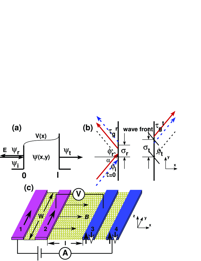
Figure 1: (color online) (a) Sectional and (b) top schematic views for a particle quantum tunneling through a potential barrier in graphene. The red solid and blue dashed lines respectively stand for the ballistic trajectories of the $A$ and $B$ components, which are located at $\pm 1/2k_{x}$, $\sigma_{r}\mp 1/2k_{x}$, and $\sigma_{t}\pm 1/2k_{x}$ for the incident, reflected, and transmitted beams, respectively. (c) Experimental setup for measuring the CGD by spin precession. Four ferromagnetic electrodes magnetized respectively along the $y$-, $y$-, $z(\bar{z})$-, and $z(\bar{z})$-axis are contacted to the graphene barrier, and a weak magnetic field is applied in the graphene plane along the $x$-axis. The contact induced potential contactresistance can be avoided by such four points probe huard2007transport and the intrinsic conductance through the barrier can be measured by $I_{14}/V_{23}|_{V_{23}\rightarrow 0}$. The length of the electrodes themselves are assumed to be small compared with $l$ so that the precession in them can be neglected.

Unlike in single-electron devices, the current in bulk graphene devices is contributed by numerous electrons or holes on half of the Fermi surface. This fact implies that a collective group delay (CGD) of all these particles rather than an individual group delay (IGD) of a single particle should be adopted to evaluate the tunneling speed in graphene. The CGD can be defined as the summation of mode ($n$)-dependent IGDs weighted with corresponding transmission probability ($T_{n}$), i.e., $\tau_{g}^{C}\equiv\Sigma_{n}T_{n}\tau_{g}^{(n)}$. In this work we theoretically investigate the CGD in graphene. Our motivation is two-fold. (i) CGD in graphene is not directly observable. Very recently, an approach using a Larmor clock dwelltime ; van has been suggested to measure the transmission times $\tau^{(p)}$ ($p=1,2$, $\tau^{(1)}=\tau_{g}^{C}/\Sigma_{n}T_{n}$) at the especial Fermi energy that aligns to the barrier charge neutrality point (or Dirac point) precession . However, the tunability of the Fermi energy is necessary in graphene devices; while the dynamics in graphene becomes totally different when the Fermi energy aligns to or diverges from the barrier Dirac point (i.e., pseudodiffusive precession for the former and ballistic miao2007phase ; du2008approaching for the latter case). So, how to measure the ballistic CGD at arbitrary Fermi energy is still a basic problem. To propose a feasible approach to measure the ballistic CGD at arbitrary Fermi energy is our first motivation. (ii) The ballistic transport in graphene is essentially two dimensional (2D). As a result, a lateral Goos-Hänchen (GH) shift GH occurs for the reflected or transmitted wave packet along the corresponding interface GHg1 ; GHg2 ; GHg3 ; giantGH (see Fig. 1b). As we will show, such GH shift makes an intrinsic contribution to the IGD. This fact has not been noticed in previous studies in graphene. It should be clarified no matter for the sake of itself or before we consider the measure problem of CGD. To obtain the complete expression of 2D IGD with the GH component contained is our second motivation.

In this work, through the analogy between ballistic electrons and photons, we obtain the complete expression of the 2D IGD and show that, the inherent GH component adds an asymmetric feature to the IGD’s energy dependence. By linking the 2D IGD to spin precession through the 2D dwell time, we further suggest that, for any Fermi energy comparable with the barrier height, the CGD and its GH component can be probed through conductance measurements in a spin precession experiment under weak magnetic fields.

II Inherent GH component in 2D IGD

To investigate the 2D IGD, let us consider the 2D quantum tunneling through a potential barrier in graphene (see, Fig. 1(a)(b)). The size of the graphene sample is set to be smaller than the electron mean free path ($\ell\sim$ 0.5-1$\mu$m miao2007phase ; du2008approaching ) and the phase-relaxation length ($L_{\phi}\sim$ 3-5$\mu$m miao2007phase ) to ensure the system stays in the ballistic coherent regime. A real potential occupies the region of $0<x<l$ and is translational invariant in the $y$-direction; it can be induced by a top gate due to the electric field effect electricfield . The Fermi energy is $E$ and can be controlled by a back gate electricfield . The sample width $W$ in the $y$-direction is several times of $l$ to ensure that the edge details are not important system .

An electron with a central incident angle of $\alpha\in(-\pi/2,\pi/2)$ at the Fermi surface incidents from the left side of the barrier. In the stationary state description, the spinor of electron envelope function $\Psi=(\psi_{A},\psi_{B})^{T}$ can be represented as a wave packet of a weighted superposition of plane wave spinors (each being a solution of Dirac’s equation) GHg1 ; giantGH . The appearing loci ($\sigma_{\xi}^{\eta}$) and moments ($\tau_{g}^{\xi\eta}$) for the $A$ and $B$ ($\eta=\pm$) component of the incident, reflection, and transmission ($\xi=i,r,t$) packet peaks (see, Fig. 1(b)) are determined by the following condition: the gradient of the total phase ($\phi_{T}^{\xi\eta}=\phi_{\xi}+k_{y}\sigma_{\xi}^{\eta}-E\tau_{g}^{\xi\eta}/\hbar$) in the wave vector ($\boldsymbol{k}=k_{x}\hat{x}+k_{y}\hat{y}$) space must vanish. Here, $r=|r|e^{i\phi_{r}}$ ($t=|t|e^{i\bar{\phi}_{t}}$) and $\phi_{r}$ ($\phi_{t}\equiv\bar{\phi}_{t}+k_{x}l$) are the reflection (transmission) coefficient and corresponding phase shift, respectively (see, Fig. 1(b)). This is similar to the optical case chiao but with the extra sublattice degree of freedom ($\eta$). Since $k_{x}=E\cos\alpha/\hbar v_{F}$ and $k_{y}=E\sin\alpha/\hbar v_{F}$, the above condition means two independent conditions $\partial\phi_{T}^{\xi\eta}/\partial E=0$ and $\partial\phi_{T}^{\xi\eta}/\partial k_{y}=0$. A comparison of the second conditions between the reflection (transmission) and incident beams gives the sublattice dependent lateral GH shift GHg1 ; giantGH : $\sigma^{\pm}_{r}=-(\partial\phi_{r}/\partial k_{y})_{E}\mp 1/k_{x}$ and $\sigma^{\pm}_{t}=-(\partial{\phi}_{t}/\partial k_{y})_{E}$ (see, Fig. 1(b)). A comparison of the first conditions gives the reflection and transmission 2D IGD,

$$\tau^{\xi}_{g}=\hbar\left[\frac{\partial(\phi_{\xi}+k_{y}\sigma_{\xi})}{\partial E}\right]_{\alpha}.$$ (1)

Here sublattice independent average values of GH shifts $\sigma_{\xi}=-(\partial\phi_{\xi}/\partial k_{y})_{E}$ have been used to evaluate the IGD for the electron spinor rather than its sublattice components. For asymmetric barriers, there is a difference between the reflection and transmission in both $\phi_{\xi}$ and $\sigma_{\xi}$, so a bidirectional 2D IGD can be defined as $\tau_{g}=\sum_{\xi}|\xi|^{2}\tau^{\xi}_{g}$.

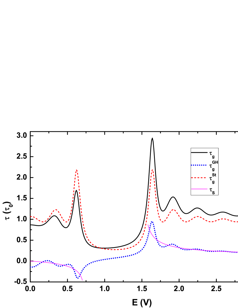
Figure 2: (color online) The 2D IGD, its scattering, and GH components (in units of the equal time $\tau_{0}\equiv l/v_{F}$) as a function of the Fermi energy at $\alpha=20^{\circ}$. The magenta thin solid curve stands for the time associated with the Snell shift, $\tau_{S}=\sigma_{S}\sin\alpha/v_{F}$. The parameters of the potential barrier (which are also used in Figs. 3-5) are $l/l_{0}=1$ and $V/E_{0}=3\pi$ with $l_{0}$ and $E_{0}\equiv\hbar v_{F}/l_{0}$ being a length unit and energy unit, respectively.

In the 1D case the bidirectional IGD has an expression of $\tau^{St}_{g}=\sum_{\xi}|\xi|^{2}\hbar d\phi_{\xi}/dE$, which stems solely from the phase shifts introduced by scattering at the interfaces particle . Comparing the two expressions, we can find that the differences come in two aspects between the 2D and 1D cases. Firstly, the differential in the 1D case becomes partial differential in the 2D one, i.e., $d/dE\rightarrow(\partial/\partial E)_{\alpha}$. Secondly, besides the scattering phase shifts in the 1D case, the GH shifts also contribute inherent phase shifts in the 2D case, i.e., $\phi_{\xi}\rightarrow\phi_{\xi}+k_{y}\sigma_{\xi}$.

To highlight the intrinsic contribution of the GH shifts, we rewrite the bidirectional 2D IGD as

$$\tau_{g}=\tau^{St}_{g}+\tau^{GH}_{g}.$$ (2)

The first component $\tau^{St}_{g}=\sum_{\xi}|\xi|^{2}\hbar(\partial\phi_{\xi}/\partial E)_{\alpha}$ comes from the scattering phase shifts at the interfaces, which is the same as the 1D case; while the second component $\tau^{GH}_{g}=\sum_{\xi}|{\xi}|^{2}\sigma_{\xi}\sin\alpha/v_{F}$ results from the GH shifts, which is totally absent in the 1D case. Note, we have used the relation $\hbar(\partial k_{y}/\partial E)_{\alpha}=\sin\alpha/v_{F}$ to get the GH component, since the GH shifts are not explicit functions of the energy. We would like to stress that, although the GH component displays a partial differential respective to $k_{y}$ at fixed $E$ (i.e., $\tau^{GH}_{g}=\sum_{\xi}|{\xi}|^{2}\sigma_{\xi}\sin\alpha/v_{F}$ and $\sigma_{\xi}=-(\partial\phi_{\xi}/\partial k_{y})_{E}$), this component essentially comes from the condition that the energy gradient of the GH phase shifts (i.e., $\partial/\partial E$) must vanish. We can understand the GH component as following. At time $\hbar(\partial{\phi}_{t}/\partial E)_{\alpha}$, the wave front of the transmitted beam reaches $(l,0)$ and then propagates freely with a velocity of $v_{F}$ to the final position $(l,\sigma_{t})$ (see, Fig. 1(b)). This step will cost a duration of $\sigma_{t}\sin\alpha/v_{F}$ since the wave front is perpendicular to the propagation direction. This picture also holds for the reflected beam. A weighted average of the transmission and reflection gives $\tau^{GH}_{g}$.

Figure 2 shows clearly the contribution of the GH component to the 2D IGD. One can see that $\tau_{g}^{St}$ is symmetric about the center ($E/V=\cos^{-2}\alpha$) of the transmission gap (TG) due to the symmetry of $\phi_{\xi}$ about it. On the contrary, $\tau_{g}^{GH}$ stemming from the quantum GH shifts is asymmetric about the TG’s center. The quantum GH shift displays the same trend as the classical shift predicted by the Snell’s law ($\sigma_{S}=l\tan\beta$ with $\beta=\sin^{-1}(\hbar v_{F}k_{y}/(E-V))$ being the refracted angle). The latter is obviously asymmetric as it is negative (positive) in the low (high) energy range (see Fig. 2). In total, the GH component not only quantitatively contributes a part of order of $\sigma_{S}\sin\alpha/v_{F}$ to the 2D IGD, but also qualitatively results in the remarkable asymmetric feature in the energy dependence of the 2D IGD.

III Measuring the CGD by spin precession-induced conductance difference

Having obtained the complete expression for the IGD, we now seek physical observable for the CGD at arbitrary Fermi energy. The Larmor precession of the electron spin in a magnetic field provides a clock for studying the electron dynamics Larmor-clock ; dwelltime ; precession . Here, we consider a configuration where the magnetic field is applied in the graphene plane along the $x$-axis (see, Fig. 1(c)). In such a configuration, the dynamical perturbation by the Lorentz force is avoided, and the only effect of the magnetic field is to cause spin precession round the $x$-axis. For electrons with spins initially directing the $y$-axis, a duration of this precession leads to different transmission probabilities in the $z$ and $\bar{z}$ directions. We calculate the spin-dependent transmission probability ($T_{z(\bar{z})y}=|t_{z(\bar{z})y}|^{2}$) in a pseudospin-spin direct product space (a similar method is used in Ref. precession ), where $T_{z(\bar{z})y}$ denotes the transmission probability for an electron incident from electrode 2 (with $y$-directed spin) and transmitted to electrode 3 (with $z$ or $\bar{z}$-directed spin) (see, Fig. 1(c)). An explicit equality between the spin polarization in transmission probabilities $P\equiv(T_{zy}-T_{\bar{z}y})/(T_{zy}+T_{\bar{z}y})$ and the dwell time ($\tau_{d}=\int_{0}^{l}|\psi(x)|^{2}dx/(v_{F}\cos\alpha)$) is found in the weak-field limit:

$$\tau_{d}=(P/\omega_{B})|_{\mathcal{B}\rightarrow 0},$$ (3)

where, $\omega_{B}=g\mu_{B}B$ is the Larmor frequency, $g$ is the gyromagnetic factor in graphene, $\mu_{B}$ is the Bohr magneton, and $B$ is the magnetic field with a reduced strength $\mathcal{B}\equiv\hbar\omega_{B}/2E_{0}$. This equality is clearly demonstrated in Fig. 3. Note, this equality is restricted in symmetric structures sym . Under such restriction Eq. (3) holds for arbitrary incident energies and angles and can be interpreted physically in following. Rewriting the equality as $\omega_{B}\tau_{d}=P$ and multiplying both sides by $\hbar/2$, the right hand side gives the expectation value of $S_{z}$ of the transmitted electrons. Such expectation value is determined by the product of the spin precession frequencey (i.e., the Larmor frequency) and the time the precession persists (i.e., the dwell time). This is just what the left hand side expresses. It is noted that Eq. (3) also holds in systems with parabolic dispersion relations and scale envelope functions dwelltime .

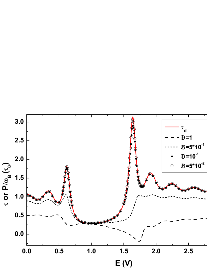
Figure 3: (color online) The dwell time and $P/\omega_{B}$ at various $\mathcal{B}$ as a function of the Fermi energy at $\alpha=20^{\circ}$.

To obtain the summation of the dwell time on half of the Fermi surface, we multiply Eq. (3) by $(T_{zy}+T_{\bar{z}y})/2$ (which tends to $T$ when $\mathcal{B}\rightarrow 0$). Then the right hand side of Eq. (3) can be further related to an experimental observable, the conductance ($G$). This is because the conductance is defined as $G(E)=G_{0}\sum_{n}T_{n}$, where $G_{0}=2e^{2}/h$ is the quantum conductance considering the twofold valley degeneracy. Thus, Eq. (3) can be rewritten as

$$\sum_{n}\tau_{d}^{(n)}T_{n}=\frac{G_{zy}(E)-G_{\bar{z}y}(E)}{2\omega_{B}G_{0}}|_{\mathcal{B}\rightarrow 0},$$ (4)

where $G_{z(\bar{z})y}$ can be probed by $I_{14}/V_{23}|_{V_{23}\rightarrow 0}$ in the proposed experimental setup (see, Fig. 1(c)).

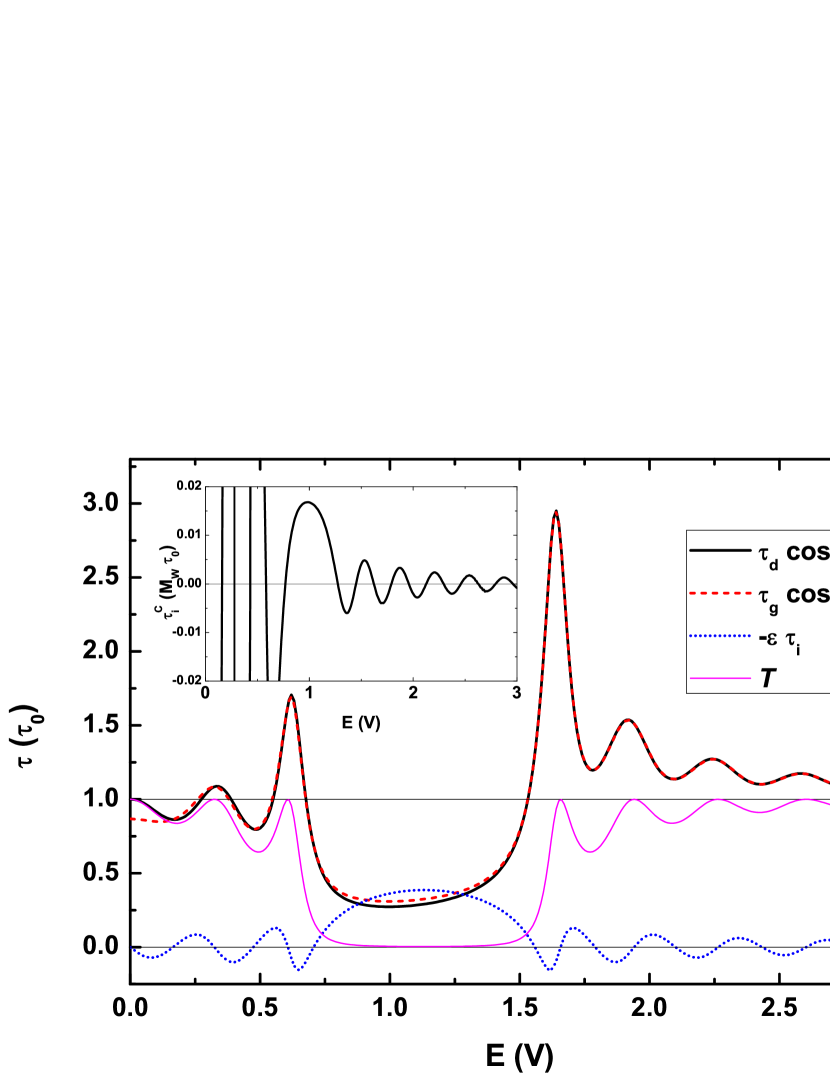
Figure 4: (color online) The reduced IGD, dwell time, self-interference delay, and transmission probability as a function of the Fermi energy at $\alpha=20^{\circ}$. Insert: the collective self-interference delay versus the Fermi energy.

We now try to link the CGD to the above conductance difference by the relation between the 2D IGD and the 2D dwell time. This relation can be obtained by making a variation of the time-independent Dirac equation at the barrier boundary with respect to the two individual variational parameters, ($k_{x}$, $k_{y}$) or equivalently ($E$, $\alpha$). The 2D feature of the tunneling process and the spinor nature of envelope functions should be taken into account in the variation, for which the detailed derivations can be found in the Appendix. We make the variation with respect to $E$ and $\sin\alpha$, since the variation results about them can be expediently related to $\tau_{g}^{St}$ (see, Eqs. (9)-(13) in the Appendix) and $\tau_{g}^{GH}$ (see, Eqs. (14)-(15) in the Appendix), respectively. The concise result for a rectangular barrier reads

$$\tau_{d}=\tau_{g}+\tau_{i},$$ (5)

where $\tau_{i}=\hbar[\textmd{Re}(r)\cos\alpha+\textmd{Im}(r)\sin\alpha]\sin\alpha/(E\cos^{2}\alpha)$ is a self-interference delay (see, Eq. (13) in the Appendix) stemming from the interference of the incident and reflection envelope functions in front of the barrier review ; interference . The correctness of this relation can be verified by numerically calculating and comparing the explicit expressions of $\tau_{d}$, $\tau_{g}$, and $\tau_{i}$.

Fig. 4 shows the 2D IGD, dwell time, and self-interference delay in reduced form as a function of the Fermi energy at a fixed incident angle, where $\epsilon\equiv E/E_{0}$ is the reduction factor. One can see that the reduced self-interference delay ($-\epsilon\tau_{i}$) is symmetric about the TG’s center; it achieves the maximum at the TG’s center and oscillates around zero outside the TG. The self-interference delay itself is important only in the low energy range (diverging as $E^{-1}$ when $E\rightarrow 0$). It disappears at (anti)resonant tunneling since there is no interference in front of the barrier. Accordingly, the IGD almost coincides with the dwell time except within the low energy range or around the TG’s center.

The collective self-interference delay ($\tau_{i}^{C}$) can be calculated by using $\sum_{n}T_{n}(E)\tau_{i}^{(n)}(E)=M\int_{-\pi/2}^{\pi/2}\tau_{i}(E,\alpha)T(E,\alpha)d(\sin\alpha)$, where $M=|E|W/hv_{F}=(|E|/E_{0})(W/2\pi l_{0})\equiv M_{E}M_{W}$ is the number of the transverse modes (which should be rather big). As can be seen in the insert of Fig. 4, $\tau_{i}^{C}$ oscillates with $E$ with the amplitude disappearing exponentially at a relatively high Fermi energy. Therefore, Eqs. (4) and (5) imply that, for arbitrary Fermi energies comparable with $V$, the CGD can be directly measured by the spin-precession induced conductance difference under weak fields

$$\tau_{g}^{C}(E)\approx\frac{G_{zy}-G_{\bar{z}y}}{2\omega_{B}G_{0}}|_{\mathcal{B}\rightarrow 0}.$$ (6)

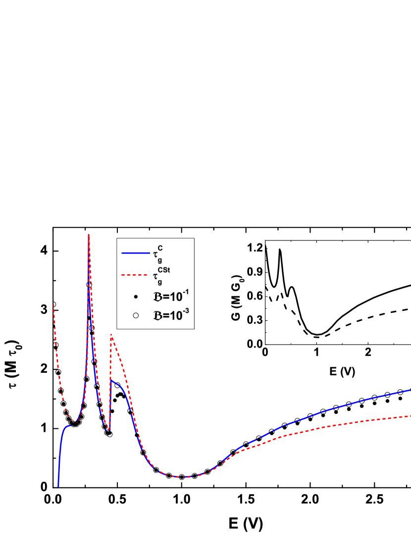
Figure 5: (color online) The CGD, its scattering component, and the $\mathcal{B}$-dependent conductance difference (i.e., the right hand of Eq. (6)) as a function of the Fermi energy. Insert: $G_{zy}$ (solid) and $G_{\bar{z}y}$ (dashed) could be directly measured in the experiment for $\mathcal{B}=10^{-1}$.

Fig. 5 shows the CGD, its scattering component, and the magnetic field dependent conductance differences as a function of the Fermi energy. To clearly show the oscillation details in the low energy range, all these qualities are plotted for a single mode (i.e., divided by $M$). As is seen, the spin-precession induced conductance difference can be obtained by measuring $G_{zy}$ and $G_{\bar{z}y}$ separately (see insert in Fig. 5) and it increases for weaker $\mathcal{B}$ (see Fig. 5). At $\mathcal{B}=10^{-3}$, it is already a rather good measurement of the CGD for $E>0.2V$. Thus, we provide an electrostatic approach to measure the CGD in graphene, which is feasible for almost arbitrary Fermi energy. This approach looks interesting when we notice that the CGD describes a dynamic process while the conductance is static.

In Fig. 5, it is also noted that, due to the GH shifts with different signs, the scattering component is always larger (smaller) than the expected value of the CGD when $E<V$ ($E>V$). Then, a comparison between the experimentally observed value of the conductance difference (the right hand side of Eq. (6)) and the theoretical prediction of the CGD (the left hand side of Eq. (6)) at Fermi energies away from the barrier Dirac point can be utilized to probe the inherent GH component of the CGD (or equivalently the intrinsic effect of the GH shifts on the CGD) in graphene.

IV Conclusions and Remarks

In summary, we have obtained the complete expression of the 2D IGD in graphene with the intrinsic contribution of the GH shifts being contained. Moreover, we have proposed an approach to probe the ballistic CGD and its inherent GH component by conductance measurements in a weak-field spin precession experiment. This approach is feasible for almost arbitrary Fermi energy. We have also indicated that, it is a generally nonzero self-interference delay that relates the 2D IGD and dwell time in graphene. The inherent GH component of the 2D IGD should also present in other 2D ballistic coherent electronic systems, since the derivations of it do not depend on the specific electronic excitation of graphene. The feasibility of the proposed approach to measure CGD in these systems is an interesting question.

V Acknowledgement

YS benefited from discussions with Prof. C. W. J. Beenakker and HCW was grateful to the SFI Short Term Travel fellowship support during his stay at PKU. This project was supported by the 973 Program of China (2011CB606405).

Appendix A Derivation for the relation between 2D IGD and dwell time in graphene

Let us begin with the single-particle Dirac equation that governs the low-energy excitation in graphene. In the barrier region it reads as $[v_{F}\boldsymbol{\sigma}\cdot\mathbf{p}+V(x)]\boldsymbol{\Psi}(x,y)=E\boldsymbol{\Psi}(x,y),$ where the pseudospin matrix $\boldsymbol{\sigma}$ has components given by Pauli’s matrices and $\mathbf{p}=(p_{x},p_{y})$ is the momentum operator. The eigenstates $\boldsymbol{\Psi}(x,y)$ are two-component spinors with each component being the envelope function at sublattice site $A/B$ of the graphene sheet. Due to the translational invariance along the $y$-axis, the envelope function can be separated as $\boldsymbol{\Psi}=[\psi_{A}(x),\,\psi_{B}(x)]^{T}e^{ik_{y}y}$ with $k_{y}=E\sin\alpha/\hbar v_{F}$. The $A$ and $B$ components along the $x$-direction are related by a pair of coupling first-order equations

$$\frac{\partial}{\partial x}\psi_{A,B}=\pm k_{y}\psi_{A,B}-\frac{E-V}{i\hbar v_{F}}\psi_{B,A},$$ (7)

which imply a decoupled second-order equation for both the $A$- and $B$-components

$$\left[\frac{\partial^{2}}{\partial x^{2}}+\frac{(E-V){}^{2}-E^{2}\sin^{2}\alpha}{(\hbar v_{F})^{2}}\right]\psi_{A,B}=0.$$ (8)

We carry out the energy-variational form and conjugate form of Eq. (8) and upon integration over the length of the barrier we get

$$\begin{split}&\left.\left(\frac{\partial\psi_{A,B}}{\partial E}\frac{\partial\psi_{A,B}^{*}}{\partial x}-\psi_{A,B}^{*}\frac{\partial^{2}\psi_{A,B}}{\partial E\partial x}\right)_{\alpha}\right|_{x=0}^{x=l}\\ &=\int_{0}^{l}\frac{2E\cos^{2}\alpha-2V(x)}{(\hbar v_{F})^{2}}|\psi_{A,B}|^{2}dx.\end{split}$$ (9)

It is found that when is evaluated by the envelope function outside (inside) the barrier, the left (right) part can be related to $\tau_{g}^{St}$ ($\tau_{d}$). However, we should note that Eq. (9) is only valid inside the barrier as the spatial derivative of $\psi_{A,B}$ are not continuous on the potential boundary. To overcome this dilemma, we express $\partial\psi_{A,B}/\partial x$ inside the barrier by Eq. (7) and their conjugate form. Since $\psi_{A,B}$ themselves are continuous, envelope functions inside the barrier can be replaced by the corresponding ones outside the barrier. Then the left part of Eq. (9) can be evaluated. For the $A$-component it reads as

$$J+K+\cos\alpha(-ir+ir^{*})/\hbar v_{F},$$ (10a)

and for the $$B$$-component, the result becomes

$$J+K+\cos\alpha(ie^{-i2\alpha}r-ie^{i2\alpha}r^{*})/\hbar v_{F},$$ (10b)

where $J=\frac{iE}{\hbar v_{F}}\{[B(0)-A(0)]|r|^{2}\phi_{r}^{\prime}+[B(l)-A(l)]|t|^{2}\phi_{t}^{\prime}\}$ and $K=\frac{E}{\hbar v_{F}}\{[B(0)-A(0)]|r||r|^{\prime}+[B(l)-A(l)]|t||t|^{\prime}\}.$ Here the relation of lossless barriers $|t|^{2}+|r|^{2}=1$ has been used and the notations are adopted as $O^{\prime}\equiv(\partial O/\partial E)_{\alpha}$, $A(x)=\sin\alpha+i\lambda(x)e^{i\alpha}$, $B(x)=\sin\alpha-i\lambda(x)e^{-i\alpha}$, and $\lambda(x)=1-V(x)/E$, a ratio of the kinetic energy inside and outside the barrier.

Since $\psi^{*}\psi=\psi_{A}^{*}\psi_{A}+\psi_{B}^{*}\psi_{B}$, the relation for each spinor component should be added to get the relation for the spinor, which at last reads

$$\begin{split}&\frac{\int_{0}^{l}[\lambda(x)-\sin^{2}\alpha]|\psi(x)|^{2}dx}{v_{F}\cos\alpha}\\ =&\lambda(0)|r|^{2}\hbar\phi_{r}^{\prime}+\lambda(l)|t|^{2}\hbar\phi_{t}^{\prime}-i\lambda(0)\hbar|r||r|^{\prime}-i\lambda(l)\hbar|t||t|^{\prime}\\ &+\hbar\frac{[\textmd{Re}(r)\cos\alpha+\textmd{Im}(r)\sin\alpha]\sin\alpha}{k}\frac{\partial k}{\partial E},\end{split}$$ (11)

where $\textmd{Re}(r)$ ($\textmd{Im}(r)$) is the real (imaginary) part of $r$. We can see that, this equation is a general result that relates the integral of the weighted probability density inside the barrier (left part) and the weighted energy-variational behavior outside the barrier (right part). It is noted that, the factor $\lambda(x)$ has a critical role in the relation.

To clearly relate the general result Eq. (11) with both $\tau_{d}$ and $\tau_{g}^{St}$, we consider a restricted condition that $\lambda(x)$ is a constant under the barrier (i.e., a rectangular barrier). Note this condition is not necessary for the common semiconductors case particle , a reflection of the spinor nature of graphene. Under such condition, the third and fourth terms on the right hand side of Eq. (11) disappear due to the lossless condition of the barrier $|t||t|^{\prime}+|r||r|^{\prime}=0$, and Eq. (11) can be rewritten in terms of $\tau_{d}$ and $\tau_{g}^{St}$, i.e., as a sub-relation

$$\tau_{d}(\lambda-\sin^{2}\alpha)=\tau^{St}_{g}\lambda+\tau_{i}\cos^{2}\alpha,$$ (12)

where a self-interference delay is found from the last term of Eq. (11),

$$\tau_{i}=\frac{\hbar[\textmd{Re}(r)\cos\alpha+\textmd{Im}(r)\sin\alpha]\sin\alpha}{E\cos^{2}\alpha}.$$ (13)

Graphene is two dimensional, which means there are two independent variation parameters, $k_{x}$ and $k_{y}$ or $E$ and $\sin\alpha$. We have made the variation about $E$, the variation of Eq. (8) about $\sin\alpha$ reads

$$\begin{split}&\left.\left(\frac{\partial\psi_{A,B}}{\partial\sin\alpha}\frac{\partial\psi_{A,B}^{*}}{\partial x}-\psi_{A,B}^{*}\frac{\partial^{2}\psi_{A,B}}{\partial\sin\alpha\partial x}\right)_{E}\right|_{x=0}^{x=l}\\ &=\int_{0}^{l}\frac{-2E^{2}\sin\alpha}{(\hbar v_{F})^{2}}|\psi_{A,B}|^{2}dx.\end{split}$$ (14)

Following a similar way as above, we straightforwardly obtain the sub-relation between $\tau_{d}$ and $\tau_{g}^{GH}$ under the same restricted condition of a constant $\lambda$. The sub-relation reads

$$\tau_{d}\sin^{2}\alpha=\tau^{GH}_{g}\lambda+\tau_{i}(\lambda-\cos^{2}\alpha).$$ (15)

Making a simple addition of the two sub-relations in Eqs. (12) and (15) and taking into account $\tau_{g}=\tau^{St}_{g}+\tau^{GH}_{g}$ (see, Eq. (2) in the main body), we finally get

$$\tau_{d}=\tau_{g}+\tau_{i}.$$ (16)

The correctness of this relation and the sub-relations can be verified by numerically calculating and comparing the explicit expressions of the five times. It may be valuable to indicate that, many previous works hartman12 ; dwell ; gap have also concerned such relation and they all have achieved a same conclusion that $\tau_{g}=\tau_{d}$ (actually they mean $\tau_{g}^{St}=\tau_{d}$ since $\tau_{g}^{GH}$ is not included in their discussions). The results obtained here clearly indicate that, it is a self-interference delay that relates the group delay and dwell time in graphene, similar to the common semiconductor case particle .

For the normal incident or 1D tunneling case ($\alpha=0$), $\tau_{i}$ vanishes (see the factor $\sin\alpha$ in Eq. (13)), since no reflected portion thus no interference happens in front of the barrier due to the Klein tunneling klein . The relation and subrelations revealed in Eqs. (16), (12), and (15) and the expression for the self-interference delay Eq. (13) also hold for the tunneling of massless Dirac particles in topological surface states TI , where the real electron spin rather than the sublattice structure in graphene provides the Dirac structure.

References

- (1) E. H. Hauge and J. A. Støvneng, Rev. Mod. Phys. 61, 917 (1989).
- (2) R. Landauer and Th. Martin, Rev. Mod. Phys. 66, 217 (1994).
- (3) E. P. Wigner, Phys. Rev. 98, 145 (1955).
- (4) F. T. Smith, Phys. Rev. 118, 349 (1960).
- (5) M. Büttiker, Phys. Rev. B 27, 6178 (1983).
- (6) H. Mizuta and T. Tanoue, The Physics and Applications of Resonant Tunneling Diodes (Cambridge University Press, Cambridge, 1995).
- (7) A. E. Bernardini, Ann. Phys. 324, 1303 (2009).
- (8) R. A. Sepkhanov, M. V. Medvedyeva, and C. W. J. Beenakker, Phys. Rev. B 80, 245433 (2009).
- (9) Z. Wu, K. Chang, J. T. Liu, X. J. Li, and K. S. Chan, J. Appl. Phys. 105, 043702 (2009); D. Dragoman and M. Dragoman, ibid. 107, 054306 (2010).
- (10) Y. Gong and Y. Guo, J. Appl. Phys. 106, 064317 (2009); X. G. Xu and J. C. Cao, Physica B 407, 281 (2012).
- (11) M. Esmailpour, A. Esmailpour, R. Asgari, M. Elahi, and M. R. Rahimi Tabar, Solid State Commun. 150, 655 (2010).
- (12) J. T. Liu, F. H. Su, H. Wang, and X. H. Deng, New J. Phys. 14, 013012 (2012).
- (13) F. Sattari and E. Faizabadi, AIP Adv. 2, 012123 (2012); E. Faizabadi and F. Sattari, J. Appl. Phys. 111, 093724 (2012).
- (14) N. Tombros, C. Jozsa, M. Popinciuc, H. T. Jonkman, and B. J. van Wees, Nature (London) 448, 571 (2007).
- (15) F. Miao, S. Wijeratne, Y. Zhang, et al., Science, 317, 1530 (2007).
- (16) X. Du, I. Skachko, A. Barker, et al., Nature Nano. 3, 491 (2008).
- (17) This shift is named after the physicists who first observed it. See, F. Goos and H. Hänchen, Ann. Phys. (Leipzig) 436, 333 (1947).
- (18) C. W. J. Beenakker, R. A. Sepkhanov, A. R. Akhmerov, and J. Tworzydło, Phys. Rev. Lett. 102, 146804 (2009).
- (19) X. Chen, J. W. Tao, and Y. Ban, Euro. Phys. J. B 79, 203 (2011); M. Sharma and S. Ghosh, J. Phys.: Condens. Matter 23, 055501 (2011).
- (20) Z. Wu, F. Zhai, F. M. Peeters, H. Q. Xu, and K. Chang, Phys. Rev. Lett. 106, 176802 (2011); F. Zhai, Y. Ma, and K. Chang, New J. Phys. 13, 083029 (2011).
- (21) Y. Song, H. C. Wu, and Y. Guo, Appl. Phys. Lett. 100, 253116 (2012).
- (22) Y. Wu, V. Perebeinos, Y. M. Lin, T. Low, F. Xia, and P. Avouris, Nano Lett. 12, 1417 (2012).
- (23) B. Huard, J. Sulpizio, N. Stander, et al., Phys. Rev. Lett. 98, 236803 (2007).
- (24) K. S. Novoselov, A. K. Geim, S. V. Morozov, D. Jiang, Y. Zhang, S. V. Dubonos, I. V. Grigorieva, and A. A. Firsov, Science 306, 666 (2004).
- (25) J. Tworzydło, B. Trauzettel, M. Titov, A. Rycerz, and C. W. J. Beenakker, Phys. Rev. Lett. 96, 246802 (2006).
- (26) A. M. Steinberg and R. Y. Chiao, Phys. Rev. A 49, 3283 (1994); C. F. Li, ibid. 65, 066101 (2002).
- (27) H. G. Winful, Phys. Rev. Lett. 91, 260401 (2003).
- (28) A. I. Baz’, Sov. J. Nucl. Phys. 4, 182 (1967); ibid. 5, 161 (1967); V. F. Rybachenko, ibid. 5, 635 (1967).
- (29) C. R. Leavens and G. C. Aers, Solid State Commun. 63, 1101 (1987).
- (30) E. H. Hauge, J. P. Falck and T. A. Fjeldly, Phys. Rev. B 36, 4203 (1987).
- (31) M. I. Katsnelson, K. S. Novoselov, and A. K. Geim, Nature Phys. 2, 620 (2006).
- (32) X. L. Qi and S. C. Zhang, Rev. Mod. Phys. 83, 1057 (2011).