Distributed Low-rank Subspace Segmentation

Abstract

Vision problems ranging from image clustering to motion segmentation to semi-supervised learning can naturally be framed as subspace segmentation problems, in which one aims to recover multiple low-dimensional subspaces from noisy and corrupted input data. Low-Rank Representation (LRR), a convex formulation of the subspace segmentation problem, is provably and empirically accurate on small problems but does not scale to the massive sizes of modern vision datasets. Moreover, past work aimed at scaling up low-rank matrix factorization is not applicable to LRR given its non-decomposable constraints. In this work, we propose a novel divide-and-conquer algorithm for large-scale subspace segmentation that can cope with LRR’s non-decomposable constraints and maintains LRR’s strong recovery guarantees. This has immediate implications for the scalability of subspace segmentation, which we demonstrate on a benchmark face recognition dataset and in simulations. We then introduce novel applications of LRR-based subspace segmentation to large-scale semi-supervised learning for multimedia event detection, concept detection, and image tagging. In each case, we obtain state-of-the-art results and order-of-magnitude speed ups.

^a Department of Electrical Engineering and Computer Science, UC Berkeley
^b Department of Statistics, Stanford
^c Department of Electrical Engineering, Columbia
^d Department of Statistics, UC Berkeley

1 Introduction

Visual data, though innately high dimensional, often reside in or lie close to a union of low-dimensional subspaces. These subspaces might reflect physical constraints on the objects comprising images and video (e.g., faces under varying illumination [2] or trajectories of rigid objects [24]) or naturally occurring variations in production (e.g., digits hand-written by different individuals [12]). Subspace segmentation techniques model these classes of data by recovering bases for the multiple underlying subspaces [10, 7]. Applications include image clustering [7], segmentation of images, video, and motion [30, 6, 26], and affinity graph construction for semi-supervised learning [32].

One promising, convex formulation of the subspace segmentation problem is the low-rank representation (LRR) program of Liu et al. [17, 18]:

$$(\hat{{\mathbf{Z}}},\hat{{\mathbf{S}}})=\mathop{\mathrm{missing}}{argmin}_{{\mathbf{Z}},{\mathbf{S}}}\quad{\|{{\mathbf{Z}}}\|}_{*}+\lambda{\|{{\mathbf{S}}}\|}_{2,1}$$ (1)

$$\text{subject\, to}\quad{\mathbf{M}}={\mathbf{M}}{\mathbf{Z}}+{\mathbf{S}}\,.$$

Here, ${\mathbf{M}}$ is an input matrix of datapoints drawn from multiple subspaces, ${\|{\cdot}\|}_{*}$ is the nuclear norm, ${\|{\cdot}\|}_{2,1}$ is the sum of the column $\ell_{2}$ norms, and $\lambda$ is a parameter that trades off between these penalties. LRR segments the columns of ${\mathbf{M}}$ into subspaces using the solution $\hat{{\mathbf{Z}}}$, and, along with its extensions (e.g., LatLRR [19] and NNLRS [32]), admits strong guarantees of correctness and strong empirical performance in clustering and graph construction applications. However, the standard algorithms for solving Eq. (1) are unsuitable for large-scale problems, due to their sequential nature and their reliance on the repeated computation of costly truncated SVDs.

Much of the computational burden in solving LRR stems from the nuclear norm penalty, which is known to encourage low-rank solutions, so one might hope to leverage the large body of past work on parallel and distributed matrix factorization [11, 23, 8, 31, 21] to improve the scalability of LRR. Unfortunately, these techniques are tailored to optimization problems with losses and constraints that decouple across the entries of the input matrix. This decoupling requirement is violated in the LRR problem due to the ${\mathbf{M}}={\mathbf{M}}{\mathbf{Z}}+{\mathbf{S}}$ constraint of Eq. (1), and this non-decomposable constraint introduces new algorithmic and analytic challenges that do not arise in decomposable matrix factorization problems.

To address these challenges, we develop, analyze, and evaluate a provably accurate divide-and-conquer approach to large-scale subspace segmentation that specifically accounts for the non-decomposable structure of the LRR problem. Our contributions are three-fold:

Algorithm: We introduce a parallel, divide-and-conquer approximation algorithm for LRR that is suitable for large-scale subspace segmentation problems. Scalability is achieved by dividing the original LRR problem into computationally tractable and communication-free subproblems, solving the subproblems in parallel, and combining the results using a technique from randomized matrix approximation. Our algorithm, which we call DFC-LRR, is based on the principles of the Divide-Factor-Combine (DFC) framework [21] for decomposable matrix factorization but can cope with the non-decomposable constraints of LRR.

Analysis: We characterize the segmentation behavior of our new algorithm, showing that DFC-LRR maintains the segmentation guarantees of the original LRR algorithm with high probability, even while enjoying substantial speed-ups over its namesake. Our new analysis features a significant broadening of the original LRR theory to treat the richer class of LRR-type subproblems that arise in DFC-LRR. Moreover, since our ultimate goal is subspace segmentation and not matrix recovery, our theory guarantees correctness under a more substantial reduction of problem complexity than the work of [21] (see Sec. 3.2 for more details).

Applications: We first present results on face clustering and synthetic subspace segmentation to demonstrate that DFC-LRR achieves accuracy comparable to LRR in a fraction of the time. We then propose and validate a novel application of the LRR methodology to large-scale graph-based semi-supervised learning. While LRR has been used to construct affinity graphs for semi-supervised learning in the past [4, 32], prior attempts have failed to scale to the sizes of real-world datasets. Leveraging the favorable computational properties of DFC-LRR, we propose a scalable strategy for constructing such subspace affinity graphs. We apply our methodology to a variety of computer vision tasks – multimedia event detection, concept detection, and image tagging – demonstrating an order of magnitude improvement in speed and accuracy that exceeds the state of the art.

The remainder of the paper is organized as follows. In Section 2 we first review the low-rank representation approach to subspace segmentation and then introduce our novel DFC-LRR algorithm. Next, we present our theoretical analysis of DFC-LRR in Section 3. Section 4 highlights the accuracy and efficiency of DFC-LRR on a variety of computer vision tasks. We present subspace segmentation results on simulated and real-world data in Section 4.1. In Section 4.2 we present our novel application of DFC-LRR to graph-based semi-supervised learning problems, and we conclude in Section 5.

Notation Given a matrix ${\mathbf{M}}\in\mathbb{R}^{m\times n}$, we define ${\mathbf{U}}_{M}{\mathbf{\Sigma}}_{M}{\mathbf{V}}_{M}^{\top}$ as the compact singular value decomposition (SVD) of ${\mathbf{M}}$, where $\mathrm{rank}({{\mathbf{M}}})=r$, ${\mathbf{\Sigma}}_{M}$ is a diagonal matrix of the $r$ non-zero singular values and ${\mathbf{U}}_{M}\in\mathbb{R}^{m\times r}$ and ${\mathbf{V}}_{M}\in\mathbb{R}^{n\times r}$ are the associated left and right singular vectors of ${\mathbf{M}}$. We denote the orthogonal projection onto the column space of ${\mathbf{M}}$ as ${\mathbf{P}}_{M}$.

2 Divide-and-Conquer Segmentation

In this section, we review the LRR approach to subspace segmentation and present our novel algorithm, DFC-LRR.

2.1 Subspace Segmentation via LRR

In the robust subspace segmentation problem, we observe a matrix ${\mathbf{M}}={\mathbf{L}}_{0}+{\mathbf{S}}_{0}\in\mathbb{R}^{m\times n}$, where the columns of ${\mathbf{L}}_{0}$ are datapoints drawn from multiple independent subspaces, and ${\mathbf{S}}_{0}$ is a column-sparse outlier matrix. Our goal is to identify the subspace associated with each column of ${\mathbf{L}}_{0}$, despite the potentially gross corruption introduced by ${\mathbf{S}}_{0}$. An important observation for this task is that the projection matrix ${\mathbf{V}}_{L_{0}}{\mathbf{V}}_{L_{0}}^{\top}$ for the row space of ${\mathbf{L}}_{0}$, sometimes termed the shape iteration matrix, is block diagonal whenever the columns of ${\mathbf{L}}_{0}$ lie in multiple independent subspaces [10]. Hence, we can achieve accurate segmentation by first recovering the row space of ${\mathbf{L}}_{0}$.

The LRR approach of [17] seeks to recover the row space of ${\mathbf{L}}_{0}$ by solving the convex optimization problem presented in Eq. (1). Importantly, the LRR solution comes with a guarantee of correctness: the column space of $\hat{{\mathbf{Z}}}$ is exactly equal to the row space of ${\mathbf{L}}_{0}$ whenever certain technical conditions are met [18] (see Sec. 3 for more details).

Moreover, as we will show in this work, LRR is also well-suited to the construction of affinity graphs for semi-supervised learning. In this setting, the goal is to define an affinity graph in which nodes correspond to data points and edge weights exist between nodes drawn from the same subspace. LRR can thus be used to recover the block-sparse structure of the graph’s affinity matrix, and these affinities can be used for semi-supervised label propagation.

2.2 Divide-Factor-Combine LRR (DFC-LRR)

We now present our scalable divide-and-conquer algorithm, called DFC-LRR, for LRR-based subspace segmentation. DFC-LRR extends the principles of the DFC framework of [21] to a new non-decomposable problem. The DFC-LRR algorithm is summarized in Algorithm 1, and we next describe each step in further detail.

D step - Divide input matrix into submatrices: DFC-LRR randomly partitions the columns of ${\mathbf{M}}$ into $t$ $l$-column submatrices, $\{{\mathbf{C}}_{1},\ldots,{\mathbf{C}}_{t}\}$. For simplicity, we assume that $t$ divides $n$ evenly.

F step - Factor submatrices in parallel: DFC-LRR solves $t$ subproblems in parallel. The $i$th LRR subproblem is of the form

$$\min_{{\mathbf{Z}}_{i},{\mathbf{S}}_{i}}\quad{\|{{\mathbf{Z}}_{i}}\|}_{*}+\lambda{\|{{\mathbf{S}}_{i}}\|}_{2,1}$$ (2)

$$\text{subject\, to}\quad{\mathbf{C}}_{i}={\mathbf{M}}{\mathbf{Z}}_{i}+{\mathbf{S}}_{i}\,,$$

where the input matrix ${\mathbf{M}}$ is used as a dictionary but only a subset of columns is used as the observations. A typical LRR algorithm can be easily modified to solve Eq. (2) and will return a low-rank estimate $\hat{\mathbf{Z}}_{i}$ in factored form.

C step - Combine submatrix estimates: DFC-LRR generates a final approximation ${\hat{{\mathbf{Z}}}^{proj}}$ to the low-rank LRR solution $\hat{{\mathbf{Z}}}$ by projecting $[\hat{\mathbf{Z}}_{1},\ldots,\hat{\mathbf{Z}}_{t}]$ onto the column space of $\hat{\mathbf{Z}}_{1}$. This column projection technique is commonly used to produce randomized low-rank matrix factorizations [15] and was also employed by the DFC-Proj algorithm of [21].

Runtime: As noted in [21], many state-of-the-art solvers for nuclear-norm regularized problems like Eq. (1) have $\Omega(mnk_{M})$ per-iteration time complexity due to the rank-$k_{M}$ truncated SVD required on each iteration. DFC-LRR reduces this per-iteration complexity significantly and requires just O$(mlk_{C_{i}})$ time for the $i$th subproblem. Performing the subsequent column projection step is relatively cheap computationally, since an LRR solver can return its solution in factored form. Indeed, if we define $k^{\prime}\triangleq\max_{i}k_{C_{i}}$, then the column projection step of DFC-LRR requires only O$(mk^{\prime 2}+lk^{\prime 2})$ time.

Algorithm 1 DFC-LRR

  Input: ${\mathbf{M}}$, $t$

  $\{{\mathbf{C}}_{i}\}_{1\leq i\leq t}$ = SampleCols(${\mathbf{M}}$, $t)$ do in parallel

        $\hat{{\mathbf{Z}}}_{1}$ = LRR$({\mathbf{C}}_{1},{\mathbf{M}})$

                    ⋮

        $\hat{{\mathbf{Z}}}_{t}$ = LRR$({\mathbf{C}}_{t},{\mathbf{M}})$end do

  ${\hat{{\mathbf{Z}}}^{proj}}$ = ColProj($[\hat{{\mathbf{Z}}}_{1},\ldots,\hat{{\mathbf{Z}}}_{t}],\hat{{\mathbf{Z}}}_{1}$)

3 Theoretical Analysis

Despite the significant reduction in computational complexity, DFC-LRR provably maintains the strong theoretical guarantees of the LRR algorithm. To make this statement precise, we first review the technical conditions for accurate row space recovery required by LRR.

3.1 Conditions for LRR Correctness

The LRR analysis of Liu et al. [18] relies on two key quantities, the rank of the clean data matrix ${\mathbf{L}}_{0}$ and the coherence [22] of the singular vectors ${\mathbf{V}}_{L_{0}}$. We combine these properties into a single definition:

Definition 1 ($(\mu,r)$-Coherence).

A matrix ${\mathbf{L}}\in{\mathbf{R}}^{m\times n}$ is $(\mu,r)$-coherent if $\mathrm{rank}({{\mathbf{L}}})=r$ and

$$\frac{n}{r}{\|{{\mathbf{V}}_{L}^{\top}}\|}_{2,\infty}^{2}\leq\mu,$$

where ${\|{\cdot}\|}_{2,\infty}$ is the maximum column $\ell_{2}$ norm.

Intuitively, when the coherence $\mu$ is small, information is well-distributed across the rows of a matrix, and the row space is easier to recover from outlier corruption. Using these properties, Liu et al. [18] established the following recovery guarantee for LRR.

Theorem 2 ([18]).

Suppose that ${\mathbf{M}}={\mathbf{L}}_{0}+{\mathbf{S}}_{0}\in\mathbb{R}^{m\times n}$ where ${\mathbf{S}}_{0}$ is supported on $\gamma n$ columns, ${\mathbf{L}}_{0}$ is $(\frac{\mu}{1-\gamma},r)$-coherent, and ${\mathbf{L}}_{0}$ and ${\mathbf{S}}_{0}$ have independent column support with ${\rm range}({{\mathbf{L}}_{0}})\cap{\rm range}({{\mathbf{S}}_{0}})=\{\mathbf{0}\}$. Let $\hat{\mathbf{Z}}$ be a solution returned by LRR. Then there exists a constant $\gamma^{*}$ (depending on $\mu$ and $r$) for which the column space of $\hat{\mathbf{Z}}$ exactly equals the row space of ${\mathbf{L}}_{0}$ whenever $\lambda=3/(7{\|{{\mathbf{M}}}\|}\sqrt{\gamma^{*}l})$ and $\gamma\leq\gamma^{*}$.

In other words, LRR can exactly recover the row space of ${\mathbf{L}}_{0}$ even when a constant fraction $\gamma^{*}$ of the columns has been corrupted by outliers. As the rank $r$ and coherence $\mu$ shrink, $\gamma^{*}$ grows allowing greater outlier tolerance.

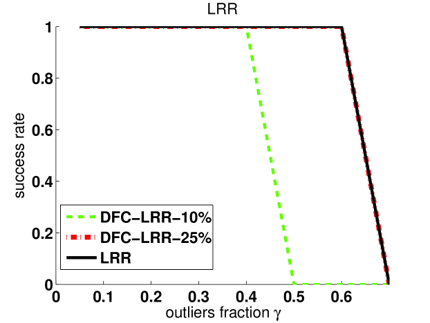
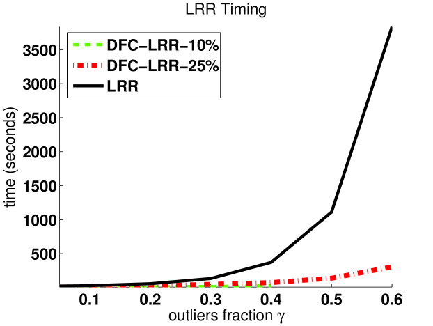
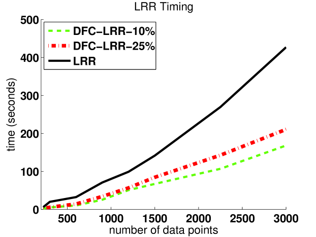
(a)	(b)	(c)

Figure 1: Results on synthetic data (reported results are averages over $10$ trials). (a) Phase transition of LRR and DFC-LRR. (b,c) Timing results of LRR and DFC-LRR as functions of $\gamma$ and $n$ respectively.

3.2 High Probability Subspace Segmentation

Our main theoretical result shows that, with high probability and under the same conditions that guarantee the accuracy of LRR, DFC-LRR also exactly recovers the row space of ${\mathbf{L}}_{0}$. Recall that in our independent subspace setting accurate row space recovery is tantamount to correct segmentation of the columns of ${\mathbf{L}}_{0}$. The proof of our result, which generalizes the LRR analysis of [18] to a broader class of optimization problems and adapts the DFC analysis of [21], can be found in the appendix.

Theorem 3.

Fix any failure probability $\delta>0$. Under the conditions of Thm, 2, let ${\hat{{\mathbf{Z}}}^{proj}}$ be a solution returned by DFC-LRR. Then there exists a constant $\gamma^{*}$ (depending on $\mu$ and $r$) for which the column space of ${\hat{{\mathbf{Z}}}^{proj}}$ exactly equals the row space of ${\mathbf{L}}_{0}$ whenever $\lambda=3/(7{\|{{\mathbf{M}}}\|}\sqrt{\gamma^{*}l})$ for each DFC-LRR subproblem, $\gamma\leq\gamma^{*}$, and $t=n/l$ for

$$l\geq cr\mu\log(4n/\delta)/(\gamma^{*}-\gamma)^{2}$$

and $c$ a fixed constant larger than 1.

Thm. 3 establishes that, like LRR, DFC-LRR can tolerate a constant fraction of its data points being corrupted and still recover the correct subspace segmentation of the clean data points with high probability. When the number of datapoints $n$ is large, solving LRR directly may be prohibitive, but DFC-LRR need only solve a collection of small, tractable subproblems. Indeed, Thm. 3 guarantees high probability recovery for DFC-LRR even when the subproblem size $l$ is logarithmic in $n$. The corresponding reduction in computational complexity allows DFC-LRR to scale to large problems with little sacrifice in accuracy.

Notably, this column sampling complexity is better than that established by [21] in the matrix factorization setting: we require O$(r\log n)$ columns sampled, while [21] requires in the worst case $\Omega(n)$ columns for matrix completion and $\Omega((r\log n)^{2})$ for robust matrix factorization.

4 Experiments

We now explore the empirical performance of DFC-LRR on a variety of simulated and real-world datasets, first for the traditional task of robust subspace segmentation and next for the more complex task of graph-based semi-supervised learning. Our experiments are designed to show the effectiveness of DFC-LRR both when the theory of Section 3 holds and when it is violated. Our synthetic datasets satisfy the theoretical assumptions of low rank, incoherence, and a small fraction of corrupted columns, while our real-world datasets violate these criteria.

For all of our experiments we use the inexact Augmented Lagrange Multiplier (ALM) algorithm of [17] as our base LRR algorithm. For the subspace segmentation experiments, we set the regularization parameter to the values suggested in previous works [18, 17], while in our semi-supervised learning experiments we set it to $1/\sqrt{\max{(m,n)}}$ as suggested in prior work. In all experiments we report parallel running times for DFC-LRR, i.e., the time of the longest running subproblem plus the time required to combine submatrix estimates via column projection. All experiments were implemented in Matlab. The simulation studies were run on an x$86$-$64$ architecture using a single $2.60$ Ghz core and $30$GB of main memory, while the real data experiments were performed on an x$86$-$64$ architecture equipped with a 2.67GHz 12-core CPU and 64GB of main memory.

4.1 Subspace Segmentation: LRR vs. DFC-LRR

We first aim to verify that DFC-LRR produces accuracy comparable to LRR in significantly less time, both in synthetic and real-world settings. We focus on the standard robust subspace segmentation task of identifying the subspace associated with each input datapoint.

4.1.1 Simulations

To construct our synthetic robust subspace segmentation datasets, we first generate $n_{s}$ datapoints from each of $k$ independent $r$-dimensional subspaces of $\mathbb{R}^{m}$, in a manner similar to [18]. For each subspace $i$, we independently select a basis ${\mathbf{U}}_{i}$ uniformly from all matrices in $\mathbb{R}^{m\times r}$ with orthonormal columns and a matrix ${\mathbf{T}}_{i}\in\mathbb{R}^{r\times n_{s}}$ of independent entries each distributed uniformly in $[0,1]$. We form the matrix ${\mathbf{X}}_{i}\in\mathbb{R}^{m\times n_{s}}$ of samples from subspace $i$ via ${\mathbf{X}}_{i}={\mathbf{U}}_{i}{\mathbf{T}}_{i}$ and let ${\mathbf{X}}_{0}\in\mathbb{R}^{m\times kn_{s}}=[{\mathbf{X}}_{1}\,\,\ldots\,\,{\mathbf{X}}_{k}]$. For a given outlier fraction $\gamma$ we next generate an additional $n_{o}=\frac{\gamma}{1-\gamma}kn_{s}$ independent outlier samples, denoted by ${\mathbf{S}}\in\mathbb{R}^{m\times n_{o}}$. Each outlier sample has independent $\mathcal{N}(0,\sigma^{2})$ entries, where $\sigma$ is the average absolute value of the entries of the $kn_{s}$ original samples. We create the input matrix ${\mathbf{M}}\in\mathbb{R}^{m\times n}$, where $n=kn_{s}+n_{o}$, as a random permutation of the columns of $[{\mathbf{X}}_{0}\quad{\mathbf{S}}]$.

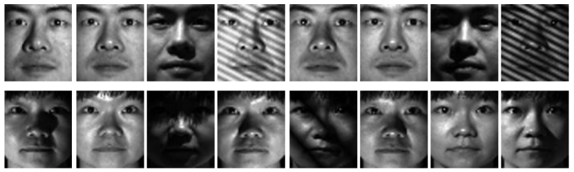
Figure 2: Exemplar face images from Extended Yale Database B. Each row shows randomly selected images for a human subject.

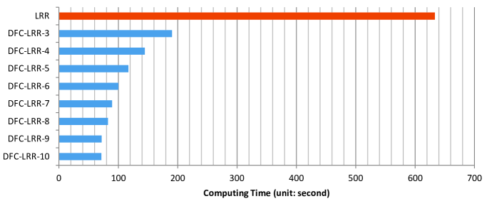
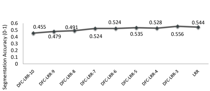
(a)	(b)

Figure 3: Trade-off between computation and segmentation accuracy on face recognition experiments. All results are obtained by averaging across 100 independent runs. (a) Run time of LRR and DFC-LRR with varying number of subproblems. (b) Segmentation accuracy for these same experiments.

In our first experiments we fix $k=3$, $m=1500$, $r=5$, and $n_{s}=200$, set the regularizer to $\lambda=0.2$, and vary the fraction of outliers. We measure with what frequency LRR and DFC-LRR are able to recover of the row space of ${\mathbf{X}}_{0}$ and identify the outlier columns in ${\mathbf{S}}$, using the same criterion as defined in [18]. Figure 1(a) shows average performance over $10$ trials. We see that DFC-LRR performs quite well, as the gaps in the phase transitions between LRR and DFC-LRR are small when sampling $10\%$ of the columns (i.e., $t=10$) and are virtually non-existent when sampling $25\%$ of the columns (i.e., $t=4$).

Figure 1(b) shows corresponding timing results for the accuracy results presented in Figure 1(a). These timing results show substantial speedups in DFC-LRR relative to LRR with a modest tradeoff in accuracy as denoted in Figure 1(a). Note that we only report timing results for values of $\gamma$ for which DFC-LRR was successful in all $10$ trials, i.e., for which the success rate equaled $1.0$ in Figure 1(a). Moreover, Figure 1(c) shows timing results using the same parameter values, except with a fixed fraction of outliers ($\gamma=0.1$) and a variable number of samples in each subspace, i.e., $n_{s}$ ranges from $75$ to $1000$. These timing results also show speedups with minimal loss of accuracy, as in all of these timing experiments, LRR and DFC-LRR were successful in all trials using the same criterion defined in [18] and used in our phase transition experiments of Figure 1(a).

4.1.2 Face Clustering

We next demonstrate the comparable quality and increased performance of DFC-LRR relative to LRR on real data, namely, a subset of Extended Yale Database B, a standard face benchmarking dataset. Following the experimental setup in [17], $640$ frontal face images of $10$ human subjects are chosen, each of which is resized to be $48\times 42$ pixels and forms a 2016-dimensional feature vector. As noted in previous work [3], a low-dimensional subspace can be effectively used to model face images from one person, and hence face clustering is a natural application of subspace segmentation. Moreover, as illustrated in Figure 2, a significant portion of the faces in this dataset are “corrupted” by shadows, and hence this collection of images is an ideal benchmark for robust subspace segmentation.

As in [17], we use the feature vector representation of these images to create a $2016\times 640$ dictionary matrix, ${\mathbf{M}}$, and run both LRR and DFC-LRR with the parameter $\lambda$ set to $0.15$. Next, we use the resulting low-rank coefficient matrix $\hat{{\mathbf{Z}}}$ to compute an affinity matrix ${\mathbf{U}}_{\hat{Z}}{\mathbf{U}}_{\hat{Z}}^{\top}$, where ${\mathbf{U}}_{\hat{Z}}$ contains the top left singular vectors of $\hat{{\mathbf{Z}}}$. The affinity matrix is used to cluster the data into $k=10$ clusters (corresponding to the $10$ human subjects) via spectral embedding (to obtain a $10$D feature representation) followed by $k$-means. Following [17], the comparison of different clustering methods relies on segmentation accuracy. Each of the $10$ clusters is assigned a label based on majority vote of the ground truth labels of the points assigned to the cluster. We evaluate clustering performance of both LRR and DFC-LRR by computing segmentation accuracy as in [17], i.e., each cluster is assigned a label based on majority vote of the ground truth labels of the points assigned to the cluster. The segmentation accuracy is then computed by averaging the percentage of correctly classified data over all classes.

Figures 3(a) and 3(b) show the computation time and the segmentation accuracy, respectively, for LRR and for DFC-LRR with varying numbers of subproblems (i.e., values of $t$). On this relatively-small data set ($n=640$ faces), LRR requires over $10$ minutes to converge. DFC-LRR demonstrates a roughly linear computational speedup as a function of $t$, comparable accuracies to LRR for smaller values of $t$ and a quite gradual decrease in accuracy for larger $t$.

4.2 Graph-based Semi-Supervised Learning

Graph representations, in which samples are vertices and weighted edges express affinity relationships between samples, are crucial in various computer vision tasks. Classical graph construction methods separately calculate the outgoing edges for each sample. This local strategy makes the graph vulnerable to contaminated data or outliers. Recent work in computer vision has illustrated the utility of global graph construction strategies using graph Laplacian [9] or matrix low-rank [32] based regularizers. L1 regularization has also been effectively used to encourage sparse graph construction [5, 13]. Building upon the success of global construction methods and noting the connection between subspace segmentation and graph construction as described in Section 2.1, we present a novel application of the low-rank representation methodology, relying on our DFC-LRR algorithm to scalably yield a sparse, low-rank graph (SLR-graph). We present a variety of results on large-scale semi-supervised learning visual classification tasks and provide a detailed comparison with leading baseline algorithms.

4.2.1 Benchmarking Data

We adopt the following three large-scale benchmarks:

Columbia Consumer Video (CCV) Content Detection: Compiled to stimulate research on recognizing highly-diverse visual content in unconstrained videos, this dataset consists of $9317$ YouTube videos over $20$ semantic categories (e.g., baseball, beach, music performance). Three popular audio/visual features (5000-D SIFT, 5000-D STIP, and 4000-D MFCC) are extracted.

MED12 Multimedia Event Detection: The MED12 video corpus consists of $\mathtt{\sim}150$K multimedia videos, with an average duration of $2$ minutes, and is used for detecting 20 specific semantic events. For each event, $130$ to $367$ videos are provided as positive examples, and the remainder of the videos are “null” videos that do not correspond to any event. In this work, we keep all positive examples and sample $10$K null videos, resulting in a dataset of $13,876$ videos. We extract six features from each video, first at sampled frames and then accumulated to obtain video-level representations. The features are either visual (1000-D sparse-SIFT, 1000-D dense-SIFT, 1500-D color-SIFT, 5000-D STIP), audio (2000-D MFCC), or semantic features (2659-D CLASSEME [25]).

NUS-WIDE-Lite Image Tagging: NUS-WIDE is among the largest available image tagging benchmarks, consisting of over $269$K crawled images from Flickr that are associated with over $5$K user-provided tags. Ground-truth images are manually provided for $81$ selected concept tags. We generate a lite version by sampling $20$K images. For each image, 128-D wavelet texture, 225-D block-wise LAB-based color moments and 500-D bag of visual words are extracted, normalized and finally concatenated to form a single feature representation for the image.

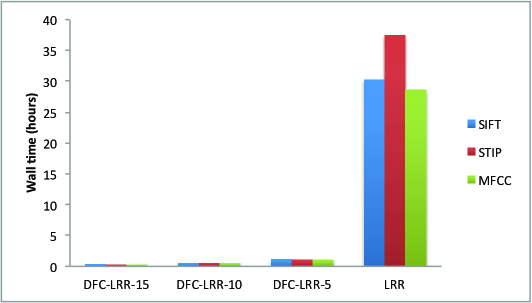
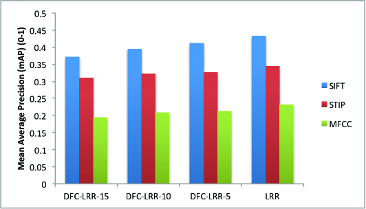
(a)	(b)

Figure 4: Trade-off between computation and accuracy for the SLR-graph on the CCV dataset. (a) Wall time of LRR and DFC-LRR with varying numbers of subproblems. (b) mAP scores for these same experiments.

4.2.2 Graph Construction Algorithms

The three graph construction schemes we evaluate are described below. Note that we exclude other baselines (e.g., NNLRS [32], LLE graph [28], L1-graph [5]) due to either scalability concerns or because prior work has already demonstrated inferior performance relative to the SPG algorithm defined below [32].

$k$NN-graph: We construct a nearest neighbor graph by connecting (via undirected edges) each vertex to its $k$ nearest neighbors in terms of $l_{2}$ distance in the specified feature space. Exponential weights are associated with edges, i.e., $w_{ij}=\operatorname{exp}\mathopen{}\mathclose{{}\left(-d_{ij}^{2}/\sigma^{2}}\right)$, where $d_{ij}$ is the distance between $x_{i}$ and $x_{j}$ and $\sigma$ is an empirically-tuned parameter [27].

SPG: Cheng et al. [5] proposed a noise-resistant L1-graph which encourages sparse vertex connectedness, motivated by the work of sparse representation [29]. Subsequent work, entitled sparse probability graph (SPG) [13] enforced positive graph weights. Following the approach of [32], we implemented a variant of SPG by solving the following optimization problem for each sample:

$$\min_{\mathbf{w}_{x}}\ \ \|\mathbf{x}-\mathbf{D}_{x}\mathbf{w}_{x}\|_{2}^{2}+\alpha\|\mathbf{w}_{x}\|_{1},\ \ s.t.\ \ \mathbf{w}_{x}\geq 0,$$ (3)

where $\mathbf{x}$ is a feature representation of a sample and $\mathbf{D}_{x}$ is the basis matrix for ${\mathbf{x}}$ constructed from its $n_{k}$ nearest neighbors. We use an open-source tool to solve this non-negative Lasso problem.

SLR-graph: Our novel graph construction method contains two-steps: first LRR or DFC-LRR is performed on the entire data set to recover the intrinsic low-rank clustering structure. We then treat the resulting low-rank coefficient matrix ${\mathbf{Z}}$ as an affinity matrix, and for sample $x_{i}$, the $n_{k}$ samples with largest affinities to $x_{i}$ are selected to form a basis matrix and used to solve the SPG optimization described by Problem (3). The resulting non-negative coefficients (typically sparse owing to the $\ell_{1}$ regularization term on $\mathbf{w}_{x}$ in  (3)) are used to define the graph.

Table 1: Mean average precision (mAP) (0-1) scores for various graph construction methods. DFC-LRR-10 is performed for SLR-Graph. The best mAP score for each feature is highlighted in bold.

(a) CCV

	$k$NN-Graph	SPG	SLR-Graph
SIFT	.2631	.3863	.3946
STIP	.2011	.3036	.3227
MFCC	.1420	.2129	.2085

(b) MED12

	$k$NN-Graph	SPG	SLR-Graph
Color-SIFT	.0742	.1202	.1432
Dense-SIFT	.0928	.1350	.1525
Sparse-SIFT	.0780	.1258	.1464
MFCC	.0962	.1371	.1371
CLASSEME	.1302	.1872	.2120
STIP	.0620	.0835	.0803

(c) NUS-WIDE-Lite

$k$NN-Graph	SPG	SLR-Graph
.1080	.1003	.1179

4.2.3 Experimental Design

For each benchmarking dataset, we first construct graphs by treating sample images/videos as vertices and using the three algorithms outlined in Section 4.2.2 to create (sparse) weighted edges between vertices. For fair comparison, we use the same parameter settings, namely $\alpha=0.05$ and $n_{k}=500$ for both SPG and SLR-graph. Moreover, we set $k=40$ for $k$NN-graph after tuning over the range $k=10$ through $k=60$.

We then use a given graph structure to perform semi-supervised label propagation using an efficient label propagation algorithm [27] that enjoys a closed-form solution and often achieves the state-of-the-art performance. We perform a separate label propagation for each category in our benchmark, i.e., we run a series of $20$ binary classification label propagation experiments for CCV/MED12 and $81$ experiments for NUS-WIDE-Lite. For each category, we randomly select half of the samples as training points (and use their ground truth labels for label propagation) and use the remaining half as a test set. We repeat this process $20$ times for each category with different random splits. Finally, we compute Mean Average Precision (mAP) based on the results on the test sets across all runs of label propagation.

4.2.4 Experimental Results

We first performed experiments using the CCV benchmark, the smallest of our datasets, to explore the tradeoff between computation and accuracy when using DFC-LRR as part of our proposed SLR-graph. Figure 4(a) presents the time required to run SLR-graph with LRR versus DFC-LRR with three different numbers of subproblems ($t=5,10,15$), while Figure 4(b) presents the corresponding accuracy results. The figures show that DFC-LRR performs comparably to LRR for smaller values of $t$, and performance gradually degrades for larger $t$. Moreover, DFC-LRR is up to two orders of magnitude faster and achieves superlinear speedups relative to LRR. Given the scalability issues of LRR on this modest-sized dataset, along with the comparable accuracy of DFC-LRR, we ran SLR-graph exclusively with DFC-LRR ($t=10$) for our two larger datasets.

Table 1 summarizes the results of our semi-supervised learning experiments using the three graph construction techniques defined in Section 4.2.2. The results show that our proposed SLR-graph approach leads to significant performance gains in terms of mAP across all benchmarking datasets for the vast majority of features. These results demonstrate the benefit of enforcing both low-rankedness and sparsity during graph construction. Moreover, conventional low-rank oriented algorithms, e.g., [32, 16] would be computationally infeasible on our benchmarking datasets, thus highlighting the utility of employing DFC’s divide-and-conquer approach to generate a scalable algorithm.

5 Conclusion

Our primary goal in this work was to introduce a provably accurate algorithm suitable for large-scale low-rank subspace segmentation. While some contemporaneous work [1] also aims at scalable subspace segmentation, this method offers no guarantee of correctness. In contrast, DFC-LRR provably preserves the theoretical recovery guarantees of the LRR program. Moreover, our divide-and-conquer approach achieves empirical accuracy comparable to state-of-the-art methods while obtaining linear to superlinear computational gains, both on standard subspace segmentation tasks and on novel applications to semi-supervised learning. DFC-LRR also lays the groundwork for scaling up LRR derivatives known to offer improved performance, e.g., LatLRR in the setting of standard subspace segmentation and NNLRS in the graph-based semi-supervised learning setting. The same techniques may prove useful in developing scalable approximations to other convex formulations for subspace segmentation, e.g., [20].

Appendix A Proof of Theorem 3

Our proof of Thm. 3 rests upon three key results: a new deterministic recovery guarantee for LRR-type problems that generalizes the guarantee of [18], a probabilistic estimation guarantee for column projection established in [21], and a probabilistic guarantee of [21] showing that a uniformly chosen submatrix of a $(\mu,r)$-coherent matrix is nearly $(\mu,r)$-coherent. These results are presented in Secs. A.1, A.2, and A.3 respectively. The proof of Thm. 3 follows in Sec. A.4.

In what follows, the unadorned norm ${\|{\cdot}\|}$ represents the spectral norm of a matrix. We will also make use of a technical condition, introduced by Liu et al. [18] to ensure that a corrupted data matrix is well-behaved when used as a dictionary:

Definition 4 (Relatively Well-Definedness).

A matrix ${\mathbf{M}}={\mathbf{L}}_{0}+{\mathbf{S}}_{0}$ is $\beta$-RWD if

$${\|{{\mathbf{\Sigma}}_{M}^{-1}{\mathbf{V}}_{M}^{T}{\mathbf{V}}_{L_{0}}}\|}\leq\frac{1}{\beta{\|{{\mathbf{M}}}\|}}.$$

A larger value of $\beta$ corresponds to improved recovery properties.

A.1 Analysis of Low-Rank Representation

Thm. 1 of [18] analyzes LRR recovery under the constraint $\mathbf{O}={\mathbf{D}}{\mathbf{Z}}+{\mathbf{S}}$ when the observation matrix $\mathbf{O}$ and the dictionary ${\mathbf{D}}$ are both equal to the input matrix ${\mathbf{M}}$. Our next theorem provides a comparable analysis when the observation matrix is a column submatrix of the dictionary.

Theorem 5.

Suppose that ${\mathbf{M}}={\mathbf{L}}_{0}+{\mathbf{S}}_{0}\in\mathbb{R}^{m\times n}$ is $\beta$-RWD with rank $r$ and that ${\mathbf{L}}_{0}$ and ${\mathbf{S}}_{0}$ have independent column support with ${\rm range}({{\mathbf{L}}_{0}})\cap{\rm range}({{\mathbf{S}}_{0}})=\{\mathbf{0}\}$. Let ${\mathbf{S}}_{0,C}\in\mathbb{R}^{m\times l}$ be a column submatrix of ${\mathbf{S}}_{0}$ supported on $\gamma l$ columns, and suppose that ${\mathbf{C}}$, the corresponding column submatrix of ${\mathbf{M}}$, is $(\frac{\mu}{1-\gamma},r)$-coherent. Define

$$\gamma^{*}\triangleq\frac{324\beta^{2}}{324\beta^{2}+49(11+4\beta)^{2}\mu r},$$

and let $(\hat{\mathbf{Z}},\hat{\mathbf{S}})$ be a solution to the problem

$$\min_{{\mathbf{Z}},{\mathbf{S}}}\quad{\|{{\mathbf{Z}}}\|}_{*}+\lambda{\|{{\mathbf{S}}}\|}_{2,1}\quad\text{subject\, to}\quad{\mathbf{C}}={\mathbf{M}}{\mathbf{Z}}+{\mathbf{S}}$$ (4)

with $\lambda=3/(7{\|{{\mathbf{M}}}\|}\sqrt{\gamma^{*}l})$. If $\gamma\leq\gamma^{*}$, then the column space of $\hat{\mathbf{Z}}$ equals the row space of ${\mathbf{L}}_{0}$.

The proof of Thm. 5 can be found in Sec. B.

A.2 Analysis of Column Projection

The following lemma, due to [21], shows that, with high probability, column projection exactly recovers a $(\mu,r)$-coherent matrix by sampling a number of columns proportional to $\mu r\log n$.

Corollary 6 (Column Projection under Incoherence [21, Cor. 6]).

Let ${\mathbf{L}}\in\mathbb{R}^{m\times n}$ be $(\mu,r)$-coherent, and let ${\mathbf{L}}_{C}\in\mathbb{R}^{m\times l}$ be a matrix of $l$ columns of ${\mathbf{L}}$ sampled uniformly without replacement. If $l\geq cr\mu\log(n)\log(1/\delta),$ where $c$ is a fixed positive constant, then,

$${\mathbf{L}}={\mathbf{L}}^{proj}\triangleq{\mathbf{U}}_{L_{C}}{\mathbf{U}}_{L_{C}}^{\top}{\mathbf{L}}$$

exactly with probability at least $1-\delta$.

A.3 Conservation of Incoherence

The following lemma of [21] shows that, with high probability, ${\mathbf{L}}_{0,i}$ captures the full rank of ${\mathbf{L}}_{0}$ and has coherence not much larger than $\mu$.

Lemma 7 (Conservation of Incoherence [21, Lem. 7]).

Let ${\mathbf{L}}\in\mathbb{R}^{m\times n}$ be $(\mu,r)$-coherent, and let ${\mathbf{L}}_{C}\in\mathbb{R}^{m\times l}$ be a matrix of $l$ columns of ${\mathbf{L}}$ sampled uniformly without replacement. If $l\geq cr\mu\log(n)\log(1/\delta)/\epsilon^{2},$ where $c$ is a fixed constant larger than 1, then ${\mathbf{L}}_{C}$ is $(\frac{\mu}{1-\epsilon/2},r)$-coherent with probability at least $1-\delta/n$.

A.4 Proof of DFC-LRR Guarantee

Recall that, under Alg. 1, the input matrix ${\mathbf{M}}$ has been partitioned into column submatrices $\{{\mathbf{C}}_{1},\dots,{\mathbf{C}}_{t}\}$. Let $\{{\mathbf{C}}_{0,1},\dots,{\mathbf{C}}_{0,t}\}$ and $\{{\mathbf{S}}_{0,1},\dots,{\mathbf{S}}_{0,t}\}$ be the corresponding partitions of ${\mathbf{L}}_{0}$ and ${\mathbf{S}}_{0}$, let $s_{i}\triangleq\gamma_{i}l$ be the size of the column support of ${\mathbf{S}}_{0,i}$ for each index $i$, and let $(\hat{\mathbf{Z}}_{i},\hat{\mathbf{S}}_{i})$ be a solution to the $i$th DFC-LRR subproblem.

For each index $i$, we further define $A_{i}$ as the event that ${\mathbf{C}}_{0,i}$ is $(4\mu/(1-\gamma_{i}),r)$-coherent, $B_{i}$ as the event that $s_{i}\leq\gamma^{*}l$, and $G({\mathbf{Z}})$ as the event that the column space of the matrix ${\mathbf{Z}}$ is equal to the row space of ${\mathbf{L}}_{0}$. Under our choice of $\gamma^{*}$, Thm. 5 implies that $G(\hat{\mathbf{Z}}_{i})$ holds when $A_{i}$ and $B_{i}$ are both realized. Hence, when $A_{i}$ and $B_{i}$ hold for all indices $i$, the column space of $\hat{\mathbf{Z}}=[\hat{\mathbf{Z}}_{1},\dots,\hat{\mathbf{Z}}_{t}]$ precisely equals the row space of ${\mathbf{L}}_{0}$, and the median rank of $\{\hat{\mathbf{Z}}_{1},\dots,\hat{\mathbf{Z}}_{t}\}$ equals $r$.

Applying Cor. 6 with

$$l\geq cr\mu\log^{2}(4n/\delta)/(\gamma^{*}-\gamma)^{2}\geq cr\mu\log(n)\log(4/\delta),$$

shows that, given $A_{i}$ and $B_{i}$ for all indices $i$, ${\hat{{\mathbf{Z}}}^{proj}}$ equals $\hat{\mathbf{Z}}$ with probability at least $1-\delta/4$. To establish $G({\hat{{\mathbf{Z}}}^{rp}})$ with probability at least $1-\delta$, it therefore remains to show that

$${\mathbf{P}}\mathopen{}\mathclose{{}\left({\cap_{i=1}^{t}(A_{i}\cap B_{i})}}\right) =1-{\mathbf{P}}\mathopen{}\mathclose{{}\left({\cup_{i=1}^{t}(A_{i}^{c}\cup B_{i}^{c})}}\right)$$ (5)

$$\geq 1-\sum_{i=1}^{t}({\mathbf{P}}\mathopen{}\mathclose{{}\left({A_{i}^{c}}}\right)+{\mathbf{P}}\mathopen{}\mathclose{{}\left({B_{i}^{c}}}\right))$$ (6)

$$\geq 1-3\delta/4.$$ (7)

Because DFC-LRR partitions columns uniformly at random, the variable $s_{i}$ has a hypergeometric distribution with $\mathrm{E}{s_{i}}=\gamma l$ and therefore satisfies Hoeffding’s inequality for the hypergeometric distribution [14, Sec. 6]:

$${\mathbf{P}}\mathopen{}\mathclose{{}\left({s_{i}\geq\mathrm{E}{s_{i}}+l\tau}}\right)\leq\operatorname{exp}\mathopen{}\mathclose{{}\left(-2lt^{2}}\right).$$

It follows that

$${\mathbf{P}}\mathopen{}\mathclose{{}\left({B_{i}^{c}}}\right)={\mathbf{P}}\mathopen{}\mathclose{{}\left({s_{i}>\gamma^{*}l}}\right) ={\mathbf{P}}\mathopen{}\mathclose{{}\left({s_{i}>\mathrm{E}s_{i}+l(\gamma^{*}-\gamma)}}\right)$$

$$\leq\operatorname{exp}\mathopen{}\mathclose{{}\left(-2l(\gamma^{*}-\gamma)^{2}}\right)\leq\delta/(4t)$$

by our assumption that $l\geq cr\mu\log^{2}(4n/\delta)/(\gamma^{*}-\gamma)^{2}\geq\log(4t/\delta)/[2(\gamma^{*}-\gamma)^{2}]$.

By Lem. 7 and our choice of

$$l \geq cr\mu\log^{2}(4n/\delta)/(\gamma^{*}-\gamma)^{2}$$

$$\geq cr\mu\log(n)\log(4/\delta)/(1-\gamma),$$

each submatrix ${\mathbf{C}}_{0,i}$ is $(2\mu/(1-\gamma),r)$-coherent with probability at least $1-\delta/(4n)\geq 1-\delta/(4t)$. A second application of Hoeffding’s inequality for the hypergeometric further implies that

$${\mathbf{P}}\mathopen{}\mathclose{{}\left({\frac{2\mu}{1-\gamma}>\frac{4\mu}{1-\gamma_{i}}}}\right) ={\mathbf{P}}\mathopen{}\mathclose{{}\left({s_{i}<\mathrm{E}s_{i}-l(1-\gamma)}}\right)$$

$$\leq\operatorname{exp}\mathopen{}\mathclose{{}\left(-2l(1-\gamma)^{2}}\right)$$

$$\leq\delta/(4t),$$

since $l\geq cr\mu\log(4n/\delta)/(\gamma^{*}-\gamma)^{2}\geq\log(4t/\delta)/[2(1-\gamma)^{2}]$. Hence, ${\mathbf{P}}\mathopen{}\mathclose{{}\left({A_{i}^{c}}}\right)\leq\delta/(2t)$.

Combining our results, we find

$$\sum_{i=1}^{t}({\mathbf{P}}\mathopen{}\mathclose{{}\left({A_{i}^{c}}}\right)+{\mathbf{P}}\mathopen{}\mathclose{{}\left({B_{i}^{c}}}\right))\leq 3\delta/4$$

as desired.

Appendix B Proof of Theorem 5

Let $\mathcal{I}_{0}$ be the column support of ${\mathbf{S}}_{0,C}$, and let $\mathcal{I}_{0}^{c}$ be its set complement in $\{1,\dots,l\}$. For any matrix ${\mathbf{S}}\in\mathbb{R}^{a\times b}$ and index set $\mathcal{I}\subseteq\{1,\dots,b\}$, we let ${\mathcal{P}}_{\mathcal{I}}({\mathbf{S}})$ be the orthogonal projection of ${\mathbf{S}}$ onto the space of $a\times b$ matrices with column support $\mathcal{I}$, so that $({\mathcal{P}}_{\mathcal{I}}({\mathbf{S}}))^{(j)}={\mathbf{S}}^{(j)},\ \text{if}\ j\in\mathcal{I}\quad\text{and}\quad({\mathcal{P}}_{\mathcal{I}}({\mathbf{S}}))^{(j)}=\mathbf{0}\ \text{otherwise}.$

B.1 Oracle Constraints

Our proof of Thm. 5 will parallel Thm. 1 of [18]. We begin by introducing two oracle constraints that would guarantee the desired outcome if satisfied.

Lemma 8.

Under the assumptions of Thm. 5, suppose that ${\mathbf{C}}={\mathbf{M}}{\mathbf{Z}}+{\mathbf{S}}$ for some matrices $({\mathbf{Z}},{\mathbf{S}})$. If $({\mathbf{Z}},{\mathbf{S}})$ additionally satisfy the oracle constraints

$${\mathbf{P}}_{L_{0}^{\top}}{\mathbf{Z}}={\mathbf{Z}}\quad\text{and}\quad{\mathcal{P}}_{\mathcal{I}_{0}}({\mathbf{S}})={\mathbf{S}}$$ (8)

then the column space of ${\mathbf{Z}}$ equals the row space of ${\mathbf{L}}_{0}$.

Proof    By Eq. 8, the row space of ${\mathbf{L}}_{0}$ contains the column space of ${\mathbf{Z}}$, so the two will be equal if $\mathrm{rank}({{\mathbf{L}}_{0}})=\mathrm{rank}({{\mathbf{Z}}})$. This equality indeed holds, since

$${\mathbf{C}}_{0}={\mathcal{P}}_{\mathcal{I}_{0}^{c}}({\mathbf{C}})={\mathcal{P}}_{\mathcal{I}_{0}^{c}}({\mathbf{M}}{\mathbf{Z}}+{\mathbf{S}})={\mathbf{M}}{\mathcal{P}}_{\mathcal{I}_{0}^{c}}({\mathbf{Z}}),$$

and therefore $\mathrm{rank}({{\mathbf{L}}_{0}})=\mathrm{rank}({{\mathbf{C}}_{0}})\leq\mathrm{rank}({{\mathbf{M}}{\mathcal{P}}_{\mathcal{I}_{0}^{c}}({\mathbf{Z}})})\leq\mathrm{rank}({{\mathcal{P}}_{\mathcal{I}_{0}^{c}}({\mathbf{Z}})})\leq\mathrm{rank}({{\mathbf{Z}}})\leq\mathrm{rank}({{\mathbf{L}}_{0}}).$ ∎
Thus, to prove Thm. 5, it suffices to show that any solution to Eq. 4 also satisfies the oracle constraints of Eq. 8.

B.2 Conditions for Optimality

To this end, we derive sufficient conditions for solving Eq. 4 and moreover show that if any solution to Eq. 4 satisfies the oracle constraints of Eq. 8, then all solutions do.

We will require some additional notation. For a matrix ${\mathbf{Z}}\in\mathbb{R}^{n\times l}$ we define $T({\mathbf{Z}})\triangleq\{{\mathbf{U}}_{Z}{\mathbf{X}}+{\mathbf{Y}}{\mathbf{V}}_{Z}^{\top}:{\mathbf{X}}\in\mathbb{R}^{r\times l},{\mathbf{Y}}\in\mathbb{R}^{n\times r}\}$, ${\mathcal{P}}_{T({\mathbf{Z}})}$ as the orthogonal projection onto the set $T({\mathbf{Z}})$, and ${\mathcal{P}}_{T({\mathbf{Z}})^{\bot}}$ as the orthogonal projection onto the orthogonal complement of $T({\mathbf{Z}})$. For a matrix ${\mathbf{S}}$ with column support $\mathcal{I}$, we define the column normalized version, $\mathcal{B}({\mathbf{S}})$, which satisfies

$${\mathcal{P}}_{\mathcal{I}^{c}}(\mathcal{B}({\mathbf{S}}))=\mathbf{0}\quad\text{and}\quad\mathcal{B}({\mathbf{S}})^{(j)}\triangleq{\mathbf{S}}^{(j)}/{\|{{\mathbf{S}}^{(j)}}\|}\quad\forall j\in\mathcal{I}.$$

Theorem 9.

Under the assumptions of Thm. 5, suppose that ${\mathbf{C}}={\mathbf{M}}{\mathbf{Z}}+{\mathbf{S}}$ for some matrices $({\mathbf{Z}},{\mathbf{S}})$. If there exists a matrix ${\mathbf{Q}}$ satisfying

1. ${\mathcal{P}}_{T({\mathbf{Z}})}({\mathbf{M}}^{\top}{\mathbf{Q}})={\mathbf{U}}_{Z}{\mathbf{V}}_{Z}^{\top}$

2. ${\|{{\mathcal{P}}_{T({\mathbf{Z}})^{\bot}}({\mathbf{M}}^{\top}{\mathbf{Q}})}\|}<1$

3. ${\mathcal{P}}_{\mathcal{I}_{0}}({\mathbf{Q}})=\lambda\mathcal{B}({\mathbf{S}})$

4. ${\|{{\mathcal{P}}_{\mathcal{I}_{0}^{c}}({\mathbf{Q}})}\|}_{2,\infty}<\lambda.$

then $({\mathbf{Z}},{\mathbf{S}})$ is a solution to Eq. 4. If, in addition, ${\mathcal{P}}_{\mathcal{I}_{0}}({\mathbf{Z}}^{+}{\mathbf{Z}})=\mathbf{0}$, and $({\mathbf{Z}},{\mathbf{S}})$ satisfy the oracle constraints of Eq. 8, then all solutions to Eq. 4 satisfy the oracle constraints of Eq. 8.

Proof    The proof of this theorem is identical to that of [18, Thm. 3] which establishes the same result when the observation ${\mathbf{C}}$ is replaced by ${\mathbf{M}}$. ∎
It remains to construct a feasible pair $({\mathbf{Z}},{\mathbf{S}})$ satisfying the oracle constraints and ${\mathcal{P}}_{\mathcal{I}_{0}}({\mathbf{Z}}^{+}{\mathbf{Z}})=\mathbf{0}$ and a dual certificate ${\mathbf{Q}}$ satisfying the conditions of Thm. 9.

B.3 Constructing a Dual Certificate

To this end, we consider the oracle problem:

$$\min_{{\mathbf{Z}},{\mathbf{S}}}\quad{\|{{\mathbf{Z}}}\|}_{*}+\lambda{\|{{\mathbf{S}}}\|}_{2,1}\quad$$ (9)

subject  to

$${\mathbf{C}}={\mathbf{M}}{\mathbf{Z}}+{\mathbf{S}},\quad{\mathbf{P}}_{L_{0}^{\top}}{\mathbf{Z}}={\mathbf{Z}},\quad\text{and}\quad{\mathcal{P}}_{\mathcal{I}_{0}}({\mathbf{S}})={\mathbf{S}}.$$

Let ${\mathbf{Y}}$ be the binary matrix that selects the columns of ${\mathbf{C}}$ from ${\mathbf{M}}$. Then $({\mathbf{P}}_{L_{0}^{\top}}{\mathbf{Y}},{\mathbf{S}}_{0,i})$ is feasible for this problem, and hence an optimal solution $({\mathbf{Z}}^{*},{\mathbf{S}}^{*})$ must exist. By explicitly constructing a dual certificate ${\mathbf{Q}}$, we will show that $({\mathbf{Z}}^{*},{\mathbf{S}}^{*})$ also solves the LRR subproblem of Eq. 4.

We will need a variety of lemmas paralleling those developed in [18]. Let

$$\bar{\mathbf{V}}\triangleq{\mathbf{V}}_{Z^{*}}{\mathbf{U}}_{Z^{*}}^{\top}{\mathbf{V}}_{L_{0}}.$$

The following lemma was established in [18].

Lemma 10 (Lem. 8 of [18]).

$\bar{\mathbf{V}}\bar{\mathbf{V}}^{\top}={\mathbf{V}}_{Z^{*}}{\mathbf{V}}_{Z^{*}}^{\top}$. Moreover, for any ${\mathbf{A}}\in\mathbb{R}^{m\times l}$,

$${\mathcal{P}}_{T({\mathbf{Z}}^{*})}({\mathbf{A}})={\mathbf{P}}_{L_{0}^{\top}}{\mathbf{A}}+{\mathbf{A}}{\mathbf{P}}_{\bar{\mathbf{V}}}-{\mathbf{P}}_{L_{0}^{\top}}{\mathbf{A}}{\mathbf{P}}_{\bar{\mathbf{V}}}.$$

The next lemma parallels Lem. 9 of [18].

Lemma 11.

Let $\hat{\mathbf{H}}=\mathcal{B}({\mathbf{S}}^{*})$. Then

$${\mathbf{V}}_{L_{0}}{\mathcal{P}}_{\mathcal{I}_{0}}(\bar{\mathbf{V}}^{\top})=\lambda{\mathbf{P}}_{L_{0}^{\top}}{\mathbf{M}}^{\top}\hat{\mathbf{H}}.$$

Proof    The proof is identical to that of Lem. 9 of [18]. ∎

Define

$${\mathbf{G}}\triangleq{\mathcal{P}}_{\mathcal{I}_{0}}(\bar{\mathbf{V}}^{\top})({\mathcal{P}}_{\mathcal{I}_{0}}(\bar{\mathbf{V}}^{\top}))^{\top}\quad\text{and}\quad\psi\triangleq{\|{{\mathbf{G}}}\|}.$$

The next lemma parallels Lem. 10 of [18].

Lemma 12.

$\psi\leq\lambda^{2}{\|{{\mathbf{M}}}\|}^{2}\gamma l$.

Proof    The proof is identical to that of Lem. 10 of [18], save for the size of $\mathcal{I}_{0}$, which is now bounded by $\gamma l$. ∎
Note that under the assumption $\lambda\leq 3/(7{\|{{\mathbf{M}}}\|}\sqrt{\gamma l})$, we have $\psi\leq 1/4$.

The next lemma was established in [18].

Lemma 13 (Lem. 11 of [18]).

If $\psi<1$, then ${\mathcal{P}}_{\mathcal{I}_{0}}(({\mathbf{Z}}^{*})^{+}{\mathbf{Z}}^{*})={\mathcal{P}}_{\mathcal{I}_{0}}({\mathbf{P}}_{\bar{V}})=\mathbf{0}$.

Lem. 12 of [18] is unchanged in our setting. The next lemma parallels Lem. 13 of [18].

Lemma 14.

${\|{{\mathcal{P}}_{\mathcal{I}_{0}^{c}}(\bar{\mathbf{V}}^{\top})}\|}_{2,\infty}\leq\sqrt{\frac{\mu r}{(1-\gamma)l}}$

Proof    By assumption, ${\mathbf{C}}={\mathbf{M}}{\mathbf{Z}}^{*}+{\mathbf{S}}^{*}$, $\mathrm{rank}({{\mathbf{C}}_{0}})=r$, and ${\mathcal{P}}_{\mathcal{I}_{0}^{c}}({\mathbf{C}})={\mathbf{C}}_{0}={\mathcal{P}}_{\mathcal{I}_{0}^{c}}({\mathbf{C}}_{0})$. Hence, ${\mathbf{C}}_{0}={\mathcal{P}}_{\mathcal{I}_{0}^{c}}({\mathbf{C}}_{0})={\mathbf{M}}{\mathcal{P}}_{\mathcal{I}_{0}^{c}}({\mathbf{Z}}^{*})$, and thus

$${\mathbf{V}}_{C_{0}}^{\top}={\mathcal{P}}_{\mathcal{I}_{0}^{c}}({\mathbf{V}}_{C_{0}}^{\top})={\mathbf{\Sigma}}_{C_{0}}^{-1}{\mathbf{U}}_{C_{0}}^{\top}{\mathbf{M}}{\mathbf{U}}_{Z^{*}}{\mathbf{\Sigma}}_{Z^{*}}{\mathcal{P}}_{\mathcal{I}_{0}^{c}}({\mathbf{V}}_{Z^{*}}^{\top}).$$

This relationship implies that

$$r=\mathrm{rank}({{\mathbf{V}}_{C_{0}}^{\top}})\leq\mathrm{rank}({{\mathcal{P}}_{\mathcal{I}_{0}^{c}}({\mathbf{V}}_{Z^{*}}^{\top})})\leq\mathrm{rank}({{\mathbf{V}}_{Z^{*}}^{\top}})=r$$

and therefore that ${\mathcal{P}}_{\mathcal{I}_{0}^{c}}({\mathbf{V}}_{Z^{*}}^{\top})$ is of full row rank. The remainder of the proof is identical to that of Lem. 13 of [18], save for the coherence factor of $(1-\gamma)l$ in place of $(1-\gamma)n$. ∎

With these lemmas in hand, we define

$${\mathbf{Q}}_{1} \triangleq\lambda{\mathbf{P}}_{L_{0}^{\top}}{\mathbf{M}}^{\top}\hat{\mathbf{H}}={\mathbf{V}}_{L_{0}}{\mathcal{P}}_{\mathcal{I}_{0}}(\bar{\mathbf{V}}^{\top})$$

$${\mathbf{Q}}_{2} \triangleq\lambda{\mathbf{P}}_{(L_{0}^{\top})^{\bot}}{\mathcal{P}}_{\mathcal{I}_{0}^{c}}(({\mathbf{I}}+\sum_{i=1}^{\infty}({\mathbf{P}}_{\bar{V}}{\mathcal{P}}_{\mathcal{I}_{0}}{\mathbf{P}}_{\bar{V}})^{i}){\mathbf{P}}_{\bar{V}}){\mathbf{M}}\hat{\mathbf{H}}{\mathbf{P}}_{\bar{V}}$$

$$=\lambda{\mathcal{P}}_{\mathcal{I}_{0}^{c}}(({\mathbf{I}}+\sum_{i=1}^{\infty}({\mathbf{P}}_{\bar{V}}{\mathcal{P}}_{\mathcal{I}_{0}}{\mathbf{P}}_{\bar{V}})^{i}){\mathbf{P}}_{\bar{V}}){\mathbf{P}}_{(L_{0}^{\top})^{\bot}}{\mathbf{M}}\hat{\mathbf{H}}{\mathbf{P}}_{\bar{V}},$$

where the first relation follows from Lem. 11. Our final theorem parallels Thm. 4 of [18].

Theorem 15.

Assume $\psi<1$, and let

$${\mathbf{Q}}\triangleq({\mathbf{M}}^{+})^{\top}({\mathbf{V}}_{L_{0}}\bar{\mathbf{V}}^{\top}+\lambda{\mathbf{M}}^{\top}\hat{\mathbf{H}}-{\mathbf{Q}}_{1}-{\mathbf{Q}}_{2}).$$

If

$$\frac{\gamma}{1-\gamma}<\frac{\beta^{2}(1-\psi)^{2}}{(3-\psi+\beta)^{2}\mu r}\,,$$

$$\frac{(1-\psi)\sqrt{\frac{\mu r}{1-\gamma}}}{{\|{{\mathbf{M}}}\|}\sqrt{l}(\beta(1-\psi)-(1+\beta)\sqrt{\frac{\gamma}{1-\gamma}\mu r})}<\lambda\,,$$

and

$$\lambda<\frac{1-\psi}{{\|{{\mathbf{M}}}\|}\sqrt{\gamma l}(2-\psi)},$$

then ${\mathbf{Q}}$ satisfies the conditions in Thm. 9.

Proof    The proof of property $\mathbf{S3}$ requires a small modification. Thm. 4 of [18] establishes that ${\mathcal{P}}_{\mathcal{I}_{0}}({\mathbf{Q}})=\lambda{\mathbf{P}}_{M}\hat{\mathbf{H}}$. To conclude that ${\mathcal{P}}_{\mathcal{I}_{0}}({\mathbf{Q}})=\lambda\hat{\mathbf{H}}$, we note that ${\mathbf{S}}_{i}^{*}={\mathbf{C}}-{\mathbf{M}}{\mathbf{Z}}^{*}$ and that the column space of ${\mathbf{C}}$ contains the column space of ${\mathbf{M}}$ by assumption. Hence, ${\mathbf{P}}_{M}{\mathbf{S}}_{i}^{*}={\mathbf{S}}_{i}^{*}$ and therefore ${\mathcal{P}}_{\mathcal{I}_{0}}({\mathbf{Q}})=\lambda{\mathbf{P}}_{M}\hat{\mathbf{H}}=\lambda\hat{\mathbf{H}}$.

The proofs of properties $\mathbf{S4}$ and $\mathbf{S5}$ are unchanged except for the dimensionality factor which changes from $n$ to $l$. ∎

Finally, Lem. 14 of [18] guarantees that the preconditions of Thm. 15 are met under our assumptions on $\lambda,\gamma^{*},$ and $\gamma$.

References

- [1] A. Adler, M. Elad, and Y. Hel-Or. Probabilistic subspace clustering via sparse representations. IEEE Signal Process. Lett., 20(1):63–66, 2013.
- [2] R. Basri and D. Jacobs. Robust face recognition via sparse representation. IEEE Trans. Pattern Anal. Mach. Intell., 25(3):218–233, 2003.
- [3] E. J. Candès, X. Li, Y. Ma, and J. Wright. Robust principal component analysis? Journal of the ACM, 58(3):1–37, 2011.
- [4] B. Cheng, G. Liu, J. Wang, Z. Huang, and S. Yan. Multi-task low-rank affinity pursuit for image segmentation. In ICCV, 2011.
- [5] B. Cheng, J. Yang, S. Yan, Y. Fu, and T. S. Huang. Learning with l1-graph for image analysis. IEEE Transactions on Image Processing, 19(4):858–866, 2010.
- [6] J. Costeira and T. Kanade. A multibody factorization method for independently moving objects. International Journal of Computer Vision, 29(3), 1998.
- [7] E. Elhamifar and R. Vidal. Sparse subspace clustering. In CVPR, 2009.
- [8] B. R. Feng Niu, C. Ré, and S. J. Wright. Hogwild!: A lock-free approach to parallelizing stochastic gradient descent. In NIPS, 2011.
- [9] S. Gao, I. W. H. Tsang, L. T. Chia, and P. Zhao. Local features are not lonely - laplacian sparse coding for image classification. In CVPR, 2010.
- [10] C. W. Gear. Multibody grouping from motion images. Int. J. Comput. Vision, 29:133–150, August 1998.
- [11] R. Gemulla, E. Nijkamp, P. J. Haas, and Y. Sismanis. Large-scale matrix factorization with distributed stochastic gradient descent. In KDD, 2011.
- [12] T. Hastie and P. Simard. Metrics and models for handwritten character recognition. Statistical Science, 13(1):54–65, 1998.
- [13] R. He, W.-S. Zheng, B.-G. Hu, and X.-W. Kong. Nonnegative sparse coding for discriminative semi-supervised learning. In CVPR, 2011.
- [14] W. Hoeffding. Probability inequalities for sums of bounded random variables. Journal of the American Statistical Association, 58(301):13–30, 1963.
- [15] S. Kumar, M. Mohri, and A. Talwalkar. On sampling-based approximate spectral decomposition. In ICML, 2009.
- [16] Z. Lin, A. Ganesh, J. Wright, L. Wu, M. Chen, and Y. Ma. Fast convex optimization algorithms for exact recovery of a corrupted low-rank matrix. UIUC Technical Report UILU-ENG-09-2214, 2009.
- [17] G. Liu, Z. Lin, and Y. Yu. Robust subspace segmentation by low-rank representation. In ICML, 2010.
- [18] G. Liu, H. Xu, and S. Yan. Exact subspace segmentation and outlier detection by low-rank representation. arXiv:1109.1646v2[cs.IT], 2011.
- [19] G. Liu and S. Yan. Latent low-rank representation for subspace segmentation and feature extraction. In ICCV, 2011.
- [20] G. Liu and S. Yan. Active subspace: Toward scalable low-rank learning. Neural Computation, 24:3371–3394, 2012.
- [21] L. Mackey, A. Talwalkar, and M. I. Jordan. Divide-and-conquer matrix factorization. In NIPS, 2011.
- [22] B. Recht. A simpler approach to matrix completion. arXiv:0910.0651v2[cs.IT], 2009.
- [23] B. Recht and C. Ré. Parallel stochastic gradient algorithms for large-scale matrix completion. In Optimization Online, 2011.
- [24] C. Tomasi and T. Kanade. Shape and motion from image streams under orthography. International Journal of Computer Vision, 9(2):137–154, 1992.
- [25] L. Torresani, M. Szummer, and A. W. Fitzgibbon. Efficient object category recognition using classemes. In ECCV, 2010.
- [26] R. Vidal, Y. Ma, and S. Sastry. Generalized principal component analysis (gpca). IEEE Trans. Pattern Anal. Mach. Intell., 27(12):1–15, 2005.
- [27] F. Wang and C. Zhang. Label propagation through linear neighborhoods. In ICML, 2006.
- [28] J. Wang, F. Wang, C. Zhang, H. C. Shen, and L. Quan. Linear neighborhood propagation and its applications. IEEE Trans. Pattern Anal. Mach. Intell., 31(9):1600–1615, 2009.
- [29] J. Wright, A. Y. Yang, A. Ganesh, S. S. Sastry, and Y. Ma. Robust face recognition via sparse representation. IEEE Trans. Pattern Anal. Mach. Intell., 31(2):210–227, 2009.
- [30] A. Yang, J. Wright, Y. Ma, and S. Sastry. Unsupervised segmentation of natural images via lossy data compression. Computer Vision and Image Understanding, 110(2):212–225, 2008.
- [31] H.-F. Yu, C.-J. Hsieh, S. Si, and I. Dhillon. Scalable coordinate descent approaches to parallel matrix factorization for recommender systems. In ICDM, 2012.
- [32] L. Zhuang, H. Gao, Z. Lin, Y. Ma, X. Zhang, and N. Yu. Non-negative low rank and sparse graph for semi-supervised learning. In CVPR, 2012.