Quadratic equations in the Grigorchuk group

Abstract.

We provide an algorithm which, for a given quadratic equation in the Grigorchuk group determines if it has a solution. As a corollary to our approach, we prove that the group has a finite commutator width.

Keywords and phrases: Grigorchuck group, Diophantine problem, quadratic equations.

AMS Classification: 68W30, 20F10, 11Y16

1. Introduction

The problem to determine if a given system of equations in an algebraic system  $S$ has a solution (the Diophantine problem for $S$) is hard for most algebraic systems. The reason is that the problem is quite general and many natural specific decision problems for $S$ can be reduced to the Diophantine problem. For example, the word and the conjugacy problems for a group  $G$ are very special cases of solving equations in $G$. This generality is a natural source of motivation for studying the problem. Furthermore, equations in $S$ can be viewed as a narrow fragment of the elementary theory of $S$. In many cases, solving the Diophantine problem and providing a structural description of solution sets of systems of equations is the first important step towards proving the solvability of the whole elementary theory. In particular, this is the case for the famous Tarski problem on the solvability of the elementary theory of a non-abelian free group, see [8]. The positive solution of the Diophantine problem for free groups [11] and a deep study of properties of solution sets of systems of equations in free groups initiated in [12] are at the very foundation of the known approach to the problem.

These two natural questions can be applied to any countable group $G$: solve the Diophantine problem for $G$ and find a good structural description of solutions sets of systems of equations in $G$.

Among the whole class of equations in a group, a subclass of quadratic equations plays a special role. By definition, these are equations in which every variable occurs exactly twice. Under this restriction, equations in groups are much more treatable than in the general case, compare for example [2] and [11]. A reason is that natural equation transformations applied to quadratic equations do not increase their complexity. This is related to the fact that quadratic equations in groups have a nice geometric interpretation in terms of compact surfaces (this may be attributed to folklore; see also [14] or [10]). Although being quadratic is a rather restrictive property, it is still a wide class; for example, the word and the conjugacy problems in a group are still special cases of quadratic equations. It is worthwhile to mention that in many cases, the class of quadratic equations is one of several types of “building blocks” for equations of a general form, see [7].

There are two classes of infinite groups where equations are well understood. The first is finitely generated abelian groups. In this case, systems of equations are just linear Diophantine systems over ${\mathbb{Z}}$. The second is non-abelian free groups. Equations in this case are more complicated but has been extensively studied. Although there are many other classes of infinite groups where some reasonably general results on equations are known, at present they can be informally classified into two types: groups with a “free-like” behavior (e.g. Gromov hyperbolic groups) or groups with “abelian-like” behavior (e.g. nilpotent groups). (A number of deep results is known also for groups of “mixed type”; see the monograph  [1] for equations in free partially commutative groups.)

In this paper, we make an attempt to study equations in groups which belong to neither of these two types. Namely, we take the known 3-generated Grigorchuk 2-group [4] of intermediate growth and prove that the Diophantine problem for this group in the special case of quadratic equations is solvable.

Theorem 1.

There is an algorithm which for a given quadratic equation in the Grigorchuk group $\Gamma$, determines if it has a solution or not.

A notable feature of the Grigorchuk group $\Gamma$ is its self-similarity in the sense that $\Gamma$ is commensurable with its nontrivial direct power. More precisely, there is a “splitting” homomorphism  $\psi$ of a subgroup $St_{\Gamma}(1)$ of $\Gamma$ of index 2 to the direct product $\Gamma\times\Gamma$ of two copies of $\Gamma$ such that the image of $\psi$ has index 8 in $\Gamma\times\Gamma$ (see [6, Chapter VIII, Theorem  28]). There are two important properties of $\psi$ which give rise to a number of remarkable facts about  $\Gamma$. The first property is that each component $\psi_{i}:St_{\Gamma}(1)\to\Gamma$ of $\psi=(\psi_{0},\psi_{1})$ is a contracting map with respect to the word length on $\Gamma$ defined for a canonical set of generators for $\Gamma$. This provides an effective solution of the word problem for $\Gamma$ and is a key assertion in the proof that $\Gamma$ is a 2-group. The second property is a stronger version of the first one: the splitting homomorphism $\psi$ itself is a contracting map with respect to a certain length function defined on $\Gamma$. A corollary is that the growth function of $\Gamma$ is neither polynomial nor exponential.

Our proof of Theorem 1 is based essentially on the stronger version of the contracting property of the splitting homomorphism $\psi$. We use also the fact that $\Gamma$ is a torsion group though we think that this is not essential. We hope that the theorem could be generalized to a wider class of groups of a self-similar nature (though, of course, much technical work for this generalization has to be done).

Our main technical tool is defining a special splitting map $\Psi$ on equations in $\Gamma$ which simulates application of the homomorphism $\psi$ when arbitrary values of variables are substituted into the equation. It is not hard to see that for a quadratic equation, application of $\Psi$ produces two equations which are also quadratic. Because $\psi$ is contracting, the coefficients of new equations are shorter than the coefficients of the original one. Although the complexity of the non-coefficient part of the equation may increase, this is sufficient to apply an induction.

We apply our technique to prove another non-trivial property of $\Gamma$:

Theorem 2.

There is a number $N$ such that any element of $\Gamma$ belonging to the commutator subgroup $[\Gamma,\Gamma]$ is a product of at most $N$ commutators in $\Gamma$.

It is well-known that two quadratic words $x^{2}y^{2}z^{2}$ and $x^{2}[y,z]$ are equivalent up to a substitution of variables induced by an automorphism of the free group $F(x,y,z)$. This implies equivalence $x_{1}^{2}x_{2}^{2}\dots x_{2n+1}^{2}\sim x_{1}^{2}[x_{2},x_{3}]\dots[x_{2n},x_{2n+1}]$ and we have the following immediate consequence.

Corollary.

There is a number $N$ such that any element of $\Gamma$ belonging to the verbal subgroup generated by squares is a product of at most $N$ squares in $\Gamma$.

Note that we do not provide a bound on $N$ in Theorem 2.

2. The Grigorchuk group

Let ${\mathcal{T}}$ be an infinite rooted regular binary tree. By definition, the vertex set of ${\mathcal{T}}$ is the set $\{0,1\}^{\ast}$ of all finite binary words with the empty word $\varepsilon$ at the root. Two words $u$ and  $v$ are connected by an edge in ${\mathcal{T}}$ if and only if one of them is obtained from the other by adding one letter $x\in\{0,1\}$ at the end. The tree ${\mathcal{T}}$ is shown in Figure 1.

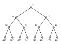
Figure 1. The infinite rooted regular binary tree ${\mathcal{T}}$.

By $\operatorname{Aut}({\mathcal{T}})$ we denote the group of automorphisms of ${\mathcal{T}}$. Any automorphism $\alpha\in\operatorname{Aut}({\mathcal{T}})$ can be viewed as a permutation on the set $\{0,1\}^{*}$ which preserves the length and initial segments, i.e., $|\alpha(x)|=|x|$ for all $x$ and if $\alpha(xy)=x^{\prime}y^{\prime}$ and $|x|=|x^{\prime}|$ then $\alpha(x)=x^{\prime}$. In particular, for every $n\geq 0$, $\alpha$ induces a permutation on the set $\{0,1\}^{n}$ of words of length  $n$ (the $n$-th level of ${\mathcal{T}}$). We denote by $\operatorname{St}(n)$ the stabilizer in $\operatorname{Aut}({\mathcal{T}})$ of the set $\{0,1\}^{n}$. In particular,

$$\operatorname{St}(1)=\{\alpha\in\operatorname{Aut}({\mathcal{T}})\mid\alpha(0)=0\text{ and }\alpha(1)=1\}$$

is the subgroup of $\operatorname{Aut}({\mathcal{T}})$ of index 2.

Let ${\mathcal{T}}_{0}$ and ${\mathcal{T}}_{1}$ be the subtrees of ${\mathcal{T}}$ spanned by the vertices starting with $0$ and $1$, respectively. By $a$ we denote the automorphism of ${\mathcal{T}}$ which swaps ${\mathcal{T}}_{0}$ and ${\mathcal{T}}_{1}$:

$$\alpha(xw)=\bar{x}w\quad\text{for}\quad x\in\{0,1\}$$

where $\bar{x}$ denotes $1-x$.

By definition, the Grigorchuk group $\Gamma$ is the subgroup of $Aut({\mathcal{T}})$ generated by four automorphisms $a,b,c$ and $d$, where $b,c,d\in\operatorname{St}(1)$ are defined recursively as follows:

$$b(0w) =0a(w), b(1w) =1c(w),$$

$$c(0w) =0a(w), c(1w) =1d(w),$$

$$d(0w) =0w, d(1w) =1b(w).$$

It is easy to see that the generators $a,b,c$ and $d$ satisfy the relations

(1) $$a^{2}=b^{2}=c^{2}=d^{2}=bcd=1.$$

In particular,

$$\langle a\rangle=\{1,a\}\simeq{\mathbb{Z}}/2{\mathbb{Z}}\quad\mbox{and}\quad\langle b,c,d\rangle=\{1,b,c,d\}\simeq{\mathbb{Z}}/2{\mathbb{Z}}\times{\mathbb{Z}}/2{\mathbb{Z}}.$$

Hence every element of $\Gamma$ can be represented by a word of the form

(2) $$[a]x_{1}ax_{2}a\ldots ax_{n}[a]$$

where $x_{i}\in\{b,c,d\}$ and the first and the last occurrences of $a$ are optional.

Every automorphism $g\in\operatorname{St}(1)$ induces automorphisms $g_{0}$ and $g_{1}$ on the subtrees ${\mathcal{T}}_{0}$ and  ${\mathcal{T}}_{1}$ of ${\mathcal{T}}$. Since ${\mathcal{T}}_{0}$ and ${\mathcal{T}}_{1}$ are naturally isomorphic to ${\mathcal{T}}$ the mapping $g\mapsto(g_{0},g_{1})$ gives a group isomorphism

$$\psi:\operatorname{St}(1)\rightarrow\operatorname{Aut}({\mathcal{T}})\times\operatorname{Aut}({\mathcal{T}}).$$

We denote by $\psi_{i}$ $(i=0,1)$ the components of $\psi$:

$$\psi(g)=(\psi_{0}(g),\ \psi_{1}(g)).$$

Observe that conjugation by $a$ swaps the components of $\psi(g)$:

$$\psi(aga)=(\psi_{1}(g),\ \psi_{0}(g)).$$

Let $St_{\Gamma}(1)=\operatorname{St}(1)\cap\Gamma$ be the set of automorphisms in $\Gamma$ stabilizing the first level of  ${\mathcal{T}}$, i.e., stabilizing the vertices 0 and 1. Since $b,c,d\in\operatorname{St}(1)$ and $a$ swaps ${\mathcal{T}}_{0}$ and ${\mathcal{T}}_{1}$, the subgroup $St_{\Gamma}(1)$ has index 2 in $\Gamma$ and a word $w$ represents an element of $St_{\Gamma}(1)$ if and only if $w$ has an even number of occurrences of $a^{\pm 1}$. This implies that $St_{\Gamma}(1)$ has a generating set $\{b,c,d,aba,aca,ada\}$. From the definition of $b$, $c$ and $d$ we can write immediately the images under $\psi$ of the generators of $St_{\Gamma}(1)$:

$$\psi(b) =(a,c), \psi(aba) =(c,a),$$

$$\psi(c) =(a,d), \psi(aca) =(d,a),$$

$$\psi(d) =(1,b), \psi(ada) =(b,1).$$

The monomorphism

$$\psi:St_{\Gamma}(1)\rightarrow\Gamma\times\Gamma$$

plays a central role in our analysis of equations in $\Gamma$. Note that computation of $\psi$ is effective (for example, we can represent an element of $St_{\Gamma}(1)$ by a reduced word (2) as a concatenation of generators $\{b,c,d,aba,aca,ada\}$ and then apply the formulas above).

We will need a description of the image of $\psi$ as well as an extra technical tool, the “subgroup $K$ trick” (Proposition 2.2) used in [13] for a solution of the conjugacy problem for $\Gamma$ (see also [9]). Let $K$ be the normal closure in $\Gamma$ of the element $abab$,

$$K=\langle abab\rangle^{\Gamma}.$$

Lemma 2.1.

The following holds:

1. $K$ has index $16$ in $\Gamma$ and the quotient group $\Gamma/K$ has the presentation

   $$\Gamma/K=\langle a,b,d\mid b^{2}=a^{2}=d^{2}=1,\ (ab)^{2}=(bd)^{2}=(ad)^{4}=1\rangle$$

2. $\Gamma/K$ is the direct product of the cyclic group of order 2 generated by $bK$ and the dihedral group of order 8 generated by $aK$ and $dK$.

3. $K\times K\subseteq\psi(K)$.

Proof.

(ii) follows from (i). (iii) is Proposition 30(v) in [6, Chapter VIII]. Proposition 30(ii) in [6, Chapter VIII] says that $K$ is of index 16. To verify the presentation for $\Gamma/K$ in (i) we first check that all defining relations hold in $\Gamma/K$ and then compute that the presented group is of order 16. ∎

By $\pi_{K}$ we denote the natural epimorphism $\Gamma\to\Gamma/K$. A straightforward consequence of Lemma  2.1(iii) is the following proposition.

Proposition 2.2.

There is a finite set ${\mathcal{F}}$ of pairs $(u,v)\in\Gamma/K\times\Gamma/K$ and a map $\omega:{\mathcal{F}}\to\Gamma/K$ such that:

1. A pair $(g_{0},g_{1})\in\Gamma\times\Gamma$ belongs to the image of $\psi$ if and only $(\pi_{K}(g_{0}),\pi_{K}(g_{1}))\in{\mathcal{F}}$.

2. If $(\pi_{K}(g_{0}),\pi_{K}(g_{1}))\in{\mathcal{F}}$ then for any $g\in\Gamma$ with $\psi(g)=(g_{0},g_{1})$, we have

   $$\pi_{K}(g)=\omega(\pi_{K}(g_{0}),\pi_{K}(g_{1})).$$

3. Quadratic equations

3.1. Equations in groups

Let $G$ be a group and $X$ a countable set of variables. An equation in $G$ is a formal equality $W=1$ where $W$ is a word $u_{1}u_{2}\dots u_{k}$ of letters $u_{i}\in G\cup X^{\pm 1}$. We view the left-hand side $W$ of an equation as an element of the free product $G*F_{X}$. A solution of $W=1$ is a homomorphism $\alpha:G*F_{X}\to G$ which is identical on $G$ (i.e. $\alpha$ is a $G$-homomorphism) and satisfies $\alpha(W)=1$. Similarly, a solution of a system of equations $\{W_{i}=1\}_{i\in I}$ is a $G$-homomorphism $\alpha:G*F_{X}\to G$ such that $\alpha(W_{i})=1$ for all $i$.

For the Diophantine problem in a group $G$, it is usually assumed that $G$ is finitely or countably generated; in this case equations in $G$ can be represented by words in a countable alphabet $A^{\pm 1}\cup X^{\pm 1}$ where $A$ is a generating set for $G$.

A word $W\in G\ast F_{X}$ and an equation $W=1$ are called quadratic if every variable $x\in X$ occurring in $W$ occurs exactly twice (where occurrences of both $x$ and $x^{-1}$ are counted). For a word $W\in G\ast F_{X}$ by $\operatorname{Var}(W)\subseteq X$ we denote the set of all variables occurring in $W$ (again, occurrences of $x^{\pm 1}$ are counted as occurrences of a variable $x$).

We denote $\operatorname{Aut^{f}}_{G}(G\ast F_{X})$ the group of finitely supported $G$-automorphisms of $G*F_{X}$, i.e., automorphisms $\phi\in\operatorname{Aut}(G\ast F_{X})$ which are identical on $G$ and change finitely many elements of $X$. We say that two words $V,W\in G*F_{X}$ are equivalent if there is an automorphism $\phi\in\operatorname{Aut^{f}}_{G}(G\ast F_{X})$ such that $\phi(V)$ is conjugate to  $W$. Clearly, if $V$ and $W$ are equivalent then equation $V=1$ has a solution if and only if equation $W=1$ has a solution.

It is well known that every quadratic word is equivalent to a word of one of the following forms:

(3) $$\begin{array}[]{c}[x_{1},y_{1}][x_{2},y_{2}]\ldots[x_{g},y_{g}]\qquad(g\geq 0),\\[2.15277pt] [x_{1},y_{1}][x_{2},y_{2}]\ldots[x_{g},y_{g}]\,c_{1}\,z_{2}^{-1}c_{2}z_{2}\dots z_{m}^{-1}c_{m}z_{m}\qquad(g\geq 0,\ m\geq 1),\\[2.15277pt] x_{1}^{2}x_{2}^{2}\ldots x_{g}^{2}\qquad(g>0),\\[2.15277pt] x_{1}^{2}x_{2}^{2}\ldots x_{g}^{2}\,c_{1}\,z_{2}^{-1}c_{2}z_{2}\dots z_{m}^{-1}c_{m}z_{m}\qquad(g>0,\ m\geq 1),\end{array}$$

where $x_{i},y_{i},z_{i}\in X$ are variables and $c_{i}\in G$ (see [2] or [5]). With a slight change of these canonical forms (introducing a new variable $z_{1}$, for technical convenience), we call the following quadratic words $Q$ and the corresponding quadratic equations $Q=1$ standard:

$$[x_{1},y_{1}][x_{2},y_{2}]\ldots[x_{g},y_{g}]\,z_{1}^{-1}c_{1}z_{1}\,z_{2}^{-1}c_{2}z_{2}\dots z_{m}^{-1}c_{m}z_{m}\qquad(g\geq 0,\ m\geq 0),$$

$$x_{1}^{2}x_{2}^{2}\ldots x_{g}^{2}\,z_{1}^{-1}c_{1}z_{1}\,z_{2}^{-1}c_{2}z_{2}\dots z_{m}^{-1}c_{m}z_{m}\qquad(g>0,\ m\geq 0).$$

Words in the first and in the second series are called standard orientable and standard non-orientable, respectively. More generally, a quadratic word $Q$ (and a quadratic equation $Q=1$) are called orientable if the two occurrences in $Q$ of each variable $x\in\operatorname{Var}(Q)$ have the opposite signs $x$ and $x^{-1}$ and non-orientable if there is a variable $x$ occurring in $Q$ twice with the same signs $x$ or $x^{-1}$.

The number $g$ is called the genus of a standard quadratic word $Q$. The elements $c_{1}$, $\dots$, $c_{m}$ of $G$ occurring in $Q$ are called the coefficients of $Q$.

Proposition 3.1.

Every quadratic word $Q$ is equivalent to a standard quadratic word $R$ which is orientable if and and only if $Q$ is orientable. Moreover, $R$ and the equivalence automorphism $\alpha\in\operatorname{Aut^{f}}_{G}(G*F_{X})$ that sends $Q$ to a conjugate of $R$ can be computed effectively for a given $Q$.

Proof.

Due to the reduction to the classical standard form (3) (the procedure in [2] or in  [5] is effective and preserves orientability), it is enough to prove that removal of the variable  $z_{1}$ in a standard quadratic word (in our sense) leads to an equivalent quadratic word. The following $G$-automorphism does the job:

$$[x_{1},y_{1}]\ldots[x_{g},y_{g}]\cdot z_{1}^{-1}c_{1}z_{1}\cdot\ldots\cdot z_{m}^{-1}c_{m}z_{m}\\ \xrightarrow{\phi}z_{1}^{-1}([x_{1},y_{1}]\ldots[x_{g},y_{g}]\cdot c_{1}z_{2}^{-1}c_{2}z_{2}\cdot\ldots\cdot z_{m}^{-1}c_{m}z_{m})z_{1}$$

where $\phi=(x_{i}\mapsto z_{1}^{-1}x_{i}z_{1},\ y_{i}\mapsto z_{1}^{-1}y_{i}z_{1},\ i=1,\dots,g,\ z_{i}\mapsto z_{i}z_{1},\ i=2,\dots,m).$ ∎

3.2. Equations with constraints modulo a subgroup

Let $H$ be a normal subgroup of a group  $G$. By $\pi_{H}$ we denote the canonical epimorphism $G\rightarrow G/H$.

Definition 3.2.

An equation in $G$ with a constraint modulo $H$ is a pair $(W=1,\gamma)$ where $W\in G\ast F_{X}$ and $\gamma$ is a map $\operatorname{Var}(W)\to G/H$. A solution of such an equation is a $G$-homomorphism $\alpha:G\ast F_{X}\to G$ satisfying $\alpha(W)=1$ and $\pi_{H}(\alpha(x))=\gamma(x)$ for every variable $x\in\operatorname{Var}(W)$.

This notion naturally extends to systems of equations in $G$. A constraint modulo $H$ for a system of equations $\{W_{i}=1\}$ is a map

$$\gamma:\bigcup_{i}\operatorname{Var}(W_{i})\to G/H.$$

A solution of a constrained system $(\{W_{i}=1\},\gamma)$ is a $G$-homomorphism $\alpha:G\ast F_{X}\to G$ such that $\alpha(W_{i})=1$ for all $i$ and $\pi_{H}(\alpha(x))=\gamma(x)$ for every $x\in\bigcup_{i}\operatorname{Var}(W_{i})$.

If $Y\subseteq X$ is a set of variables then a map $\gamma:Y\to G/H$ extends naturally to a group homomorphism $G*F_{Y}\to G/H$ by defining $\gamma(g)=\pi_{H}(g)$ for $g\in G$. We use the same notation $\gamma$ for this homomorphism (implicitly identifying the two maps). In particular, a constraint  $\gamma$ for a system of equations $\{R_{i}=1\}$ is identified with the induced homomorphism $G*F_{Y}\to G/H$ where $Y=\bigcup_{i}\operatorname{Var}(W_{i})$.

Observe that existence of a solution of a system of equations $(\{R_{i}=1\},\gamma)$ with a constraint  $\gamma$ automatically implies that $\gamma(R_{i})=1$ for all $i$.

We introduce equivalence of constrained equations in the following way.

Definition 3.3.

Equations $(W=1,\gamma)$ and $(V=1,\zeta)$ with constraints modulo $H$ are equivalent if $\gamma$ and $\zeta$ can be extended to homomorphisms $\bar{\gamma},\bar{\zeta}:G*F_{X}\to G/H$ so that for some $G$-automorphism $\phi\in\operatorname{Aut^{f}}_{G}(G*F_{X})$, $\phi(W)$ is conjugate to $V$ and $\bar{\zeta}=\bar{\gamma}\circ\phi$.

The following simple observation shows that a constraint is naturally induced by equivalence of equations.

Lemma 3.4.

Let $W$ and $V$ be equivalent words in $G*F_{X}$. Then for any constraint $\gamma:\operatorname{Var}(W)\to G/H$ there exists another constraint $\zeta:\operatorname{Var}(V)\to G/H$ such that equations $(W=1,\gamma)$ and $(V=1,\zeta)$ are equivalent. Given $W$, $\gamma$ and a $G$-automorphism $\phi\in\operatorname{Aut^{f}}_{G}(G*F_{X})$ sending $W$ to a conjugate of $V$, the constraint $\zeta$ can be effectively computed.

Proof.

To compute $\zeta$, we first extend $\gamma$ to a homomorphism $\bar{\gamma}:G*F_{X}\to G/H$ in an arbitrary way, then take $\bar{\zeta}=\bar{\gamma}\circ\phi$ and compute $\zeta$ by restricting $\bar{\zeta}$ to $F_{X}$. Since $\phi$ is finitely supported, the procedure is effective. ∎

As an immediate consequence of the lemma and Proposition 3.1 we get

Corollary 3.5.

For any quadratic equation $(Q=1,\gamma)$ with a constraint modulo $H$ there is an equivalent equation $(S=1,\zeta)$ where $S$ is a standard quadratic word equivalent to $Q$.

Assume that $W_{1}$ and $W_{2}$ are two words in $G\ast F_{X}$ and there is a variable $x\in X$ which occurs in each $W_{i}$ exactly once. Let

$$W_{i}=U_{i}x^{\varepsilon_{i}}V_{i}\quad\text{where $\varepsilon_{i}=\pm 1$}.$$

We can express  $x$ in  $W_{2}$ as $x=(V_{2}U_{2})^{-\varepsilon_{2}}$ and then substitute the expression in $W_{1}$ obtaining a new word denoted $W_{1}\#_{x}W_{2}$ in which $x$ no longer occurs:

$$W_{1}\#_{x}W_{2}=U_{1}(V_{2}U_{2})^{-\varepsilon_{1}\varepsilon_{2}}V_{1}.$$

Sometimes we simply write $W_{1}\#W_{2}$ if the choice of $x$ is irrelevant (see also Remark 3.7). It is obvious that a system $\{W_{1}=1,W_{2}=1\}$ is solvable in $G$ if and only if a single equation $W_{1}\#_{x}W_{2}=1$ is solvable in $G$. We will need a similar statement for the case of equations with constraints.

Lemma 3.6.

Let $W_{1},W_{2}\in G\ast F_{X}$ and assume that a variable $x\in X$ occurs in each  $W_{i}$ exactly once. Let $(\{W_{1}=1,W_{2}=1\},\gamma)$ be a system of equations in $G$ with a constraint $\gamma$ modulo  $H$ and $\gamma(W_{i})=1$ for $i=1,2$. Then this system has a solution if and only if the equation $(W_{1}\#_{x}W_{2}=1,\gamma^{\prime})$ has a solution where $\gamma^{\prime}$ is the restriction of $\gamma$ on $\operatorname{Var}(W_{1}\#_{x}W_{2})$.

Proof.

The “only if” part is obvious. For the “if” part, we use the condition $\gamma(W_{i})=1$ which implies that any solution $\alpha^{\prime}$ of the constrained equation $(W_{1}\#_{x}W_{2}=1,\ \gamma^{\prime})$ extends to a solution of the system $\{W_{1}=1,W_{2}=1\}$ with $\pi_{H}(\alpha(x))=\gamma(x)$. ∎

Remark 3.7.

It is easy to see that if $y$ is another variable which occurs in either $W_{1}$ and $W_{2}$ exactly once then $W_{1}\#_{y}W_{2}$ and $W_{1}\#_{x}W_{2}$ are equivalent. However, we do not need this fact and the notation $W_{1}\#W_{2}$ means a particular choice of a variable $x$ which is clear from the context.

4. Splitting equations

4.1. Splitting words in $\Gamma*F_{X}$

Let $W=1$ be an equation in $\Gamma$. If we substitute the values of a solution to $W$ and apply the splitting homomorphism $\psi$ then we get two new equalities. These equalities lead in a natural way to a system $\{W_{0}=1,\ W_{1}=1\}$ of two equations in  $\Gamma$ formally defined below in this section. The main idea of splitting an equation is that we get a new equivalent system which, in a certain sense, is simpler than the initial equation. Equivalence, however, cannot be achieved in a straightforward way. An obstruction appears because the image of  $\operatorname{St}_{\Gamma}(1)$ under $\psi$ is a proper subgroup of $\Gamma\times\Gamma$ and, in general, a solution of the system $\{W_{0}=1,W_{1}=1\}$ can not be lifted to a solution of $W=1$. This is the reason why we engage equations with constraints modulo  $K$: since we have $\psi(K)\supset K\times K$, for constrained equations the transition from $W=1$ to $\{W_{0}=1,\ W_{1}=1\}$ is equivalent (see Corollary 4.3).

Starting from this point, we consider only equations in $\Gamma$ with constraints modulo $K$ (often omitting mentioning the constraints). Since $K$ is a subgroup of $\Gamma$ of finite index, any equation in $\Gamma$ is reduced to a finite disjunction of equations with constraints modulo $K$.

On the set of words $W\in\Gamma*F_{X}$ we define two maps $\Psi_{0}$ and $\Psi_{1}$ which simulate application of the homomorphisms $\psi_{0}$ and $\psi_{1}$ after substituting values of the variables in $W$. Since $\psi$ is defined on the subgroup $\operatorname{St}_{\Gamma}(1)$ of $\Gamma$ of index  2, $\Psi_{0}(W)$ and $\Psi_{1}(W)$ depend on the predefined cosets modulo $\operatorname{St}_{\Gamma}(1)$ of all values of variables occurring in  $W$. We observe that a constraint modulo  $K$ determines these cosets in a unique way. For this reason, we formally define maps  $\Psi_{i}$ with respect to a given constraint $\gamma:\operatorname{Var}(W)\to\Gamma/K$ (though denoting them $\Psi_{i}$ by abuse of notations).

Given a constraint $\gamma:Y\to\Gamma/K$ on a set of variables $Y\subseteq X$, we use the notation $\sigma_{\gamma}$ for the induced group homomorphism

$$\sigma_{\gamma}:\Gamma*F_{Y}\to\Gamma/\operatorname{St}_{\Gamma}(1)$$

into the group $\Gamma/\operatorname{St}_{\Gamma}(1)$ of order 2 which gives the coset mod $\operatorname{St}_{\Gamma}(1)$ of every word $U\in\Gamma*F_{Y}$.

For an element $u\in\Gamma$, let $\bar{u}$ denote the closest element in $\operatorname{St}_{\Gamma}(1)$ defined by

$$\bar{u}=\begin{cases}u&\mbox{if }u\in\operatorname{St}_{\Gamma}(1),\\ ua&\mbox{otherwise.}\\ \end{cases}$$

For each variable $x\in X$ we introduce two variables $x_{0}$ and $x_{1}$ which we call the descendants of $x$. Since we operate on a single set of variables $X$ (and the splitting procedure will be applied to an equation recursively) we may formally assume that $X$ is partitioned into two infinite disjoint sets $X_{0}$ and $X_{1}$ and two bijections $X\to X_{0}$, $X\to X_{1}$ are fixed which provide the descendants of $x\in X$.

Now, given a word

$$W=u_{1}u_{2}\dots u_{k}\in\Gamma\ast F_{X},\quad u_{i}\in\Gamma\cup X^{\pm 1},$$

and a constraint $\gamma:\operatorname{Var}(W)\to\Gamma/K$ we define a word:

$$\Psi_{0}(W)=v_{1}v_{2}\dots v_{k}\in\Gamma*F_{X},$$

where for $u_{i}\in\Gamma$,

$$v_{i}=\begin{cases}\psi_{0}(\bar{u}_{i})&\text{if }\sigma_{\gamma}(u_{1}\dots u_{i-1})=1\\ \psi_{0}(a\bar{u}_{i}a)&\text{if }\sigma_{\gamma}(u_{1}\dots u_{i-1})\neq 1\\ \end{cases}$$

and for $u_{i}=x^{\varepsilon}\in X^{\pm 1}$,

$$v_{i}=\begin{cases}x_{0}&\text{if }\sigma_{\gamma}(u_{1}\dots u_{i-1})=1\\ x_{1}&\text{if }\sigma_{\gamma}(u_{1}\dots u_{i-1})\neq 1\\ \end{cases}\quad\text{for }\varepsilon=1,\qquad v_{i}=\begin{cases}x_{0}^{-1}&\text{if }\sigma_{\gamma}(u_{1}\dots u_{i})=1\\ x_{1}^{-1}&\text{if }\sigma_{\gamma}(u_{1}\dots u_{i})\neq 1\\ \end{cases}\quad\text{for }\varepsilon=-1.$$

Similarly one defines $\Psi_{1}(W)$ by taking $\psi_{1}$ instead of $\psi_{0}$ in the definition of $v_{i}$ for $u_{i}\in\Gamma$ and interchanging $x_{0}$ and $x_{1}$ in the definition of $v_{i}$ for $u_{i}\in X^{\pm 1}$. We denote also

$$\Psi(W)=(\Psi_{0}(W),\>\Psi_{1}(W)).$$

Note that in the definition of $\Psi_{i}(W)$ we do not assume that $\sigma_{\gamma}(W)=1$ (i.e. that $W$ defines an element in $\operatorname{St}_{\Gamma}(1)$ after substituting values for all variables) and thus $\Psi_{i}(W)$ is defined for any word $W\in\Gamma*F_{X}$. In particular, we have a function $\Psi:\Gamma*F(X)\rightarrow(\Gamma*F(X))\times(\Gamma*F(X))$. Note also that $\Psi_{i}(W)=\Psi_{i}(Wa)$ for any $W$, which can be seen directly from the definition.

Let $W\in\Gamma\ast F(X)$ and $\gamma:\operatorname{Var}(W)\to\Gamma/K$ be a constraint on $\operatorname{Var}(W)$ (remember that $\Psi(W)$ is formally defined with respect to a given $\gamma$). For any $\Gamma$-homomorphism $\alpha:\Gamma*F_{\operatorname{Var}(W)}\to\Gamma$ we can define the induced map $\alpha_{*}:\Gamma*F_{\operatorname{Var}(\Psi_{0}(W))\cup\operatorname{Var}(\Psi_{1}(W))}\to\Gamma$ by

$$\alpha_{*}(x_{i})=\psi_{i}(\overline{\alpha(x)})\qquad\text{for $x\in\operatorname{Var}(W)$ and $i=0,1$}.$$

The next proposition follows from the construction by induction on the length of $W$.

Proposition 4.1 (The main property of $\Psi$).

For any $\Gamma$-homomorphism $\alpha:\Gamma*F_{\operatorname{Var}(W)}\to\Gamma$ satisfying the constraint  $\gamma$ (that is, $\pi_{K}(\alpha(x))=\gamma(x)$ for any $x\in\operatorname{Var}(W)$) we have $\psi_{i}(\overline{\alpha(W)})=\alpha_{*}(\Psi_{i}(W))$ ($i=0,1$). ∎

We are in position to define splitting of an equation in $\Gamma$ with a constraint modulo  $K$. Since the images $\psi_{i}(gK)$ of a coset $gK$ do not belong to a unique coset modulo $K$, a constraint modulo $K$ generates a family of constraints under splitting. To define this family, we use a notation $\bar{g}$ for an element $g\in\Gamma/K$ which plays the role of “the closest element in the stabilizer $\operatorname{St}_{1}(\Gamma)$” (similar to the case of notation $\bar{g}$ for $g\in\Gamma$):

$$\bar{g}=\begin{cases}g&\text{if}\ g\in\operatorname{St}_{1}(\Gamma)/K,\\ g\,\pi_{K}(a)&\text{otherwise,}\end{cases}$$

where $\pi_{K}(a)$ denotes the natural image of $a$ in $\Gamma/K$.

Definition 4.2.

Given a word $W\in\Gamma*F_{X}$ and a map $\gamma:\operatorname{Var}(W)\to\Gamma/K$, we define a set ${\mathcal{V}}_{W,\gamma}$ of maps $\zeta:\operatorname{Var}(\Psi_{0}(W))\cup\operatorname{Var}(\Psi_{1}(W))\to\Gamma/K$:

(4) $${\mathcal{V}}_{W,\gamma}=\{\zeta\mid\omega(\zeta(x_{0}),\zeta(x_{1}))=\overline{\gamma(x)}\text{ for all $x\in\operatorname{Var}(W)$}\}$$

where $\omega$ is given in Proposition 2.2.

An immediate consequence of Propositions 4.1 and 2.2 is the following corollary.

Corollary 4.3 (The splitting reduction).

Let $(W=1,\gamma)$ be an equation in $\Gamma$ and $\sigma_{\gamma}(W)=1$. Then $(W=1,\gamma)$ is solvable if and only if the system $(\{\Psi_{0}(W)=1,\>\Psi_{1}(W)=1\},\ \zeta)$ is solvable for some $\zeta\in{\mathcal{V}}_{W,\gamma}$. ∎

4.2. Splitting quadratic equations

In this subsection, we apply $\Psi$ to standard quadratic equations in $\Gamma$.

It follows from the definition of $\Psi_{i}$ that for any $U,V\in\Gamma*F_{X}$:

$$\Psi_{i}(U\cdot V)=\begin{cases}\Psi_{i}(U)\cdot\Psi_{i}(V)&\text{if }\sigma_{\gamma}(U)=1,\\ \Psi_{i}(U)\cdot\Psi_{1-i}(V)&\text{if }\sigma_{\gamma}(U)\neq 1.\end{cases}$$

Hence the image of a standard quadratic word under $\Psi_{i}$ is factored into blocks of the form $\Psi_{i}([x,y])$, $\Psi_{i}(x^{2})$ and $\Psi_{j}(z^{-1}cz)$, $j=0,1$. (Note that $\sigma_{\gamma}([x,y])=\sigma_{\gamma}(x^{2})=1$.) We write explicit expressions for these factors (we assume that commutators $[x,y]$ are written as $x^{-1}y^{-1}xy$):

$$\Psi_{0}([x,y]) =x_{0}^{-1}y_{0}^{-1}x_{0}y_{0}, \Psi_{1}([x,y]) =x_{1}^{-1}y_{1}^{-1}x_{1}y_{1} \text{if }\sigma_{\gamma}(x)=\sigma_{\gamma}(y)=1,$$

$$\Psi_{0}([x,y]) =x_{1}^{-1}y_{1}^{-1}x_{1}y_{0}, \Psi_{1}([x,y]) =x_{0}^{-1}y_{0}^{-1}x_{0}y_{1} \text{if }\sigma_{\gamma}(x)\neq 1,\ \sigma_{\gamma}(y)=1,$$

$$\Psi_{0}([x,y]) =x_{0}^{-1}y_{1}^{-1}x_{1}y_{1}, \Psi_{1}([x,y]) =x_{1}^{-1}y_{0}^{-1}x_{0}y_{0} \text{if }\sigma_{\gamma}(x)=1,\ \sigma_{\gamma}(y)\neq 1,$$

$$\Psi_{0}([x,y]) =x_{1}^{-1}y_{0}^{-1}x_{0}y_{1}, \Psi_{1}([x,y]) =x_{0}^{-1}y_{1}^{-1}x_{1}y_{0} \text{if }\sigma_{\gamma}(x),\sigma_{\gamma}(y)\neq 1,$$

$$\Psi_{0}(x^{2}) =x_{0}^{2}, \Psi_{1}(x^{2}) =x_{1}^{2}, \text{if }\sigma_{\gamma}(x)=1,$$

$$\Psi_{0}(x^{2}) =x_{0}x_{1}, \Psi_{1}(x^{2}) =x_{1}x_{0}, \text{if }\sigma_{\gamma}(x)\neq 1,$$

and finally,

$$\Psi_{0}(z^{-1}cz) =z_{0}^{-1}c_{0}z_{0}, \Psi_{1}(z^{-1}cz) =z_{1}^{-1}c_{1}z_{1} \text{if }c\in St_{\Gamma}(1),\ \sigma_{\gamma}(z)=1,$$

$$\Psi_{0}(z^{-1}cz) =z_{0}^{-1}c_{0}z_{1}, \Psi_{1}(z^{-1}cz) =z_{1}^{-1}c_{1}z_{0} \text{if }c\notin St_{\Gamma}(1),\ \sigma_{\gamma}(z)=1,$$

$$\Psi_{0}(z^{-1}cz) =z_{1}^{-1}c_{1}z_{1}, \Psi_{1}(z^{-1}cz) =z_{0}^{-1}c_{0}z_{0} \text{if }c\in St_{\Gamma}(1),\ \sigma_{\gamma}(z)\neq 1,$$

$$\Psi_{0}(z^{-1}cz) =z_{1}^{-1}c_{1}z_{0}, \Psi_{1}(z^{-1}cz) =z_{0}^{-1}c_{0}z_{1} \text{if }c\notin St_{\Gamma}(1),\ \sigma_{\gamma}(z)\neq 1.$$

where

$$c_{i}=\psi_{i}(c),\quad i=0,1.$$

For a standard quadratic word $Q$, denote by $C(Q)$ the set of coefficients of $Q$.

Lemma 4.4.

Let $(Q=1,\gamma)$ be a standard quadratic equation in $\Gamma$ and $\Psi(Q)=(Q_{0},Q_{1})$. Then the following assertions are true.

1. $\operatorname{Var}(Q_{0})\cap\operatorname{Var}(Q_{1})=\emptyset$ if and only if $C(Q)\subseteq\operatorname{St}_{\Gamma}(1)$ and either $\sigma_{\gamma}(x_{i})=\sigma_{\gamma}(y_{i})=1$ for every commutator $[x_{i},y_{i}]$ in the commutator part of  $Q$ (if  $Q$ is standard orientable) or $\sigma_{\gamma}(x_{i})=1$ for every square $x_{i}^{2}$ in the square part of  $Q$ (if  $Q$ is standard non-orientable).

2. If $\operatorname{Var}(Q_{0})\cap\operatorname{Var}(Q_{1})=\emptyset$, then both $Q_{0}$ and $Q_{1}$ are standard quadratic words of the same genus $g$ and the same orientability as of $Q$. Furthermore,

   $$C(Q_{i})=\{\psi_{i}(c)\mid c\in C(Q),\ \psi_{i}(c)\neq 1\}.$$

3. If $x\in\operatorname{Var}(Q_{0})\cap\operatorname{Var}(Q_{1})$, then $Q_{0}\#_{x}Q_{1}$ is a quadratic word. If $Q$ is orientable then $Q_{0}\#_{x}Q_{1}$ is also orientable.

Proof.

Straightforward verification. ∎

In Lemma 4.5 we collect all necessary computations which we will use later to describe the standard form of the quadratic word $Q_{0}\#Q_{1}$ in the case $\operatorname{Var}(Q_{0})\cap\operatorname{Var}(Q_{1})\neq\emptyset$. We write $U\sim V$ for equivalence of words $U,V\in\Gamma*F_{X}$.

Lemma 4.5.

Let $Q$ be a quadratic word, $x_{0},x_{1},y_{0},y_{1},z_{1},z_{2},z_{3},z_{4}$ be variables not occurring in $Q$, and $c_{1},c_{2},c_{3},c_{4}\in\Gamma$. The following holds:

1. If $Q=UV$ then

   $$U[x_{0},y_{0}]V\sim[x_{0},y_{0}]Q,\quad Ux_{0}^{2}V\sim x_{0}^{2}Q\quad\text{and}\quad Uz_{1}^{-1}c_{1}z_{1}V\sim Qz_{1}^{-1}c_{1}z_{1}.$$

2. If $Q=UVW$ and $(R,S)$ is one of the pairs

   $$(x_{1}^{-1}y_{1}^{-1}x_{1}y_{0},\ x_{0}^{-1}y_{0}^{-1}x_{0}y_{1}),\quad(x_{0}^{-1}y_{1}^{-1}x_{1}y_{1},\ x_{1}^{-1}y_{0}^{-1}x_{0}y_{0})\quad\text{or}\quad(x_{1}^{-1}y_{0}^{-1}x_{0}y_{1},\ x_{0}^{-1}y_{1}^{-1}x_{1}y_{0})$$

   then

   $$URVSW\sim[x_{0},y_{0}][x_{1},y_{1}]Q.$$

3. If $Q=UVW$ then $Ux_{0}x_{1}Vx_{1}x_{0}W\sim x_{0}^{2}x_{1}^{2}Q.$

4. If $Q=UVW$ then

   $$U\cdot z_{1}^{-1}c_{1}z_{2}\cdot z_{3}^{-1}c_{3}z_{4}\cdot V\cdot z_{2}^{-1}c_{2}z_{1}\cdot z_{4}^{-1}c_{4}z_{3}\cdot W\sim[x_{0},y_{0}]Q\cdot z_{1}^{-1}c_{1}c_{2}z_{1}\cdot z_{2}^{-1}c_{3}c_{4}z_{2}.$$

5. If $(R,S)$ is one of the pairs in (ii), then $R\#S\sim[x_{0},x_{1}]$.

6. $z_{1}^{-1}c_{1}z_{2}\cdot z_{3}^{-1}c_{3}z_{4}\>\#\>z_{2}^{-1}c_{2}z_{1}\cdot z_{4}^{-1}c_{4}z_{3}\sim z_{1}^{-1}c_{1}c_{2}z_{1}\cdot z_{2}^{-1}c_{3}c_{4}z_{2}.$

Proof.

Straightforward computations. (i):

$$U[x_{0},y_{0}]V\xrightarrow{(x_{0}\mapsto U^{-1}x_{0}U,\ y_{0}\mapsto U^{-1}y_{0}U)}[x_{0},y_{0}]UV,$$

$$Ux_{0}^{2}V\xrightarrow{(x_{0}\mapsto U^{-1}x_{0}U)}x_{0}^{2}UV,$$

$$Uz_{1}^{-1}c_{1}z_{1}V\xrightarrow{(z_{1}\mapsto z_{1}V^{-1})}UVz_{1}^{-1}c_{1}z_{1}.$$

To prove (ii), assume $R=x_{1}^{-1}y_{1}^{-1}x_{1}y_{0}$ and $S=x_{0}^{-1}y_{0}^{-1}x_{0}y_{1}$. Then:

$$Ux_{1}^{-1}y_{1}^{-1}x_{1}y_{0}Vx_{0}^{-1}y_{0}^{-1}x_{0}y_{1}W \xrightarrow{(x_{0}\mapsto x_{0}V,\ x_{1}\mapsto V^{-1}x_{1},\ y_{1}\mapsto V^{-1}y_{1}V)}\quad Ux_{1}^{-1}y_{1}^{-1}x_{1}y_{0}x_{0}^{-1}y_{0}^{-1}x_{0}y_{1}VW$$

$$\xrightarrow{(x_{i}\mapsto U^{-1}x_{i}U,\ y_{i}\mapsto U^{-1}y_{i}U),\ i=0,1}\quad x_{1}^{-1}y_{1}^{-1}x_{1}y_{0}x_{0}^{-1}y_{0}^{-1}x_{0}y_{1}UVW$$

$$\xrightarrow{(x_{0}\mapsto y_{1}x_{0}y_{1}^{-1},\ y_{0}\mapsto y_{1}y_{0}y_{1}^{-1})}\quad [x_{0},y_{1}][y_{0}^{-1},x_{1}]UVW$$

$$\sim\quad [x_{0},y_{0}][x_{1},y_{1}]UVW.$$

The other two cases for $(R,S)$ are similar.

(iii): The quadratic word $Ux_{0}x_{1}Vx_{1}x_{0}W$ can be modified as follows:

$$Ux_{0}x_{1}Vx_{1}x_{0}W\xrightarrow{(x_{0}\mapsto x_{0}V,\ x_{1}\mapsto V^{-1}x_{1})}\quad Ux_{0}x_{1}^{2}x_{0}VW$$

$$\xrightarrow{(x_{0}\mapsto U^{-1}x_{0}U,\ x_{1}\mapsto Ux_{1}U^{-1})}\quad x_{0}x_{1}^{2}x_{0}UVW$$

$$\xrightarrow{(x_{0}\mapsto x_{0}x_{1}^{-2},\ x_{1}\mapsto x_{1}^{-1})}\quad x_{0}^{2}x_{1}^{2}UVW.$$

(iv): The quadratic word $Uz_{1}^{-1}c_{1}z_{2}z_{3}^{-1}c_{3}z_{4}Vz_{2}^{-1}c_{2}z_{1}z_{4}^{-1}c_{4}z_{3}W$ can be modified as follows:

$$Uz_{1}^{-1}c_{1}z_{2}z_{3}^{-1}c_{3}z_{4}Vz_{2}^{-1}c_{2}z_{1}z_{4}^{-1}c_{4}z_{3}W$$

$$\xrightarrow{(z_{2}\mapsto z_{2}V,\ z_{3}\mapsto z_{3}V)} Uz_{1}^{-1}c_{1}z_{2}z_{3}^{-1}c_{3}z_{4}z_{2}^{-1}c_{2}z_{1}z_{4}^{-1}c_{4}z_{3}VW$$

$$\xrightarrow{(z_{1}\mapsto z_{1}U,\ z_{4}\mapsto z_{4}U)} z_{1}^{-1}c_{1}z_{2}z_{3}^{-1}c_{3}z_{4}Uz_{2}^{-1}c_{2}z_{1}z_{4}^{-1}c_{4}z_{3}VW$$

$$\xrightarrow{(z_{2}\mapsto z_{2}U,\ z_{3}\mapsto z_{3}U)} z_{1}^{-1}c_{1}z_{2}z_{3}^{-1}c_{3}z_{4}z_{2}^{-1}c_{2}z_{1}z_{4}^{-1}c_{4}z_{3}UVW$$

A reduction of $z_{1}^{-1}c_{1}z_{2}z_{3}^{-1}c_{3}z_{4}z_{2}^{-1}c_{2}z_{1}z_{4}^{-1}c_{4}z_{3}$ to the standard form gives

$$z_{1}^{-1}c_{1}z_{2}z_{3}^{-1}c_{3}z_{4}z_{2}^{-1}c_{2}z_{1}z_{4}^{-1}c_{4}z_{3}Q\sim[x_{0},y_{0}]z_{1}^{-1}c_{1}c_{2}z_{1}z_{2}^{-1}c_{3}c_{4}z_{2}Q.$$

We then move the factor $z_{1}^{-1}c_{1}c_{2}z_{1}z_{2}^{-1}c_{3}c_{4}z_{2}$ to the end of $Q$ by (i). Equivalences (v) and (vi) are similar. ∎

Proposition 4.6 (Non-disjoint orientable case).

Let $(Q=1,\gamma)$ be a quadratic equation where

$$Q=[x_{1},y_{1}][x_{2},y_{2}]\ldots[x_{g},y_{g}]\cdot z_{1}^{-1}c_{1}z_{1}\cdot\ldots\cdot z_{m}^{-1}c_{m}z_{m}$$

is a standard orientable quadratic word and $\sigma_{\gamma}(Q)=1$. Let $\Psi(Q)=(Q_{0},Q_{1})$. Assume that $\operatorname{Var}(Q_{0})\cap\operatorname{Var}(Q_{1})\neq\emptyset$. Then $Q_{0}\#Q_{1}$ is equivalent to a standard quadratic word:

$$R=[x_{1},y_{1}][x_{2},y_{2}]\ldots[x_{h},y_{h}]\cdot z_{1}^{-1}d_{1}z_{1}\cdot\ldots\cdot z_{l}^{-1}d_{l}z_{l}$$

satisfying the following:

1. $h=2g+\frac{1}{2}\delta(Q)-1$, where $\delta(Q)$ is the cardinality of the set $\{i\mid c_{i}\notin\operatorname{St}_{\Gamma}(1)\}$;

2. $C(R)=\cup_{i=1}^{m}K_{i}\setminus\{1\}$, where

   $$K_{i}=\begin{cases}\{\psi_{0}(c_{i}),\>\psi_{1}(c_{i})\}&\text{if }c_{i}\in\operatorname{St}_{\Gamma}(1),\\ \{\psi_{0}(c_{i}a)\psi_{1}(c_{i}a),\>\psi_{1}(c_{i}a)\psi_{0}(c_{i}a)\}&\text{if }c_{i}\notin\operatorname{St}_{\Gamma}(1).\end{cases}$$

Proof.

The assumption $\gamma(Q)\in\operatorname{St}_{\Gamma}(1)$ implies that the number $\delta(Q)$ is even. By Lemma 4.4(i), we have $\sigma_{\gamma}(x_{i})\neq 1$ or $\sigma_{\gamma}(y_{i})\neq 1$ for some commutator $[x_{i},y_{i}]$ in  $Q$ or $c_{j}\notin St_{\Gamma}(1)$ for some $j$. We compute the standard form of $Q_{0}\#Q_{1}$.

Case 1: $\sigma_{\gamma}(x_{i})\neq 1$ or $\sigma_{\gamma}(y_{i})\neq 1$ for some $i$. Let $Q=U[x_{i},y_{i}]V$. Then

$$Q_{0} =U_{0}x_{i1}^{-1}y_{i1}^{-1}x_{i1}y_{i0}V_{0}, Q_{1} =U_{1}x_{i0}^{-1}y_{i0}^{-1}x_{i0}y_{i1}V_{1} \text{if }\sigma_{\gamma}(x_{i})\neq 1,\ \sigma_{\gamma}(y_{i})=1,$$

$$Q_{0} =U_{0}x_{i0}^{-1}y_{i1}^{-1}x_{i1}y_{i1}V_{0}, Q_{1} =U_{1}x_{i1}^{-1}y_{i0}^{-1}x_{i0}y_{i0}V_{1} \text{if }\sigma_{\gamma}(x_{i})\neq 1,\ \sigma_{\gamma}(y_{i})=1,$$

$$Q_{0} =U_{0}x_{i1}^{-1}y_{i0}^{-1}x_{i0}y_{i1}V_{0}, Q_{1} =U_{1}x_{i0}^{-1}y_{i1}^{-1}x_{i1}y_{i0}V_{1} \text{if }\sigma_{\gamma}(x_{i})\neq 1,\ \sigma_{\gamma}(y_{i})=1$$

where $U_{k}=\Psi_{k}(U)$, $V_{k}=\Psi_{k}(V)$ for $k=0,1$. We have the corresponding cases for $Q_{0}\#Q_{1}$:

$$Q_{0}\#_{y_{i0}}Q_{1} =U_{0}x_{i1}^{-1}y_{i1}^{-1}x_{i1}x_{i0}y_{i1}V_{1}U_{1}x_{i0}^{-1}V_{0},\quad\text{or}$$

$$Q_{0}\#_{x_{i1}}Q_{1} =U_{0}x_{i0}^{-1}y_{i1}^{-1}y_{i0}^{-1}x_{i0}y_{i0}V_{1}U_{1}y_{i1}V_{0},\quad\text{or}$$

$$Q_{0}\#_{x_{i0}}Q_{1} =U_{0}x_{i1}^{-1}y_{i0}^{-1}y_{i1}^{-1}x_{i1}y_{i0}V_{1}U_{1}y_{i1}V_{0}.$$

Assume that $\sigma_{\gamma}(x_{i})\neq 1$ and $\sigma_{\gamma}(y_{i})=1$ (the other two cases are similar). Using Lemma 4.5 we reduce $Q_{0}\#_{y_{i0}}Q_{1}$ to a standard form $R$:

• By statements (i) and (ii) of the lemma, collect words $\psi_{k}([x_{j},y_{j}])$ for each commutator $[x_{j},y_{j}]$ in $UV$ to the left; each commutator $[x_{j},y_{j}]$ in $UV$ contributes then two commutators to $R$.

• By statement (i) of the lemma, collect words $\psi_{k}(z_{j}^{-1}c_{j}z_{j})$ for each coefficient factor $z_{j}^{-1}c_{j}z_{j}$ with $c_{j}\in\operatorname{St}_{\Gamma}(1)$ to the right; each factor $z_{j}^{-1}c_{j}z_{j}$ contributes to $R$ at most two coefficient factors of a similar form (if $\psi_{k}(c_{j})=1$ then the factor with $\psi_{k}(c_{j})$ disappears).

• By statement (vi) of the lemma, collect words $\psi_{k}(z_{j}^{-1}c_{j}z_{j})$ for the remaining coefficient factors $z_{j}^{-1}c_{j}z_{j}$ with $c_{j}\notin\operatorname{St}_{\Gamma}(1)$ to the right (they are now paired as in the left-hand side of the equivalence in (vi)). Each pair of factors $z_{j}^{-1}c_{j}z_{j}$ with $c_{j}\notin\operatorname{St}_{\Gamma}(1)$ contributes one commutator and at most one coefficient factor to $R$;

• Finally, replace the remaining non-reduced subword with a commutator by Lemma 4.5(v).

Case 2: $c_{j}\notin St_{\Gamma}(1)$ for some $j$. Let $Q=Uz_{j}^{-1}c_{j}z_{j}V$. Then

$$Q_{0}=U_{0}z_{j0}^{-1}c_{j0}z_{j1}V_{1},\quad Q_{1}=U_{1}z_{j1}^{-1}c_{j1}z_{j0}V_{0}\quad\text{if }\sigma_{\gamma}(z_{j})=1$$

$$Q_{0}=U_{0}z_{j1}^{-1}c_{j1}z_{j0}V_{1},\quad Q_{1}=U_{1}z_{j0}^{-1}c_{j0}z_{j1}V_{0}\quad\text{if }\sigma_{\gamma}(z_{j})\neq 1$$

where $U_{k}=\Psi_{k}(U)$, $V_{k}=\Psi_{k}(V)$, $c_{jk}=\psi_{k}(\bar{c}_{j})$, $k=0,1$. Up to re-enumeration of variables and coefficients, we may assume that $\sigma_{\gamma}(z_{j})=1$. In this case

$$Q_{0}\#_{z_{j0}}Q_{1}=U_{0}V_{0}U_{1}z_{j1}^{-1}c_{j1}c_{j0}z_{j1}V_{1}.$$

Then we proceed similarly to Case 1.

Statements (i) and (ii) of Proposition 4.6 now easily follow from the reduction process and right hand sides of the equivalences in Lemma 4.5(i,iv,vi). ∎

Proposition 4.7 (Non-disjoint non-orientable case).

Let $(Q=1,\gamma)$ be a quadratic equation where

$$Q=x_{1}^{2}x_{2}^{2}\ldots x_{g}^{2}\cdot z_{1}^{-1}c_{1}z_{1}\cdot\ldots\cdot z_{m}^{-1}c_{m}z_{m}$$

is a standard non-orientable quadratic word and $\sigma_{\gamma}(Q)=1$. Let $\Psi(Q)=(Q_{0},Q_{1})$ and $\operatorname{Var}(Q_{0})\cap\operatorname{Var}(Q_{1})\neq\emptyset$. Then $Q_{0}\#Q_{1}$ is equivalent to a standard quadratic word (which is non-orientable if $g>0$ and orientable otherwise)

$$R=x_{1}^{2}x_{2}^{2}\ldots x_{h}^{2}\cdot z_{1}^{-1}d_{1}z_{1}\cdot\ldots\cdot z_{l}^{-1}d_{l}z_{l}$$

satisfying the following:

1. $h=2g+\delta(Q)-2$;

2. $C(R)=\{d_{1},d_{2},\dots,d_{l}\}$ is the same as in Proposition  4.6.

Proof.

Similar to the proof of Proposition 4.6. There is a slight difference in computing the genus $h$: in case of a single square $Q=x_{0}^{2}$ we get:

$$R=x_{0}x_{1}\#x_{1}x_{0}=1$$

and each commutator coming from the coefficients by Lemma 4.5(iv) contributes $2$ to  $h$ by the equivalence $x^{2}[y,z]\sim z^{2}y^{2}z^{2}$. ∎

We summarize properties of the splitting operation for constrained quadratic equations in  $\Gamma$ in the following proposition.

Proposition 4.8.

Let $(Q=1,\gamma)$ be a standard quadratic equation in $\Gamma$ with a constraint modulo $K$. Assume that $\sigma_{\gamma}(Q)=1$ and let $\Psi(Q)=(Q_{0},Q_{1})$.

1. Suppose that $\operatorname{Var}(Q_{0})\cap\operatorname{Var}(Q_{1})=\emptyset$. Then $Q_{0}$ and $Q_{1}$ are standard quadratic words of the same genus and orientability as $Q$. The coefficients of  $Q_{i}$ are nontrivial elements $\psi_{i}(c_{j})$, where $c_{1},\dots,c_{m}$ are the coefficients of $Q$. There are finitely many pairs of constraints $(\gamma_{0j},\gamma_{1j})$ such that the equation $(Q=1,\gamma)$ is solvable if and only if, for some $j$, both equations $(Q_{0}=1,\gamma_{0j})$ and $(Q_{1}=1,\gamma_{1j})$ are solvable.

   The set $\{(\gamma_{0j},\gamma_{1j})\}$ of pairs of constraints $\gamma_{ij}$ is defined by restricting each constraint in ${\mathcal{V}}_{Q,\gamma}$ (see Definition 4.2) to $\operatorname{Var}(Q_{0})$ and $\operatorname{Var}(Q_{1})$. In other words, a pair $(\gamma_{0},\gamma_{1})$ belongs to this set if and only if

   $$\omega(\gamma_{0}(x_{0}),\gamma_{1}(x_{1}))=\overline{\gamma(x)}\quad\text{for each }x\in\operatorname{Var}(Q),$$

   where $x_{0},x_{1}$ are the descendants of a variable $x$ and $\omega$ is given by Proposition  2.2.

2. Suppose that $\operatorname{Var}(Q_{1})\cap\operatorname{Var}(Q_{2})\neq\emptyset$. Then there is a standard quadratic word  $R$ equivalent to $Q_{0}\#Q_{1}$ and finitely many constraints $\delta_{j}:\operatorname{Var}(R)\to\Gamma/K$ such that the equation $(Q=1,\gamma)$ is solvable if and only if, for some $j$, the equation $(R=1,\delta_{j})$ is solvable. If $Q$ is orientable then $R$ is orientable. The genus and the coefficients of  $R$ are as in Propositions  4.6 and  4.7.

   The set $\{\delta_{j}\}$ is defined in the following way. Let $\phi\in\operatorname{Aut^{f}}_{\Gamma}(\Gamma*F_{X})$ be a $\Gamma$-automorphism sending $Q_{0}\#Q_{1}$ to a conjugate of $R$. We take the set ${\mathcal{V}}_{Q,\gamma}$ of constraints for $Q_{0}\#Q_{1}$ defined in (4), and the subset ${\mathcal{U}}$ of ${\mathcal{V}}_{Q,\gamma}$ of those $\zeta\in{\mathcal{V}}_{Q,\gamma}$ which satisfy $\zeta(Q_{0})=\zeta(Q_{1})=1$. Then for each $\zeta\in{\mathcal{U}}$, we take its restriction on $\operatorname{Var}(Q_{0})\cup\operatorname{Var}(Q_{1})$ and produce a constraint $\delta:\operatorname{Var}(R)\to G/K$ using  $\phi$ by Lemma  3.4.

All the data provided by assertions (i) and (ii) can be effectively computed from the equation $(Q=1,\gamma)$.

Proof.

Follows from Lemmas 3.6, 4.4, Corollaries 3.5, 4.3 and Propositions 4.6, 4.7. ∎

Remark 4.9.

The transformation automorphism $\phi$ in Proposition 4.8(ii) that sends $Q_{0}\#Q_{1}$ to its standard form $R$ can be chosen in such a way that $\phi(Q_{0}\#Q_{1})=R$ without conjugation. This can be seen in a straightforward way from the proofs of Propositions 4.6 and 4.7 and the fact that conjugation in not needed in equivalences (v) and (vi) of Lemma 4.5.

5. Solution of the Diophantine problem for quadratic equations

In this section we prove Theorem 1 by presenting an algorithm which for a given (unconstrained) quadratic equation $Q=1$ in $\Gamma$ determines if the equation has a solution. The algorithm consists of Steps  1–5 below. To simplify notations, we assume that $Q$ is an orientable quadratic word (the non-orientable case is literally the same, with commutators replaced by squares).

Step 1. We reduce $Q$ to the standard form according to Proposition 3.1. Thus, from now on we write $Q$ as

$$Q=[x_{1},y_{1}]\ldots[x_{g},y_{g}]z_{1}^{-1}c_{1}z_{1}\ldots z_{m}^{-1}c_{m}z_{m}.$$

Step 2. We reduce the problem to constrained equations. For a given $Q$, we write a finite list of all possible constraints $\gamma_{i}:\operatorname{Var}(Q)\to\Gamma/K$. Then the equation $Q=1$ is solvable if and only if the constrained equation $(Q=1,\gamma_{i})$ is solvable for some $i$.

We assume now that we are given a constrained standard quadratic equation $(Q=1,\gamma)$.

Step 3. Given a standard equation $(Q=1,\gamma)$, we start recursive application of the splitting procedure described in Proposition 4.8. We use the following fact.

Proposition 5.1 (Coefficient reduction).

Let $(g_{0},g_{1},\dots)$ be a sequence of elements in $\Gamma$ satisfying the following condition

$$g_{i+1}\in\begin{cases}\{\psi_{0}(g_{i}),\>\psi_{1}(g_{i})\}&\mbox{ if }g_{i}\in\operatorname{St}_{\Gamma}(1)\\ \{\psi_{0}(g_{i}a)\psi_{1}(g_{i}a),\>\psi_{1}(g_{i}a)\psi_{0}(g_{i}a)\}&\mbox{ if }g_{i}\notin\operatorname{St}_{\Gamma}(1)\\ \end{cases}$$

Then there exists $M=M(g_{0})$ such that $|g_{n}|\leq 3$ for every $n\geq M$. In fact, one can take:

$$M=200+\log_{1.22}\max\{1,|g_{0}|-200\}.$$

Proof.

Follows from Proposition 3.6 in [9]. ∎

After applying the splitting operation at most $M$ times, we find a finite set ${\mathcal{F}}$ of systems of equations such that the solvability of $(Q=1,\gamma)$ is equivalent to the solvability of at least one system in ${\mathcal{F}}$. Each system in ${\mathcal{F}}$ is a finite set $\{(Q_{i}=1,\gamma_{i})\}$ of mutually independent quadratic equations $(Q_{i}=1,\gamma_{i})$ written in the standard form where the length of each coefficient is at most 3. Define a set:

$${\mathcal{S}}=\{g\in\Gamma\mid|g|\leq 3\}.$$

Denote by ${\mathcal{E}}_{\mathcal{S}}$ the set of all standard orientable quadratic equations $(Q=1,\gamma)$ with coefficients in ${\mathcal{S}}$. Now we may assume that we are given an equation $(Q=1,\gamma)$ in ${\mathcal{E}}_{\mathcal{S}}$.

Step 4. We fix a linear ordering on finite sets $\Gamma/K$ and ${\mathcal{S}}$. Given an equation $(Q=1,\gamma)$ in ${\mathcal{E}}_{\mathcal{S}}$, we transform it to the ordered form according to the following lemma:

Lemma 5.2 (Ordering factors).

For every equation $(Q=1,\gamma)$ in ${\mathcal{E}}_{\mathcal{S}}$, there exists (and can be effectively computed) an equivalent equation $(Q=1,\zeta)$ satisfying:

(5) $$(\zeta(x_{1}),\zeta(y_{1}))\preceq(\zeta(x_{2}),\zeta(y_{2}))\preceq\ldots\preceq(\zeta(x_{g}),\zeta(y_{g}))$$

and

(6) $$(c_{1},\zeta(z_{1}))\preceq(c_{2},\zeta(z_{2}))\preceq\ldots\preceq(c_{m},\zeta(z_{m}))$$

where “$\preceq$” is the lexicographic order induced by the orderings on $\Gamma/K$ and  ${\mathcal{S}}$.

Proof.

If $(\gamma(x_{i+1}),\gamma(y_{i+1}))\prec(\gamma(x_{i}),\gamma(y_{i}))$ then applying to $Q$ an automorphism:

$$(x_{i}\to[x_{i+1},y_{i+1}]x_{i}[x_{i+1},y_{i+1}]^{-1},\quad y_{i}\to[x_{i+1},y_{i+1}]y_{i}[x_{i+1},y_{i+1}]^{-1})$$

swaps $[x_{i},y_{i}]$ and $[x_{i+1},y_{i+1}]$ and, possibly, changes $\gamma(x_{i})$ and $\gamma(y_{i})$. For the new equation, the sequence of pairs

$$\bigl{(}(\gamma(x_{1}),\gamma(y_{1})),\ (\gamma(x_{2}),\gamma(y_{2})),\ \dots,\ (\gamma(x_{g}),\gamma(y_{g}))\bigr{)}$$

is lexicographically smaller than that for $Q$. Therefore, after applying a finite sequence of such automorphisms we get an equation satisfying (5).

If $(c_{i+1},\gamma(z_{i+1}))\prec(c_{i},\gamma(z_{i}))$, then applying to $Q$ an automorphism

$$(z_{i}\to z_{i}\cdot z_{i+1}^{-1}c_{i+1}^{-1}z_{i+1})$$

swaps $z_{i}^{-1}c_{i}^{-1}z_{i}$ and $z_{i+1}^{-1}c_{i+1}^{-1}z_{i+1}$ and, possibly, changes $\gamma(z_{i})$. For the new equation, the sequence of pairs

$$\bigl{(}(c_{1},\gamma(z_{1})),\ (c_{2},\gamma(z_{2})),\ \dots,\ (c_{m},\gamma(z_{m}))\bigr{)}$$

is lexicographically smaller than that for $Q$. Therefore, a sequence of such transformations stops in finitely many steps with an equation satisfying also (6). ∎

Step 5. Denote

$${\mathcal{B}}=(\Gamma/K\times\Gamma/K)\cup(\Gamma/K\times{\mathcal{S}}).$$

Note that ${\mathcal{B}}$ is finite since both $\Gamma/K$ and ${\mathcal{S}}$ are finite. Every ordered equation $(Q=1,\gamma)$ in  ${\mathcal{E}}_{\mathcal{S}}$ can be encoded as a function $\lambda_{Q,\gamma}\in{\mathbb{N}}^{\mathcal{B}}$ which associates

• to every pair $(g,h)\in\Gamma/K\times\Gamma/K$ the number of factors $[x_{i},y_{i}]$ in $Q$ such that $\gamma(x_{i})=g$ and $\gamma(y_{i})=h$;

• to every pair $(g,c)\in\Gamma/K\times{\mathcal{S}}$ the number of factors $z_{i}^{-1}c_{i}z_{i}$ in $Q$ such that $\gamma(z_{i})=g$ and $c_{i}=c$.

Let ${\mathcal{P}}$ be a set of all functions $\lambda_{Q,\gamma}$ encoding equations $(Q=1,\gamma)$ that have solutions. All we need to show is that ${\mathcal{P}}$ is recursive.

We fix any set of representatives in $\Gamma$ of all elements of $\Gamma/K$, so for any $h\in\Gamma/K$ we have $\hat{h}\in\Gamma$ with $\pi_{K}(\hat{h})=h$. Denote by $\mathit{Order}(g)$ the order of an element $g\in\Gamma$ (it is finite since $\Gamma$ is a 2-group, see Theorem 17 in [6, Chapter VIII]).

Let ${\mathcal{L}}\subseteq{\mathbb{N}}^{\mathcal{B}}$ be the set of all non-negative linear combinations of the following functions $\mu_{g,h}$ and $\nu_{g,c}$ where $(g,h)$ and $(g,c)$ run over $\Gamma/K\times\Gamma/K$ and $\Gamma/K\times{\mathcal{S}}$ respectively:

$$\mu_{g,h}\bigl{(}(g,h)\bigr{)}=\mathit{Order}([\hat{g},\hat{h}]),\quad\mu(u)=0\quad\text{for all other }u\in{\mathcal{B}}$$

and

$$\nu_{g,c}\bigl{(}(g,c)\bigr{)}=\mathit{Order}(c),\quad\mu(u)=0\quad\text{for all other }u\in{\mathcal{B}}.$$

Lemma 5.3.

${\mathcal{P}}+{\mathcal{L}}\subseteq{\mathcal{P}}$.

Proof.

It is enough to prove that ${\mathcal{P}}+\xi\subseteq{\mathcal{P}}$ where $\xi$ is either $\mu_{g,h}$ or $\nu_{g,c}$. Let $(Q=1,\gamma)$ and $(Q_{1}=1,\gamma_{1})$ be two equations such that $\lambda_{Q_{1},\gamma_{1}}=\lambda_{Q,\gamma}+\mu_{g,h}$. Then $Q_{1}$ is obtained from  $Q$ by inserting (at an appropriate place) the product $[x_{1},y_{1}]\dots[x_{r},y_{r}]$ of $r=\textit{Order}(\hat{g},\hat{h})$ commutators $[x_{i},y_{i}]$ and defining the constraint  $\gamma_{1}$ on the new variables by

$$\gamma_{1}(x_{1})=\gamma_{1}(x_{2})=\dots=\gamma_{1}(x_{r})=g\quad\text{and}\quad\gamma_{1}(y_{1})=\gamma_{1}(y_{2})=\dots=\gamma_{1}(y_{r})=h.$$

If $\alpha$ is a solution of $(Q=1,\gamma)$ then we can define a solution $\alpha_{1}$ of $(Q_{1}=1,\gamma_{1})$ by extending  $\alpha$ on the new variables $\{x_{i},y_{i}\}$ by setting $\alpha_{1}(x_{i})=\hat{g}$ and $\alpha_{1}(y_{i})=\hat{h}$ for all $i$. The case when $\xi=\nu_{g,c}$ is similar. ∎

Lemma 5.4.

Let $R$ be a subset of ${\mathbb{N}}^{n}$ such that $R+{\mathbb{N}}^{n}\subseteq R$. Then there exist finitely many vectors $v_{1},\ldots,v_{m}\in R$ such that

$$R=(v_{1}+{\mathbb{N}}^{n})\cup\ldots\cup(v_{m}+{\mathbb{N}}^{n}).$$

Proof.

We proceed by induction on $n$. For $n=1$ the statement is obvious. Assume that the lemma is true in dimension $n-1$. Denote by $\pi:{\mathbb{N}}^{n}\to{\mathbb{N}}^{n-1}$ the projection map

$$(k_{1},\ldots,k_{n-1},k_{n})\mapsto(k_{1},\ldots,k_{n-1}).$$

By the inductive assumption, there are finitely many vectors ${\bar{v}}_{1},\ldots,{\bar{v}}_{t}\in\pi(R)$ such that

$$\pi(R)=({\bar{v}}_{1}+{\mathbb{N}}^{n-1})\cup({\bar{v}}_{2}+{\mathbb{N}}^{n-1})\cup\dots\cup({\bar{v}}_{t}+{\mathbb{N}}^{n-1}).$$

Let $v_{i}\in R$, $i=1,\dots,t$, be any vectors such that ${\bar{v}}_{i}=\pi(v_{i})$. Obviously, if

$$(k_{1},k_{2},\ldots,k_{n})\in R\setminus\bigcup_{i}(v_{i}+{\mathbb{N}}^{n})$$

then $k_{n}<M_{n}$ where $M_{n}$ is the maximal $n$-th coordinate of all $v_{i}$. Proceeding in a similar way for all other coordinates $i=1,2,\dots,n-1$, we find finitely many vectors $v_{1}$, $v_{2}$, $\dots$, $v_{r}$ in $R$ such that every vector $(k_{1},k_{2},\ldots,k_{n})$ in the complement

$$T=R\setminus\bigcup_{i}(v_{i}+{\mathbb{N}}^{n})$$

satisfies $k_{i}<M_{i}$ for all $i=1,\dots,n$ and hence $T$ is finite. To get the required set $\{v_{i}\}$, it remains to add to the set of already chosen  $v_{i}$’s all vectors in $T$. ∎

Proposition 5.5.

There exist finitely many functions $v_{1},\ldots,v_{m}\in{\mathbb{N}}^{\mathcal{B}}$ such that

$${\mathcal{P}}=(v_{1}+{\mathcal{L}})\cup\ldots\cup(v_{m}+{\mathcal{L}})$$

and therefore, ${\mathcal{P}}$ is recursive.

Proof.

Functions in ${\mathbb{N}}^{\mathcal{B}}$ may be viewed as vectors whose coordinates are indexed by elements of ${\mathcal{B}}$. For $u\in{\mathcal{B}}$, the $u$-th coordinate of a function $\xi\in{\mathbb{N}}^{\mathcal{B}}$ is $\xi(u)$. Let $\{\lambda_{u}\}_{u\in{\mathcal{B}}}$ be the corresponding basis where, by definition, $\lambda_{u}(v)=1$ if $u=v$ and $\lambda_{u}(v)=0$ otherwise. Then ${\mathbb{N}}^{\mathcal{B}}$ is the set of all non-negative integer linear combinations of the vectors $\lambda_{u}$. By the definition of ${\mathcal{L}}$, it is the set of all non-negative integer linear combinations of vectors in a set $\{n_{u}\lambda_{u}\}$ for some positive integers $n_{u}$, $u\in{\mathcal{B}}$. This implies that ${\mathbb{N}}^{\mathcal{B}}$ can be partitioned into finitely many subsets $\tau+{\mathcal{L}}$ (where $\tau$ runs over the corresponding “parallelepiped” of vectors whose coordinates  $k_{u}$ satisfy $0\leq k_{u}<n_{u}$ for each $u$).

By intersecting each $\tau+{\mathcal{L}}$ with ${\mathcal{P}}$, we partition ${\mathcal{P}}$ into finitely many subsets $\tau+{\mathcal{P}}_{\tau}$ with ${\mathcal{P}}_{\tau}\subseteq{\mathcal{L}}$. By Lemma 5.3, we have ${\mathcal{P}}_{\tau}+{\mathcal{L}}\subseteq{\mathcal{P}}_{\tau}$ for each $\tau$. Then we apply Lemma 5.4 to each  ${\mathcal{P}}_{\tau}$ (writing vectors in the basis $\{n_{u}\lambda_{u}\}$ instead of $\{\lambda_{u}\}$). This proves the first statement.

The second statement obviously follows from the first. ∎

6. Boundness of the commutator width

In this section, we apply the technique developed in Sections 4 and 5 and prove Theorem  2. Throughout the section, we use the notation:

$$R_{n}=[x_{1},y_{1}][x_{2},y_{2}]\dots[x_{n},y_{n}]$$

for a standard coefficient-free orientable quadratic word of genus $n\geq 1$.

In terms of quadratic equations, the statement of the theorem can be formulated in the following way: there is a number $N$ such that if an equation $R_{n}c=1$ is solvable in $\Gamma$ and $n>N$ then the equation $R_{n^{\prime}}c=1$ is solvable in $\Gamma$ for some $n^{\prime}\leq N$. The idea of the proof (described in more detail in Section 6.2) is to apply the splitting operation described in Section 4 and to show that it does not depend on the number of commutators in the commutator part of the equation.

6.1. Reduced constraints on $R_{n}$

The main goal of this subsection is to prove that any constraint $\gamma$ on $R_{n}$ modulo $K$ can be simplified and turned into some form called the reduced form. By $\operatorname{Stab}(R_{n})$ we denote the subgroup of all automorphisms $\alpha\in\operatorname{Aut}(F_{\operatorname{Var}(R_{n})})$ with $\alpha(R_{n})=R_{n}$.

Lemma 6.1.

For any homomorphism $\gamma:F_{\operatorname{Var}(R_{n})}\to{\mathbb{Z}}$ there exists an automorphism $\alpha\in\operatorname{Stab}(R_{n})$ such that:

$$\gamma\alpha(x_{1})=\gcd\{\gamma(x_{1}),\dots,\gamma(x_{n}),\gamma(y_{1}),\dots,\gamma(y_{n})\},$$

$$\gamma\alpha(x_{i})=0\ \text{for }i\geq 2,\quad\gamma\alpha(y_{i})=0\ \text{for all }i=1,\dots,n.$$

Proof.

Let $\bar{F}$ be the abelian quotient of $F_{\operatorname{Var}(R_{n})}$ over the commutator subgroup. We write elements of $\bar{F}$ as vectors in the basis $\{\bar{x}_{1},\bar{y}_{1},\dots,\bar{x}_{n},\bar{y}_{n}\}$ where $\bar{x}_{i}$ and $\bar{y}_{i}$ are natural images of  $x_{i}$ and $y_{i}$ in  $\bar{F}$. Any automorphism $\alpha\in\operatorname{Aut}(F_{\operatorname{Var}(R_{n})})$ acts on $\bar{F}$ as an element of $\operatorname{GL}(2n,{\mathbb{Z}})$.

We need to show that any vector $\bar{t}=(t_{1},t_{2},\dots,t_{2n})\in\bar{F}$ can be transformed by an automorphism in $\operatorname{Stab}(R_{n})$ to $(d,0,\dots,0)$ where $d=\gcd\{t_{1},t_{2},\dots,t_{2n}\}$.

The following automorphisms

$$(x_{i}\mapsto y_{i}x_{i}),\quad(y_{i}\mapsto x_{i}y_{i})$$

generate a subgroup of $\operatorname{Stab}(R_{n})$ which acts on each ${\mathbb{Z}}^{2}$-block as $\operatorname{SL}(2,{\mathbb{Z}})$. Hence we may assume that $\bar{t}$ is of the form $(t_{1},0,t_{3},0,\dots,t_{2n-1},0)$.

The following chain

$$x_{1}^{-1}y_{1}^{-1}x_{1}y_{1}\cdot x_{2}^{-1}y_{2}^{-1}x_{2}y_{2}\quad \xrightarrow{(x_{1}\mapsto x_{2}^{-1}x_{1}x_{2},\ y_{1}\mapsto x_{2}^{-1}y_{1}x_{2})}\quad x_{2}^{-1}\cdot x_{1}^{-1}y_{1}^{-1}x_{1}\cdot y_{1}\cdot y_{2}^{-1}x_{2}y_{2}$$

$$\xrightarrow{(x_{1}\mapsto x_{1}x_{2}^{-1},\ y_{2}\mapsto y_{2}y_{1})}\quad x_{1}^{-1}y_{1}^{-1}x_{1}\cdot x_{2}^{-1}\cdot y_{2}^{-1}x_{2}y_{2}\cdot y_{1}$$

$$\xrightarrow{(x_{2}\mapsto y_{1}x_{2}y_{1}^{-1},\ y_{2}\mapsto y_{1}y_{2}y_{1}^{-1})}\quad x_{1}^{-1}y_{1}^{-1}x_{1}y_{1}\cdot x_{2}^{-1}y_{2}^{-1}x_{2}y_{2}$$

sends $(t_{1},0,t_{3},0)$ to $(t_{1}-t_{3},0,t_{3},0)$ and we can permute two neighboring ${\mathbb{Z}}^{2}$-blocks by

$$(x_{i+1}\to x_{i+1}^{[x_{i},y_{i}]},\ y_{i+1}\to y_{i+1}^{[x_{i},y_{i}]})$$

This easily implies that we can act on the coordinates with odd indices of vectors of the form $(t_{1},0,t_{3},0,\dots,t_{2n-1},0)$ as $\operatorname{GL}(n,{\mathbb{Z}})$. ∎

Remark 6.2.

The action of $\operatorname{Stab}(R_{n})$ on ${\mathbb{Z}}^{2n}$ is equivalent to the action of extended mapping class group $\operatorname{Mod}^{\pm}(S_{n})$ of the closed surface $S_{n}$ of genus $n$ on its homology group $H_{1}(S_{n},{\mathbb{Z}})$. Then the statement of the lemma can be easily seen from the fact that $\operatorname{Mod}(S_{n})$ acts on $H_{1}(S_{n},{\mathbb{Z}})$ as the symplectic group $\operatorname{Sp}(n,{\mathbb{Z}})$, see for example [3, Theorem 6.4].

Lemma 6.3.

Let $G$ be a polycyclic group of degree $d$. Then for any homomorphism $\gamma:F_{\operatorname{Var}(R_{n})}\to G$, there exists an automorphism $\alpha\in\operatorname{Stab}(R_{n})$ such that

$$\alpha\gamma(x_{i})=1\ \text{for }i>d,\quad\alpha\gamma(y_{i})=1\ \text{for all }i\geq d.$$

Proof.

We use induction on $d$. If $G$ is cyclic then the statement follows from the previous lemma by taking instead of  $\gamma$ any lift $F_{\operatorname{Var}(R_{n})}\to{\mathbb{Z}}$ of $\gamma$. Assume that $d>1$. Then $G$ has a normal polycyclic subgroup $H$ of degree $d-1$ with a cyclic quotient $G/H$. By taking the projection $F_{\operatorname{Var}(R_{n})}\xrightarrow{\gamma}G\to G/H$ and using the cyclic case we find $\alpha\in\operatorname{Stab}(R_{n})$ such that $\alpha\gamma(x_{i})\in H$ for $i>2$ and $\alpha\gamma(y_{i})\in H$ for all  $i$. Then we apply the inductive hypothesis with $\alpha\gamma$ instead of $\gamma$ and the product $[x_{2},y_{2}]\dots[x_{n},y_{n}]$ instead of  $R_{n}$. ∎

By Lemma 2.1(ii), $\Gamma/K$ is the direct product of cyclic group of order $2$ generated by $bK$ and the dihedral group of order $8$ generated by $aK$ and $dK$. Hence, $\Gamma/K$ is polycyclic of degree $3$ with the subnormal series:

$$\Gamma/K=G_{0}>G_{1}>G_{2}>G_{3}=1,\quad G_{0}/G_{1}\simeq G_{1}/G_{2}\simeq{\mathbb{Z}}/2{\mathbb{Z}},\quad G_{2}\simeq{\mathbb{Z}}/4{\mathbb{Z}},$$

where $G_{1}=\langle K,b,ad\rangle$ and $G_{2}=\langle K,ad\rangle$. Applying Lemma 6.3 we immediately get

Corollary 6.4 (Reducing commutator part).

For any $n\geq 3$ and any homomorphism $\gamma:F_{\operatorname{Var}(R_{n})}\to\Gamma/K$ there is an automorphism $\alpha\in\operatorname{Stab}(R_{n})$ such that all the values $\alpha\gamma(x_{i})$ and $\alpha\gamma(y_{i})$ are trivial except, possibly, $\alpha\gamma(x_{1})$, $\alpha\gamma(x_{2})$, $\alpha\gamma(x_{3})$, $\alpha\gamma(y_{1})$ and $\alpha\gamma(y_{2})$. ∎

By Corollary 6.4, every constraint $\gamma:F_{\operatorname{Var}(R_{n})}\to\Gamma/K$ is equivalent (with the equivalence defined as lying in one orbit under the action of $\operatorname{Stab}(R_{n})$) to a reduced constraint  $\gamma^{\prime}$ trivial on $\operatorname{Var}(R_{n})$ except maybe variables $x_{1},x_{2},x_{3},y_{1},y_{2}$. Reduced constraints are represented by quintuples of elements of $\Gamma/K$; for $\theta=(h_{1},h_{2},h_{3},h_{4},h_{5})\in(\Gamma/K)^{5}$ by $\gamma_{\theta,n}$ we denote the constraint $F_{\operatorname{Var}(R_{n})}\to\Gamma/K$ defined by:

$$\begin{array}[]{lll}\gamma_{\theta,n}(x_{i})=h_{i}\ \text{for}\ i=1,2,3,&&\gamma_{\theta,n}(x_{i})=1\ \text{for}\ i\geq 4,\\ \gamma_{\theta,n}(y_{i})=h_{i+3}\ \text{for}\ i=1,2,&&\gamma_{\theta,n}(y_{i})=1\ \text{for}\ i\geq 3.\end{array}$$

Fix any total order on a finite set $(\Gamma/K)^{5}$. For $n\in{\mathbb{N}}$ define the set of minimal (relative to the fixed order) representatives of reduced constraints for $R_{n}$:

$$\Theta_{n}=\{\theta\in(\Gamma/K)^{5}\mid\forall\theta^{\prime}\in(\Gamma/K)^{5},\ \theta^{\prime}\leq\theta,\ \gamma_{\theta,n}\sim\gamma_{\theta^{\prime},n}\Rightarrow\theta^{\prime}=\theta\}.$$

Clearly, $\Theta_{n+1}\subseteq\Theta_{n}\subseteq(\Gamma/K)^{5}$ for any $n\in{\mathbb{N}}$. Hence, the sequence $\{\Theta_{i}\}_{i=1}^{\infty}$ eventually stabilizes, i.e., there exists $N_{0}$ such that:

$$\Theta\overset{\text{def}}{=}\Theta_{N_{0}}=\Theta_{N_{0}+1}=\Theta_{N_{0}+2}=\dots$$

For $\gamma:F_{\operatorname{Var}(R_{n})}\to\Gamma/K$ by $\tau(\gamma)$ we denote the tuple in $\Theta$ representing $\gamma$ up to equivalence; so we have $\gamma\sim\gamma_{\tau(\gamma),n}$.

The effect of eventual stabilization of ascending chains of constraints (referred below as constraint saturation) plays a key role in the proof of Theorem 2.

6.2. Stability of splitting

In this subsection we describe the general proof strategy for Theorem  2. We consider quadratic equations of the form $R_{n}S=1$ where the left-hand side $R_{n}S$ is formally divided into the product $R_{n}$ of $n$ commutators and an orientable quadratic word $S$ with $\operatorname{Var}(R_{n})\cap\operatorname{Var}(S)=1$ (so if $R_{n}S$ is standard then $R_{n}$ does not need to be all of its commutator part). Constrained equations of this form are written as

$$(R_{n}S=1,\gamma,\delta)$$

where  $\gamma$ and  $\delta$ are constraints defined on $\operatorname{Var}(R)$ and $\operatorname{Var}(S)$, respectively. If $\gamma=\gamma_{\theta,n}$ then the equation is reduced and we abbreviate it as

$$(R_{n}S=1,\theta,\delta).$$

Every quadratic equation $R_{n}S=1$ in $\Gamma$ is equivalent to a disjunction of reduced constrained equations:

(7) $$\bigvee_{\begin{subarray}{c}\theta\in\Theta,\\ \delta\in\Delta\end{subarray}}(R_{n}S=1,\theta,\delta),$$

where $\Delta$ is a set of all possible constraints on $S$.

Now let $(R_{n}S=1,\theta,\delta)$ be a standard constrained orientable quadratic equation. Applying a splitting operation as described in Proposition 4.8 we obtain an equivalent disjunction of systems of (one or two) standard equations of the same form $(R_{n^{\prime}}S^{\prime}=1,\theta^{\prime},\delta^{\prime})$. (At the moment we assume that an equation $R_{n^{\prime}}S^{\prime}=1$ is divided into two parts $R_{n^{\prime}}$ and $S^{\prime}$ in an arbitrary way; the exact procedure will be described in 6.4.)

Thus, applying to (7) a finite sequence of splittings we obtain an equivalent disjunction of systems of quadratic equations of the form

(8) $${\mathcal{Q}}=\bigvee_{i}\bigwedge_{j}{\left(R_{n_{i,j}}S_{i,j}=1,\theta_{i,j},\delta_{i,j}\right)}.$$

Two systems of the form (8),

$$\bigvee_{i}\bigwedge_{j}{\left(R_{n_{i,j}}S_{i,j}=1,\theta_{i,j},\delta_{i,j}\right)}\quad\text{and}\quad\bigvee_{i}\bigwedge_{j}{\left(R_{k_{i,j}}S_{i,j}=1,\theta_{i,j},\delta_{i,j}\right)}$$

which differ only in the genera of their commutator parts $R_{n_{i,j}}$ are called similar. For a system  (8), define

$$\rho({\mathcal{Q}})=\min_{i,j}n_{i,j}.$$

By $C({\mathcal{Q}})$ denote the set of coefficients involved in ${\mathcal{Q}}$. Recall that in Section  5 we introduced a set ${\mathcal{S}}$ of “short” elements of $\Gamma$ which has the property that after finitely many applications of splittings, the coefficients of any system (8) eventually belong to ${\mathcal{S}}$ (see Proposition 5.1).

We will prove a fact which is formally more general than Theorem  2. (Theorem  2 follows if we take for ${\mathcal{Q}}_{1}$ and ${\mathcal{Q}}_{2}$ the systems (7) obtained from equations $R_{N}=g$ and $R_{n}=g$, $n>N$, where $g$ is an element of $\Gamma$.)

Theorem 3.

There exists a number $N$ with the following property. If ${\mathcal{Q}}_{1}$ and ${\mathcal{Q}}_{2}$ are similar systems with $\rho({\mathcal{Q}}_{1}),\rho({\mathcal{Q}}_{2})\geq N$ then ${\mathcal{Q}}_{1}$ is solvable if and only if ${\mathcal{Q}}_{2}$ is solvable.

The proof of Theorem 3 uses induction and consists of two major steps.

Proposition 6.5 (Base of induction).

There exists a number $N_{1}$ such that for any two similar systems ${\mathcal{Q}}_{1}$ and ${\mathcal{Q}}_{2}$ with $\rho({\mathcal{Q}}_{1}),\rho({\mathcal{Q}}_{2})\geq N_{1}$ and $C({\mathcal{Q}}_{i})\subseteq{\mathcal{S}}$, ${\mathcal{Q}}_{1}$ is solvable if and only if ${\mathcal{Q}}_{2}$ is solvable.

Proposition 6.6 (Stability of splitting).

There exists a number $N_{2}$ such that application of the splitting operation to similar systems ${\mathcal{Q}}_{1}$ and ${\mathcal{Q}}_{2}$ with $\rho({\mathcal{Q}}_{1}),\rho({\mathcal{Q}}_{2})\geq N_{2}$ results in similar systems ${\mathcal{Q}}_{1}^{\prime}$ and ${\mathcal{Q}}_{2}^{\prime}$ with $\rho({\mathcal{Q}}_{i}^{\prime})\geq\rho({\mathcal{Q}}_{i})$.

Let us check that Propositions 6.5 and 6.6 imply Theorem 3. Take $N=\max(N_{1},N_{2})$. Let ${\mathcal{Q}}_{1}$ and ${\mathcal{Q}}_{2}$ be two similar systems of the form (8) with $\rho({\mathcal{Q}}_{i})\geq N$. By Proposition  6.6 splitting of ${\mathcal{Q}}_{1}$ and ${\mathcal{Q}}_{2}$ results in similar systems ${\mathcal{Q}}_{1}^{\prime}$ and ${\mathcal{Q}}_{2}^{\prime}$. Each ${\mathcal{Q}}_{i}^{\prime}$ is equivalent to ${\mathcal{Q}}_{i}$ and since $\rho({\mathcal{Q}}_{i}^{\prime})\geq N$, we are again under conditions of Proposition 6.6. Continuing the splitting process we eventually obtain two similar systems with coefficients in ${\mathcal{S}}$ (by Proposition 5.1). Then by Proposition 6.5 one is solvable if and only if the other is solvable. Q.E.D.

We prove Propositions 6.5 and 6.6 in subsections 6.3 and 6.4, respectively.

6.3. Base of induction

For the proof of Proposition 6.5, it is enough to consider the case of a single equation:

Lemma 6.7.

There is a number $N_{1}$ with the following property. Assume that $n,n^{\prime}\geq N_{1}$ and all coefficients of $S$ have length at most $3$. Then the equation $(R_{n}S=1,\theta,\delta)$ is solvable if and only if the equation $(R_{n^{\prime}}S=1,\theta,\delta)$ is solvable.

Proof.

The equation $(R_{n^{\prime}}S=1,\gamma_{\theta,n^{\prime}},\delta)$ is obtained from $(R_{n}S=1,\gamma_{\theta,n},\delta)$ by inserting a word

$$W=[x_{n+1},y_{n+1}]\dots[x_{n^{\prime}},y_{n^{\prime}}]$$

and extending the constraint by setting $\gamma_{\theta,n^{\prime}}(x_{i})=\gamma_{\theta,n^{\prime}}(y_{i})=1$ for all $x_{i},y_{i}\in\operatorname{Var}(W)$.

Let $(Q=1,\zeta)$ be an ordered form of the equation $(R_{n}S=1,\gamma,\delta)$ (see Step 4 in Section  5). As described in the proof of Lemma 5.2, to get this form we apply automorphisms to $R_{n}S$ to re-order the commutator and the coefficient parts. To get an ordered form of $(R_{n^{\prime}}S=1,\gamma_{\theta,n^{\prime}},\delta)$ we can use automorphisms

$$UxWV \xrightarrow{(x_{i}\mapsto x^{-1}x_{i}x,\ y_{i}\mapsto x^{-1}y_{i}x,\ i=n+1,\dots,n^{\prime})}UWxV,$$

$$UWxV \xrightarrow{(x_{i}\mapsto xx_{i}x^{-1},\ y_{i}\mapsto y_{i}x^{-1},\ i=n+1,\dots,n^{\prime})}UxWV$$

which can move $W$ at any position in $R_{n^{\prime}}S$ without changing the constraint on the variables $x_{i},y_{i}\in\operatorname{Var}(W)$. This easily implies that an ordered form of the equation $(R_{n^{\prime}}S=1,\gamma^{\prime},\delta)$ can be written as $(Q^{\prime}=1,\zeta^{\prime})$ where $Q^{\prime}$ is obtained from $Q$ by inserting $W$ at an appropriate position in $Q$ and extending $\zeta$ by defining $\zeta^{\prime}(x_{i})=\zeta^{\prime}(y_{i})=1$ for $x_{i},y_{i}\in\operatorname{Var}(W)$.

Let $\lambda_{Q,\zeta}$ and $\lambda_{Q^{\prime},\zeta^{\prime}}$ be corresponding codes defined in Step 5, Section 5. We see immediately that $\lambda_{Q^{\prime},\zeta^{\prime}}$ and $\lambda_{Q,\zeta}$ differ in a single coordinate by $m$, i.e.

$$\lambda_{Q^{\prime},\zeta^{\prime}}=\lambda_{Q,\zeta}+m\mu$$

where $\mu$ is is defined by $\mu((1,1))=1$ on $(1,1)\in\Gamma/K\times\Gamma/K$ and $\mu(u)=0$ for all other $u\in{\mathcal{B}}$. Now Proposition 5.5 implies that there exist positive numbers $N_{1}$ and $M$ such that if $n\geq N_{1}$ and $m$ is a multiple of $M$ then the solvability of $(Q=1,\zeta)$ is equivalent to the solvability of $(Q^{\prime}=1,\zeta^{\prime})$. Since the solvability of $(Q^{\prime}=1,\zeta^{\prime})$ implies the solvability of the same equation with $n^{\prime}$ changed to any $n^{\prime\prime}$ with $n<n^{\prime\prime}<n^{\prime}$ (we can substitute $x_{i}=y_{i}=1$ for any extra commutator $[x_{i},y_{i}]$) we can drop the condition that $m$ is a multiple of $M$.

Finally, we observe that $N_{1}$ can be chosen independently on the choice of the equation $(R_{n}S=1,\gamma,\delta)$ (we can take $N_{1}$ as the maximal coordinate of all vectors $v_{i}$ in Proposition  5.5.) ∎

6.4. Constraint saturation

Here we prove Proposition 6.6. It is enough to consider the case when ${\mathcal{Q}}_{1}$ and ${\mathcal{Q}}_{2}$ consist of a single equation.

Fix an arbitrary $S$, a constraint $\delta$ for $S$, a tuple $\theta\in\Theta$ and consider an equation

$${\mathcal{Q}}^{(n)}=\left(R_{3}\prod_{i=1}^{n}[x_{i},y_{i}]\cdot S=1,\ \theta,\ \delta\right).$$

Splitting this equation (without subsequent reduction to the standard form) we obtain an equivalent disjunction

$${\mathcal{Q}}^{(n)}_{1}=\bigvee_{\begin{subarray}{c}\lambda\in\Lambda,\\ \pi_{1},\ldots,\pi_{n},\\ \delta^{\prime}\in\Delta\end{subarray}}\left(\left\{\begin{array}[]{l}Q_{0}\prod_{i=1}^{n}[x_{i},y_{i}]S_{0}=1,\\[2.15277pt] Q_{1}\prod_{i=1}^{n}[x_{i}^{\prime},y_{i}^{\prime}]S_{1}=1,\end{array}\right.\ \lambda,\pi_{1},\ldots,\pi_{n},\delta^{\prime}\right),$$

where:

• $\Psi(R_{3})=(Q_{0},Q_{1})$ and $\lambda$ are constraints on $\operatorname{Var}(Q_{0})\cup\operatorname{Var}(Q_{1})$;

• each $\pi_{i}$ is a constraint on $\{x_{i},y_{i},x_{i}^{\prime},y_{i}^{\prime}\}$;

• $\Psi(S)=(S_{0},S_{1})$ and $\delta^{\prime}$ are constraints on $\operatorname{Var}(S_{0})\cup\operatorname{Var}(S_{1})$;

• $\Lambda$ and $\Delta$ are sets of constraints which do not depend on $n$;

• up to renaming variables, each $\pi_{i}$ runs over a fixed set $\Pi$ of constraints on $\{x,y,x^{\prime},y^{\prime}\}$.

Saturation in the disjoint case

If the two equations in ${\mathcal{Q}}^{(n)}_{1}$ have disjoint sets of variables then both are in the standard form. In this case, reducing the set of constraints on $Q_{0}\prod_{i=1}^{n}[x_{i},y_{i}]$ and on $Q_{1}\prod_{i=1}^{n}[x_{i}^{\prime},y_{i}^{\prime}]$ we obtain a new system

$${\mathcal{Q}}^{(n)}_{2}=\bigvee_{\begin{subarray}{c}(\theta_{0},\theta_{1})\in\Phi_{n}(\Lambda),\\ \delta^{\prime}\in\Delta\end{subarray}}\left(\left\{\begin{array}[]{l}Q_{0}\prod_{i=1}^{n}[x_{i},y_{i}]\cdot S_{0}=1,\\[2.15277pt] Q_{1}\prod_{i=1}^{n}[x_{i}^{\prime},y_{i}^{\prime}]\cdot S_{1}=1,\end{array}\right.\ \theta_{0},\theta_{1},\delta^{\prime}\right),$$

where each $\theta_{i}$ define a constraint on $\operatorname{Var}(Q_{i})$, $\Psi_{n}(\Lambda)\subseteq\Theta^{2}$ and all variables $\{x_{i},y_{i},x_{i}^{\prime},y_{i}^{\prime}\}$ are trivially constrained. The set $\Pi$ contains, in particular, the trivial constraint on $\{x,y,x^{\prime},y^{\prime}\}$. This implies $\Psi_{n}(\Lambda)\subseteq\Psi_{n+1}(\Lambda)$. Since there are finitely many possible choices of  $\Lambda$, starting from some $n\geq N_{2}^{\prime}$ we get $\Psi_{n}(\Lambda)=\Psi_{n+1}(\Lambda)$ for any $n$. Then systems ${\mathcal{Q}}^{(n)}_{2}$ are similar for different values of $n\geq N_{2}^{\prime}$ and thus Proposition 6.6 holds in this case.

Saturation in the non-disjoint case

If the two equations in ${\mathcal{Q}}^{(n)}_{1}$ have a shared variable, we need to compute

(9) $$\left(Q_{0}\prod_{i=1}^{n}[x_{i},y_{i}]S_{0}\right)\>\#\>\left(Q_{1}\prod_{i=1}^{n}[x_{i}^{\prime},y_{i}^{\prime}]S_{1}\right)$$

and then take it to the standard form. Up to interchanging the two commutator subsequences, (9) is of the form

$$U\,\prod_{i=1}^{n}[x_{i},y_{i}]\>V\,\prod_{i=1}^{n}[x_{i}^{\prime},y_{i}^{\prime}]\>W.$$

Applying $(x_{i}\mapsto U^{-1}x_{i}U,\ y_{i}\mapsto U^{-1}y_{i}U,\ x_{i}^{\prime}\mapsto(UV)^{-1}x_{i}^{\prime}UV,\ y_{i}^{\prime}\mapsto(UV)^{-1}y_{i}^{\prime}UV)$ we obtain a word

$$\prod_{i=1}^{n}[x_{i},y_{i}]\,\prod_{i=1}^{n}[x_{i}^{\prime},y_{i}^{\prime}]\>UVW,$$

which is the same as

$$\prod_{i=1}^{n}[x_{i},y_{i}]\,\prod_{i=1}^{n}[x_{i}^{\prime},y_{i}^{\prime}]\cdot Q_{0}S_{0}\#Q_{1}S_{1}.$$

Thus, ${\mathcal{Q}}^{(n)}_{1}$ is equivalent to the disjunction

$$\bigvee_{\begin{subarray}{c}\pi_{1},\ldots,\pi_{n}\in\Pi^{\prime},\\ \lambda\in\Lambda,\\ \delta^{\prime}\in\Delta\end{subarray}}{\left(\prod_{i=1}^{n}[x_{i},y_{i}]\,\prod_{i=1}^{n}[x_{i}^{\prime},y_{i}^{\prime}]\cdot Q_{0}S_{0}\#Q_{1}S_{1}=1,\ \pi_{1},\ldots,\pi_{n},\lambda,\delta^{\prime}\right)},$$

where $\Pi^{\prime}$ is a set of constraints on $\{x,y,x^{\prime},y^{\prime}\}$ (and inclusions $\pi_{i}\in\Pi^{\prime}$ are assumed up to renaming variables). Note that $\Pi^{\prime}$ contains the trivial constraint on $R_{2}$ since it is obtained from $\Pi$ by an appropriate conjugation of values of variables.

After reduction to the standard form, we obtain a disjunction

$${\mathcal{Q}}^{(n)}_{3}=\bigvee_{\begin{subarray}{c}\ \theta^{\prime}\in\Psi_{n},\\ \xi\in\Xi\end{subarray}}{\left(R_{2n}S^{\prime}=1,\ \theta^{\prime},\xi\right)},$$

where $S^{\prime}$ is the standard form of $Q_{0}S_{0}\#Q_{1}S_{1}$, $\theta^{\prime}$ is a constraint on $\operatorname{Var}(R_{2n})$ and $\xi$ is a constraint on $\operatorname{Var}(S^{\prime})$ (we do not change constraints on $R_{2n}$ by Remark 4.9). The sequence $\{\Psi_{n}\}$ is ascending and since there are finitely many possible choices of such sequences (determined by the possible choices of $\Pi^{\prime}$), for some $N_{2}^{\prime\prime}$ we have stabilization: $\Psi_{n}=\Psi_{n+1}$ for all $n\geq N_{2}^{\prime\prime}$ and any starting equation ${\mathcal{Q}}^{(n)}_{0}$. Then, again, systems ${\mathcal{Q}}^{(n)}_{3}$ are similar for different values of  $n$.

Proposition 6.6 is proved for $N_{2}=\max(3,N_{2}^{\prime},N_{2}^{\prime\prime})$. This finishes the proof of Theorem 3.

References

- [1] M. Casals-Ruiz and I. Kazachkov, On systems of equations over free partially commutative groups, Mem. Amer. Math. Soc. 212 (2011).
- [2] L. P. Comerford and C. C. Edmunds, Quadratic equations over free groups and free products, J. Algebra 68 (1981), pp. 276–297.
- [3] B. Farb and D. Margalit, A primer on mapping class groups. Princeton University Press, 2011.
- [4] R. I. Grigorchuk, Burnside’s problem on periodic groups, Funct. Anal. Appl. 14 (1980), pp. 41–43.
- [5] R. I. Grigorchuk and P. F. Kurchanov, On quadratic equations in free groups. Proceedings of the International Conference on Algebra Dedicated to the Memory of A. I. Malcev, Contemporary Mathematics 131, pp. 159–171. American Mathematical Society, 1992.
- [6] Pierre de la Harpe, Topics in geometric group theory. The University of Chicago Press, 2000.
- [7] O. Kharlampovich and A. Myasnikov, Irreducible affine varieties over a free group. II: Systems in triangular quasi-quadratic form and description of residually free groups, J. Algebra 200 (1998), pp. 517–570.
- [8] by same author, Elementary theory of free non-abelian groups, J. Algebra 302 (2006), pp. 451–552.
- [9] I. Lysenok, A. G. Miasnikov, and A. Ushakov, The conjugacy problem in the Grigorchuk group is polynomial time decidable, Groups Geom. Dyn. 4 (2010), pp. 813–833.
- [10] I. G. Lysenok and A. G. Myasnikov, A polynomial bound of solutions of quadratic equations in free groups, Proc. of the Steklov inst. of math. 274 (2011), pp. 148–190.
- [11] G. Makanin, Equations in a free group, Izvestiya AN SSSR, Ser. Mat. 46 (1982), pp. 1199–1273. (Russian, English translation in Math USSR Izvestiya, 21, 3 (1983)).
- [12] A. Razborov, On systems of equations in free groups, Candidate dissertation, Steklov mathematical institute, Moscow, 1987, (Russian).
- [13] A. V. Rozhkov, The conjugacy problem in an automorphism group of an infinite tree, Mat. Zametki 64 (1998), pp. 592–597.
- [14] P. E. Schupp, Quadratic equations in groups, cancellation diagrams on compact surfaces, and automorphisms of surface groups, Word problems, II (Conf. on Decision Problems in Algebra, Oxford, 1976), Stud. Logic Foundations Math. 95, North-Holland, Amsterdam, 1980, pp. 347–371.