Maximum-rate Transmission with Improved Diversity Gain for Interference Networks

Abstract

Interference alignment (IA) was shown effective for interference management to improve transmission rate in terms of the degree of freedom (DoF) gain. On the other hand, orthogonal space-time block codes (STBCs) were widely used in point-to-point multi-antenna channels to enhance transmission reliability in terms of the diversity gain. In this paper, we connect these two ideas, i.e., IA and space-time block coding, to improve the designs of alignment precoders for multi-user networks. Specifically, we consider the use of Alamouti codes for IA because of its rate-one transmission and achievability of full diversity in point-to-point systems. The Alamouti codes protect the desired link by introducing orthogonality between the two symbols in one Alamouti codeword, and create alignment at the interfering receiver. We show that the proposed alignment methods can maintain the maximum DoF gain and improve the ergodic mutual information in the long-term regime, while increasing the diversity gain to $2$ in the short-term regime. The presented examples of interference networks have two antennas at each node and include the two-user X channel, the interferring multi-access channel (IMAC), and the interferring broadcast channel (IBC).

I Introduction

Interference plays a major role in open air network communication and interference management is crucial for future wireless network designs. Recent research shows much interest in a technique called interference alignment (IA) that enhances network throughput in terms of the degree of freedom (DoF) gain (or equivalently the multiplexing gain). Through the control of either spatial transmit beamformers [1, 2, 3] or temporal correlation patterns[4], interference casts overlapping shadows in the receive signal space at unintended receivers. Such control minimizes the dimensions of interference while keeping useful signals discernable at receivers. The technique is the key to achieve the maximum DoF gain in interference channels[1], X channels[2, 5], and broadcast channels[4, 3] at the cost of simple linear processing for transmitters and receivers.

In addition to network throughput, reliability in terms of the diversity gain is another performance metric. When channels are in deep fading, the signal-to-noise (SNR) level at the receiver is low and systems cannot support specified transmission rate, which consequently results in outage events with finite diversity gain. Various techniques have been intensively studied to improve the spatial diversity gain, e.g., Alamouti codes[6], space-time block codes (STBCs)[7, 8], and beamforming methods for point-to-point multi-input multi-output (MIMO) channels; the interference cancellation (IC) method for multi-access channels (MACs) [9, 10]; and the downlink IC method for broadcast channels (BCs)[11]. Conceptually, the DoF gain and the diversity gain demonstrate different dimensions of performance metrics in high SNR. The DoF gain reflects the long-term performance, where systems can have ergodic power constraints (e.g., use a Gaussian codebook that has infinite peak power) and infinite-length channel coding against noise corruption. When the system has perfect channel state information at the transmitter (CSIT), rate adaption can be performed with infinite sets of codebooks. The rate can be instantaneously zero when channels are in deep fading, or grow linearly with $\log\mathrm{SNR}$ to boost the transmission rate[12]. A system pursuing the DoF gain operates in the long-term regime. With long-term constraints on power, decoding delay, and rate, channel outage can be avoided by choosing a codebook with a rate lower than the instantaneous capacity. On the other hand, the diversity gain reflects the short-term performance, where systems have constraints on power, decoding delay, and rates for a finite number of fading blocks (e.g., a delay-limited system). With a non-zero minimum rate constraint, channel outages cannot be avoided and are dominated by finite diversity gain, although power allocation and rate adaption can be performed within the constrained blocks[13]. A system pursuing the diversity gain operates in the short-term regime. Both metrics are of equal importance for communication system designs. We are particularly interested in the spatial diversity gain, which can be straightforwardly combined with other forms of diversity, e.g., frequency diversity and time diversity. The existing alignment methods in [1, 2], although achieve the maximum DoF gain, provide only a spatial diversity gain of 1 in the short-term regime[14]. In this paper, we aim at improving the diversity gain without losing the maximum DoF gain.

The main idea conceived by STBCs with orthogonal designs is the orthogonality between embedded symbols[7]. The orthogonality guarantees no SNR loss at the receiver if the zero-forcing (ZF) method is used to decouple symbols in one block. The improvement holds for any SNRs. Consequently, full-diversity is achieved as long as the block code has full-rank. We adopt this idea into the linear alignment design to protect the desired channels. While the previous alignment methods only focus on linear IA at unintended receivers without considering the desired channels, our proposed method uses STBC to enhance the reliability of desired channels without affecting alignment at interferring receivers. This explains the diversity improvement obtained by the proposed methods. Specifically, since Alamouti code is the only complex orthogonal design that can achieve rate-one (the maximum possible rate for orthogonal designs)[7], we embed Alamouti codes into alignment designs. Alamouti code also has another nice property that its $2\times 2$ matrix structure is closed under matrix multiplication and addition. This property is utilized for the IC method in MACs such that the Alamouti structure of the equivalent channel matrix is preserved after cancelling the interfering users[9]. Enlightened by these facts, we propose new alignment methods using Alamouti codes.

We motivate the idea in a double-antenna $2\times 2$ X channel, where two transmitters send symbols to each of the two receivers. The maximum DoF gain of such a network is known to be $\frac{4}{3}\times 2=\frac{8}{3}$[2], achievable by symbol extensions over three channel uses and sending two symbols over each communication direction. Since each transmitter has two antennas and only two symbols are sent to each receiver, we propose to convey these two symbols in a block with Alamouti structure. Alignment at interferring receivers is achieved on an equivalent channel matrix with Alamouti structure. Therefore, the two symbols of the same user are orthogonal to each other and decoupling them does not incur SNR loss. Consequently, the maximum transmit diversity gain is obtained. The contributions of this paper are summarized as

1. In the two-user double-antenna X channel, compared to the linear alignment method in [2], our proposed scheme achieves higher diversity gain, i.e., a diversity gain of $2$ at the same DoF gain $\frac{8}{3}$. Our proposed method only requires local CSIT instead of global CSIT as assumed in [2]. In other words, each transmitter only needs to know the channel information from itself to both receivers.

2. The proposed method can be extended with the same diversity gain improvement to cellular networks such as the interferring MAC (IMAC) and the interferring BC (IBC) [15], where inter-cell interference affects desired communication. The mobile stations (MSs) only require local channel information. Since the IMAC and the IBC are dual to each other, we use the idea of duality[16, 17, 11] to transform the alignment solution in the IMAC to the solution in the IBC. Simulation shows significant bit error rate (BER) performance improvement compared to the downlink IA method [18].

3. Improvements are not limited to the diversity gain in the high SNR regime. Our proposed method also demonstrates improvements, compared to the aforementioned existing methods in the literature, on the achievable ergodic mutual information at any SNR.

IA with diversity benefits is also parallelly studied in [19, 20, 21] at rate-one (one DoF is communicated per node pair) for interference channels and X channels. Notably, [19] considers feasibility of IA for diversity gain in interference channels. Besides interference alignment at unintended receivers, transmit beamformers are also designed to maximize the signal to interference-plus-noise (SINR). Consequently, their designs for a three-user interference channel with three antennas at transmitters and two antennas at receivers bring a diversity gain of $3$. Note that our paper differs from [19, 20] in the number of DoFs transmitted per node pair. We allow the network to achieve the maximum DoF gain, while in [19, 20], each transmitter sends only one DoF to the intended receiver. Naturally, it is more challenging to design a system transmitting more DoFs. Secondly, our system allows symbol extensions or multiple channel uses, while their system does not use symbol extensions. Thirdly, the mechanisms of the protection for the desired link are different. Our paper considers STBCs, while their papers use transmit beamformers.

The rest of the paper is organized as follows. Section II discusses the channel model and reviews the alignment scheme in [2]. In Section III, we present the alignment method using Alamouti designs for X channels. Section IV extends the proposed method to the IMAC and IBC. Simulations are shown in Section V and conclusions are given in Section VI. Proofs of theorems are provided in the appendices.

Notations: Let a vector $\mathbf{a}\in\mathds{C}^{N\times 1}$ be drawn from a complex vector space with dimension $N\times 1$. We denote ${\rm diag}\,(\mathbf{a})\in\mathds{C}^{N\times N}$ as a diagonal matrix whose diagonal entries are copied from the entries in $\mathbf{a}$. For a matrix $\mathbf{A}$, we use $\mathbf{A}^{\mathrm{T}}$, $\mathbf{A}^{*}$, ${\rm tr}\,(\mathbf{A})$, $\mathrm{vec}(\mathbf{A})$, and $\|\mathbf{A}\|$ to denote its transpose, Hermitian, trace, vectorization, and Frobenius norm, respectively. For two matrices $\mathbf{A}_{1}$ and $\mathbf{A}_{2}$, the notations $\mathbf{A}_{1}\otimes\mathbf{A}_{2}$ are used for the Kronecker product. When matrices $\mathbf{A}_{1},\mathbf{A}_{2}\in\mathds{C}^{N\times N}$ are drawn from the same matrix space, we use $\mathbf{A}_{1}\prec\mathbf{A}_{2}$ to denote their difference $\mathbf{A}_{2}-\mathbf{A}_{1}$ to be positive definite. The notation $\mathcal{CN}(0,1)$ is used for a circular symmetric complex Gaussian distribution with zero mean and variance 1.

II Previous Linear Alignment in Two-user X channels

This section explains the X channel model and the previous linear alignment solution for X channels. Consider an $M$-antenna $2\times 2$ MIMO X channel. Two transmitters send symbols to two receivers, where each node is equipped with $M$ antennas. Each of the two transmitters has $K$ independent symbols intended for each of the two receivers. In other words, Transmitter $j$ has symbol $s^{[ji]}_{k}$ for Receiver $i$, where $j,i\in\{1,2\},k\in\{1,2,\ldots,K\}$. Throughout the paper, we use indices $j,i,k$ for transmitter, receiver, and symbol, respectively. The expected power of $s^{[ji]}_{k}$ is ${\mathbb{E}}\,\left|s^{[ji]}_{k}\right|^{2}=P$, where $P$ is the available power at the transmitter per channel use. When the system is operated in the long-term regime, a Gaussian codebook can be used for $s^{[ji]}_{k}$ and each symbol carries one DoF gain. In other words, the bit rate of $s^{[ji]}_{k}$ scales like $\log P$ in the high SNR regime. Since each symbol carries one DoF gain, symbol rate is equal to the DoF gain. We call a transmission method that achieves the maximum DoF gain a maximum-rate scheme. In the short-term regime, $s^{[ji]}_{k}$ is generated from a finite set of codebooks. With a non-zero minimum rate constraint, system performance is dominated by the worst codebook. Without loss of generality, we can assume $s^{[ji]}_{k}$ is uncoded and drawn from fixed constellations with finite cardinality, e.g., QPSK or 16QAM. Denote the constellation as $\mathcal{S}$ and its cardinality as $\left|\mathcal{S}\right|$. The bit rate of $s^{[ji]}_{k}$ is fixed to $\log\left|\mathcal{S}\right|$ at any SNR. For simplicity, we will present the paper by assuming fixed constellation for $s^{[ji]}_{k}$ to study the achievable diversity gain unless otherwise stated.

To focus on spatial diversity gain, we model channels as Rayleigh block fading. The channel matrix from Transmitter $j$ to Receiver $i$ is denoted as $\mathbf{H}^{[ji]}\in\mathds{C}^{M\times M}$. Then, the $(m,n)$th entry in $\mathbf{H}^{[ji]}$, denoted as $h^{[ji]}_{mn}$, is the fading channel coefficient from transmit Antenna $m$ to receive Antenna $n$. We model $h^{[ji]}_{mn}$ as drawn from i. i. d. $\mathcal{CN}(0,1)$ distribution. In addition, all channels are assumed block fading (also known as constant channels), i.e., all channels keep unchanged during the transmission. Let the transmit duration be $T$ channel uses, and Transmitter $j$ embeds $2K$ symbols, i.e., $s^{[j1]}_{k}$ and $s^{[j2]}_{k}$, into a block $\mathbf{X}^{[j]}\in\mathds{C}^{T\times M}$. The signal block sampled at Receiver $i$ can be written as

$$\mathbf{Y}^{[i]}=\mathbf{X}^{[1]}\mathbf{H}^{[1i]}+\mathbf{X}^{[2]}\mathbf{H}^{[2i]}+\mathbf{W}^{[i]},\ i\in\{1,2\}.$$ (1)

where $\mathbf{Y}^{[i]},\mathbf{W}^{[i]}\in\mathds{C}^{T\times M}$ and $\mathbf{W}^{[i]}$ denotes the additive white Gaussian noise (AWGN) matrix at Receiver $i$. Each entry in $\mathbf{W}^{[i]}$ has i. i. d. $\mathcal{CN}(0,1)$ distribution.

The reason for choosing $2\times 2$ MIMO X channels is for its simplicity and the existence of linear alignment using finite signaling dimensions. For a general $J\times R$ X channels with $\min\{J,R\}>2$, the feasibility of linear IA is still open, and so far the best achievable solution is the asymptotical alignment that requires infinite signaling dimensions to approach the maximum DoF gain [5].

In what follows, we review the linear IA method in [2] for the $2\times 2$ MIMO X channels with a change of notations used in this paper. The alignment achieves the maximum symbol rate of $\frac{4M}{3}$ symbols/channel use over the network. The design needs three channel uses for signaling, i.e., $T=3$. Transmitter $j$ linearly combines $2M$ symbols ($M$ symbols for each receiver) into the transmitted block $\mathbf{X}^{[j]}$. In total, $4M$ symbols are transmitted over the network in $3$ channels uses, which provides a symbol rate of $\frac{4M}{3}$ symbols/channel use. The design is based on the vector transform of system equation in (1),

$$\underset{\mathbf{y}^{[i]}}{\underbrace{\mathrm{vec}\left(\mathbf{Y}^{[i]}\right)}}=\underset{\overline{\mathbf{H}}^{[1i]}}{\underbrace{\left(\mathbf{H}^{[1i]\mathrm{T}}\otimes\mathbf{I}_{3}\right)}}\underset{\mathbf{x}^{[1]}}{\underbrace{\mathrm{vec}\left(\mathbf{X}^{[1]}\right)}}+\underset{\overline{\mathbf{H}}^{[2i]}}{\underbrace{\left(\mathbf{H}^{[2i]\mathrm{T}}\otimes\mathbf{I}_{3}\right)}}\underset{\mathbf{x}^{[2]}}{\underbrace{\mathrm{vec}\left(\mathbf{X}^{[2]}\right)}}+\underset{\mathbf{w}^{[i]}}{\underbrace{\mathrm{vec}\left(\mathbf{W}^{[i]}\right)}},\ i\in\{1,2\},$$ (2)

where $\mathbf{y}^{[i]},\mathbf{x}^{[j]},\mathbf{w}^{[i]}\in\mathds{C}^{3M\times 1}$ and $\overline{\mathbf{H}}^{[ji]}\in\mathds{C}^{3M\times 3M}$. The equivalent transmitted vector $\mathbf{x}^{[j]}$ is designed as linear beamforming of symbols $s^{[ji]}_{k}$

$$\mathbf{x}^{[j]}=\overline{\mathbf{v}}^{[j1]}\left[s^{[j1]}_{1}\ s^{[j1]}_{2}\ \ldots\ s^{[j1]}_{M}\right]^{\mathrm{T}}+\overline{\mathbf{v}}^{[j2]}\left[s^{[j2]}_{1}\ s^{[j2]}_{2}\ \ldots\ s^{[j2]}_{M}\right]^{\mathrm{T}},$$ (3)

where $\overline{\mathbf{v}}^{[ji]}$ denotes the $3M\times M$ beamforming matrix from Transmitter $j$ to Receiver $i$. The symbols $s^{[11]}_{k},(k=1,2,\ldots,M)$ are intended for Receiver 1, hence become interference for Receiver 2. The beamformer $\overline{\mathbf{v}}^{[11]}$ aligns $s^{[11]}_{k}$ with $s^{[21]}_{k}$ in an $M$-dimensional subspace at Receiver 2 as

$$\overline{\mathbf{H}}^{[22]}\overline{\mathbf{v}}^{[21]}=\overline{\mathbf{H}}^{[12]}\overline{\mathbf{v}}^{[11]}.$$

Similarly, the symbols $s^{[12]}_{k}$ are aligned with $s^{[22]}_{k}$ in an $M$-dimensional subspace at Receiver 1 as

$$\overline{\mathbf{H}}^{[21]}\overline{\mathbf{v}}^{[22]}=\overline{\mathbf{H}}^{[11]}\overline{\mathbf{v}}^{[12]}.$$

Since channel matrices are almost surely full rank, we can immediately obtain $\overline{\mathbf{v}}^{[21]}$ and $\overline{\mathbf{v}}^{[22]}$ as functions of $\overline{\mathbf{v}}^{[11]}$ and $\overline{\mathbf{v}}^{[12]}$, respectively,

$$\overline{\mathbf{v}}^{[21]}=\left(\overline{\mathbf{H}}^{[22]}\right)^{-1}\overline{\mathbf{H}}^{[12]}\overline{\mathbf{v}}^{[11]},\overline{\mathbf{v}}^{[22]}=\left(\overline{\mathbf{H}}^{[21]}\right)^{-1}\overline{\mathbf{H}}^{[11]}\overline{\mathbf{v}}^{[12]}.$$ (4)

The remaining beamformers $\overline{\mathbf{v}}^{[11]}$ and $\overline{\mathbf{v}}^{[12]}$ are designed for linear independence between the desired signal space and the interference subspace as

$$\overline{\mathbf{v}}^{[11]}=\mathbf{U}(\mathbf{I}_{M}\otimes\mathbf{E}_{1}),\ \overline{\mathbf{v}}^{[12]}=\mathbf{U}(\mathbf{I}_{M}\otimes\mathbf{E}_{2}),$$ (5)

where $\mathbf{E}_{1}=\left[1,1,0\right]^{\mathrm{T}}$, $\mathbf{E}_{2}=\left[1,0,1\right]^{\mathrm{T}}$, and $\mathbf{U}\in\mathds{C}^{3M\times 3M}$ is denoted as the eigenvector matrix of $\left(\overline{\mathbf{H}}^{[11]}\right)^{-1}\overline{\mathbf{H}}^{[21]}\left(\overline{\mathbf{H}}^{[22]}\right)^{-1}\overline{\mathbf{H}}^{[12]}$ whose eigenvalues are arranged as $\lambda_{1}\neq\lambda_{2},\lambda_{1}\neq\lambda_{3},\lambda_{4}\neq\lambda_{5},\lambda_{4}\neq\lambda_{6},\ldots,\lambda_{3M-2}\neq\lambda_{3M-1},\lambda_{3M-2}\neq\lambda_{3M}$. At each receiver, ZF is performed to cancel interference and separate useful symbols to obtain symbol-by-symbol decodings. From (4) and (5), each transmitter requires global channel information to design the beamformers. For simplicity, we call this transmission method the JaSh scheme.

III Alamouti-coded Transmission for X channels

In this section, we present how Alamouti designs can be used for the linear IA in X channels. While previous alignment schemes consider the designs of alignment precoders only based on interfering links and disregard the desired links, we incorporate the idea of Alamouti designs to protect the transmission of desired symbols, because Alamouti codes achieve full transmit spatial diversity in point-to-point MIMO systems[6]. Consequently, the proposed alignment method can achieve the same maximum symbol-rate as the scheme in [2] but with a higher diversity gain. To use Alamouti codes, we assume each node in the X channel has two antennas, i.e., $M=2$. We first present the transmission method in Subsection III-A, then analyze the achievable diversity gain in Subsection III-B. In this section, we assume that each transmitter has channel information from itself to both receivers, i.e., Transmitter $j$ only knows $\mathbf{H}^{[j1]}$ and $\mathbf{H}^{[j2]}$. Receivers require global channel information.

III-A The transmission method

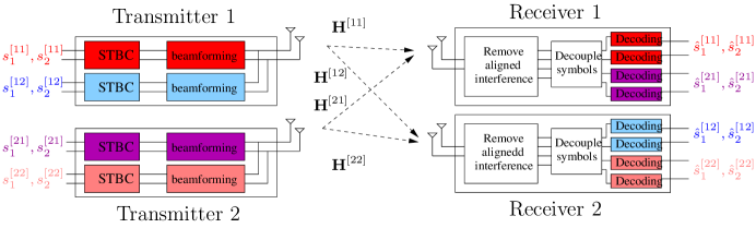
Figure 1: IA designs using Alamouti codes for the $2\times 2$ double-antenna X channel.

The maximum rate of the double-antenna $2\times 2$ X channel is $2\times\frac{4}{3}=\frac{8}{3}$[2]. To achieve this rate, we design each transmitter to send two symbols to each of the two receivers in three channel uses, i.e., $K=2$ and $T=3$. The system diagram is shown in Fig. 1. The transmitted block $\mathbf{X}^{[j]}$ is designed as

$$\mathbf{X}^{[j]}=\sqrt{\frac{3}{4}}\left(\left[\begin{array}[]{cc}s^{[j1]}_{1}&s^{[j1]}_{2}\\ -s^{[j1]*}_{2}&s^{[j1]*}_{1}\\ 0&0\end{array}\right]\mathbf{V}^{[j1]}+\left[\begin{array}[]{cc}0&0\\ -s^{[j2]*}_{2}&s^{[j2]*}_{1}\\ s^{[j2]}_{1}&s^{[j2]}_{2}\end{array}\right]\mathbf{V}^{[j2]}\right),\ j\in\{1,2\},$$ (12)

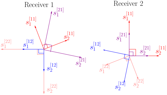
Figure 2: Receiver signal space using the Alamouti designs. Each arrow represent one equivalent channel vector. Each receiver observes a $6$-dimensional signal space. Two dimensions are for aligned interference, and the remained four dimensions are for desired symbols. The equivalent channel vector of $s_{1}^{[ji]}$ is orthogonal to that of $s_{2}^{[ji]}$.

where $\mathbf{V}^{[ji]}\in\mathds{C}^{2\times 2}$ denotes the beamforming matrix from Transmitter $j$ to Receiver $i$. Recall that from (1), the vertical and horizontal dimensions of $\mathbf{X}^{[j]}$ represent temporal and spatial dimensions, respectively. The symbols to Receiver $1$ are encoded by Alamouti designs and transmitted in the first two time slots; whereas the symbols to Receiver $2$ are encoded by Alamouti designs too, but transmitted in the last two time slots. Compared to the designs in (3), our scheme allows each transmitter to send linear combinations of both the original symbols and their conjugate. The beamforming matrices are designed to align $s^{[11]}_{k}$ and $s^{[21]}_{k}$ at Receiver 2, and align $s^{[12]}_{k}$ and $s^{[22]}_{k}$ at Receiver 1 as shown in Fig. 2. Specifically, we design the beamforming matrix as the normalized inversion of the cross channel matrix,

$$\mathbf{V}^{[ji]}=c^{[ji]}\left(\mathbf{H}^{[j\bar{i}]}\right)^{-1},\ j,i\in\{1,2\}$$ (13)

where the index $\bar{i}$ denotes the receiver other than Receiver $i$ and the coefficient $c^{[ji]}=1/\left\|\left(\mathbf{H}^{[j\bar{i}]}\right)^{-1}\right\|$ is to satisfy the power constraint ${\rm tr}\,\left(\mathbf{V}^{[ji]}\mathbf{V}^{[ji]*}\right)=1$. This power constraint implicitly ensures each entry in $\mathbf{V}^{[ji]}$ to be smaller than 1 and avoids high peak powers. The coefficient $\sqrt{\frac{3}{4}}$ in (12) is to normalize the transmit power to $\underset{s_{k}^{[ji]}}{{\mathbb{E}}\,}{\rm tr}\,\left(\mathbf{X}^{[j]}(\mathbf{X}^{[j]})^{*}\right)=3P$ in three channel uses. Inserting (12) into (1), the receive signal blocks can be expanded as

$$\mathbf{Y}^{[1]}=\sum_{j\in\{1,2\}}\sqrt{\frac{3}{4}}\left[\begin{array}[]{cc}s^{[j1]}_{1}&s^{[j1]}_{2}\\ -s^{[j1]*}_{2}&s^{[j1]*}_{1}\\ 0&0\end{array}\right]\tilde{\mathbf{H}}^{[j1]}+\sqrt{\frac{3}{4}}\left[\begin{array}[]{cc}0&0\\ -c^{[11]}s^{[12]*}_{2}-c^{[21]}s^{[22]*}_{2}&c^{[11]}s^{[12]*}_{1}+c^{[21]}s^{[22]*}_{1}\\ c^{[11]}s^{[12]}_{1}+c^{[21]}s^{[22]}_{1}&c^{[11]}s^{[12]}_{2}+c^{[21]}s^{[22]}_{2}\end{array}\right]+\mathbf{W}^{[1]},$$ (20)

$$\mathbf{Y}^{[2]}=\sum_{j\in\{1,2\}}\sqrt{\frac{3}{4}}\left[\begin{array}[]{cc}0&0\\ -s^{[j2]*}_{2}&s^{[j2]*}_{1}\\ s^{[j2]}_{1}&s^{[j2]}_{2}\end{array}\right]\tilde{\mathbf{H}}^{[j2]}+\sqrt{\frac{3}{4}}\left[\begin{array}[]{cc}c^{[12]}s^{[11]}_{1}+c^{[22]}s^{[21]}_{1}&c^{[12]}s^{[11]}_{2}+c^{[22]}s^{[21]}_{2}\\ -c^{[12]}s^{[11]*}_{2}-c^{[22]}s^{[21]*}_{2}&c^{[12]}s^{[11]*}_{1}+c^{[22]}s^{[21]*}_{1}\\ 0&0\end{array}\right]+\mathbf{W}^{[2]},$$ (27)

where $\tilde{\mathbf{H}}^{[ji]}=\mathbf{V}^{[ji]}\mathbf{H}^{[ji]}$ denotes the equivalent channels that incorporate beamforming matrices. In the above equations, the first term represents desired symbols, whereas the second term represents interference. It can be observed that the interference term still has Alamouti structure, since $c^{[ji]}$ is a real number. In other words, $s^{[12]}_{k}$ and $s^{[22]}_{k}$ are aligned at Receiver 1, while $s^{[11]}_{k}$ and $s^{[21]}_{k}$ are aligned at Receiver 2. We can further convert the system equations into vector forms to study the receive signal space. Let us denote the $t$th row of $\mathbf{Y}^{[i]}$ and $\mathbf{W}^{[i]}$ be $\mathbf{y}_{t}^{[i]}$ and $\mathbf{w}_{t}^{[i]}$, respectively, where $t\in\{1,2,3\}$. Denote the aligned interfering symbols as $I_{k}^{[1]}=c^{[11]}s^{[12]}_{k}+c^{[21]}s^{[22]}_{k},I_{k}^{[2]}=c^{[12]}s^{[11]}_{k}+c^{[22]}s^{[21]}_{k}$, and the $(m,n)$th entry of $\tilde{\mathbf{H}}^{[ji]}$ as $\tilde{{h}}^{[ji]}_{mn}$. The receiver calculates $\tilde{\mathbf{y}}^{[i]}=\mathrm{vec}\left(\left[\mathbf{y}_{1}^{[i]*},(-1)^{i}\left(\mathbf{y}_{2}^{[i]}\right)^{\mathrm{T}},\mathbf{y}_{3}^{[i]*}\right]^{*}\right)$, and Eqns. (20) and (27) can be converted as

$$\tilde{\mathbf{y}}^{[1]}=\sqrt{\frac{3}{4}}\left[\begin{array}[]{cccccc}\tilde{h}^{[11]}_{11}&\tilde{h}^{[11]}_{21}&\tilde{h}^{[21]}_{11}&\tilde{h}^{[21]}_{21}&0&0\\ -\tilde{h}^{[11]*}_{21}&\tilde{h}^{[11]*}_{11}&-\tilde{h}^{[21]*}_{21}&\tilde{h}^{[21]*}_{11}&0&1\\ 0&0&0&0&1&0\\ \tilde{h}^{[11]}_{12}&\tilde{h}^{[11]}_{22}&\tilde{h}^{[21]}_{12}&\tilde{h}^{[21]}_{22}&0&0\\ -\tilde{h}^{[11]*}_{22}&\tilde{h}^{[11]*}_{12}&-\tilde{h}^{[21]*}_{22}&\tilde{h}^{[21]*}_{12}&-1&0\\ 0&0&0&0&0&1\end{array}\right]\left[\begin{array}[]{c}s^{[11]}_{1}\\ s^{[11]}_{2}\\ s^{[21]}_{1}\\ s^{[21]}_{2}\\ I^{[1]}_{1}\\ I_{2}^{[1]}\end{array}\right]+\tilde{\mathbf{w}}^{[1]}$$ (40)

at Receiver $1$, and

$$\tilde{\mathbf{y}}^{[2]}=\sqrt{\frac{3}{4}}\left[\begin{array}[]{cccccc}0&0&0&0&1&0\\ \tilde{h}^{[12]*}_{21}&-\tilde{h}^{[12]*}_{11}&\tilde{h}^{[22]*}_{21}&-\tilde{h}^{[22]*}_{11}&0&-1\\ \tilde{h}^{[12]}_{11}&\tilde{h}^{[12]}_{21}&\tilde{h}^{[22]}_{11}&\tilde{h}^{[22]}_{21}&0&0\\ 0&0&0&0&0&1\\ \tilde{h}^{[12]*}_{22}&-\tilde{h}^{[12]*}_{12}&\tilde{h}^{[22]*}_{22}&-\tilde{h}^{[22]*}_{12}&1&0\\ \tilde{h}^{[12]}_{12}&\tilde{h}^{[12]}_{22}&\tilde{h}^{[22]}_{12}&\tilde{h}^{[22]}_{22}&0&0\end{array}\right]\left[\begin{array}[]{c}s^{[12]}_{2}\\ s^{[12]}_{1}\\ s^{[22]}_{1}\\ s^{[22]}_{2}\\ I_{1}^{[2]}\\ I_{2}^{[2]}\end{array}\right]+\tilde{\mathbf{w}}^{[2]}$$ (53)

at Receiver $2$, where $\tilde{\mathbf{y}}^{[i]},\tilde{\mathbf{w}}^{[i]}\in\mathds{C}^{6\times 1}$ and $\tilde{\mathbf{w}}^{[i]}=\mathrm{vec}\left(\left[\mathbf{w}_{1}^{[i]*},(-1)^{i}\mathbf{w}_{2}^{[i]\mathrm{T}},\mathbf{w}_{3}^{[i]*}\right]^{*}\right)$ denotes the equivalent AWGN vector at Receiver $i$. It can be observed that the equivalent channel vectors of $s_{1}^{[ji]}$ and $s_{2}^{[ji]}$ (correspond to the $(2j-1)$ and $(2j)$th columns in the equivalent channel matrix) are orthogonal. Thus, the desired links are enhanced by embedding Alamouti codes into alignment. The receive signal space is illustrated in Fig. 2.

In what follows, we explain receiver decoding using IC originally proposed for MAC[9]. Although IC is essentially ZF, IC avoids high dimensional matrix processing (simplify the computation of matrix inversion in the projection matrix). Since the designs of the network is symmetric to each receiver, we focus only on the processing at Receiver 1 to simplify presentation. Processing at Receiver 2 is similar and has the same performance as that of Receiver 1. Since we only discuss Receiver 1, in what follows, we will remove receiver index $i$ from $\tilde{\mathbf{y}}^{[i]}$ and $\tilde{\mathbf{w}}^{[i]}$ to simplify the presentation. The IC has the following two steps:

III-A1 Step 1: Remove aligned interference

Let the $\tau$th entry of $\tilde{\mathbf{y}}$ and $\tilde{\mathbf{w}}$ in (40) be $\tilde{y}_{\tau}$ and $\tilde{w}_{\tau}$, respectively. Since the equivalent channels for interference $I_{1}^{[1]}$ and $I_{2}^{[1]}$ are constant in (40), the aligned interference $I_{1}^{[1]}$ and $I_{2}^{[1]}$ can be cancelled by

$$\left[\begin{array}[]{cccc}\tilde{y}_{1}&\tilde{y}_{2}+\tilde{y}_{6}&\tilde{y}_{4}&\tilde{y}_{5}-\tilde{y}_{3}\end{array}\right]^{\mathrm{T}}.$$ (55)

Let $\hat{\mathbf{y}}_{1}=\left[\begin{array}[]{cc}\tilde{y}_{1}&\tilde{y}_{2}+\tilde{y}_{6}\end{array}\right]^{\mathrm{T}},\hat{\mathbf{y}}_{2}=\left[\begin{array}[]{cc}\tilde{y}_{4}&\tilde{y}_{5}-\tilde{y}_{3}\end{array}\right]^{\mathrm{T}},\hat{\mathbf{w}}_{1}=\left[\begin{array}[]{cc}\tilde{w}_{1}&\tilde{w}_{2}+\tilde{w}_{6}\end{array}\right]^{\mathrm{T}},\ \hat{\mathbf{w}}_{2}=\left[\begin{array}[]{cc}\tilde{w}_{4}&\tilde{w}_{5}-\tilde{w}_{3}\end{array}\right]^{\mathrm{T}}$. The resulting equivalent system equation can be simplified as

$$\left[\begin{array}[]{c}\hat{\mathbf{y}}_{1}\\ \hat{\mathbf{y}}_{2}\end{array}\right]=\sqrt{\frac{3}{4}}\left(\left[\begin{array}[]{c}\hat{\mathbf{H}}^{[11]}_{1}\\ \hat{\mathbf{H}}^{[11]}_{2}\end{array}\right]\left[\begin{array}[]{c}s^{[11]}_{1}\\ s^{[11]}_{2}\end{array}\right]+\left[\begin{array}[]{c}\hat{\mathbf{H}}^{[21]}_{1}\\ \hat{\mathbf{H}}^{[21]}_{2}\end{array}\right]\left[\begin{array}[]{c}s^{[21]}_{1}\\ s^{[21]}_{2}\end{array}\right]\right)+\left[\begin{array}[]{c}\hat{\mathbf{w}}_{1}\\ \hat{\mathbf{w}}_{2}\end{array}\right],$$ (68)

where $\hat{\mathbf{H}}^{[j1]}_{n}\in\mathds{C}^{2\times 2}$ has an Alamouti structure

$$\hat{\mathbf{H}}^{[j1]}_{n}=\left[\begin{array}[]{cc}\tilde{h}_{1n}^{[j1]}&\tilde{h}^{[j1]}_{2n}\\ \tilde{h}_{2n}^{[j1]*}&-\tilde{h}_{1n}^{[j1]*}\end{array}\right],\ j\in\{1,2\}.$$ (71)

III-A2 Step 2: Decouple symbols from different transmitters

The system equation in (68) is similar to that of a MAC system with two double-antenna transmitters and one double-antenna receiver. The equivalent noise vector $\left[\hat{\mathbf{w}}_{1}^{\mathrm{T}}\ \hat{\mathbf{w}}_{2}^{\mathrm{T}}\right]^{\mathrm{T}}$ is white but does not have identical variances for each entry. IC is applicable to decouple $s^{[11]}_{1}$ and $s^{[11]}_{2}$ from $s^{[21]}_{1}$ and $s^{[21]}_{2}$. Receiver 1 conducts

$$\underset{\hat{\mathbf{y}}}{\underbrace{\frac{\hat{\mathbf{H}}_{1}^{[21]*}}{\left\|\hat{\mathbf{H}}_{1}^{[21]}\right\|^{2}}\hat{\mathbf{y}}_{1}-\frac{\hat{\mathbf{H}}_{2}^{[21]*}}{\left\|\hat{\mathbf{H}}_{2}^{[21]}\right\|^{2}}\hat{\mathbf{y}}_{2}}}= \sqrt{\frac{3}{4}}\underset{\hat{\mathbf{H}}}{\underbrace{\left(\frac{\hat{\mathbf{H}}_{1}^{[21]*}\hat{\mathbf{H}}_{1}^{[11]}}{\left\|\hat{\mathbf{H}}_{1}^{[21]}\right\|^{2}}-\frac{\hat{\mathbf{H}}_{2}^{[21]*}\hat{\mathbf{H}}_{2}^{[11]}}{\left\|\hat{\mathbf{H}}_{2}^{[21]}\right\|^{2}}\right)}}\left[\begin{array}[]{c}s^{[11]}_{1}\\ s^{[11]}_{2}\end{array}\right]+\frac{\hat{\mathbf{H}}_{1}^{[21]*}\hat{\mathbf{w}}_{1}}{\left\|\hat{\mathbf{H}}_{1}^{[21]}\right\|^{2}}-\frac{\hat{\mathbf{H}}_{2}^{[21]*}\hat{\mathbf{w}}_{2}}{\left\|\hat{\mathbf{H}}_{2}^{[21]}\right\|^{2}}.$$ (74)

Due to the completeness of matrix addition, matrix multiplication, and scalar multiplication of the Alamouti matrix, the equivalent channel matrix $\hat{\mathbf{H}}$ still has the Alamouti structure. Thus, $s^{[11]}_{k}$ can be decoded by

$$s^{[11]}_{k}=\arg\max_{s}\hat{\mathbf{h}}_{k}^{*}\hat{\mathbf{y}}s,k\in\{1,2\},$$ (75)

where $\hat{\mathbf{h}}_{k}$ denotes the $k$th column of $\hat{\mathbf{H}}$. Note that the decoding complexity is symbol-by-symbol. Similar to (74), we can decouple $s^{[21]}_{1}$ and $s^{[21]}_{2}$ by calculating $\frac{\hat{\mathbf{H}}_{1}^{[11]*}}{\left\|\hat{\mathbf{H}}_{1}^{[11]}\right\|^{2}}\hat{\mathbf{y}}_{1}-\frac{\hat{\mathbf{H}}_{2}^{[11]*}}{\left\|\hat{\mathbf{H}}_{2}^{[11]}\right\|^{2}}\hat{\mathbf{y}}_{2}$. Similar operations can be performed at Receiver 2 to decode $s^{[12]}_{k}$ and $s^{[22]}_{k}$. Therefore, four procedures of symbol-by-symbol decoding are required at each receiver to recover desired symbols.

III-B Performance analysis

This subsection provides diversity gain analysis in the short-term regime. Further, we show that the proposed scheme does not lose the DoF gain in the long-term regime.

In a point-to-point channel, diversity gain is defined as the asymptotical slope of BER with respect to the receive SNR in the high SNR regime. For our considered network model, we define diversity gain as the asymptotical rate of BER with respect to power $P$ for the symbol-by-symbol decoding given in (75). A diversity calculation technique using instantaneous normalized receive SNR was proposed in [22] for short-term communication systems. For a vector channel with an equivalent system equation $\mathbf{y}=\mathbf{h}s+\mathbf{w}$, where $\mathbf{y},\mathbf{h},s,\mathbf{w}$ denote the receive signal vector, the equivalent channel vector, transmit symbol, and the equivalent noise vector, respectively. The instantaneous normalized receive SNR for symbol $s$ is defined as $\gamma=\mathbf{h}^{*}\mathbf{\Sigma}^{-1}\mathbf{h}$, where $\mathbf{\Sigma}$ is the covariance matrix of $\mathbf{w}$. Diversity gain for the maximum-likelihood (ML) decoding of this equivalent system equation can be calculated as

$$d=-\lim_{\epsilon\rightarrow 0}\frac{\log P(\gamma<\epsilon)}{\log\epsilon},$$ (76)

where $P(\gamma<\epsilon)$ denotes the outage probability of $\gamma$. Using this technique, we present the following theorems.

Theorem 1

In the short-term regime, the JaSh scheme achieves a diversity gain no more than $1$ for the $2\times 2$ double-antenna X channel.

Proof:

See Appendix B for proof. ∎

The intuition of the theorem can be explained as follows. The receiver observes a six-dimensional signal space, in which two dimensions are for aligned interference and four dimensions are for desired symbols. The equivalent channel vectors for desired symbols are randomly distributed in the receive signal space as shown from (305) (the beamforming vectors $\mathbf{u}_{1},\mathbf{u}_{2}$ depend on channels of $\mathbf{H}^{[21]},\mathbf{H}^{[12]},\mathbf{H}^{[22]}$, while the equivalent channel matrix is $\mathbf{H}^{[11]}$ for all desired symbols). By a ZF receiver, the projection to cancel the aligned interference and decouple the desired symbols incurs SNR loss. Thus, the resulting diversity gain is 1.

Theorem 2

In the short-term regime, the proposed alignment method with Alamouti designs achieves a diversity gain of 2 for the $2\times 2$ double-antenna X channel.

Proof:

See Appendix D for proof. ∎

This diversity improvement can be intuitively explained as follows. Compared to the JaSh scheme, two desired symbols are orthogonal (See (40) and (53)) due to the use of Alamouti structure at transmitters. After removing aligned interference, the system equation in (68) is similar to a MAC with two double-antenna transmitters and one double-antenna receiver. The IC uses one receive antenna to decouple symbols. Then, the receive diversity of the proposed scheme is 1. A transmit diversity gain of 2 is achievable through Alamouti designs. The total diversity gain is the product of the transmit diversity and receiver diversity, i.e., it is 2.

Next, we discuss the proposed scheme in the long-term regime. In this case, Gaussian codebooks can be used for $s_{k}^{[ji]}$, and transmitters adjust the rate over infinite sets of Gaussian codebooks based on CSIT and the transmit power. The network can reliably transmit information without outage assuming infinite coding. The DoF gain is defined as the asymptotical ratio between the bit-rate and $\log P$[12]. For our proposed scheme, each symbol $s_{k}^{[ji]}$ can be viewed as a data stream whose bit-rate can be adjusted adaptively. The achievable DoF gain is shown in the following theorem.

Theorem 3

In the long-term regime, the proposed alignment method with Alamouti designs achieves the maximum DoF gain of $\frac{8}{3}$ for the $2\times 2$ double-antenna X channel.

Proof:

Since interferring symbols are aligned by the design and appear in different temporal dimensions compared to the desired symbol (At Receiver 1, the desired symbols are received in time Slots 1 and 2, and interferring symbols are received in time Slots 2 and 3), the desired symbols can be decoupled from the interferring symbols. Then, it is sufficient to show the linear independence among the desired symbols. We only show the linear independence at Receiver 1, since the channel matrix of the four desired symbols has the same structure at Receiver 2. We need to prove that the following $4\times 4$ matrix has full rank

$$\left[\begin{array}[]{cccc}\tilde{h}^{[11]}_{11}&\tilde{h}^{[11]}_{21}&\tilde{h}^{[21]}_{11}&\tilde{h}^{[21]}_{21}\\ -\tilde{h}^{[11]*}_{21}&\tilde{h}^{[11]*}_{11}&-\tilde{h}^{[21]*}_{21}&\tilde{h}^{[21]*}_{11}\\ \tilde{h}^{[11]}_{12}&\tilde{h}^{[11]}_{22}&\tilde{h}^{[21]}_{12}&\tilde{h}^{[21]}_{22}\\ -\tilde{h}^{[11]*}_{22}&\tilde{h}^{[11]*}_{12}&-\tilde{h}^{[21]*}_{22}&\tilde{h}^{[21]*}_{12}\end{array}\right].$$ (81)

This is straightforward since the determinant of the above matrix is a polynomial function of eight entries $\tilde{h}^{[j1]}_{mn}$ with $j,m,n\in\{1,2\}$. Recall that $\tilde{h}^{[11]}_{mn}$ depends on channel matrices $\mathbf{H}^{[11]}$ and $\mathbf{H}^{[12]}$, while $\tilde{h}^{[21]}_{mn}$ depends on $\mathbf{H}^{[21]}$ and $\mathbf{H}^{[22]}$, with all channel matrices being independently drawn. The equivalent channels $\tilde{h}^{[11]}_{mn}$ are independent from $\tilde{h}^{[21]}_{mn}$. Then, the determinant polynomial is either 0 or non-zero for all values of $\tilde{h}^{[j1]}_{mn}$ with probability 1[23]. When $\tilde{h}^{[11]}_{11}=\tilde{h}^{[21]}_{12}=1$ and $\tilde{h}^{[11]}_{21}=\tilde{h}^{[11]}_{12}=\tilde{h}^{[11]}_{22}=\tilde{h}^{[21]}_{11}=\tilde{h}^{[21]}_{21}=\tilde{h}^{[21]}_{22}=0$, the matrix in (81) becomes an identity matrix and full rank. Thus, the determinant is not a zero polynomial and the matrix in (81) is full rank with probability 1.

For each data stream $s_{k}^{[ji]}$, a rate that grows linearly with $\log P$ can be reliably supported. Since $8$ streams are sent over the network in $3$ channel uses, the proposed scheme achieves the DoF gain of $\frac{8}{3}$. The outerbound on the DoF gain of the $2\times 2$ double-antenna X channel was characterized in [2] to be $\frac{8}{3}$. Therefore, the proposed scheme achieves the maximum DoF gain. ∎

IV Alamouti-coded Transmission for Cellular Networks

In this section, we discuss two types of cellular networks: the IMAC and IBC networks[15], where interference from a neighboring cell degrades in-cell communication. Again, the use of Alamouti codes together with IA can bring the maximum transmission rate and a diversity gain of $2$. We explain the network models and show the maximum DoF gain in Subsection IV-A. Since the X channel is a special case of the IMAC, we briefly describe its transmission in Subsection IV-B. Transmission in the IBC is more challenging compared to the IMAC because of the required designs of imperfect alignment. Description for alignment in IBC is contained in Subsection IV-C. Regarding channel information, each MS requires only the knowledge of the interferring link connected to itself, and each base station (BS) needs channel information within its cell as well as the knowledge of its MSs’ beamformers.

IV-A The IMAC and IBC network models

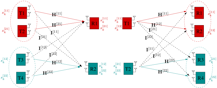
Figure 3: Network models of the two-cell IMAC and the IBC. In each cell, one BS is serving two users. Transmission in one cell creates interference to the other cell. The desired links are represented by solid lines, whereas interferring links are represented by dashed lines.

Consider a two-cell IMAC as illustrated in the left side of Fig. 3. In each cell, one BS serves two MSs. All nodes are equipped with two antennas. In the IMAC, we can use the receiver’s index for the cell index, since there is only one receiver in each cell. In Cell $i$, transmitter $j$ has independent symbols $s_{k}^{[ji]}$ to send to Receiver $i$, where $i,j\in\{1,2\}$. The desired links are described by channel matrix $\mathbf{H}^{[ji]}$, where $\mathbf{H}^{[ji]}\in\mathds{C}^{2\times 2}$. Due to the simultaneous transmission, Cell 1 creates co-channel interference to Cell 2, and similarly does Cell 2 to Cell 1. The interferring link from Transmitter $j$ to Cell $i$ is described by channel matrix $\mathbf{I}^{[ji]}$, where $\mathbf{I}^{[ji]}\in\mathds{C}^{2\times 2}$. We assume that all entries in channel matrices have i. i. d. $\mathcal{CN}(0,1)$ distribution, and remain constant during the transmission. The reciprocal channel of the IMAC is an IBC, where the directions of communication are reversed. Contrary to the IMAC, in the IBC, we can use the transmitter’s index for the cell index, since there is only one transmitter in each cell. Transmitter $j$ sends independent symbols $s_{k}^{[ji]}$ to Receiver $i$ in Cell $j$ through link $\mathbf{H}^{[ji]}$, and simultaneously interferes User $i$ in the other Cell $\bar{j}$ through link $\mathbf{I}^{[\bar{j}i]}$. We can use similar notations as that of the IMAC for the IBC with an exchange of the cell and user indices. The IBC and adopted notations are shown in the right side of Fig. 3.

IA is considered for the IMAC in [15] and the IBC in [18, 24]. These two channel models are introduced for frequency selective channels in [15], where the duality between these two channels is also demonstrated. Transmission in a two-cell IBC is studied in [24] with the number of BS antennas larger than the number of receive antennas. Our paper considers a MIMO setting where all nodes have equal number of antennas. First, we show the outerbound on the DoF gains. In the proof, we assume that $s_{k}^{[ji]}$ operates in the long-term region and carries one DoF gain.

Theorem 4

For a two-cell IBC with two users in each cell and two antennas at each node, let $d^{[ji]}$ be the DoF gain sent from Transmitter $j$ to Receiver $i$ in Cell $j$. The DoF gain region $\mathcal{D}^{\mathrm{IBC}}$ is

$$d^{[11]}+d^{[21]}+d^{[22]}\leq 2,$$ (82)

$$d^{[12]}+d^{[21]}+d^{[22]}\leq 2,$$ (83)

$$d^{[21]}+d^{[11]}+d^{[12]}\leq 2,$$ (84)

$$d^{[22]}+d^{[11]}+d^{[12]}\leq 2.$$ (85)

Proof:

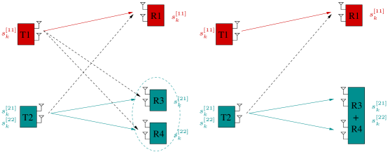
Figure 4: Proof of the outerbound on the DoF region of the IBC: a modified IBC (left side) and a Z channel (right side).

The proof is similar to that of the outerbound on X channels[2]. Since the network is symmetric for each cell and each receiver, we only show inequality (82) and the other three inequalities hold by similar arguments. We argue that the DoF gain region $\underset{\mathcal{D}^{\mathrm{IBC}}}{\max}\left(d^{[11]}+d^{[21]}+d^{[22]}\right)$ can be outerbounded by those of two channels illustrated in Fig. 4. The first outerbound is a modified IBC without Receiver 2 in Cell 1. BS1 sends messages only to Receiver 1. Obviously, any reliable coding schemes in the IBC can be used reliably in the modified IBC. Then, let $\mathcal{D}^{\mathrm{IBC}^{\prime}}$ denote the DoF gain regions of the modified IBC, we have $\underset{\mathcal{D}^{\mathrm{IBC}}}{\max}\left(d^{[11]}+d^{[21]}+d^{[22]}\right)\leq\underset{\mathcal{D}^{\mathrm{IBC}^{\prime}}}{\max}\left(d^{[11]}+d^{[21]}+d^{[22]}\right)$. We can further outerbound the DoF region of the modified IBC using the Z channel by allowing receivers in Cell 2 to cooperate (right side of Fig. 4). This is because any reliable coding schemes for the modified IBC can be used in the Z channel by adding interference at receivers in Cell 2 and decoding as if R3 and R4 are distributed. Let the DoF gain region of the Z channel be $\mathcal{D}^{\mathrm{Z}}$. From Corollary 1 in [2], we have $\underset{\mathcal{D}^{\mathrm{Z}}}{\max}\left(d^{[11]}+d^{[21]}+d^{[22]}\right)\leq 2$, since both BS2 and R1 have two antennas. It follows $\underset{\mathcal{D}^{\mathrm{IBC}}}{\max}\left(d^{[11]}+d^{[21]}+d^{[22]}\right)\leq\underset{\mathcal{D}^{\mathrm{Z}}}{\max}\left(d^{[11]}+d^{[21]}+d^{[22]}\right)\leq 2$. ∎

Due to the duality between the IMAC and the IBC, the same DoF gain region holds for the IMAC. Combing (82), (83), (84), (85) results in $d^{[11]}+d^{[12]}+d^{[21]}+d^{[22]}\leq\frac{8}{3}$.

IV-B Transmission methods in the IMAC

The maximum rate for the considered IMAC is $\frac{8}{3}$ symbols per channel use. Noticing that the double-antenna $2\times 2$ X channel is a special scenario of the two-cell IMAC when $\mathbf{I}^{[ji]}=\mathbf{H}^{[j\bar{i}]}$. Then, it is straightforward to use the method we have proposed for the X channel for the two-cell IMAC. Specifically, two symbols $k\in\{1,2\}$, encoded in Alamouti codes, are transmitted in three channel uses. Transmission in Cell $1$ occurs in the first two time slots, while transmission in Cell $2$ occurs in the last two time slots. For Transmitter $j$ in Cell $i$, the normalized inversion of $\mathbf{I}^{[ji]}$ is used as the alignment precoder. Then, four interferring symbols are aligned into two dimensions. Since the X channel is a special case of the considered IMAC, a diversity gain of 2 is achievable at the maximum rate of $\frac{8}{3}$ symbols per channel use. Diversity analysis for the IMAC using the proposed method is similar to Theorem 3.

IV-C Transmission methods in the IBC

In what follows, we discuss the extension to the two-cell IBC. By duality of reciprocal channels, the maximum rate of the two-cell IBC is also $\frac{8}{3}$ symbols per channel use. Let the transmission duration $T$ be three channel uses. To achieve the maximum rate, each transmitter sends two symbols to each receiver. In total, $8$ symbols are transmitted over the network in three channel uses, which amounts to the rate of $\frac{8}{3}$ symbols per channel use. Since each receiver is equipped with two antennas and receives in three time slots, a six-dimensional signal space is created. Each receiver intends to decode two symbols and leaves the remaining four-dimensional subspace for six interfering symbols (two symbols are for the other receiver in the same cell, i.e., intra-cell interference, and four symbols are from the other cell, i.e., inter-cell interference). Thus, we need an alignment design that aligns six symbols in four-dimensional subspace. Such an imperfect alignment design cannot be trivially extended from the proposed method for X channels, where interference is completely aligned.

We use the method constructing a dual system from the original system as proposed in [11]. The methodology has been used to design the dual Alamouti codes and the downlink IC method, where receiver processing is totally blind of channel information. The constructed scheme can bring to the dual system the same diversity gain as in the original system. We use the transmission method in the IMAC as the original system to derive its dual system. The derivation is involved, and we directly present the transmission method in the two-cell IBC. Note that a diversity gain of 2 is achievable for the dual system, following the definition of dual systems with ZF designs (Definition 1 and Proposition 1 in [11]).

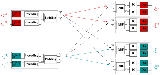
Figure 5: System diagram of the proposed transmission method in the two-cell IBC.

The system diagram is shown in Fig. 5. Let the transmit block be $\mathbf{X}^{[j]}$, where $\mathbf{X}^{[j]}\in\mathds{C}^{3\times 2}$. The receive block at Receiver $i$ in Cell $j$ can be written as

$$\mathbf{Y}^{[ji]}=\mathbf{X}^{[j]}\mathbf{H}^{[ji]}+\mathbf{X}^{[\bar{j}]}\mathbf{I}^{[ji]}+\mathbf{W}^{[ji]},$$ (86)

where $\mathbf{W}^{[ji]}\in\mathds{C}^{3\times 2}$ denotes the AWGN matrix. Different from the IMAC, we use the inversion of the interferring link as the receive beamforming matrix

$$\underset{\tilde{\mathbf{Y}}^{[ji]}}{\underbrace{\mathbf{Y}^{[ji]}\left(\mathbf{I}^{[ji]}\right)^{-1}}}=\mathbf{X}^{[j]}\underset{\tilde{\mathbf{H}}^{[ji]}}{\underbrace{\mathbf{H}^{[ji]}\left(\mathbf{I}^{[ji]}\right)^{-1}}}+\mathbf{X}^{[\bar{j}]}+\underset{\tilde{\mathbf{W}}^{[ji]}}{\underbrace{\mathbf{W}^{[ji]}\left(\mathbf{I}^{[ji]}\right)^{-1}}}.$$ (87)

By such receive beamforming matrices, the equivalent interferring links are identical at both receivers in one cell. This helps the design of alignment precoder, as will be explained later. The transmitter design is based on the equivalent channel matrix $\tilde{\mathbf{H}}^{[ji]}\in\mathds{C}^{2\times 2}$. Each transmitter collects two symbols $s_{k}^{[ji]}$ ($k\in\{1,2\}$), modulated by PSK constellations, for each receiver in the cell. The symbols are encoded using Alamouti codes followed by linear precoding as

$$\left[\begin{array}[]{cc}x_{11}^{[j]}&x_{12}^{[j]}\\ x_{21}^{[j]}&x_{22}^{[j]}\end{array}\right]=\underset{\mathbf{S}^{[j1]}}{\underbrace{\left[\begin{array}[]{cc}s_{1}^{[j1]}&s_{2}^{[j1]}\\ -s_{2}^{[j1]*}&s_{1}^{[j1]*}\end{array}\right]}}\mathbf{P}^{[j1]}+\underset{\mathbf{S}^{[j2]}}{\underbrace{\left[\begin{array}[]{cc}s_{1}^{[j2]}&s_{2}^{[j2]}\\ -s_{2}^{[j2]*}&s_{1}^{[j2]*}\end{array}\right]}}\mathbf{P}^{[j2]},$$ (94)

where $\mathbf{P}^{[ji]}\in\mathds{C}^{2\times 2}$ are the precoding matrix for Receiver $i$ in Cell $j$. We use the precoding matrices from the downlink IC method[11]. Let the $(m,n)$the entry of $\tilde{\mathbf{H}}^{[ji]}$ be $\tilde{h}^{[ji]}_{mn}$. The matrix $\mathbf{P}^{[ji]}$ is designed as

$$\mathbf{P}^{[ji]}=\alpha^{[ji]}\left(\frac{\hat{\mathbf{H}}^{[ji]*}_{1}\hat{\mathbf{H}}^{[j\bar{i}]}_{1}}{\left\|\tilde{\mathbf{h}}^{[j\bar{i}]}_{1}\right\|^{2}}-\frac{\hat{\mathbf{H}}^{[ji]*}_{2}\hat{\mathbf{H}}^{[j\bar{i}]}_{2}}{\left\|\tilde{\mathbf{h}}^{[j\bar{i}]}_{2}\right\|^{2}}\right)\left[\begin{array}[]{cc}\frac{\tilde{h}^{[j\bar{i}]*}_{11}}{\left\|\tilde{\mathbf{h}}^{[j\bar{i}]}_{1}\right\|^{2}}&-\frac{\tilde{h}^{[j\bar{i}]*}_{21}}{\left\|\tilde{\mathbf{h}}^{[j\bar{i}]}_{2}\right\|^{2}}\\ \frac{\tilde{h}^{[j\bar{i}]*}_{12}}{\left\|\tilde{\mathbf{h}}^{[j\bar{i}]}_{1}\right\|^{2}}&-\frac{\tilde{h}^{[j\bar{i}]*}_{22}}{\left\|\tilde{\mathbf{h}}^{[j\bar{i}]}_{2}\right\|^{2}}\end{array}\right],$$ (97)

where $\alpha^{[ji]}\in\mathds{R}$ denotes a power control parameter for Receiver $i$ in Cell $j$, $\tilde{\mathbf{h}}^{[ji]}_{m}$ denotes the $m$th row in $\tilde{\mathbf{H}}^{[ji]}$, and

$$\hat{\mathbf{H}}_{m}^{[ji]}=\left[\begin{array}[]{cc}\tilde{h}^{[ji]}_{m1}&\tilde{h}^{[ji]}_{m2}\\ -\tilde{h}^{[ji]*}_{m2}&\tilde{h}^{[ji]*}_{m1}\end{array}\right],\ m\in\{1,2\}.$$ (100)

For the details behind the derivation of the designs in (97), the interested reader is referred to [11]. Here, we only explain how alignment is created. The symbols $x_{tm}^{[ji]}$ in (94) are rearranged to generate the transmit block $\mathbf{X}^{[j]}$,

$$\mathbf{X}^{[1]}=\left[\begin{array}[]{cc}x^{[1]}_{11}&x^{[1]}_{12}\\ x^{[1]}_{21}&x^{[1]}_{22}\\ x^{[1]*}_{22}&-x^{[1]*}_{21}\end{array}\right],\ \mathbf{X}^{[2]}=\left[\begin{array}[]{cc}-x^{[2]*}_{22}&x^{[2]*}_{21}\\ x^{[2]}_{21}&x^{[2]}_{22}\\ x^{[2]}_{11}&x^{[2]}_{12}\end{array}\right].$$ (107)

The four entries in the left-side of (94) carry four independent symbols. Recall that the vertical dimension of $\mathbf{X}^{[j]}$ refers to the temporal dimension. From (107), Transmitter $1$ sends four symbols in the first two time slots. In time Slot $3$, redundant symbols are transmitted to make the submatrix in time Slots $2$ and $3$ have the swapped Alamouti structure, i.e.,

$$\left[\begin{array}[]{cc}a&b\\ b^{*}&-a^{*}\end{array}\right],$$ (110)

which can be obtained by swapping the columns of an Alamouti matrix. Transmitter $2$ sends four symbols in the last two time slots. In time Slot $1$, redundant symbols are transmitted to make the submatrix in time Slots $1$ and $2$ also have the swapped Alamouti structure. It will be shown that the swapped Alamouti structure aligns the interference as well.

Let us further discuss receiver operations. Let the $(t,n)$th entry of $\tilde{\mathbf{Y}}^{[ji]}$ in (87) be $\tilde{y}^{[ji]}_{tn}$. The receivers in Cell $1$ extract useful symbols using signals received in the first two time slots as

$$\left[\begin{array}[]{cc}\hat{y}^{[1i]}_{1}&\hat{y}^{[1i]}_{2}\end{array}\right]=\left[\begin{array}[]{cc}\tilde{y}^{[1i]}_{11}+\tilde{y}^{[1i]*}_{22}&\tilde{y}^{[1i]}_{12}-\tilde{y}^{[1i]*}_{21}\end{array}\right],\ i\in\{1,2\}.$$ (113)

In Cell $2$, receivers calculate $\left[\begin{array}[]{cc}\hat{y}^{[2i]}_{1}&\hat{y}^{[2i]}_{2}\end{array}\right]=\left[\begin{array}[]{cc}\tilde{y}^{[2i]}_{31}+\tilde{y}^{[2i]*}_{22}&\tilde{y}^{[2i]}_{32}-\tilde{y}^{[2i]*}_{21}\end{array}\right],\ i\in\{1,2\}$ using signals received in the last two time slots. Decoding of symbol $s_{k}^{[ji]}$ is performed by $\underset{s}{\max}\hat{y}^{[ji]}_{k}s^{*}.$ The simple receiver operations are due to the precoder designs in (94). From the receiver operations in (87), (113), and the decoding, only the knowledge of $\mathbf{I}^{[ji]}$ is required at Receiver $i$ in Cell $j$. Transmitter operations are based on $\tilde{\mathbf{H}}^{[ji]}$. Then, the knowledge of $\mathbf{H}^{[ji]}$ and $\mathbf{I}^{[ji]}$ for $i\in\{1,2\}$ is required at Transmitter $j$.

IV-C1 Alignment pattern

In what follows, we explain how the proposed method aligns six symbols in a four-dimensional subspace and how Alamouti designs are used to protect desired symbols. First, we introduce some intermediate variables to simplify notations. Note that from (100) and (94), both the matrices $\hat{\mathbf{H}}_{m}^{[ji]}$ and $\mathbf{S}^{[ji]}$ have the Alamouti structure. Since matrix multiplication and addition are closed for two Alamouti matrices, we can define $c_{k}^{[ji]}\in\mathds{C}$

$$\left[\begin{array}[]{cc}c_{1}^{[ji]}&c_{2}^{[ji]}\\ -c_{2}^{[ji]*}&c_{1}^{[ji]*}\end{array}\right]=\alpha^{[ji]}\mathbf{S}^{[ji]}\left(\frac{\hat{\mathbf{H}}^{[ji]*}_{1}\hat{\mathbf{H}}^{[j\bar{i}]}_{1}}{\left\|\tilde{\mathbf{h}}^{[j\bar{i}]}_{1}\right\|^{2}}-\frac{\hat{\mathbf{H}}^{[ji]*}_{2}\hat{\mathbf{H}}^{[j\bar{i}]}_{2}}{\left\|\tilde{\mathbf{h}}^{[j\bar{i}]}_{2}\right\|^{2}}\right)$$ (116)

as the rotated symbols of $s_{k}^{[ji]}$. Without loss of generality, we only show alignment at receivers in Cell $1$. Using $c_{k}^{[ji]}$, we can expand the receive signals of Receiver 1 in (87) using $c_{k}^{[ji]}$ as

$$\left[\begin{array}[]{cc}\tilde{y}_{11}^{[11]}&\tilde{y}_{12}^{[11]}\\ \tilde{y}_{21}^{[11]}&\tilde{y}_{22}^{[11]}\end{array}\right]=\left(\sum_{i=1,2}\left[\begin{array}[]{cc}c^{[1i]}_{1}&c^{[1i]}_{2}\\ -c^{[1i]*}_{2}&c^{[1i]*}_{1}\end{array}\right]\left[\begin{array}[]{cc}\frac{\tilde{h}^{[1\bar{i}]*}_{11}}{\left\|\tilde{\mathbf{h}}^{[1\bar{i}]}_{1}\right\|^{2}}&-\frac{\tilde{h}^{[1\bar{i}]*}_{21}}{\left\|\tilde{\mathbf{h}}^{[1\bar{i}]}_{2}\right\|^{2}}\\ \frac{\tilde{h}^{[1\bar{i}]*}_{12}}{\left\|\tilde{\mathbf{h}}^{[1\bar{i}]}_{1}\right\|^{2}}&-\frac{\tilde{h}^{[1\bar{i}]*}_{22}}{\left\|\tilde{\mathbf{h}}^{[1\bar{i}]}_{2}\right\|^{2}}\end{array}\right]\right)\left[\begin{array}[]{cc}\tilde{h}^{[11]}_{11}&\tilde{h}^{[11]}_{12}\\ \tilde{h}^{[11]}_{21}&\tilde{h}^{[11]}_{22}\end{array}\right]+\left[\begin{array}[]{cc}-x^{[2]*}_{22}&x^{[2]*}_{21}\\ x^{[2]}_{21}&x^{[2]}_{22}\end{array}\right]+\tilde{\mathbf{W}}^{[1i]}_{1}$$ (127)

$$=\left[\begin{array}[]{cc}c^{[11]}_{1}&c^{[11]}_{2}\\ -c^{[11]*}_{2}&c^{[11]*}_{1}\end{array}\right]\underset{{\mathcal{H}}^{[11]}}{\underbrace{\left[\begin{array}[]{cc}\frac{\tilde{h}^{[12]*}_{11}\tilde{h}^{[11]}_{11}}{\left\|\tilde{\mathbf{h}}^{[12]}_{1}\right\|^{2}}-\frac{\tilde{h}^{[12]*}_{21}\tilde{h}^{[11]}_{21}}{\left\|\tilde{\mathbf{h}}^{[12]}_{2}\right\|^{2}}&\frac{\tilde{h}^{[12]*}_{11}\tilde{h}^{[11]}_{12}}{\left\|\tilde{\mathbf{h}}^{[12]}_{1}\right\|^{2}}-\frac{\tilde{h}^{[12]*}_{21}\tilde{h}^{[11]}_{22}}{\left\|\tilde{\mathbf{h}}_{2}^{[12]}\right\|^{2}}\\ \frac{\tilde{h}^{[12]*}_{12}\tilde{h}^{[11]}_{11}}{\left\|\tilde{\mathbf{h}}^{[12]}_{1}\right\|^{2}}-\frac{\tilde{h}^{[12]*}_{22}\tilde{h}^{[11]}_{21}}{\left\|\tilde{\mathbf{h}}_{2}^{[12]}\right\|^{2}}&\frac{\tilde{h}^{[12]*}_{12}\tilde{h}^{[11]}_{12}}{\left\|\tilde{\mathbf{h}}^{[12]}_{1}\right\|^{2}}-\frac{\tilde{h}^{[12]*}_{22}\tilde{h}^{[11]}_{22}}{\left\|\tilde{\mathbf{h}}_{2}^{[12]}\right\|^{2}}\end{array}\right]}}$$ (132)

$$+\left[\begin{array}[]{cc}c^{[12]}_{1}&c^{[12]}_{2}\\ -c^{[12]*}_{2}&c^{[12]*}_{1}\end{array}\right]\underset{\mathcal{H}^{[12]}}{\underbrace{\left[\begin{array}[]{cc}\frac{\left|\tilde{h}^{[11]}_{11}\right|^{2}}{\left\|\tilde{\mathbf{h}}_{1}^{[11]}\right\|^{2}}-\frac{\left|\tilde{h}^{[11]}_{21}\right|^{2}}{\left\|\tilde{\mathbf{h}}^{[11]}_{2}\right\|^{2}}&\frac{\tilde{h}^{[11]*}_{11}\tilde{h}^{[11]}_{12}}{\left\|\tilde{\mathbf{h}}_{1}^{[11]}\right\|^{2}}-\frac{\tilde{h}^{[11]*}_{21}\tilde{h}^{[11]}_{22}}{\left\|\tilde{\mathbf{h}}^{[11]}_{2}\right\|^{2}}\\ \frac{\tilde{h}^{[11]*}_{12}\tilde{h}^{[11]}_{11}}{\left\|\tilde{\mathbf{h}}_{1}^{[11]}\right\|^{2}}-\frac{\tilde{h}^{[11]*}_{22}\tilde{h}^{[11]}_{21}}{\left\|\tilde{\mathbf{h}}^{[11]}_{2}\right\|^{2}}&\frac{\left|\tilde{h}^{[11]}_{12}\right|^{2}}{\left\|\tilde{\mathbf{h}}_{1}^{[11]}\right\|^{2}}-\frac{\left|\tilde{h}^{[11]}_{22}\right|^{2}}{\left\|\tilde{\mathbf{h}}^{[11]}_{2}\right\|^{2}}\end{array}\right]}}+\left[\begin{array}[]{cc}-x^{[2]*}_{22}&x^{[2]*}_{21}\\ x^{[2]}_{21}&x^{[2]}_{22}\end{array}\right]+\tilde{\mathbf{W}}^{[1i]}_{1}.$$ (139)

The matrices ${\mathcal{H}}^{[11]}\in\mathds{C}^{2\times 2}$ and ${\mathcal{H}}^{[12]}\in\mathds{C}^{2\times 2}$ are the equivalent channel matrices for $c_{k}^{[11]}$ and $c_{k}^{[12]}$, respectively. Let the $(m,n)$th entry of ${\mathcal{H}}^{[11]}$ and ${\mathcal{H}}^{[12]}$ be $\underline{h}^{[11]}_{mn}$ and $\underline{h}^{[12]}_{mn}$, respectively. It can be verified that

$$\underline{h}^{[12]}_{11}+\underline{h}^{[12]*}_{22}=\frac{\left|\tilde{h}^{[11]}_{11}\right|^{2}}{\left\|\tilde{\mathbf{h}}_{1}^{[11]}\right\|^{2}}-\frac{\left|\tilde{h}^{[11]}_{21}\right|^{2}}{\left\|\tilde{\mathbf{h}}^{[11]}_{2}\right\|^{2}}+\left(\frac{\left|\tilde{h}^{[11]}_{12}\right|^{2}}{\left\|\tilde{\mathbf{h}}_{1}^{[11]}\right\|^{2}}-\frac{\left|\tilde{h}^{[11]}_{22}\right|^{2}}{\left\|\tilde{\mathbf{h}}^{[11]}_{2}\right\|^{2}}\right)^{*}=\frac{\left|\tilde{h}^{[11]}_{11}\right|^{2}+\left|\tilde{h}^{[11]}_{12}\right|^{2}}{\left\|\tilde{\mathbf{h}}_{1}^{[11]}\right\|^{2}}-\frac{\left|\tilde{h}^{[11]}_{21}\right|^{2}+\left|\tilde{h}^{[11]}_{22}\right|^{2}}{\left\|\tilde{\mathbf{h}}^{[11]}_{2}\right\|^{2}}=0$$

$$\underline{h}^{[12]}_{12}-\underline{h}^{[12]*}_{21}=\frac{\tilde{h}^{[11]*}_{11}\tilde{h}^{[11]}_{12}}{\left\|\tilde{\mathbf{h}}_{1}^{[11]}\right\|^{2}}-\frac{\tilde{h}^{[11]*}_{21}\tilde{h}^{[11]}_{22}}{\left\|\tilde{\mathbf{h}}^{[11]}_{2}\right\|^{2}}-\left(\frac{\tilde{h}^{[11]*}_{12}\tilde{h}^{[11]}_{11}}{\left\|\tilde{\mathbf{h}}_{1}^{[11]}\right\|^{2}}-\frac{\tilde{h}^{[11]*}_{22}\tilde{h}^{[11]}_{21}}{\left\|\tilde{\mathbf{h}}^{[11]}_{2}\right\|^{2}}\right)^{*}=0.$$

Thus, the matrix ${\mathcal{H}}^{[12]}$ has the swapped Alamouti structure that has been defined in (110). Now, let us explain the use of the swapped Alamouti structure to pad the transmit block in (107). From (139), all interferring symbols are carried in $c^{[12]}_{1},c^{[12]}_{2},x_{11}^{[2]},x_{12}^{[2]},x^{[2]}_{21}$, and $x^{[2]}_{22}$. Note that in (139), the rotated symbols $c^{[12]}_{1}$ and $c^{[12]}_{2}$ have the Alamouti structure. It can be verified that multiplying the Alamouti matrix containing $c^{[12]}_{1}$ and $c^{[12]}_{2}$ with the matrix ${\mathcal{H}}^{[12]}$ still has the swapped Alamouti structure. Also from (139), the interfering symbols from Cell 2, i.e., $x^{[2]}_{21},x^{[2]}_{22}$, are placed in a matrix having the swapped Alamouti structure (it is created by the padding in (107)). Therefore, all six interfering symbols are aligned on the swapped Alamouti structure, which occupies only a two-dimensional subspace in the four-dimensional signal space (we only consider two receive time slots). Adding receive signals in time Slot 3 at most expands the dimension of the interference subspace from two to four. Then, we are able to align six interferring symbols in a four-dimensional subspace. This intuitively explains the alignment pattern. To see a complete picture of the receive signal space, we can expand the receive signals in time Slot $3$ in (87) using $c_{k}^{[ji]}$ as

$$\left[\begin{array}[]{cc}\tilde{y}_{31}^{[11]}&\tilde{y}_{32}^{[11]}\end{array}\right]=\left[\begin{array}[]{cc}x^{[1]*}_{22}&-x^{[1]*}_{21}\end{array}\right]\left[\begin{array}[]{cc}\tilde{h}^{[11]}_{11}&\tilde{h}^{[11]}_{12}\\ \tilde{h}^{[11]}_{21}&\tilde{h}^{[11]}_{22}\end{array}\right]+\left[\begin{array}[]{cc}x^{2}_{11}&x^{2}_{12}\end{array}\right]+\tilde{\mathbf{w}}_{2}^{[11]}$$ (145)

$$=\left[\begin{array}[]{cc}c^{[11]}_{2}&-c^{[11]}_{1}\end{array}\right]\underset{\overline{\mathbf{H}}^{[11]}}{\underbrace{\left[\begin{array}[]{cc}\frac{\tilde{h}^{[12]}_{21}}{\left\|\tilde{\mathbf{h}}^{[12]}_{2}\right\|^{2}}&\frac{\tilde{h}^{[12]}_{11}}{\left\|\tilde{\mathbf{h}}^{[12]}_{1}\right\|^{2}}\\ \frac{\tilde{h}^{[12]}_{22}}{\left\|\tilde{\mathbf{h}}^{[12]}_{2}\right\|^{2}}&\frac{\tilde{h}^{[12]}_{12}}{\left\|\tilde{\mathbf{h}}^{[12]}_{1}\right\|^{2}}\end{array}\right]\left[\begin{array}[]{cc}\tilde{h}^{[11]}_{11}&\tilde{h}^{[11]}_{12}\\ \tilde{h}^{[11]}_{21}&\tilde{h}^{[11]}_{22}\end{array}\right]}}+\left[\begin{array}[]{cc}c^{[12]}_{2}&-c^{[12]}_{1}\end{array}\right]\underset{\overline{\mathbf{H}}^{[12]}}{\underbrace{\left[\begin{array}[]{cc}\frac{\tilde{h}^{[11]}_{21}}{\left\|\tilde{\mathbf{h}}^{[11]}_{2}\right\|^{2}}&\frac{\tilde{h}^{[11]}_{11}}{\left\|\tilde{\mathbf{h}}^{[11]}_{1}\right\|^{2}}\\ \frac{\tilde{h}^{[11]}_{22}}{\left\|\tilde{\mathbf{h}}^{[11]}_{2}\right\|^{2}}&\frac{\tilde{h}^{[11]}_{12}}{\left\|\tilde{\mathbf{h}}^{[11]}_{1}\right\|^{2}}\end{array}\right]\left[\begin{array}[]{cc}\tilde{h}^{[11]}_{11}&\tilde{h}^{[11]}_{12}\\ \tilde{h}^{[11]}_{21}&\tilde{h}^{[11]}_{22}\end{array}\right]}}$$ (156)

$$\quad+\left[\begin{array}[]{cc}x^{[2]}_{11}&x^{[2]}_{12}\end{array}\right]+\tilde{\mathbf{w}}_{2}^{[11]}$$ (158)

Denote the $(m,n)$th entry of $\overline{\mathbf{H}}^{[11]}$ and $\overline{\mathbf{H}}^{[12]}$ as $\overline{h}^{[11]}_{mn}$ and $\overline{h}^{[12]}_{mn}$, respectively. Combining (139) and (158), we can obtain the equivalent vector system equation at Receiver $1$ as

$$\left[\begin{array}[]{c}\tilde{y}^{[11]}_{11}\\ \tilde{y}^{[11]}_{12}\\ \tilde{y}^{[11]*}_{21}\\ \tilde{y}^{[11]*}_{22}\\ \tilde{y}^{[11]}_{31}\\ \tilde{y}^{[11]}_{32}\end{array}\right]=\left[\begin{array}[]{cc}\underline{h}_{11}^{[11]}&\underline{h}^{[11]}_{21}\\ \underline{h}^{[11]}_{12}&\underline{h}^{[11]}_{22}\\ \underline{h}^{[11]*}_{21}&-\underline{h}^{[11]*}_{11}\\ \underline{h}^{[11]*}_{22}&-\underline{h}^{[11]*}_{12}\\ -\overline{h}_{21}^{[11]}&\overline{h}_{11}^{[11]}\\ -\overline{h}_{22}^{[11]}&\overline{h}_{12}^{[11]}\end{array}\right]\left[\begin{array}[]{c}c^{[11]}_{1}\\ c^{[11]}_{2}\end{array}\right]+\left[\begin{array}[]{cc}\underline{h}^{[12]}_{11}&\underline{h}^{[12]}_{21}\\ \underline{h}^{[12]*}_{21}&-\underline{h}^{[12]*}_{11}\\ \underline{h}^{[12]*}_{21}&-\underline{h}^{[12]*}_{11}\\ -\underline{h}^{[12]}_{11}&-\underline{h}^{[12]}_{21}\\ -\overline{h}_{[12]}^{21}&\overline{h}_{11}^{[12]}\\ -\overline{h}_{22}^{[12]}&\overline{h}_{11}^{[12]}\end{array}\right]\left[\begin{array}[]{c}c^{[12]}_{1}\\ c^{[12]}_{2}\end{array}\right]+\left[\begin{array}[]{cccc}0&-1&0&0\\ 1&0&0&0\\ 1&0&0&0\\ 0&1&0&0\\ 0&0&1&0\\ 0&0&0&1\end{array}\right]\left[\begin{array}[]{c}x^{[2]*}_{21}\\ x^{[2]*}_{22}\\ x_{11}^{[2]}\\ x_{12}^{[2]}\end{array}\right]+\left[\begin{array}[]{c}\tilde{w}^{[11]}_{11}\\ \tilde{w}^{[11]}_{12}\\ \tilde{w}^{[11]*}_{21}\\ \tilde{w}^{[11]*}_{22}\\ \tilde{w}^{[11]}_{31}\\ \tilde{w}^{[11]}_{32}\end{array}\right]$$ (197)

$$=\left[\begin{array}[]{cc}\underline{h}_{11}^{[11]}&\underline{h}^{[11]}_{21}\\ \underline{h}^{[11]}_{12}&\underline{h}^{[11]}_{22}\\ \underline{h}^{[11]*}_{21}&-\underline{h}^{[11]*}_{11}\\ \underline{h}^{[11]*}_{22}&-\underline{h}^{[11]*}_{12}\\ -\overline{h}_{21}^{[11]}&\overline{h}_{11}^{[11]}\\ -\overline{h}_{22}^{[11]}&\overline{h}_{12}^{[11]}\end{array}\right]\left[\begin{array}[]{c}c^{[11]}_{1}\\ c^{[11]}_{2}\end{array}\right]+\underset{\mathbf{Q}}{\underbrace{\left[\begin{array}[]{cccc}0&-1&0&0\\ 1&0&0&0\\ 1&0&0&0\\ 0&1&0&0\\ 0&0&1&0\\ 0&0&0&1\end{array}\right]}}\left(\left[\begin{array}[]{cc}\underline{h}^{[12]*}_{21}&-\underline{h}^{[12]*}_{11}\\ -\underline{h}^{[12]}_{11}&-\underline{h}^{[12]}_{21}\\ -\overline{h}_{[12]}^{21}&\overline{h}_{11}^{[12]}\\ -\overline{h}_{22}^{[12]}&\overline{h}_{11}^{[12]}\end{array}\right]\left[\begin{array}[]{c}c^{[12]}_{1}\\ c^{[12]}_{2}\end{array}\right]+\left[\begin{array}[]{c}x^{[2]*}_{21}\\ x^{[2]*}_{22}\\ x_{11}^{[2]}\\ x_{12}^{[2]}\end{array}\right]\right)+\left[\begin{array}[]{c}\tilde{w}^{[11]}_{11}\\ \tilde{w}^{[11]}_{12}\\ \tilde{w}^{[11]*}_{21}\\ \tilde{w}^{[11]*}_{22}\\ \tilde{w}^{[11]}_{31}\\ \tilde{w}^{[11]}_{32}\end{array}\right].$$ (228)

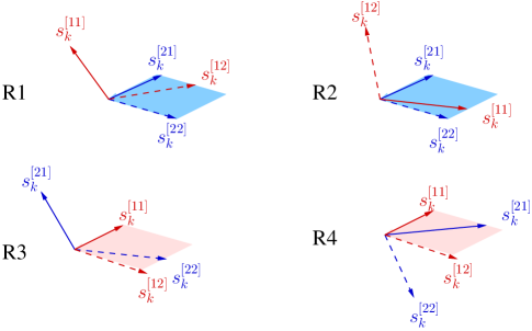
Figure 6: Alignment in the six-dimensional receive signal space. Each arrow represents two dimensions carrying $s_{k}^{[ji]},\ k\in\{1,2\}$. Six interferring symbols are aligned in four-dimensional subspace. The remaining two dimensions are for desired symbols.

From (228), the interfering symbols to Receiver $1$ $\left(c^{[12]}_{1},c^{[12]}_{2},x_{11}^{[2]},x_{12}^{[2]},x^{[2]}_{21},x^{[2]}_{22}\right)$ are aligned in a four-dimensional subspace spanned by the columns of $\mathbf{Q}$. The two desired symbols $c^{[11]}_{1}$ and $c^{[11]}_{2}$ are located in the remaining two-dimensional subspace. The alignment pattern is illustrated in Fig. 6. To cancel the aligned interference, the receiver discards $\tilde{y}^{[11]}_{31}$ and $\tilde{y}^{[11]}_{32}$, then conducts the calculation in (113), i.e.,

$$\left[\begin{array}[]{c}\tilde{y}^{[11]}_{11}+\tilde{y}^{[11]*}_{22}\\ \tilde{y}^{[11]}_{12}-\tilde{y}^{[11]*}_{21}\end{array}\right]=\left[\begin{array}[]{cc}\underline{h}_{11}^{[11]}+\underline{h}^{[11]*}_{22}&\underline{h}_{21}^{[11]}-\underline{h}^{[11]*}_{12}\\ \underline{h}^{[11]}_{12}-\underline{h}^{[11]*}_{21}&\underline{h}^{[11]}_{22}+\underline{h}^{[11]*}_{11}\end{array}\right]\left[\begin{array}[]{c}c^{[11]}_{1}\\ c^{[11]}_{2}\end{array}\right]+\left[\begin{array}[]{c}\tilde{{w}}_{11}^{[11]}+\tilde{{w}}_{22}^{[11]*}\\ \tilde{{w}}_{12}^{[11]}-\tilde{{w}}_{21}^{[11]*}\end{array}\right].$$ (237)

Two desired symbols occupy only a two-dimensional subspace with the equivalent channel matrix having the Alamouti structure. Then, the desired symbols are protected by orthogonal channel vectors due to the Alamouti design.

To summarize the key elements of alignment at Receiver $1$ in Cell $1$, the precoding matrix used in (97) creates an equivalent channel matrix ${\mathcal{H}}^{[12]}$ with the swapped Alamouti structure for the interferring symbol $s^{[12]}_{k}$. Transmitter $2$ aligns to this structure by padding the transmit block $\mathbf{X}^{[2]}$ in time Slot $1$. By using the inversion of the interfering link, six interfering symbols $s^{[12]}_{k}$, $s^{[21]}_{k}$, and $s^{[22]}_{k}$ are able to align in a four-dimensional subspace at both receivers in one cell. It can be verified that such alignment also occurs in Cell $2$. Specifically, alignment is created by the swapped Alamouti structure in time Slots $2$ and $3$ of $\mathbf{X}^{[1]}$.

V Simulation results

In this section, we compare the proposed methods with related transmission schemes in both the short-term regime and the long-term regime. Throughout this section, the horizontal axis in all figures represents SNR measured in dB. Since the noises are normalized and the transmit power of each user is $P$, the SNR of the network is $P$.

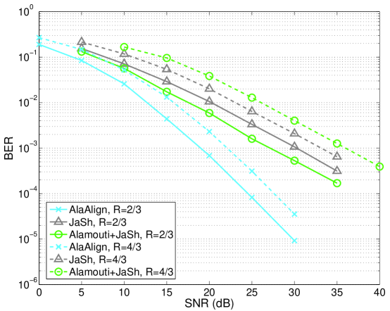
Figure 7: BER comparison in the X channels for the proposed method (labeled as ‘AlaAlign’), the JaSh scheme, and the modified JaSh scheme (labeled as ‘Alamouti+JaSh’). Rate $R$ is measured as bits per channel use per node pair.

Simulations in the short-term regime are performed for two network models. We simulate the average BER performance of the proposed methods. Since the diversity gain is not changed by using any channel codes, we simulate an uncoded system for simplicity. The vertical axis represents the average BER. It is averaged over all communication directions. The first group of simulations shows the BER performance of the proposed alignment method using Alamouti designs in X channels. For comparison, the JaSh scheme[2] is included. In addition, we have a new modified JaSh scheme that has potential for diversity improvement. The modified JaSh scheme uses Alamouti codes on top of the JaSh scheme. Recall that the JaSh scheme creates a $2\times 2$ point-to-point channel after removing the aligned interference and decoupling the symbols from the other transmitter. The modified JaSh scheme uses an Alamouti code for the $2\times 2$ channel to improve diversity while providing only half of the symbol rate of the JaSh scheme. Uncoded symbols $s^{[ji]}_{k}$ are independently generated from a finite constellation. To achieve the same bit rate, different modulations are used for the three methods in Fig. 7. We use BPSK, BPSK, and QPSK modulations for the proposed scheme, the JaSh scheme, and the modified JaSh scheme, respectively, to achieve $2/3$ bits per channel use per pair node (solid curves in Fig. 7). Also, to include comparison at another bit rate, QPSK, QPSK, and 16PSK modulations are used for the proposed scheme, the JaSh scheme, and the modified JaSh scheme, respectively, to achieve $4/3$ bits per channel use per pair node (dashed curves in Fig. 7).

Our proposed method achieves a diversity gain of 2, whereas the JaSh scheme achieves a diversity gain of 1. These results verify the analysis in Subsection III-B. It can be observed that the diversity benefits bring more than $10$ dB gain at BER=$10^{-3}$ for both transmission rates. The modified JaSh scheme cannot bring diversity improvement: only a diversity gain of 1 is observed from Fig. 7. This is because the $2\times 2$ diagonal channel after removing aligned interference and decoupling symbols has correlated diagonal entries. The sum of the achievable SNRs on each channel is upperbounded by a term providing a diversity of only 1. The proof for the diversity gain of the modified JaSh scheme is provided in Appendix C. Consequently, simply using Alamouti codes on top of the JaSh scheme cannot bring diversity improvement.

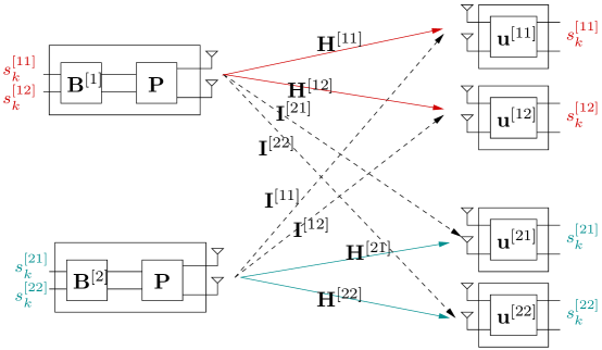
Figure 8: System diagram for the extended downlink interference alignment [18] in the two-user double-antenna IBC.

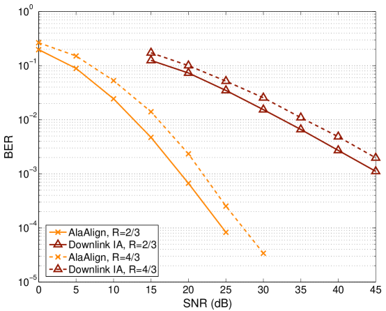
Figure 9: BER comparison in the IBC between the proposed method (labeled as ‘AlaAlign’) and the downlink IA method (labeled as ‘Downlink IA’). Rate $R$ is measured as bits per channel use per receiver.

The second group of simulations compares the extended scheme with the downlink IA [18] in the two-cell IBC. Note that in our setting, each node has two antennas and two symbols are transmitted to each receiver; while in [18], each node has one antenna and one symbol is transmitted to each receiver. We extend the downlink IA method in [18] to our double-antenna setting to achieve the same symbol rate. The system diagram is shown in Fig. 8. The BS uses two transmit precoders: a random precoder $\mathbf{P}$ and a ZF precoder $\mathbf{B}^{[j]}$ to null out intra-cell interference. Each receiver utilizes a receive beamformer $\mathbf{u}^{[ji]}$ to zero-force inter-cell interference. Specifically, the BS sends two symbols to each receiver in three symbol extensions, which creates a six-dimensional signal space. The receive beamformer $\mathbf{u}^{[ji]}\in\mathds{C}^{2\times 6}$ rejects four interferring symbols from the other cell by zero-forcing the equivalent channel matrix $(\mathbf{I}_{3}\otimes\mathbf{I}^{[ji]})\mathbf{P}$ and accepts two desired symbols. The entries in the random precoder $\mathbf{P}\in\mathds{C}^{6\times 4}$ are assumed i. i. d. $\mathcal{CN}(0,1)$ distributed. The ZF precoder $\mathbf{B}\in\mathds{C}^{4\times 4}$ cancels the intra-cell interference by ZF precoding over the equivalent channels $\mathbf{u}^{[ji]}(\mathbf{I}_{3}\otimes\mathbf{I}^{[ji]})\mathbf{P}$. For channel information requirements, both alignment methods need the knowledge of the interferring link at the receivers, and the transmitters require channel information within each cell in addition to the knowledge of the receive beamformers. Since both alignment methods have the same symbol rate, BPSK is used to achieve $2/3$ bits per channel use per receiver (solid curves in Fig. 9), and QPSK is used to achieve $4/3$ bits per channel use per receiver (dashed curves in Fig. 9).

Fig. 9 exhibits the comparison. Our proposed method can achieve a diversity gain of 2, which provides an approximate array gain of $20$ dB at $\mathrm{BER}=10^{-2}$, compared to the downlink IA method.

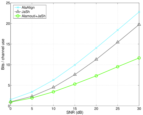
Figure 10: Achievable ergodic mutual information in the two-user X channel.

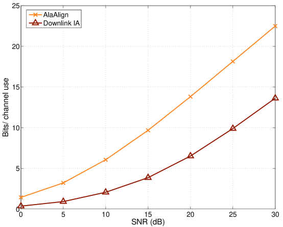
Figure 11: Achievable ergodic mutual information in the two-cell IBC.

In the long-term regime, we simulate and compare the achievable ergodic mutual information for the related methods. An i. i. d. Gaussian codebook is used for each symbol $s_{k}^{[ji]}$. The vertical axis represents the sum rate (measured in bits per channel use) over all communication directions. Figs. 10 and 11 show the ergodic mutual information for the X channel and the IBC, respectively. We can first observe that the proposed method achieves the same DoF gain as the JaSh scheme in Fig. 10, and as the downlink IA method in Fig. 11. Additionally, in the entire SNR regime, our proposed method has a better SNR offset compared to the previous methods. For example, in Fig. 10, the proposed method outperforms the JaSh scheme by approximately $3$ bits/channel use at $\mathrm{SNR}=25$ dB; in Fig. 11, the proposed method enjoys approximately $8$ bits/channel use gain over the downlink IA method at $\mathrm{SNR}=25$ dB. Similar gains are also achieved in the low SNR range. For all compared methods, a ZF receiver is used to cancel the aligned interference as well as decouple the desired signals. Since our proposed method incorporates orthogonal designs between the two symbols from the same user, a ZF receiver does not incur SNR loss when separating these two symbols. On the other hand, for the previous proposed methods, such an SNR loss occurs during the symbol separation. This intuitively explains the SNR gain in the entire SNR range.

VI Conclusions

In this paper, we have proposed a transmission scheme that achieves the maximum symbol-rate, i.e., $\frac{2}{3}$ from node-to-node, with high reliability for the double-antenna $2\times 2$ X channel. The alignment scheme incorporates Alamouti designs before using the normalized inversion of the cross channel as the transmit beamformer to align symbols at unintended receivers. Each receiver removes aligned interference followed by symbol decoupling using IC. Consequently, a symbol-by-symbol decoding complexity is achieved at both receivers. Both simulation and analysis demonstrate a diversity gain of 2 for the symbol-by-symbol decoding in the proposed scheme. This implies that a diversity gain of higher than 1 is achievable in the short-term regime, yet simultaneously with the maximum DoF gain in the long-term regime. The proposed transmission scheme has also been extended to two cellular networks, the IMAC and IBC, to bring the maximum-rate transmission with a diversity gain of 2. Significant BER performance improvement is observed through simulation compared to the downlink IA method. Further extension to the two-user X channels with more than 2 antennas at each node is also doable by sending multiple groups of Alamouti codes for each communication direction.

We have also identified that designing alignment for diversity is not straightforward. Using STBCs on top of the previous alignment method in [2] can neither bring diversity improvements nor maintain the maximum DoF gain for the two-user X channel. This calls for an optimization of existing alignment methods to jointly consider the DoF gain and the diversity gain.

Note that the considered network has 2 antennas at each node. The achievable diversity is upperbounded by the corresponding point-to-point channel. In other words, the maximum diversity gain for the considered network is $2\times 2=4$. Our proposed scheme only achieves the full transmit diversity, whereas the receive diversity gain is only 1. We do not claim that the proposed scheme is optimal in terms of the diversity gain. Since our proposed scheme separates the desired symbols by ZF, it is possible to further improve the receive diversity by a joint-decoding of 4 desired symbols at each receiver. Since the proposed method needs only four symbol-by-symbol decodings, the expense of the joint-decoding algorithm is the increased decoding complexity. We conjecture that such a joint decoding will result in a diversity gain of 4.

To embed Alamouti codes into alignment, the network is required to have infinitely many alignment modes, because Alamouti codes are rotationally invariant. The discussed network models have redundant transmit dimensions. Our design uses a normalized inversion of the cross channels (See Eq.(13)) to constrain the interference subspace to be an identity matrix. In general, the interference subspace can be arbitrarily chosen, thus generating infinitely many alignment modes. Unfortunately, some interference networks, e.g., the interference channels without symbol extensions, have finitely many alignment modes at the maximum DoF gain. Thus, it is not clear how to improve their diversity gains by utilizing orthogonal designs.

Appendix A Two useful lemmas

To prove Theorem 1, we need some lemmas.

Lemma 1

Let the entries of $\mathbf{F}\in\mathds{C}^{2\times 2}$ be i. i. d. $\mathcal{CN}(0,1)$ distributed. The following instantaneous normalized receive SNR

$$\gamma=\frac{1}{{\rm tr}\,\left(\mathbf{F}^{-1}(\mathbf{F}^{-1})^{*}\right)}$$ (238)

provides diversity gain 1.

Proof:

Let the singular values of $\mathbf{F}$ be $\lambda_{1}$ and $\lambda_{2}$ such that $\lambda_{1}\geq\lambda_{2}$. Eqn. (238) can be expanded as

$$\gamma=\frac{1}{{\rm tr}\,\left(\mathbf{F}^{-1}(\mathbf{F}^{-1})^{*}\right)}=\frac{1}{\frac{1}{\lambda_{1}^{2}}+\frac{1}{\lambda_{2}^{2}}}<\frac{1}{\frac{1}{\lambda_{2}^{2}}}=\lambda_{2}^{2}.$$

Since the smaller singular value $\lambda_{2}$ carries diversity 1 only[25], the diversity gain of $\gamma$ is upperbounded by 1. Further, we can lowerbound $\gamma$ as

$$\gamma=\frac{1}{\frac{1}{\lambda_{1}^{2}}+\frac{1}{\lambda_{2}^{2}}}>\frac{1}{\frac{1}{\lambda_{2}^{2}}+\frac{1}{\lambda_{2}^{2}}}=\frac{\lambda_{2}^{2}}{2}.$$

Thus, the instantaneous normalized receive SNR in (238) is lowerbounded by a term with diversity 1. Therefore, the achievable diversity for $\gamma$ is exactly 1. ∎

Lemma 2

Consider the following $N\times 1$ vector system equation

$$\mathbf{y}=\mathbf{h}_{1}s_{1}+\sum_{i=2:M}\mathbf{h}_{i}s_{i}+\mathbf{w},$$ (239)

where $\mathbf{w}\in\mathds{C}^{N\times 1}$ have i. i. d. $\mathcal{CN}(0,1)$ distributed entries, and the channel vectors $\mathbf{h}_{i}\in\mathds{C}^{N\times 1}$ are linearly independent. Let $\mathbf{Q}\in\mathds{C}^{(N-M+1)\times N}$ be any full-rank ZF matrix such that

$$\mathbf{Q}\mathbf{h}_{i}=\mathbf{0}_{N-M+1},\ i\in\{2,\ldots,M\}.$$ (240)

After ZF, the equivalent channel vector is $\mathbf{Q}\mathbf{h}_{1}$ and the noise covariance matrix is $\mathbf{Q}\mathbf{Q}^{*}$. For any designs of $\mathbf{Q}$, the resulting instantaneous normalized receive SNR after ZF is

$$\gamma=\mathbf{h}_{1}^{*}\mathbf{Q}^{*}\left(\mathbf{Q}\mathbf{Q}^{*}\right)^{-1}\mathbf{Q}\mathbf{h}_{1}=\mathbf{h}_{1}^{*}\mathbf{\Sigma}\mathbf{h}_{1},$$ (241)

where $\mathbf{\Sigma}$ is the projection matrix to the null space of $\left[\mathbf{h}_{2},\ldots,\mathbf{h}_{M}\right]$. The instantaneous normalized receive SNR is independent of the designs of $\mathbf{Q}$.

Proof:

Let the SVD of $\mathbf{Q}$ be $\mathbf{Q}=\mathbf{U}\mathbf{\Lambda}\mathbf{V}$ where $\mathbf{U}\in\mathds{C}^{(N-M+1)\times(N-M+1)},\mathbf{V}\in\mathds{C}^{N\times N}$ denote the singular vector matrix and $\mathbf{\Lambda}\in\mathds{C}^{(N-M+1)\times N}$ denotes the singular value matrix. Further denote $\mathbf{\Lambda}=\left[\tilde{\mathbf{\Lambda}}\ \mathbf{0}\right]$ where $\tilde{\mathbf{\Lambda}}\in\mathds{R}^{(N-M+1)\times(N-M+1)}$ denotes the diagonal square matrix with all singular values. It follows

$$\mathbf{Q}^{*}\left(\mathbf{Q}\mathbf{Q}^{*}\right)^{-1}\mathbf{Q} =(\mathbf{U}\mathbf{\Lambda}\mathbf{V})^{*}\left((\mathbf{U}\mathbf{\Lambda}\mathbf{V})(\mathbf{U}\mathbf{\Lambda}\mathbf{V})^{*}\right)^{-1}(\mathbf{U}\mathbf{\Lambda}\mathbf{V})$$

$$=\mathbf{V}^{*}\mathbf{\Lambda}^{*}\mathbf{U}^{*}\left(\mathbf{U}\mathbf{\Lambda}\mathbf{V}\mathbf{V}^{*}\mathbf{\Lambda}^{*}\mathbf{U}^{*}\right)^{-1}\mathbf{U}\mathbf{\Lambda}\mathbf{V}$$

$$=\mathbf{V}^{*}\mathbf{\Lambda}^{*}\mathbf{U}^{*}\left(\mathbf{U}\mathbf{\Lambda}\mathbf{\Lambda}^{*}\mathbf{U}^{*}\right)^{-1}\mathbf{U}\mathbf{\Lambda}\mathbf{V}$$

$$=\mathbf{V}^{*}\mathbf{\Lambda}^{*}\mathbf{U}^{*}\mathbf{U}\left(\mathbf{\Lambda}\mathbf{\Lambda}^{*}\right)^{-1}\mathbf{U}^{*}\mathbf{U}\mathbf{\Lambda}\mathbf{V}$$

$$=\mathbf{V}^{*}\mathbf{\Lambda}^{*}\left(\mathbf{\Lambda}\mathbf{\Lambda}^{*}\right)^{-1}\mathbf{\Lambda}\mathbf{V}=\tilde{\mathbf{V}}^{*}\tilde{\mathbf{\Lambda}}^{*}\left(\tilde{\mathbf{\Lambda}}\tilde{\mathbf{\Lambda}}^{*}\right)^{-1}\tilde{\mathbf{\Lambda}}\tilde{\mathbf{V}}=\tilde{\mathbf{V}}^{*}\tilde{\mathbf{V}},$$

where $\tilde{\mathbf{V}}$ denotes the first $N-M+1$ rows of $\mathbf{V}$. It suffices to verify that $\tilde{\mathbf{V}}^{*}\tilde{\mathbf{V}}$ is the projection matrix to the null space of the subspace spanned by $\left[\mathbf{h}_{2},\ldots,\mathbf{h}_{M}\right]$. For any vector $\hat{\mathbf{h}}\in\mathds{C}^{N\times 1}$ located in the subspace of $\left[\mathbf{h}_{2},\ldots,\mathbf{h}_{M}\right]$, we can assume it to be $\hat{\mathbf{h}}=\underset{i=2:M}{\sum}\mathbf{h}_{i}c_{i}$, where $c_{i}\in\mathds{C}$ is an arbitrary coefficient. From the ZF constraint in (240), we have $\mathbf{Q}\mathbf{h}_{i}=\mathbf{U}\tilde{\mathbf{\Lambda}}\tilde{\mathbf{V}}\mathbf{h}_{i}=\mathbf{0}$. Since $\mathbf{U}$ and $\tilde{\mathbf{\Lambda}}$ are invertible, it follows that $\tilde{\mathbf{V}}\mathbf{h}_{i}=\mathbf{0}$. Thus, we have

$$\tilde{\mathbf{V}}^{*}\tilde{\mathbf{V}}\hat{\mathbf{h}}=\tilde{\mathbf{V}}^{*}\tilde{\mathbf{V}}\underset{i=2:M}{\sum}\mathbf{h}_{i}c_{i}=\underset{i=2:M}{\sum}\tilde{\mathbf{V}}^{*}\left(\tilde{\mathbf{V}}\right)\mathbf{h}_{i}c_{i}=\mathbf{0}.$$

Note that the rows of $\tilde{\mathbf{V}}$ also form an orthonormal basis for the considered null space. Therefore, $\tilde{\mathbf{V}}^{*}\tilde{\mathbf{V}}$ is a projection matrix to the null space of the subspace spanned by $\left[\mathbf{h}_{2},\ldots,\mathbf{h}_{M}\right]$. ∎

Lemma 2 says all ZF receivers are essentially the same in terms of the output SNR. Therefore, to obtain general results for any ZF receivers, we can rely on a special ZF receiver that simplifies the analysis.

Appendix B Proof of Theorem 1

The proof is based on the outage probability of the instantaneous normalized receive SNR $\gamma$ that has been defined in (76). Since the network is statistically symmetric to each symbol, without loss of generality, we only study the expression of $\gamma$ for $s^{[11]}_{k}$. First, we derive $\gamma$ for $s^{[11]}_{k}$. For $M=2$, let the eigenvalues and eigenvectors of $\left(\mathbf{H}^{[11]}\right)^{-1}{\mathbf{H}^{[21]}}\left({\mathbf{H}^{[22]}}\right)^{-1}{\mathbf{H}^{[12]}}$ be $\lambda_{1},\lambda_{2}$ and $\mathbf{u}_{1},\mathbf{u}_{2}$, respectively. The designs in (5) can be expanded as

$$\overline{\mathbf{v}}^{[11]}=\left[\begin{array}[]{cc}\mathbf{u}_{1}&\mathbf{u}_{2}\\ \mathbf{u}_{2}&\mathbf{u}_{1}\\ \mathbf{0}_{2}&\mathbf{0}_{2}\end{array}\right],\ \overline{\mathbf{v}}^{[12]}=\left[\begin{array}[]{cc}\mathbf{u}_{1}&\mathbf{u}_{2}\\ \mathbf{0}_{2}&\mathbf{0}_{2}\\ \mathbf{u}_{2}&\mathbf{u}_{1}\end{array}\right],$$ (248)

where $\mathbf{0}_{2}$ denotes a $2\times 1$ zero vector. The eigenvalues of $\left(\overline{\mathbf{H}}^{[11]}\right)^{-1}{\overline{\mathbf{H}}^{[21]}}\left({\overline{\mathbf{H}}^{[22]}}\right)^{-1}{\overline{\mathbf{H}}^{[12]}}$ are arranged as ${\rm diag}\,\left(\lambda_{1},\lambda_{2},\lambda_{2},\lambda_{2},\lambda_{1},\lambda_{1}\right)$. Inserting the designs of transmit beamformers in (4) into (2) gives the received signals at Receiver $1$

$$\mathbf{y}^{[1]} =\overline{\mathbf{H}}^{[11]}\overline{\mathbf{v}}^{[11]}\left[\begin{array}[]{c}s^{[11]}_{1}\\ s^{[11]}_{2}\end{array}\right]+\overline{\mathbf{H}}^{[21]}\overline{\mathbf{v}}^{[21]}\left[\begin{array}[]{c}s^{[21]}_{1}\\ s^{[21]}_{2}\end{array}\right]+\overline{\mathbf{H}}^{[11]}\overline{\mathbf{v}}^{[12]}\left[\begin{array}[]{c}s^{[12]}_{1}\\ s^{[12]}_{2}\end{array}\right]+\overline{\mathbf{H}}^{[21]}\overline{\mathbf{v}}^{[22]}\left[\begin{array}[]{c}s^{[22]}_{1}\\ s^{[22]}_{2}\end{array}\right]+\mathbf{w}^{[1]}$$ (257)

$$=\overline{\mathbf{H}}^{[11]}\overline{\mathbf{v}}^{[11]}\left[\begin{array}[]{c}s^{[11]}_{1}\\ s^{[11]}_{2}\end{array}\right]+\alpha^{[21]}\overline{\mathcal{H}}^{[21]}\overline{\mathbf{v}}^{[11]}\left[\begin{array}[]{c}s^{[21]}_{1}\\ s^{[21]}_{2}\end{array}\right]+\overline{\mathbf{H}}^{[11]}\overline{\mathbf{v}}^{[12]}\left[\begin{array}[]{c}s^{[12]}_{1}\\ s^{[12]}_{2}\end{array}\right]+\alpha^{[22]}\overline{\mathbf{H}}^{[11]}\overline{\mathbf{v}}^{[12]}\left[\begin{array}[]{c}s^{[22]}_{1}\\ s^{[22]}_{2}\end{array}\right]+\mathbf{w}^{[1]}$$ (266)

$$=\overline{\mathbf{H}}^{[11]}\overline{\mathbf{v}}^{[11]}\left[\begin{array}[]{c}s^{[11]}_{1}\\ s^{[11]}_{2}\end{array}\right]+\alpha^{[21]}\overline{\mathcal{H}}^{[21]}\overline{\mathbf{v}}^{[11]}\left[\begin{array}[]{c}s^{[21]}_{1}\\ s^{[21]}_{2}\end{array}\right]+\overline{\mathbf{H}}^{[11]}\overline{\mathbf{v}}^{[12]}\underset{\left[I_{1}\ I_{2}\right]^{\mathrm{T}}}{\underbrace{\left[\begin{array}[]{c}s^{[12]}_{1}+\alpha^{[22]}s^{[22]}_{1}\\ s^{[12]}_{2}+\alpha^{[22]}s^{[22]}_{2}\end{array}\right]}}+\mathbf{w}^{[1]},$$ (273)

where $\overline{\mathcal{H}}^{[21]}=\overline{\mathbf{H}}^{[21]}\left(\overline{\mathbf{H}}^{[22]}\right)^{-1}\overline{\mathbf{H}}^{[12]}$; $I_{1},I_{2}$ denote the aligned interference; and $\alpha^{[21]},\alpha^{[22]}$ are coefficients to normalize the power of transmit beamformers. Note that $\left(\mathbf{H}^{[11]}\right)^{-1}\mathbf{H}^{[21]}\left(\mathbf{H}^{[22]}\right)^{-1}\mathbf{H}^{[12]}\mathbf{u}_{i}=\lambda_{i}\mathbf{u}_{i}$ due to the definition of eigenvalue decomposition. Let ${\mathcal{H}}^{[21]}={\mathbf{H}}^{[21]}\left({\mathbf{H}}^{[22]}\right)^{-1}{\mathbf{H}}^{[12]}$. It follows ${\mathcal{H}}^{[21]}\mathbf{u}_{i}=\lambda_{i}\mathbf{H}^{[11]}\mathbf{u}_{i}$.

Replacing the designs in (248) into (273) gives

$$\mathbf{y}^{[1]}=\overline{\mathbf{H}}^{[11]}\left[\begin{array}[]{cc}\mathbf{u}_{1}&\mathbf{u}_{2}\\ \mathbf{u}_{2}&\mathbf{u}_{1}\\ \mathbf{0}_{2}&\mathbf{0}_{2}\end{array}\right]\left[\begin{array}[]{c}s^{[11]}_{1}\\ s^{[11]}_{2}\end{array}\right]+\alpha^{[21]}(\mathbf{I}_{3}\otimes\mathcal{H}^{[21]})\left[\begin{array}[]{cc}\mathbf{u}_{1}&\mathbf{u}_{2}\\ \mathbf{u}_{2}&\mathbf{u}_{1}\\ \mathbf{0}_{2}&\mathbf{0}_{2}\end{array}\right]\left[\begin{array}[]{c}s^{[21]}_{1}\\ s^{[21]}_{2}\end{array}\right]+\overline{\mathbf{H}}^{[11]}\left[\begin{array}[]{cc}\mathbf{u}_{1}&\mathbf{u}_{2}\\ \mathbf{0}_{2}&\mathbf{0}_{2}\\ \mathbf{u}_{2}&\mathbf{u}_{1}\end{array}\right]\left[\begin{array}[]{c}I_{1}\\ I_{2}\end{array}\right]+\mathbf{w}^{[1]}$$ (289)

$$=\overline{\mathbf{H}}^{[11]}\left[\begin{array}[]{cc}\mathbf{u}_{1}&\mathbf{u}_{2}\\ \mathbf{u}_{2}&\mathbf{u}_{1}\\ \mathbf{0}_{2}&\mathbf{0}_{2}\end{array}\right]\left[\begin{array}[]{c}s^{[11]}_{1}\\ s^{[11]}_{2}\end{array}\right]+\alpha^{[21]}\overline{\mathbf{H}}^{[11]}\left[\begin{array}[]{cc}\lambda_{1}\mathbf{u}_{1}&\lambda_{2}\mathbf{u}_{2}\\ \lambda_{2}\mathbf{u}_{2}&\lambda_{1}\mathbf{u}_{1}\\ \mathbf{0}_{2}&\mathbf{0}_{2}\end{array}\right]\left[\begin{array}[]{c}s^{[21]}_{1}\\ s^{[21]}_{2}\end{array}\right]+\overline{\mathbf{H}}^{[11]}\left[\begin{array}[]{cc}\mathbf{u}_{1}&\mathbf{u}_{2}\\ \mathbf{0}_{2}&\mathbf{0}_{2}\\ \mathbf{u}_{2}&\mathbf{u}_{1}\end{array}\right]\left[\begin{array}[]{c}I_{1}\\ I_{2}\end{array}\right]+\mathbf{w}^{[1]}.$$ (305)

To decouple $s^{[11]}_{1}$, the receiver projects $\mathbf{y}^{[1]}$ into the null of the subspaces spanned by the equivalent channel vectors of $s^{[11]}_{2},s^{[21]}_{1},s^{[21]}_{2},I_{1}$, and $I_{2}$. The resulting instantaneous normalized receive SNR $\gamma$ is upperbounded by that of the scenario when projecting only the null of the subspace spanned by $s^{[11]}_{2},s^{[21]}_{1}$, and $s^{[21]}_{2}$. This upperbound system corresponds to the system equation without aligned interference

$$\left[\begin{array}[]{c}\tilde{\mathbf{y}}_{1}^{[1]}\\ \tilde{\mathbf{y}}_{2}^{[1]}\end{array}\right]=\left[\begin{array}[]{cc}{\mathbf{H}}^{[11]}&\\ &\mathbf{H}^{[11]}\end{array}\right]\left[\begin{array}[]{cc}\mathbf{u}_{1}&\mathbf{u}_{2}\\ \mathbf{u}_{2}&\mathbf{u}_{1}\end{array}\right]\left[\begin{array}[]{c}s^{[11]}_{1}\\ s^{[11]}_{2}\end{array}\right]+\alpha^{[21]}\left[\begin{array}[]{cc}\mathbf{H}^{[11]}&\\ &\mathbf{H}^{[11]}\end{array}\right]\left[\begin{array}[]{cc}\lambda_{1}\mathbf{u}_{1}&\lambda_{2}\mathbf{u}_{2}\\ \lambda_{2}\mathbf{u}_{2}&\lambda_{1}\mathbf{u}_{1}\end{array}\right]\left[\begin{array}[]{c}s^{[21]}_{1}\\ s^{[21]}_{2}\end{array}\right]+\left[\begin{array}[]{c}\tilde{\mathbf{w}}^{[1]}_{1}\\ \tilde{\mathbf{w}}^{[1]}_{2}\end{array}\right],$$ (322)

where $\left[\tilde{\mathbf{y}}^{[1]\mathrm{T}}_{1},\tilde{\mathbf{y}}^{[1]\mathrm{T}}_{2}\right]^{\mathrm{T}}$ corresponds to the first four entries in $\mathbf{y}^{[1]}$ with $\tilde{\mathbf{y}}^{[1]}_{1},\tilde{\mathbf{y}}^{[1]}_{2}\in\mathds{C}^{2\times 1}$, and similar notations apply to $\tilde{\mathbf{w}}^{[1]}_{1},\tilde{\mathbf{w}}^{[1]}_{2}\in\mathds{C}^{2\times 1}$. To simplify the analysis, from Lemma 2, we can use a specific ZF receiver that does not lose generality. We first invert the channel matrix $\mathbf{H}^{[11]}$ and switch the positions of $s_{2}^{[11]}$ and $s_{2}^{[21]}$ as

$$\left[\begin{array}[]{c}\left({\mathbf{H}}^{[11]}\right)^{-1}\tilde{\mathbf{y}}_{1}^{[1]}\\ \left({\mathbf{H}}^{[11]}\right)^{-1}\tilde{\mathbf{y}}_{2}^{[1]}\end{array}\right] =\left[\begin{array}[]{cc}\mathbf{u}_{1}&\mathbf{u}_{2}\\ \mathbf{u}_{2}&\kappa\mathbf{u}_{1}\end{array}\right]\left[\begin{array}[]{c}s^{[11]}_{1}\\ \alpha^{[21]}\lambda_{2}s^{[21]}_{2}\end{array}\right]$$ (329)

$$+\left[\begin{array}[]{cc}\kappa\mathbf{u}_{1}&\mathbf{u}_{2}\\ \mathbf{u}_{2}&\mathbf{u}_{1}\end{array}\right]\left[\begin{array}[]{c}\alpha^{[21]}\lambda_{2}s^{[21]}_{1}\\ s^{[11]}_{2}\end{array}\right]+\left[\begin{array}[]{c}\left({\mathbf{H}}^{[11]}\right)^{-1}\tilde{\mathbf{w}}^{[1]}_{1}\\ \left({\mathbf{H}}^{[11]}\right)^{-1}\tilde{\mathbf{w}}^{[1]}_{2}\end{array}\right],$$ (336)

where $\kappa$ denotes the ratio of the eigenvalues of $\left(\mathbf{H}^{[11]}\right)^{-1}{\mathbf{H}^{[21]}}\left({\mathbf{H}^{[22]}}\right)^{-1}{\mathbf{H}^{[12]}}$, i.e., $\kappa=\frac{\lambda_{1}}{\lambda_{2}}$. Define $\mathbf{u}=\left[\mathbf{u}_{1}\ \mathbf{u}_{2}\right]$ as the eigenvector matrix of $\left(\mathbf{H}^{[11]}\right)^{-1}{\mathbf{H}^{[21]}}\left({\mathbf{H}^{[22]}}\right)^{-1}{\mathbf{H}^{[12]}}$ and

$$\mathbf{P}=\left[\begin{array}[]{cc}0&1\\ 1&0\end{array}\right],\mathbf{Q}=\left[\begin{array}[]{cc}\kappa&0\\ 0&1\end{array}\right].$$ (341)

To cancel $s^{[21]}_{1}$ and $s^{[11]}_{2}$, the receiver calculates $\tilde{\mathbf{y}}\in\mathds{C}^{2\times 1}$ as

$$\tilde{\mathbf{y}}=(\mathbf{H}^{[11]})^{-1}\tilde{\mathbf{y}}^{[1]}_{1}-\mathbf{u}\mathbf{Q}(\mathbf{H}^{[11]}\mathbf{u}\mathbf{P})^{-1}\tilde{\mathbf{y}}^{[1]}_{2}=\left(\mathbf{u}-\mathbf{u}\mathbf{Q}\left(\mathbf{u}\mathbf{P}\right)^{-1}\mathbf{u}\mathbf{Q}\mathbf{P}\right)\left[\begin{array}[]{cc}s^{[11]}_{1}&\alpha^{[21]}\lambda_{2}s^{[21]}_{2}\end{array}\right]^{\mathrm{T}}$$ (343)

$$+(\mathbf{H}^{[11]})^{-1}\tilde{\mathbf{w}}^{[1]}_{1}-\mathbf{u}(\mathbf{Q}\mathbf{P}^{-1})\mathbf{u}^{-1}\left(\mathbf{H}^{[11]}\right)^{-1}\tilde{\mathbf{w}}^{[1]}_{2}$$

$$=(1-\kappa)\mathbf{u}\left[\begin{array}[]{cc}s^{[11]}_{1}&\alpha^{[21]}\lambda_{2}s^{[21]}_{2}\end{array}\right]^{\mathrm{T}}+(\mathbf{H}^{[11]})^{-1}\tilde{\mathbf{w}}^{[1]}_{1}-\mathbf{u}\mathbf{Q}\mathbf{P}\mathbf{u}^{-1}(\mathbf{H}^{[11]})^{-1}\tilde{\mathbf{w}}^{[1]}_{2}.$$ (345)

Note that the equivalent channel matrix is $\mathbf{u}$. To further decouple $s^{[11]}_{1}$ from $s^{[21]}_{2}$ by ZF, the receiver multiplies $\mathbf{u}^{-1}$ to the left side of $\tilde{\mathbf{y}}$ to achieve

$$\mathbf{u}^{-1}\tilde{\mathbf{y}}=(1-\kappa)\left[\begin{array}[]{cc}s^{[11]}_{1}&\alpha^{[21]}\lambda_{2}s^{[21]}_{2}\end{array}\right]^{\mathrm{T}}+\underset{\tilde{\mathbf{w}}}{\underbrace{\mathbf{u}^{-1}(\mathbf{H}^{[11]})^{-1}\tilde{\mathbf{w}}^{[1]}_{1}-\mathbf{Q}\mathbf{P}\mathbf{u}^{-1}(\mathbf{H}^{[11]})^{-1}\tilde{\mathbf{w}}^{[1]}_{2}}}.$$ (347)

Since the entries in $\tilde{\mathbf{w}}^{[1]}_{1}$ and $\tilde{\mathbf{w}}^{[1]}_{2}$ are i. i. d. $\mathcal{CN}(0,1)$ distributed, the covariance matrix of the equivalent noise vector $\tilde{\mathbf{w}}$ can be calculated as

$$\mathbf{\Sigma}=\mathbf{u}^{-1}\left(\mathbf{H}^{[11]*}\mathbf{H}^{[11]}\right)^{-1}(\mathbf{u}^{-1})^{*}+\mathbf{Q}\mathbf{P}\mathbf{u}^{-1}\left(\mathbf{H}^{[11]*}\mathbf{H}^{[11]}\right)^{-1}(\mathbf{u}^{-1})^{*}\mathbf{P}\mathbf{Q}.$$ (348)

To decode $s^{[11]}_{1}$, the receiver uses the $(1,1)$th entry of $\mathbf{\Sigma}$ as the variance for noise. Denote

$$\mathbf{\Delta}=\left(\mathbf{u}^{*}\mathbf{H}^{[11]*}\mathbf{H}^{[11]}\mathbf{u}\right)^{-1}$$ (349)

and its $(i,j)$th entry as $\delta_{ij}$. The noise variance in the decoding of $s^{[11]}_{1}$ can be calculated as $\delta_{11}+\kappa^{2}\delta_{22}$. The instantaneous normalized receive SNR for this upperbound system can be expressed as

$$\gamma^{\prime}=\frac{(1-\kappa)^{2}}{\delta_{11}+\kappa^{2}\delta_{22}}.$$ (350)

Now, we focus on the outage probability of $\gamma$. Let $\epsilon$ be an arbitrary small positive number. The outage probability of the upperbound system can be expanded as

$$P(\gamma<\epsilon)>P(\gamma^{\prime}<\epsilon)>P(\gamma^{\prime}<\epsilon|1\leq|\kappa|\leq 2)P(1\leq|\kappa|\leq 2).$$ (351)

Using the condition $1\leq|\kappa|\leq 2$, we can further upperbound $\gamma^{\prime}$ by $\gamma^{\prime}<\frac{(1+2)^{2}}{\delta_{11}+\delta_{22}}=\frac{9}{{\rm tr}\,\mathbf{\Delta}}$. Thus, we have

$$P(\gamma<\epsilon)>P\left(\frac{1}{{\rm tr}\,\mathbf{\Delta}}<\frac{\epsilon}{9}\right)P(1\leq|\kappa|\leq 2).$$

Recall that $\kappa$ is the ratio of the eigenvalues of $\left(\mathbf{H}^{[11]}\right)^{-1}{\mathbf{H}^{[21]}}\left({\mathbf{H}^{[22]}}\right)^{-1}{\mathbf{H}^{[12]}}$. All channel matrices are independently generated from a continuous distribution. Thus, $P(1\leq|\kappa|\leq 2)$ is a bounded nonzero positive number. It suffices to rely on the scaling of the outage probability of $\frac{1}{{\rm tr}\,\mathbf{\Delta}}$. From the definition of $\mathbf{\Delta}$ in (349), we have

$$\frac{1}{{\rm tr}\,\mathbf{\Delta}}=\frac{1}{{\rm tr}\,\left(\left(\mathbf{u}^{*}\mathbf{H}^{[11]*}\mathbf{H}^{[11]}\mathbf{u}\right)^{-1}\right)}=\frac{1}{{\rm tr}\,\left((\mathbf{H}^{[11]*}\mathbf{H}^{[11]})^{-1}\left(\mathbf{u}\mathbf{u}^{*}\right)^{-1}\right)}<\frac{2}{{\rm tr}\,\left((\mathbf{H}^{[11]*}\mathbf{H}^{[11]})^{-1}\right)}.$$

The inequality in the last line is valid because $\mathbf{u}\mathbf{u}^{*}\prec{\rm tr}\,(\mathbf{u}\mathbf{u}^{*})\mathbf{I}_{2}=2\mathbf{I}_{2}$, where ${\rm tr}\,(\mathbf{u}\mathbf{u}^{*})\mathbf{I}_{2}-\mathbf{u}\mathbf{u}^{*}$ is a positive definite matrix. Applying Lemma 1 to the term $\frac{1}{{\rm tr}\,\left((\mathbf{H}^{[11]})^{-1}(\mathbf{H}^{[11]*})^{-1}\right)}$ results in a diversity gain of only 1. Thus, the achievable diversity for $\frac{1}{{\rm tr}\,\mathbf{\Delta}}$ is not larger than 1. This concludes the proof.

Appendix C Diversity analysis for the modified JaSh scheme

The modified JaSh scheme collects two alignment blocks and uses Alamouti codes as the inner codes. The resulting instantaneous normalized receive SNR is the sum of those of $s_{1}^{[11]}$ and $s_{2}^{[11]}$ in the JaSh scheme. In this appendix, we present the analysis for the modified JaSh scheme.

Theorem 5

In the short-term regime, the achievable diversity gain of the modified JaSh scheme is no more than 1 for the $2\times 2$ double-antenna X channel.

Proof:

The analysis is similar to the proof of Theorem 1. From (305), the instantaneous normalized receive SNR of $s_{2}^{[11]}$ can be obtained from that of $s_{1}^{[11]}$ by swapping $\mathbf{u}_{1}$ and $\mathbf{u}_{2}$. Similar to the specific ZF receiver in (345) and (347), we can obtain an upperbound on the instantaneous normalized receive SNR of $s_{2}^{[11]}$ from (350) as

$$\gamma_{2}^{[11]}<\frac{(1-\kappa)^{2}}{\kappa^{2}\delta_{11}+\delta_{22}},$$

where $\kappa$ and $\delta_{ij}$ are defined in (336) and (349), respectively. Since the use of Alamouti codes accumulates the SNRs of $s_{1}^{[11]}$ and $s_{2}^{[11]}$, we have

$$\gamma_{1}^{[11]}+\gamma_{2}^{[11]}<\frac{(1-\kappa)^{2}}{\delta_{11}+\kappa^{2}\delta_{22}}+\frac{(1-\kappa)^{2}}{\kappa^{2}\delta_{11}+\delta_{22}}.$$

The conditional bounding technique in (351) can be straightforwardly applied as

$$P\left(\gamma_{1}^{[11]}+\gamma_{2}^{[11]}<\epsilon\right)>P\left(\frac{(1-\kappa)^{2}}{\delta_{11}+\kappa^{2}\delta_{22}}+\frac{(1-\kappa)^{2}}{\kappa^{2}\delta_{11}+\delta_{22}}<\epsilon\mid 1\leq|\kappa|\leq 2\right)P(1\leq|\kappa|\leq 2)$$

$$>P\left(\frac{1}{\delta_{11}+\delta_{22}}<\frac{\epsilon}{18}\right)P(1\leq|\kappa|\leq 2).$$

The rest of the proof is similar to that of Theorem 1 by showing that the scaling of the outage probability of $P\left(\frac{1}{\delta_{11}+\delta_{22}}<\epsilon\right)$ has only diversity 1. This concludes the proof. ∎

The results of Theorem 5 are surprising. Although the instantaneous normalized receive SNRs $\gamma_{1}^{[11]}$ and $\gamma_{2}^{[11]}$ are correlated, they are still distinct. Theorem 5 implies that the sum of two distinct SNRs is not sufficient to achieve a diversity of 2.

Appendix D Proof of Theorem 3

The proof is based on the outage probability of the instantaneous normalized receive SNR of $s_{1}^{[11]}$. Since the design is symmetric for all symbols, similar diversity results apply to the decoding of other symbols. Let $\hat{\mathbf{H}}^{[21]}=\left[\frac{\hat{\mathbf{H}}_{1}^{[21]*}}{\left\|\hat{\mathbf{H}}^{[21]}_{1}\right\|^{2}}\ -\frac{\hat{\mathbf{H}}_{2}^{[21]*}}{\left\|\hat{\mathbf{H}}_{2}^{[21]}\right\|^{2}}\right]^{*}$, $\hat{\mathbf{H}}^{[11]}=\left[\hat{\mathbf{H}}_{1}^{[11]*}\ \hat{\mathbf{H}}_{2}^{[11]*}\right]^{*}$. The equivalent system in (74) can be rewritten as

$$\hat{\mathbf{y}}=\sqrt{\frac{3}{4}}\hat{\mathbf{H}}^{[21]*}\hat{\mathbf{H}}^{[11]}\left[\begin{array}[]{c}s^{[11]}_{1}\\ s^{[11]}_{2}\end{array}\right]+\hat{\mathbf{H}}^{[21]*}\left[\begin{array}[]{c}\hat{\mathbf{w}}_{1}\\ \hat{\mathbf{w}}_{2}\end{array}\right].$$ (356)

The covariance matrix of the equivalent noise vector is $\hat{\mathbf{H}}^{[21]*}\mathbf{\Sigma}_{\hat{\mathbf{w}}}\hat{\mathbf{H}}^{[21]}$, where $\mathbf{\Sigma}_{\hat{\mathbf{w}}}={\rm diag}\,\left(1,2,1,2\right).$ Let the first column of $\hat{\mathbf{H}}^{[11]}$ be $\hat{\mathbf{h}}_{1}^{[11]}$, where $\hat{\mathbf{h}}_{1}^{[11]}=\left[\tilde{h}_{11}^{[11]}\ \tilde{h}_{21}^{[11]*}\ \tilde{h}_{12}^{[11]}\ \tilde{h}_{22}^{[11]*}\right]^{\mathrm{T}}$. The instantaneous normalized receive SNR of $s_{1}^{[11]}$ can be expressed as

$$\gamma=\frac{3}{4}\left(\hat{\mathbf{H}}^{[21]*}\hat{\mathbf{h}}^{[11]}_{1}\right)^{*}\left(\hat{\mathbf{H}}^{[21]*}\mathbf{\Sigma}_{\hat{\mathbf{w}}}\hat{\mathbf{H}}^{[21]}\right)^{-1}\hat{\mathbf{H}}^{[21]*}\hat{\mathbf{h}}^{[11]}_{1}.$$

Define $\bar{\gamma}=\hat{\mathbf{h}}_{1}^{[11]*}\hat{\mathbf{H}}^{[21]}\left(\hat{\mathbf{H}}^{[21]*}\hat{\mathbf{H}}^{[21]}\right)^{-1}\hat{\mathbf{H}}^{[21]*}\hat{\mathbf{h}}^{[11]}_{1}$. It can be shown that $\frac{3}{4}\bar{\gamma}\geq\gamma\geq\frac{3}{8}\bar{\gamma}$. By (76), $\gamma$ and $\bar{\gamma}$ have the same diversity. Thus, we focus on analyzing the outage probability of $\bar{\gamma}$ to get rid of $\mathbf{\Sigma}_{\hat{\mathbf{w}}}$. Since the columns of $\hat{\mathbf{H}}^{[21]}$ are orthogonal, $\bar{\gamma}$ can be further simplified as

$$\bar{\gamma}=\underset{b^{[21]}}{\underbrace{\left(\frac{1}{2\left\|\hat{\mathbf{H}}^{[21]}_{1}\right\|^{2}}+\frac{1}{2\left\|\hat{\mathbf{H}}^{[21]}_{2}\right\|^{2}}\right)^{-1}}}\hat{\mathbf{h}}_{1}^{[11]*}\hat{\mathbf{H}}^{[21]}\hat{\mathbf{H}}^{[21]*}\hat{\mathbf{h}}^{[11]}_{1}.$$ (357)

It is complicated to analyze the distribution of $\bar{\gamma}$ directly. Instead, we fix $\mathbf{H}^{[21]}$, $\mathbf{H}^{[12]}$, and $\mathbf{H}^{[22]}$, and allow only $\mathbf{H}^{[11]}$ to change. Then, $\hat{\mathbf{H}}^{[21]}$ is fixed, whereas $\hat{\mathbf{h}}_{1}^{[11]}$ is still a random vector. Since $\tilde{\mathbf{H}}^{[11]}=\frac{1}{\left\|(\mathbf{H}^{[12]})^{-1}\right\|}(\mathbf{H}^{[12]})^{-1}\mathbf{H}^{[11]}$, it can be shown that the conditional distribution of $\bar{\gamma}$ is a generalized Chi-square distribution with degree 2. The covariance matrix of the components in the generalized Chi-square distribution can be calculated as

$$\mathbf{\Phi}=\underset{\mathbf{H}^{[11]}|\mathbf{H}^{[ji]},(j,i)\neq(1,1)}{{\mathbb{E}}\,}b^{[21]}\hat{\mathbf{H}}^{[21]*}\hat{\mathbf{h}}^{[11]}_{1}\hat{\mathbf{h}}^{[11]*}_{1}\hat{\mathbf{H}}^{[21]}=b^{[21]}\hat{\mathbf{H}}^{[21]*}\left(\underset{\mathbf{H}^{[11]}|\mathbf{H}^{[ji]},(j,i)\neq(1,1)}{{\mathbb{E}}\,}\left(\hat{\mathbf{h}}^{[11]}_{1}\hat{\mathbf{h}}_{1}^{[11]*}\right)\right)\hat{\mathbf{H}}^{[21]}.$$ (358)

The equality holds because $\hat{\mathbf{H}}^{[21]}$ only depends on $\tilde{\mathbf{H}}^{[21]}$, which depends on $\mathbf{H}^{[21]}$ and $\mathbf{H}^{[22]}$. Thus, $\hat{\mathbf{H}}^{[21]}$ is independent from $\mathbf{H}^{[11]}$. It can be calculated that ${\mathbb{E}}\,\left(\tilde{h}^{[11]}_{1i}\tilde{h}_{1i}^{[11]*}\right)=\frac{\left\|\left(\mathbf{H}^{[12]}\right)^{-1}_{1\cdot}\right\|^{2}}{\left\|\left(\mathbf{H}^{[12]}\right)^{-1}\right\|^{2}}$, ${\mathbb{E}}\,\left(\tilde{h}^{[11]}_{2i}\tilde{h}_{2i}^{[11]*}\right)=\frac{\left\|\left(\mathbf{H}^{[12]}\right)^{-1}_{2\cdot}\right\|^{2}}{\left\|\left(\mathbf{H}^{[12]}\right)^{-1}\right\|^{2}}$, and ${\mathbb{E}}\,\left(\tilde{h}^{[11]}_{1i}\tilde{h}^{[11]}_{2i}\right)=0$ for $i=1,2$, where $\left(\mathbf{H}^{[12]}\right)^{-1}_{k\cdot}$ denotes the $k$th row of $\left(\mathbf{H}^{[12]}\right)^{-1}$. Let $\mathbf{\Theta}_{\mathbf{H}^{[12]}}={\rm diag}\,\left(\frac{\left\|\left(\mathbf{H}^{[12]}\right)^{-1}_{1\cdot}\right\|^{2}}{\left\|\left(\mathbf{H}^{[12]}\right)^{-1}\right\|^{2}},\frac{\left\|\left(\mathbf{H}^{[12]}\right)^{-1}_{2\cdot}\right\|^{2}}{\left\|\left(\mathbf{H}^{[12]}\right)^{-1}\right\|^{2}}\right)$. The covariance matrix can be simplified as

$$\mathbf{\Phi}=b^{[21]}\left(\frac{\hat{\mathbf{H}}^{[21]*}_{1}\mathbf{\Theta}_{\mathbf{H}^{[12]}}\hat{\mathbf{H}}^{[21]}_{1}}{\left\|\hat{\mathbf{H}}^{[21]}_{1}\right\|^{4}}+\frac{\hat{\mathbf{H}}_{2}^{[21]*}\mathbf{\Theta}_{\mathbf{H}^{[12]}}\hat{\mathbf{H}}_{2}^{[21]}}{\left\|\hat{\mathbf{H}}^{[21]}_{2}\right\|^{4}}\right).$$ (359)

Given the covariance matrix, we calculate the outage probability of $\bar{\gamma}$ conditioned on $\mathbf{H}^{[21]}$, $\mathbf{H}^{[12]}$, and $\mathbf{H}^{[22]}$. Denote the eigenvalues of $\mathbf{\Phi}$ as $\lambda_{1}$ and $\lambda_{2}$. Since the distribution of $\bar{\gamma}$ is a generalized Chi-square with degree 2, the probability density function (pdf) of $\bar{\gamma}$ is $f_{\bar{\gamma}}=\frac{\exp\left(-\bar{\gamma}/\lambda_{1}\right)}{\lambda_{1}-\lambda_{2}}+\frac{\exp\left(-\bar{\gamma}/\lambda_{2}\right)}{\lambda_{2}-\lambda_{1}}$. It follows that

$$P\left(\bar{\gamma}<\epsilon|\mathbf{H}^{[21]},\mathbf{H}^{[12]},\mathbf{H}^{[22]}\right)=\int_{0}^{\epsilon}\frac{\exp\left(-\frac{\bar{\gamma}}{\lambda_{1}}\right)}{\lambda_{1}-\lambda_{2}}+\frac{\exp\left(-\frac{\bar{\gamma}}{\lambda_{2}}\right)}{\lambda_{2}-\lambda_{1}}d\bar{\lambda}$$

$$=\frac{\lambda_{1}}{\lambda_{1}-\lambda_{2}}\left(1-\exp\left(-\frac{\epsilon}{\lambda_{1}}\right)\right)-\frac{\lambda_{2}}{\lambda_{1}-\lambda_{2}}\left(1-\exp\left(-\frac{\epsilon}{\lambda_{2}}\right)\right)$$

$$=1-\frac{\lambda_{1}}{\lambda_{1}-\lambda_{2}}\exp\left(-\frac{\epsilon}{\lambda_{1}}\right)+\frac{\lambda_{2}}{\lambda_{1}-\lambda_{2}}\exp\left(-\frac{\epsilon}{\lambda_{2}}\right)$$

$$=1-\frac{\lambda_{1}}{\lambda_{1}-\lambda_{2}}\left(1-\frac{\epsilon}{\lambda_{1}}+\frac{\epsilon^{2}}{\lambda_{1}^{2}}\right)+\frac{\lambda_{2}}{\lambda_{1}-\lambda_{2}}\left(1-\frac{\epsilon}{\lambda_{2}}+\frac{\epsilon^{2}}{\lambda_{2}^{2}}\right)+o\left(\epsilon^{2}\right)=\frac{\epsilon^{2}}{\lambda_{1}\lambda_{2}}+o\left(\epsilon^{2}\right).$$

Using (76), the diversity gain of $\bar{\gamma}$ can be calculated as

$$d=\lim_{\epsilon\rightarrow 0}\frac{\log P(\gamma<\epsilon)}{\log\epsilon}=\lim_{\epsilon\rightarrow 0}\frac{\log\underset{\mathbf{H}^{[ji]},(j,i)\neq(1,1)}{{\mathbb{E}}\,}P\left(\gamma<\epsilon|\mathbf{H}^{[ji]},(j,i)\neq(1,1)\right)}{\log\epsilon}$$

$$=\lim_{\epsilon\rightarrow 0}\frac{\log\epsilon^{2}\left(\underset{\mathbf{H}^{[ji]}}{{\mathbb{E}}\,}\frac{1}{\lambda_{1}\lambda_{2}}\right)+o(\epsilon^{2})}{\log\epsilon}.$$

Obviously, the achievable diversity gain is 2 if and only if $\underset{\mathbf{H}^{[ji]}}{{\mathbb{E}}\,}\frac{1}{\lambda_{1}\lambda_{2}}$ is bounded by a limited number. Next, we show that $\underset{\mathbf{H}^{[ji]}}{{\mathbb{E}}\,}\frac{1}{\lambda_{1}\lambda_{2}}$ is upperbounded by a limited number, followed by being lowerbounded by another number.

Theorem VI.7.1 in [26] introduces a lowerbound on the determinant of the sum of two Hermitian matrices. Since $\mathbf{\Theta}_{\mathbf{H}^{[12]}}$ is a diagonal matrix, we have $\det\mathbf{\Phi}>\det\mathbf{\Theta}_{\mathbf{H}^{[12]}}$. It follows,

$$\underset{\mathbf{H}^{[ji]}}{{\mathbb{E}}\,}\frac{1}{\lambda_{1}\lambda_{2}}=\underset{\mathbf{H}^{[ji]}}{{\mathbb{E}}\,}\frac{1}{\det\mathbf{\Phi}}<\underset{\mathbf{H}^{[12]}}{{\mathbb{E}}\,}\frac{1}{\det\mathbf{\Theta}_{\mathbf{H}^{[12]}}}<\underset{\mathbf{H}^{[12]}}{{\mathbb{E}}\,}\frac{1}{\det\mathbf{M}_{\mathbf{H}^{[12]}}},$$ (360)

where $\mathbf{M}_{\mathbf{H}^{[12]}}=\frac{(\mathbf{H}^{[12]})^{-1}(\mathbf{H}^{[12]*})^{-1}}{\left\|\left(\mathbf{H}^{[12]}\right)^{-1}\right\|^{2}}$. The last inequality is valid because of the Hadamard inequality since the diagonal entries of $\mathbf{\Theta}_{\mathbf{H}^{[12]}}$ and $\mathbf{M}_{\mathbf{H}^{[12]}}$ are the same. Let the eigenvalues of $\mathbf{H}^{[12]}\mathbf{H}^{[12]*}$ be $x_{1}$ and $x_{2}$, whose joint pdf can be expressed as $\frac{1}{2\pi}\exp\left(-\frac{x_{1}^{2}+x_{2}^{2}}{2}\right)(x_{1}-x_{2})^{2}$. The RHS of (360) can be calculated as

$$\underset{\mathbf{H}^{[12]}}{{\mathbb{E}}\,}\frac{1}{\det\mathbf{M}_{\mathbf{H}^{[12]}}}=\underset{x_{1},x_{2}}{{\mathbb{E}}\,}\frac{\left(x_{1}^{-1}+x_{2}^{-1}\right)^{2}}{x_{1}^{-1}x_{2}^{-1}}=\underset{x_{1},x_{2}}{{\mathbb{E}}\,}\left(2+\frac{x_{2}}{x_{1}}+\frac{x_{1}}{x_{2}}\right)=2+2\underset{x_{1},x_{2}}{{\mathbb{E}}\,}\frac{x_{2}}{x_{1}}$$

$$\underset{x_{1},x_{2}}{{\mathbb{E}}\,}\frac{x_{2}}{x_{1}}=\frac{1}{2\pi}\int\frac{x_{2}}{x_{1}}\exp\left(-\frac{x_{1}^{2}+x_{2}^{2}}{2}\right)(x_{1}-x_{2})^{2}dx_{1}dx_{2}<\frac{1}{2\pi}\int x_{1}x_{2}\exp\left(-\frac{x_{1}^{2}+x_{2}^{2}}{2}\right)dx_{1}dx_{2}=\frac{2}{\pi}.$$

The last inequality holds because $(x_{1}-x_{2})^{2}<x_{1}^{2}$. Thus, we have shown that $\underset{\mathbf{H}^{[ji]}}{{\mathbb{E}}\,}\frac{1}{\lambda_{1}\lambda_{2}}$ is upperbounded by $2+\frac{4}{\pi}$. Finally, we show the lowerbound. Since the sum of the diagonal entries in $\mathbf{\Theta}_{\mathbf{H}^{[12]}}$ is equal to 1, i.e., $\frac{\left\|\left(\mathbf{H}^{[12]}\right)^{-1}_{1\cdot}\right\|^{2}}{\left\|\left(\mathbf{H}^{[12]}\right)^{-1}\right\|^{2}}+\frac{\left\|\left(\mathbf{H}^{[12]}\right)^{-1}_{2\cdot}\right\|^{2}}{\left\|\left(\mathbf{H}^{[12]}\right)^{-1}\right\|^{2}}=1$, we have $\mathbf{\Theta}_{\mathbf{H}^{[12]}}\prec\mathbf{I}_{2}$. Then, from (359),$\mathbf{\Phi}\prec b^{[21]}\left(\frac{\hat{\mathbf{H}}_{1}^{[21]*}\hat{\mathbf{H}}^{[21]}_{1}}{\left\|\hat{\mathbf{H}}^{[21]}_{1}\right\|^{4}}+\frac{\hat{\mathbf{H}}_{2}^{[21]*}\hat{\mathbf{H}}^{[21]}_{2}}{\left\|\hat{\mathbf{H}}^{[21]}_{2}\right\|^{4}}\right)=\mathbf{I}_{2}$. It follows,

$$\underset{\mathbf{H}^{[ji]}}{{\mathbb{E}}\,}\frac{1}{\lambda_{1}\lambda_{2}}=\underset{\mathbf{H}^{[ji]}}{{\mathbb{E}}\,}\frac{1}{\det\mathbf{\Phi}}>\frac{1}{\det\mathbf{I}_{2}}=1.$$

Therefore, $\underset{\mathbf{H}^{[ji]}}{{\mathbb{E}}\,}\frac{1}{\lambda_{1}\lambda_{2}}$ is lowerbounded by $1$.

References

- [1] V. Cadambe and S. Jafar, “Interference alignment and the degrees of freedom for the K user interference channel,” IEEE Transactions on Information Theory, vol. 54, pp. 3425–3441, Aug. 2008.
- [2] S. Jafar and S. Shamai, “Degrees of freedom region for the MIMO X channel,” IEEE Transactions on Information Theory, vol. 54, no. 1, pp. 151–170, Jan. 2008.
- [3] M. Maddah-Ali and D. Tse, “Completely stale transmitter channel state information is still very useful,” IEEE Transactions on Information Theory, vol. 58, no. 7, pp. 4418–4431, Jul. 2012.
- [4] T. Gou, C. Wang, and S. Jafar, “Aiming perfectly in the dark - blind interference alignment through staggered antenna switching,” IEEE Transactions on Signal Processing, vol. 59, no. 6, pp. 2734 –2744, Jun. 2011.
- [5] V. Cadambe and S. Jafar, “Interference alignment and the degrees of freedom of wireless X networks,” IEEE Transactions on Information Theory, vol. 55, no. 9, pp. 3893 –3908, Sep. 2009.
- [6] S. Alamouti, “A simple transmitter diversity scheme for wireless communications,” IEEE J. Select. Areas Commun., vol. 16, pp. 1451 – 1458, 1998.
- [7] V. Tarokh, H. Jafarkhani, and A. Calderbank, “Space-time block codes from orthogonal designs,” IEEE Transactions on Information Theory, vol. 45, pp. 1456–1467, Jul. 1999.
- [8] ——, “Space-time block coding for wireless communications: performance results,” IEEE Journal on Selected Areas in Communications, vol. 3, pp. 1066–1078, Mar. 2009.
- [9] A. Naguib, N. Seshadri, and A. Calderbank, “Applications of space-time block codes and interference suppression for high capacity and high data rate wireless systems,” in Proc. of Asilomar Conf., Pacific Grove, CA, Oct. 1998.
- [10] J. Kazemitabar and H. Jafarkhani, “Multiuser interference cancellation and detection for users with more than two transmit antennas,” IEEE Trans. on Comm., pp. 574–583, Apr. 2008.
- [11] L. Li and H. Jafarkhani, “Multi-antenna system design with bright transmitters and blind receivers,” IEEE Transactions on Wireless Communications, vol. 11, pp. 4074 –4084, Nov. 2012.
- [12] D. Tse and P. Viswanath, Fundamentals of Wireless Communication. Cambridge University Press, 2005.
- [13] L. Li and H. Jafarkhani, “Short-term performance limits of MIMO systems with side information at the transmitter,” CPCC Technical Report, available at http://escholarship.org/uc/item/6z00q9qn, June. 2011.
- [14] A. Sezgin, S. Jafar, and H. Jafarkhani, “Optimal use of antennas in interference networks: a tradeoff between rate, diversity and interference alignment,” in Proceedings of the 28th IEEE Conference on Global Telecommunications, Dec. 2009.
- [15] C. Suh and D. Tse, “Interference alignment for cellular networks,” in Proceedings of the 46th Annual Allerton Conference on Communication, Control, and Computing, Sep. 2008.
- [16] P. Viswanath and D. Tse, “Sum capacity of the vector Gaussian broadcast channel and uplink-downlink duality,” IEEE Transactions on Information Theory, vol. 49, no. 8, pp. 1912 – 1921, Aug. 2003.
- [17] S. Vishwanath, N. Jindal, and A. Goldsmith, “Duality, achievable rates, and sum-rate capacity of Gaussian MIMO broadcast channels,” IEEE Transactions on Information Theory, vol. 49, no. 10, pp. 2658 – 2668, Oct. 2003.
- [18] C. Suh, M. Ho, and D. Tse, “Downlink interference alignment,” IEEE Transactions on Communications, vol. 59, no. 9, pp. 2616 –2626, Sep. 2011.
- [19] H. Ning, C. Ling, and K. Leung, “Feasibility condition for interference alignment with diversity,” IEEE Transactions on Information Theory, vol. 57, no. 5, pp. 2902 –2912, May 2011.
- [20] S. Song, X. Chen, and K. Letaief, “Achievable diversity gain of K-user interference channel,” in Proceedings of IEEE International Conference on Communications, Jun. 2012, pp. 4197–4201.
- [21] F. Li and H. Jafarkhani, “Space-time processing for X channels using precoders,” IEEE Transactions on Signal Processing, vol. 60, no. 4, pp. 1849 –1861, Apr. 2012.
- [22] L. Li, Y. Jing, and H. Jafarkhani, “Using instantaneous normalized receive SNR for diversity gain calculation,” CPCC Technical Report, available at http://escholarship.org/uc/item/9511q6pf, Sep. 2010.
- [23] R. Caron and T. Traynor, “The zero set of a polynomial,” May. 2005, [Online]. Available: http://www.uwindsor.ca/math/sites/uwindsor.ca.math/files/05-03.pdf.
- [24] W. Shin, N. Lee, J. Lim, C. Shin, and K. Jang, “On the design of interference alignment scheme for two-cell MIMO interfering broadcast channels,” IEEE Transactions on Wireless Communications, vol. 10, no. 2, pp. 437 –442, Feb. 2011.
- [25] E. Sengul, E. Akay, and E. Ayanoglu, “Diversity analysis of single and multiple beamforming,” IEEE Transactions on Communications, vol. 54, no. 6, pp. 990 –993, Jun. 2006.
- [26] R. Bhatia, Matrix Analysis. Springer, 1996.