The Dark Side of Galaxy Color
Abstract
We present age distribution matching, a theoretical formalism for predicting how galaxies of luminosity L and color C occupy dark matter halos. Our model supposes that there are just two fundamental properties of a halo that determine the color and brightness of the galaxy it hosts: the maximum circular velocity and the redshift that correlates with the epoch at which the star formation in the galaxy ceases. The halo property is intended to encompass physical characteristics of halo mass assembly that may deprive the galaxy of its cold gas supply and, ultimately, quench its star formation. The new, defining feature of the model is that, at fixed luminosity, galaxy color is in monotonic correspondence with with the larger values of being assigned redder colors. We populate an N- body simulation with a mock galaxy catalog based on age distribution matching, and show that the resulting mock galaxy distribution accurately describes a variety of galaxy statistics. Our model suggests that halo and galaxy assembly are indeed correlated. We make publicly available our low-redshift, SDSS mock galaxy catalog, and main progenitor histories of all halos, at http://logrus.uchicago.edu/aphearin
keywords:
cosmology: theory — dark matter — galaxies: halos — galaxies: evolution — galaxies: clustering — large-scale structure of universe1 INTRODUCTION
Galaxies are not color blind in how they congregate with one another. Redder galaxies (older with little active star formation) tend to occupy more dense environments, and conversely, bluer galaxies (younger with active ongoing star formation) preferentially reside in underdense regions (Balogh et al., 1999; Blanton et al., 2005; Weinmann et al., 2006; Weinmann et al., 2009; Peng et al., 2010; Peng et al., 2012; Wetzel et al., 2011; Carollo et al., 2012). The color dependence of galaxy location within the cosmic web also manifests in measurements of two-point statistics (e.g., Norberg et al., 2002; Zehavi et al., 2002, 2005; Li et al., 2006; Yang et al., 2011; Zehavi et al., 2011; Mostek et al., 2012). Additionally, there is a clear bimodality in the distribution of galaxy color and brightness, with distinct red and blue sequences in color-magnitude space, along with a minority ’green valley’ population (Blanton et al., 2003; Baldry et al., 2004; Blanton et al., 2005; Wyder et al., 2007). This segregation between blue star-forming and red passively evolving galaxies has been shown to persist out to (Bell et al., 2004; Cooper et al., 2006, 2012) and even as high as (Whitaker et al., 2011). While these correlated trends in color-magnitude and configuration space are observationally well-established, our theoretical understanding of the physical processes driving these correlations remains incomplete.
In the standard CDM cosmological model structures assemble hierarchically, wherein high density regions condense and virialize, forming bound structures known as dark matter halos. Halos of sufficient mass are the natural sites for luminous galaxies to form (White & Rees, 1978; Blumenthal et al., 1984), and the way galaxies connect to dark matter halos provides the fundamental link between predictions of galaxy formation theory, such as color, and the concordance CDM model. Understanding this link requires a detailed knowledge of the spatial distribution of galaxies and halos, and towards this end large galaxy redshift surveys such as the Sloan Digital Sky Survey (SDSS: York et al., 2000) have produced detailed three-dimensional maps of galaxies in the local Universe.
Extensive effort has been put forth to understand how, as a function of color, galaxies map to dark matter halos in a cosmological context, and there are two general approaches to constructing the galaxy-halo connection. First, there is the halo occupation distribution (HOD) technique (and the closely related conditional luminosity function technique (CLF: e.g., Yang et al., 2003; van den Bosch et al., 2007)), which adopts parametric forms for the biased relation between galaxies and halo mass (e.g., Peacock & Smith, 2000; Seljak, 2000; Scoccimarro et al., 2001; Berlind & Weinberg, 2002; Cooray & Sheth, 2002; Zheng et al., 2007; Leauthaud et al., 2011; Watson et al., 2012). The HOD describes this relation by specifying the probability distribution that a halo of mass contains galaxies, along with a prescription for the spatial distribution of galaxies within halos. In this formalism, it is typically assumed that a single ’central’ galaxy lives at the center of each distinct halo, with additional ’satellite’ galaxies tracing the dominant dark matter component. The most common implementations of this approach do not explicitly use any information about dark matter subhalos (self-bound, dark matter structures orbiting within their host halo potential).
The second technique is known as abundance matching (Kravtsov et al., 2004; Vale & Ostriker, 2004; Tasitsiomi et al., 2004; Vale & Ostriker, 2006; Conroy et al., 2006; Conroy & Wechsler, 2009; Guo et al., 2010; Simha et al., 2010; Neistein et al., 2010; Watson et al., 2012; Reddick et al., 2012; Rodríguez-Puebla et al., 2012; Hearin et al., 2012; Kravtsov, 2013). This is a simple, yet remarkably powerful approach wherein by assuming a monotonic relation between maximum circular velocity (or halo mass) and luminosity (or stellar mass) one can ‘abundance match’ to make the correspondence between a dark matter (sub)halo and the galaxy residing at its center. In this case, galaxies are assigned to dark matter halos with the most massive galaxies residing in the most massive halos. This yields an implicit relationship between and such that, by construction, the luminosity function of mock galaxy catalogs is in exact agreement with the data.
The most accurate and precise theoretical descriptions of the galaxy color-halo connection to date have been predominantly derived from modeling the color-dependent galaxy two-point correlation function (2PCF) through the HOD formalism (e.g., Zehavi et al., 2005, 2011; Skibba & Sheth, 2009; Tinker & Wetzel, 2010; Krause et al., 2013), or semi-analytic models (White & Frenk, 1991; Kauffmann et al., 1999). However, abundance matching type theories implemented in a cosmological N-body simulation are now being explored (Gerke et al., 2012; Masaki et al., 2013). Alternatively, new phenomenological-based approaches that seek to simplify the complexities of semi-analytical models are actively being pursued (Peng et al., 2010; Mutch et al., 2013; Lilly et al., 2013).
Our intent in this paper is to try and uncover the simplest, physically-motivated model for associating the color of a galaxy with the mass accretion history of the galaxy’s parent halo. To that end, we introduce a new theoretical formalism which we call age distribution matching. This model supposes that there are just two fundamental properties of a halo that determine the color and brightness of the galaxy it hosts, (1) the maximum circular velocity of a test particle orbiting in its gravitational potential well (i.e., ), and (2) the redshift at which the galaxy will be starved of cold gas, which we refer to as throughout the paper. This halo property is intended to encompass characteristics of a halo’s assembly history which should be associated with physical processes that can deprive a galaxy of a cold gas supply and, ultimately, quench star formation. The novel feature of the model is that, at fixed luminosity, galaxy color is in monotonic correspondence with By constructing a mock galaxy catalog with both -band magnitudes (luminosities) and colors, we compare the predictions of our model to a number of observed galaxy statistics.
The rest of this paper is organized as follows. In § 2 we discuss the data incorporated throughout this work and in § 3 we discuss the simulation, halo catalogs, and merger trees used in this study. In § 4 we describe our algorithm for constructing our SDSS-based mock catalog including a detailed description of our age distribution matching formalism. Results are presented in § 5 followed by a discussion in § 6. Finally, in § 7 we give a summary of our work. Throughout we assume a flat CDM cosmological model with and all quoted magnitudes use .
2 Data
We construct our low-redshift mock galaxy sample based on the galaxy catalog described in § 2.1. In particular, this is the sample that defines the distribution of colors at fixed luminosity, required in age distribution matching (see § 4.1.2). In § 2.2 we describe the projected 2PCF measurements that we use to compare with the clustering predictions of our mock sample. We use the galaxy group sample described in § 2.3 to test our predictions for how galaxies arrange themselves into groups by color.
2.1 SDSS Galaxy Sample
For our baseline galaxy sample we use a volume-limited catalog of galaxies constructed from the Main Galaxy Sample of Data Release 7 (Abazajian et al. (2009), DR7 hereafter) of SDSS. This galaxy catalog is an update of the Berlind et al. (2006) sample, which was based on SDSS Data Release 3, to which we refer the reader for details. Briefly, our volume-limited spectroscopic subsample () spans the redshift range with -band absolute magnitude For we use Petrosian magnitude measurements. Throughout this paper we refer to this as the “Mr19” galaxy sample.
The term “fiber collisions” refers to cases when the angular separation between two or more galaxies is closer than the minimum separation () permitted by the plugging mechanism of the optical fibers in the spectrometer (see Guo et al. (2012), and references therein). The treatment of fiber collisions in the DR7-based galaxy sample we use in this paper differs from that in the catalog presented in Berlind et al. (2006). These differences were discussed in detail in Appendix B of Hearin et al. (2012), to which we refer the reader for details.
2.2 Clustering Measurements
We compare our model predictions for the color-dependent 2PCF to the SDSS measurements presented in Zehavi et al. (2011). Using the observed colors, they separate red and blue galaxy populations based on the following magnitude-dependent color cut:
| (1) |
We use the luminosity-binned clustering data presented in their Tables C9 & C10 to test our model 2PCF predictions for red and blue galaxies.
2.3 Galaxy Group Measurements
Galaxy groups are constructed from the Mr19 galaxy sample described in § 2.1 according to the methods discussed in Berlind et al. (2006). Briefly, groups are identified via a redshift-space friends-of-friends algorithm that takes no account of member galaxy properties beyond their redshifts and positions on the sky. For each group, we define the central galaxy to be the brightest non-fiber-collided member111See Skibba et al. (2011) for a discussion of the complicating factor that central galaxies are not always the brightest group members., and the group’s satellites to be the remaining non-fiber-collided members. The details of how fiber collisions influence central/satellite designations in this group sample was studied extensively in Hearin et al. (2012, hereafter H12), and we follow their conventions here. We refer the reader to Berlind et al. (2006) for further details on the group finding algorithm.
3 Simulation and Halo Catalogs
Throughout this work we use the high resolution, collisionless, cold dark matter body Bolshoi simulation (Klypin et al., 2011). The simulation has a volume of with particles and a cold dark matter (CDM) cosmological model with , , , , , and . Bolshoi has a mass resolution of and force resolution of , and particles were tracked from to . Bolshoi was run with the Adaptive Refinement Tree Code (ART; Kravtsov et al. 1997; Gottloeber & Klypin 2008). The Bolshoi data are available at http://www.multidark.org and we refer the reader to Riebe et al. (2011) for additional information.
Halos and subhalos were identified with the phase-space temporal halo finder ROCKSTAR (Behroozi et al., 2013a, b), capable of resolving Bolshoi halos and subhalos down to . Halo masses were calculated using spherical overdensities according to the redshift-dependent virial overdensity formalism of Bryan & Norman (1998). We use the ROCKSTAR halo catalog and merger trees to model the galaxy color-halo connection.
4 Mock Catalogs
In this section we describe our algorithm for constructing our mock sample of galaxies and galaxy groups. We apply age distribution matching, defined in § 4.1, to the ROCKSTAR halo catalogs at to construct a sample of mock galaxies with both -band luminosities and colors. After constructing the mock galaxy sample from the halo catalog, we place the mock galaxies into redshift space and apply the same group-finder to the mock data that was applied to the SDSS Mr19 galaxy sample (see § 2.3). We now discuss the steps of this procedure in turn.
4.1 Age Distribution Matching
In this section we describe our two-phase algorithm for assigning both luminosity and color to the galaxies located at the center of (sub)halos in an N-body simulation. We describe the luminosity assignment phase in § 4.1.1, the color assignment phase in § 4.1.2, and provide a summary in § 4.1.3.
4.1.1 Luminosity Assignment
We assign -band luminosity to Bolshoi (sub)halos using the standard abundance matching technique. This technique has been widely used in the literature and so we do not discuss all of the technical details of this phase of our algorithm. Our implementation of the abundance matching luminosity assignment is identical to that described in detail in Appendix A of H12, and thus we restrict ourselves to an overview here.
The quantity where is the mass enclosed within a distance of the halo center, defines the maximum circular velocity of a test particle orbiting in the halo’s gravitational potential well. The abundance matching algorithm for luminosity assignment assumes a monotonic relationship between luminosity and such that the cumulative abundance of SDSS galaxies brighter than luminosity is equal to the cumulative abundance of halos with circular velocity larger than Following common practice we abundance match on the property the maximum value ever attains over the entire merger history of the (sub)halo (see Reddick et al., 2012, for a thorough discussion of the use of in abundance matching).
Recent results (Wetzel & White, 2010) indicate that halos at the faint end of our mock galaxy sample () may be pushing the resolution limit of the Bolshoi simulation. We do not attempt to correct for possible resolution effects, but note that such corrections (e.g., Moster et al., 2010) may be important for precision predictions of the small-scale 2PCF. A systematic investigation of these resolution effects is beyond the scope of this paper, and so we leave this as a task for future work.
Galaxy formation is a complex process, and so a single halo property such as cannot uniquely specify the luminosity of the halo’s galaxy. For example, the Tully-Fisher relation has intrinsic scatter (Pizagno et al., 2007), and so abundance matching cannot reproduce the statistics of the observed galaxy distribution without scatter (see Behroozi et al., 2010, for a comprehensive analysis of sources of scatter in abundance matching modeling). Our luminosity abundance matching technique results in dex of scatter in luminosity at fixed over the luminosity range of our sample, in accord with results from satellite kinematics (More et al., 2009) as well as other abundance matching studies (Reddick et al., 2012). Details of our implementation of scatter can be found in Appendix A of H12.
4.1.2 Color Assignment
Once luminosities have been assigned to the mock galaxies, we proceed to the second phase of our algorithm. First, we divide the mock and SDSS galaxies into ten evenly spaced bins of -band magnitude. We use the observed colors of the SDSS Mr19 galaxies in each luminosity bin to define the probability distribution If there are mock galaxies in luminosity bin we randomly draw times from and rank-order the draws, reddest first. We assign these colors to the mock galaxies in luminosity bin after first rank-ordering these mock galaxies by the property (defined below), largest first.
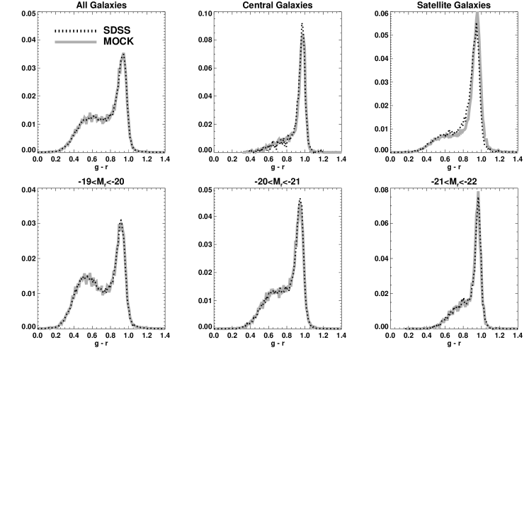
By repeating the above procedure in each luminosity bin, the color distribution of the mock galaxies is in exact agreement with the data, as can be seen in the top left and bottom panels of Figure 1. Note that this desirable property of our mock would be true regardless of the rank-ordering on The effect of the rank-ordering is to introduce, at fixed luminosity, a correlation between galaxy color and the epoch of starvation.
The property is based on three characteristic epochs of a halo’s mass assembly history. These include:
-
1.
The first epoch at which halo mass exceeds For halos that never attain this mass
-
2.
For subhalos, is the epoch after which the object always remains a subhalo. For host halos,
-
3
Using the methods of Wechsler et al. (2002) we identify the redshift at which the halo transitions from the fast- to slow-accretion regime, as this is the epoch after which dark matter ceases to accrete onto the halo’s central region.
From these three characteristic epochs we define the redshift of starvation:
| (2) |
We provide a full discussion of the physical motivation and interpretation of in § 6.3. In Appendix A, we discuss the details of how each of the above properties are computed from Bolshoi merger trees.
4.1.3 Algorithm Summary
For convenience, we conclude discussion of our mock-making algorithm by briefly summarizing the steps discussed above:
-
1.
From the Bolshoi halo catalog and merger trees, we compute and for every (sub)halo in the simulation.
-
2.
We assign r-band luminosities to the (sub)halos using abundance matching with the halo property Mock galaxies dimmer than are cut from the sample.
-
3.
The mock galaxies are binned by luminosity, and colors are assigned by randomly drawing from the color PDF defined by our SDSS Mr19 galaxy sample. The random draws from are rank-ordered, and the mock galaxies in each luminosity bin are rank-ordered by the halo property such that in each luminosity bin mock galaxies where occurs earlier are assigned redder colors.
4.2 Group Identification
Once colors and luminosities have been assigned to the halo catalog, we place our mock galaxies into redshift space and run the same group-finding algorithm on the mock that was run on the SDSS Mr19 galaxy sample. In this way, our mock groups inherit the same purity and incompleteness systematics as our SDSS groups. Finally, we introduce fiber collisions into our mock sample according to the prescription adopted in H12; this method preserves the relationship between local galaxy density and the likelihood that a fiber collision occurs in the SDSS Mr19 sample.
5 Results
We now investigate how well our model can predict a variety of observed galaxy statistics. First, we illustrate the general relationship between and and then demonstrate that our model naturally predicts the correct relative colors of central and satellite galaxies. We show the accuracy of our base Mr19 SDSS catalog at reproducing the observed SDSS luminosity-binned 2PCF, explicitly showing that our mock catalog naturally inherits the successes of abundance matching. We then compare the resulting color-binned 2PCF predictions to SDSS measurements. Finally, we test the success of our model against a variety of galaxy group statistics measured from the Mr19 group catalog.
5.1 Halo Age and Galaxy Color
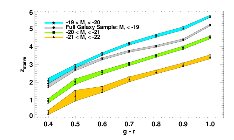
In Figure 2, we plot the mean value of (sub)halos in our mock in bins of color. The gray band shows the result for all mock galaxies in our sample, while the result in bins of luminosity appear in the colored bands. The width of the bands corresponds to bootstrap estimates of the error on the mean. This figure visually demonstrates the fundamental assumption of age distribution matching: redder galaxies tend to live in older halos. The luminosity dependence of the color relation simply reflects the color-luminosity trend seen in the data,
The values of may seem strikingly large. Indeed, the reddest galaxies in our model typically have This highlights an important point: the property does not correspond to the redshift where star formation in the galaxy is quenched. Rather, signifies a special epoch in halo assembly that correlates strongly with the epoch when star formation in the galaxy becomes inefficient. In our color assignment algorithm (described in § 4.1.2), rank-ordering on only serves to govern the relative colors assigned to halos; drawing the assigned colors from ensures that the absolute values of the assigned colors are correct. Thus in the (likely) event that there is a substantial time delay between and provided that this time delay does not strongly vary with halo mass then rank-ordering on should still suffice to assign the right colors to the right halos. We return to this point in § 6.
5.2 Central and Satellite Colors
As discussed in § 4.1.2, our model correctly reproduces the color distribution by construction. However, this by no means guarantees that our color PDF will be correctly predicted when conditioned on some other property besides luminosity. In the top center and top right panels of Figure 1, we show the color PDFs of our entire sample, conditioned on whether the galaxy is a central or satellite, respectively.
Our color assignment only uses the property and to assign colors to the mock galaxies but does not distinguish between centrals and satellites. Thus the good agreement seen between our model and the data in the top center and top right panels of Figure 1 demonstrates a successful prediction of age distribution matching. In our model, central and satellite galaxies have different color distributions because host halos and subhalos have different mass assembly histories.
5.3 Luminosity- and Color-Dependent Clustering
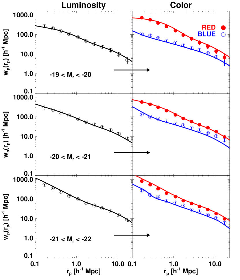
We begin discussion of our clustering results by showing that our abundance matching-based luminosity assignment (described in § 4.1.1) accurately predicts the observed luminosity-binned 2PCF as measured by Zehavi et al. (2011). To do this, we take our volume-limited Mr19 catalog and sub-divide into three luminosity bins: , , and . For each of these luminosity bins, we compute the real-space 2PCF. We then convert to projected space, , via:
| (3) |
For the upper limit in the integration, we use to be consistent with the measurements made for our observational samples.
The black solid curves in the left column of Figure 3 show the 2PCF as predicted by our mock catalog. There is excellent agreement with the Zehavi et al. (2011) SDSS measurements (black data points) at each luminosity bin and at all projected separations from the linear to highly non-linear regimes.
From this success, we now turn to the right column of Figure 3 showing the color-dependent 2PCFs in distinct -band luminosity bins as predicted by our age distribution matching formalism. Red filled and blue open circles in all panels represent the red and blue galaxy populations from Zehavi et al. (2011), respectively. Red and blue solid curves are the model predictions. While there is some discrepancy between the clustering of blue galaxies in the model and the data at large scales for the bin, overall there is good agreement for each luminosity bin and at all separation scales. This result is very encouraging since the color-dependent 2PCF encodes rich information about the galaxy-halo connection (e.g., More et al., 2013; Cacciato et al., 2013). However, as shown in Masaki et al. (2013) the 2PCF alone is not enough to discriminate between competing models for the relationship between a halo and the color of the galaxy it hosts (see also Neistein et al. (2011)). We address this in the next section with our exploration of galaxy group statistics.
We emphasize that we have done no parameter fitting to achieve the agreement between the predicted and measured color-binned clustering. Our algorithm for color assignment has no explicit dependence on halo position; rather, the clustering signal in our mock emerges as a prediction of our theory. Since the primary aim of this paper is to introduce the age distribution matching formalism, we have opted for the simplest implementation of this framework rather than attempting to finely tune our model according to the measured clustering (see § 6 for a discussion of more complex possible implementations). The success of our model’s prediction for the color-binned 2PCF is rather striking given the simplicity of the formulation we present here.
5.4 Galaxy Group Statistics
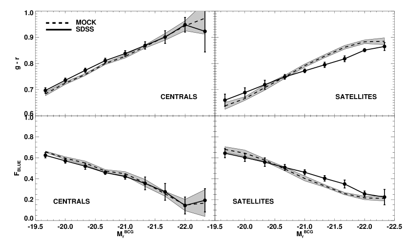
In this section we test how well our model distinctly assigns colors to satellite and central galaxies in our mock catalog compared to those colors in the SDSS galaxy group catalog. In the top row of Figure 4, we show the mean color of group galaxies as a function of the brightness of the group’s central galaxy, . From left to right, we show the results for central galaxies and satellites, respectively, in the mock and the SDSS group catalog. The dashed line traces the mean color of the mock galaxies in a given bin. The bottom row is similar to the top, except we plot the fraction of galaxies that are designated ‘blue’ according to the color cut defined by Eq. 1.
In all panels of Fig. 4, the solid gray region shows the errors on the mean. We use standard bootstrap resampling techniques to estimate the errors in all of our group-based statistics. We compute the errors as the dispersion over 1000 bootstrap realizations of the galaxy sample, where each realization is constructed by randomly selecting222We bootstrap resample with replacement, that is, we allow for the possibility of repeated draws of the same object. galaxies from the sample, where is the total number of galaxies in the sample.
The successful, distinct predictions for the colors of central and satellite galaxies emerges naturally from the age distribution matching formalism. At fixed luminosity, the colors of our mock galaxies are drawn from the same color PDF, regardless of sub/host halo designation. Moreover, our color assignment algorithm takes no explicit account of (sub)halo mass. Thus the difference between the colors of satellites and centrals in our mock is purely a reflection of the different mass assembly history of host halos and subhalos. Excepting only some mild tension for the color of satellite galaxies in a few of the brighter bins, the agreement between mock and observed central and satellite galaxy color is quite good. Again, we emphasize that we have not tuned any parameters in our model and we have chosen to keep our implementation of the age distribution matching technique as simple as possible (see § 6 for an elaboration of this point).
6 DISCUSSION & IMPLICATIONS
6.1 Comparison to Abundance Matching
Mock catalogs based on age distribution matching inherit all the successes of abundance matching because this is precisely the method we use in the luminosity assignment phase of our algorithm. The color PDF plays the same role in the color assignment that the luminosity function plays in the luminosity assignment. Thus just as from abundance matching agrees precisely with the observed luminosity function, so do our mock color distributions agree precisely with the observed color PDF.
There is an important conceptual difference between abundance matching and age distribution matching: the role that the property plays in the color assignment differs markedly from the role played by in the luminosity assignment. In abundance matching, luminosity assignment simply cannot proceed without appeal to the property (or some other halo property such as for host halos and for subhalos), because this is an essential ingredient to the defining relation This is not the case with the color assignment. While the dark matter halo property is in monotonic correspondence with color just as is in monotonic correspondence with luminosity, this feature is not essential in order for the color assignment algorithm to proceed. Indeed, the rank-ordering of color with only serves to correlate galaxy color with halo mass assembly history (at fixed ), but a mock catalog constructed without this correlation would nonetheless have a color PDF that is in agreement with
In light of this observation, one may wonder whether correlating galaxy color with is necessary at all in the construction of a successful model. However, a mock catalog constructed by drawing colors from the data without any rank-ordering predicts no difference between the clustering of red and blue samples (at fixed luminosity). This failure is easy to understand: in such a model colors are assigned purely at random, and so there is no mechanism which produces any trend between color and the cosmic density field.
6.2 Comparison to HOD models
In the standard implementation of the HOD formalism, the only halo property that governs galaxy occupation is the host halo mass, In particular, both Zehavi et al. (2011) and Skibba (2009) employ the HOD in their distinct approaches to modeling color-dependent clustering, and in neither model is there any explicit use of halo age. In the Zehavi et al. (2011) model, the HOD parameters of red and blue galaxy samples are constrained by two-point clustering together with galaxy abundance. In the alternative HOD approach explored in Skibba (2009), the authors draw colors for mock centrals and satellites from explicitly different distributions. Both models faithfully reproduce the color-dependence of the 2PCF (see also Skibba et al. (2013) for tests of color HOD models beyond binned 2PCF statistics).
The above HOD-based models assume that there are only two pieces of information that determine (in a statistical sense) the color of a galaxy: 1) whether the galaxy is a central or a satellite, and 2) the mass of the host halo in which the galaxy resides. As both of these models enjoy great success in reproducing observations, it may seem surprising that our model also succeeds since the color assignment phase of our algorithm appears to take no account of host halo mass. Moreover, in our model the only distinction between centrals and satellites is the use of yet for the majority () of subhalos at all luminosities. Thus our model also appears to assign colors to central and satellite galaxies in an identical fashion, at least in effect.
The resolution to this puzzle is illuminating. First, in CDM there is a strong correlation between halo mass and formation, with more massive halos forming at later times. Thus our model effectively does introduce rather strong trends between color and host halo mass due to the halo age-mass correlation. Thinking of as a proxy for host halo mass, these trends can readily be seen in Figure 4.
Second, at fixed mass, satellites and centrals have quite different assembly histories. This is true even when accounting for post-accretion stripping by comparing centrals to satellites at fixed mass at accretion, In general, at fixed satellites formed earlier than centrals, since satellites formed in denser regions of the initial density field and rapidly accreted their mass at earlier times. In age distribution matching, it therefore naturally emerges that satellites and centrals have different colors (Figure 1) even though we assign colors to them from the same PDF.
We conclude our discussion of models based only on host halo mass by noting that any model for galaxy color that depends strictly on is unable even in principle to reproduce the phenomenon of so-called Galactic Conformity: at fixed host mass, group systems with a blue central have a bluer satellite population than groups with a red central (Weinmann et al., 2006). This feature emerges naturally in the age distribution matching formalism, as we will demonstrate explicitly in a future companion paper.
6.3 Physical Motivation for
The expectation that should be related to stellar mass assembly is physically well-motivated. First, it is natural to expect that represents an important epoch in the history of the formation of a galaxy. As shown in Wechsler et al. (2002), at the dark matter halo transitions from the fast- to slow-accretion regime. After this epoch the matter accreting onto the dark matter halo ceases to penetrate into the core of the halo where the galaxy resides333See their Figure 18 for a demonstration of this point., depriving the galaxy of new material from the field with which it can form stars.
In reality, the halo may continue to form stars from its existing gas supply after this epoch, leading to a delay between and the actual quenching of star formation. However, our model is based on rank-ordering of the property and so the relative color of galaxies in halos with different formation times will be correct provided that this time delay is not a strong function of redshift or halo mass. As discussed in § 6.5, we will explore more complex models with quenching time delays in a future companion paper. We simply note here that corrections due to mass- and redshift-dependent time delays cannot be too severe or our model would not successfully predict the 2PCF and group-based statistics.
Second, the existence of a characteristic halo mass above which star formation is highly inefficient also has strong empirical support. The halo mass-dependence of the stellar mass to halo mass ratio of galaxies shows a peak at that rapidly falls off as halo mass increases (Yang et al., 2012, 2013; Watson & Conroy, 2013; Behroozi et al., 2012; Moster et al., 2013). This characteristic mass was recently shown to remain essentially constant for most of cosmic history (Behroozi et al., 2013). Additionally, is the halo mass at which pressure-supported shocks can heat infalling gas to the virial temperature (Dekel & Birnboim, 2006). More importantly, this is also the mass when effects due to AGN feedback become significant, which can have a dramatic effect on star formation (Shankar et al., 2006; Teyssier et al., 2011; Martizzi et al., 2012).
In our implementation of age distribution matching, we frame no hypothesis for the particular physical mechanism(s) that influence star formation inside massive halos. Instead, we simply posit that there exists a characteristic halo mass above which star formation becomes inefficient, and that this leads to a correlation between galaxy color and the characteristic epoch that the halo attains this mass.
We explored a range of masses for and find that both the 2PCF and our group statistics allow us to discriminate between competing values for the characteristic mass. In models where bright central galaxies are far too blue, and bright blue galaxies are strongly over-clustered on small scales (). Conversely, in models with central galaxies are too red and the 2PCF is in poor agreement with the data in all luminosity bins.
Finally, we turn to the property the epoch a satellite accreted onto its host halo. Numerous studies have shown that the dependence of galaxy color and/or star formation rate (SFR) has little-to-no residual environmental dependence once small-scale environment () has been accounted for (e.g., Hogg et al., 2004; Blanton et al., 2005). This small-scale environmental dependence has been shown to be driven primarily by correlations between the properties of the host halo and its satellite galaxies (Blanton & Berlind, 2007; Wetzel et al., 2011; Tinker et al., 2011; Wetzel et al., 2012). These results have given rise to a widely accepted picture in which satellite evolution is significantly influenced by processes that occur near or within the virial radius of the host halo.
There are a variety of physical mechanisms that may have a significant impact on satellite galaxy color/SFR. These include, but are not limited to, mass loss due to outside-in stripping (see Watson et al., 2012, and references therein), “strangulation” (Larson et al., 1980; Diemand et al., 2007; Kawata & Mulchaey, 2008), ram-pressure stripping (Gunn & Gott, 1972; Abadi et al., 1999; McCarthy et al., 2008), “harassment” (Moore et al., 1998), and intra-host mergers (Makino & Hut, 1997; Wetzel et al., 2009a, b). Again, in our implementation of age distribution matching, we do not preferentially select any one of these physical mechanisms as the primary cause for satellite quenching. Instead, we make the following simple observation: the impact that each of the scenarios discussed above has on satellite color/SFR will be greater for satellites that fell into their host halo potential at earlier times. Thus it is natural to expect a correlation between satellite galaxy color and . Accordingly, we identify as the third ’special’ epoch in (sub)halo mass accretion history.
Our treatment of the effect satellite accretion has on color/SFR is consistent with the finding in Wetzel et al. (2011) that there is no minimum host halo mass for post-accretion physics to significantly influence satellite evolution. Moreover, since we correlate color with regardless of host halo mass, the success of our implementation of age distribution matching provides new supporting evidence for conclusions drawn in van den Bosch et al. (2008), who found that satellite-specific processes are equally efficient in host halos of all masses.
With the above physical picture in mind, in age distribution matching we make the following simple assumption: the earlier any one of the above processes begins in a halo, the redder its galaxy will be today. Mathematically, this is formulated by introducing a monotonic correspondence between color and as described in § 4.1.2.
In alternative models that neglect to account for and instead define the clustering prediction for bright galaxies is in very poor agreement with the data. It is natural to expect that this failure would occur at the bright end: in such a model, group/cluster BCGs are all bright blue! This is because the halos hosting these BCGs are very massive and therefore very late-forming, and so without these halos have the smallest values of in the halo catalog. Conversely, models that neglect to account perform well at the bright end but fail to correctly predict the clustering of dimmer galaxies. Thus both and are essential ingredients to the success of age distribution matching.
The same is not true for models which do not account for subhalo accretion make quite similar predictions to those that do. This is because subhalos are typically not very massive objects that form very early on, and so for the typical subhalo This result may seem surprising since so much of the literature on star formation focuses squarely on the influence of satellite-specific quenching. Thus the success of our current model suggests that too much importance may have been placed on post-accretion physics (see also Watson & Conroy, 2013, for an alternative manifestation of this point). However, since there is likely a long time delay between and the actual quenching of star formation, we anticipate that subhalo accretion will prove to be more important when we more thoroughly explore models based on We return to this point in § 6.5.
6.4 Comparison to other phenomenological models
In a recent paper closely related to this work, Masaki et al. (2013) paint a binary ‘red’ or ‘blue’ color onto (sub)halos that have first been assigned luminosities based on abundance matching. The authors explored a variety of different halo properties to use in the color assignment. They found that several different choices result in successful predictions for the 2PCF, motivating their use of galaxy-galaxy lensing measurements to discriminate between competing models. Since precision galaxy-galaxy lensing measurements that have been binned simultaneously on both r-band luminosity and color were not available, the authors instead used measurements binned on morphology and assumed a perfect correspondence between red (blue) galaxies and early (late) type morphological classification.
While the assumption that all red (blue) galaxies have early (late) type morphology is a reasonable first approximation (Sheldon et al., 2004), we do not rely on it in this work. Instead, we employed galaxy group-based statistics to provide our additional discriminating power. Galaxy group membership yields information about halo occupation that is independent from 2PCF information. Group membership is necessarily identified in redshift space, and so group-based statistics incorporate information based on the velocity field, whereas projected clustering does not. Additionally, group statistics can probe halo occupation at higher masses than it is possible to do with small-scale clustering (see Hearin et al., 2012, Figure 2). Nonetheless, in a future companion paper to this one, we will make new galaxy-galaxy lensing measurements of SDSS galaxies binned on color to provide further tests of the success of the model we present here.
The semi-analytic modeling (SAM) approach to predicting galaxy properties such as color and star formation differs markedly from the theory presented here. SAMs also use the hierarchical build-up of dark matter halos as a foundation, but from here SAMs model the myriad baryonic processes that take place inside halos with a set of analytic formulae together with a large number of finely tuned parameters (White & Frenk, 1991; Kauffmann et al., 1999; Cole et al., 1994; Somerville & Primack, 1999; De Lucia & Blaizot, 2007; Guo et al., 2011). Such approaches have been quite successful at reproducing many statistics of the observed galaxy distribution, though the color-binned 2PCF has been notoriously difficult to correctly predict in quantitative detail (see, e.g., figures 20 & 21 of Guo et al., 2011).
There have been several recent advances in the literature on predicting galaxy color/SFR that dramatically simplify the set of assumptions and number of parameters required by most semi-analytic models. Mutch et al. (2013) couple dark matter halo accretion histories from the Millennium Simulation (Springel et al., 2005) with two simple analytic functions designed to encode the physics of baryonic growth and star formation history inside halos (see also Cattaneo et al., 2011, for a closely related formulation). Wang et al. (2007) also use halo accretion histories in the Millennium Simulation together with a model of stellar population synthesis to paint galaxies with spectral energy distributions and star formation rates onto dark matter halos; after fitting for two quenching time parameters, their model enjoys similar success to ours at predicting two-point clustering statistics. Peng et al. (2010); Peng et al. (2012) begins with a minimal set of phenomenological observations based on zCOSMOS data (Lilly et al., 2007) and apply a set of continuity equations to the evolution of the number of red and blue galaxies in order to connect galaxy properties to the dark matter halos hosting them (see also Lilly et al., 2013). The “separability condition” discussed in Peng et al. (2010) is reflected by our formulation of the property in that and are calculated purely independently for each halo.
The studies discussed above, (that is, Mutch et al., 2013; Lilly et al., 2013; Peng et al., 2012) assume a small set of simple analytic formulae together with knowledge of structure formation in to accurately reproduce a wide variety of one-point statistics of the galaxy distribution. By contrast, age distribution matching uses one-point statistics as input444Specifically the luminosity function and the distribution of colors . and correctly reproduces the two-point function (Figure 3) as well as higher-order statistics based on galaxy groups (Figure 4). The key to the success of our theory is the identification of a special time in each halo’s assembly history that is physically associated with the slowing and ultimate quenching of star formation in the galaxy at the center of the halo.
6.5 Future Work
The primary aim of this paper is to introduce a new theoretical framework for studying the galaxy-halo connection, and to show that this model is successful even with our relatively simple implementation. Accordingly, wherever possible we have opted to employ simplifying approximations that are widely used in the literature rather than tuning our exploration of halo mass accretion history to provide better fits to the observations. For example, as discussed in Appendix A we assume that the formation history of dark matter halos can be encompassed by a single parameter, and we appeal to the results in Wechsler et al. (2002) in our use of halo concentration as a proxy for In this section we call direct attention to some of these simplifying assumptions, and discuss possible extensions of our model that we intend to explore in future work.
6.5.1 Consideration of Time Delays
As discussed at length in Wetzel et al. (2011), the robust bimodality of the specific star formation rate (SSFR) distribution at low-redshift constitutes compelling evidence that post-accretion quenching of satellite star formation occurs rapidly after substantial time delay (Gyr). This motivates a modification to the formalism we introduce here, in which rather than the color of environment-quenched satellites is instead correlated with We have conducted a preliminary investigation of such models, finding that Gyr has little effect on either the 2PCF or the group statistics. However, the physical processes leading to a correlation between color and may also have a delayed onset, for example due to the length of time required for a pressure-supported shock to propagate to the virial radius. Since the physics underlying these two delays ( and ) is likely quite distinct, there is no reason to assume that they are equal. We postpone a more systematic investigation of this parameter space for the companion paper mentioned above.
6.5.2 Implementation of Scatter
In abundance matching, there is scatter between luminosity and In this work, we have assumed a purely monotonic relation between color and the property but it is easy to imagine implementations of age distribution matching in which there is scatter in this relation as well. A simple way to accomplish this would be an adaptation of the scatter method detailed in Appendix A of Hearin et al. (2012). Briefly, one would simply introduce Gaussian noise in the randomly drawn colors and use the rankings of the noisy values to appropriately shuffle the ranking of the (sub)halos. Again, we have not pursued this complication because our present aim is to show that even the simplest formulation of age distribution matching is remarkably successful. However, we intend to explore such extensions in future investigations of this technique, particularly when color-binned galaxy-galaxy lensing measurements become available.
6.5.3 Generalizations of the Model
In this paper, we have only investigated our theory at low redshift. However, if the luminosity function and color PDF are well measured at other epochs then our model should be consistent across redshifts, and this is a crucial next step for testing the generality of our age distribution matching formalism. Furthermore, our formalism generalizes in the obvious way to mock galaxies with stellar mass and/or (S)SFR instead of luminosity. We intend to study mocks based on such properties in the future as these are fundamental galaxy properties and are more directly linked to color (for example, due to dust attenuation). Such tests will be enabled by existing 2PCF measurements as a function of stellar mass split on blue and red galaxy populations at (Li et al., 2006; Jiang et al., 2011) and also (Mostek et al., 2012).
Our model is also general in the sense that the first phase of the algorithm need not necessarily be abundance matching. For example, one could instead begin by using the CLF formalism to assign brightnesses to dark matter halos. Alternatively, a stellar mass to halo mass map could be applied to construct a mock based on stellar masses. In either case, the color assignment phase of the algorithm would proceed in an identical fashion to what is described in § 4.1.2.
Finally, we note that in this work we have not explicitly illustrated the relationships between halo mass, and luminosity (stellar mass), nor have we presented the relative importance of and as a function of halo mass and luminosity (stellar mass). Such an investigation is of direct physical interest and may yield important insights into galaxy formation and evolution. We intend to conduct a detailed study of these relationships in future work once we have thoroughly explored more complex implementations of the age distribution matching technique along with the inclusion of additional observational constraints..
7 SUMMARY
In this section we summarize our primary results and conclusions:
-
1.
We introduce age distribution matching, a new theoretical framework for studying the relationship between halo mass accretion history and stellar mass assembly.
-
2.
By construction, over the entire luminosity range of our sample the color PDF of mock galaxies based on age distribution matching is in exact agreement with
-
3.
Our model successfully predicts luminosity- and color-binned two-point projected galaxy clustering at low-redshift, as well as central and satellite galaxy color as a function of host halo environment (). We emphasize that these are predictions of the theory, and that we have not relied upon any fitting or fine-tuning of any model parameters.
-
4.
The success of our model implies that the assembly history of galaxies and halos are indeed correlated.
-
5.
We make publicly available
-
•
Our mock galaxy catalog.
-
•
Full mass accretion histories of the main progenitors of all Bolshoi halos.
-
•
8 acknowledgments
APH and DFW are particularly grateful to Andrey Kravtsov for invaluable feedback throughout the development of this work. We also thank Matt Becker, Benedikt Diemer, Simon Lilly, Jeff Newman, Andrew Zentner, Idit Zehavi, Jennifer Piscionere, and Nick Gnedin for useful discussions at various stages, and Charlie Conroy and Frank van den Bosch for comments on an early draft. We thank Andreas Berlind for the use of his group finder and for early discussions about this type of modeling, and Peter Behroozi for making his halo catalogs and merger trees publicly available, and also for reliably prompt and clear answers to questions about these catalogs. We thank Ramin Skibba for sharing his mock catalog with us and for many informative discussions. We are grateful to an anonymous referee for valuable contributions to our first draft. Finally, we thank John Fahey for Transfigurations of Blind Joe Death.
APH is also supported by the U.S. Department of Energy under contract No. DE-AC02-07CH11359. DFW is supported by the National Science Foundation under Award No. AST-1202698.
References
- Abadi et al. (1999) Abadi M. G., Moore B., Bower R. G., 1999, MNRAS , 308, 947
- Abazajian et al. (2009) Abazajian K. N., Adelman-McCarthy J. K., Agüeros M. A., Allam S. S., Allende Prieto C., An D., Anderson K. S. J., Anderson S. F., Annis J., Bahcall N. A., et al. 2009, ApJS , 182, 543
- Baldry et al. (2004) Baldry I. K., Glazebrook K., Brinkmann J., Ivezić Ž., Lupton R. H., Nichol R. C., Szalay A. S., 2004, ApJ , 600, 681
- Balogh et al. (1999) Balogh M. L., Morris S. L., Yee H. K. C., Carlberg R. G., Ellingson E., 1999, ApJ , 527, 54
- Behroozi et al. (2010) Behroozi P. S., Conroy C., Wechsler R. H., 2010, ApJ , 717, 379
- Behroozi et al. (2013a) Behroozi P. S., et al., 2013a, ApJ , 763, 18
- Behroozi et al. (2013b) Behroozi P. S., et al., 2013b, ApJ , 762, 109
- Behroozi et al. (2012) Behroozi P. S., Wechsler R. H., Conroy C., 2012, ArXiv:1207.6105
- Behroozi et al. (2013) Behroozi P. S., Wechsler R. H., Conroy C., 2013, ApJL , 762, L31
- Bell et al. (2004) Bell E. F., et al., 2004, ApJ , 608, 752
- Berlind et al. (2006) Berlind A. A., et al., 2006, ApJS , 167, 1
- Berlind & Weinberg (2002) Berlind A. A., Weinberg D. H., 2002, ApJ , 575, 587
- Blanton & Berlind (2007) Blanton M. R., Berlind A. A., 2007, ApJ , 664, 791
- Blanton et al. (2005) Blanton M. R., Eisenstein D., Hogg D. W., Schlegel D. J., Brinkmann J., 2005, ApJ , 629, 143
- Blanton et al. (2003) Blanton M. R., et al., 2003, ApJ , 594, 186
- Blumenthal et al. (1984) Blumenthal G. R., Faber S. M., Primack J. R., Rees M. J., 1984, Nature , 311, 517
- Bryan & Norman (1998) Bryan G. L., Norman M. L., 1998, ApJ , 495, 80
- Cacciato et al. (2013) Cacciato M., van den Bosch F. C., More S., Mo H., Yang X., 2013, MNRAS , 430, 767
- Carollo et al. (2012) Carollo C. M., et al., 2012, ArXiv:1206.5807
- Cattaneo et al. (2011) Cattaneo A., Mamon G. A., Warnick K., Knebe A., 2011, AAP, 533, A5
- Cole et al. (1994) Cole S., Aragon-Salamanca A., Frenk C. S., Navarro J. F., Zepf S. E., 1994, MNRAS , 271, 781
- Conroy & Wechsler (2009) Conroy C., Wechsler R. H., 2009, ApJ , 696, 620
- Conroy et al. (2006) Conroy C., Wechsler R. H., Kravtsov A. V., 2006, ApJ , 647, 201
- Cooper et al. (2006) Cooper M. C., et al., 2006, MNRAS , 370, 198
- Cooper et al. (2012) Cooper M. C., et al., 2012, MNRAS , 419, 3018
- Cooray & Sheth (2002) Cooray A., Sheth R., 2002, Phys. Rep. , 372, 1
- De Lucia & Blaizot (2007) De Lucia G., Blaizot J., 2007, MNRAS , 375, 2
- Dekel & Birnboim (2006) Dekel A., Birnboim Y., 2006, MNRAS , 368, 2
- Diemand et al. (2007) Diemand J., Kuhlen M., Madau P., 2007, ApJ , 667, 859
- Gerke et al. (2012) Gerke B. F., Wechsler R. H., Behroozi P. S., Cooper M. C., Yan R., Coil A. L., 2012, ArXiv:1207.2214
- Gottloeber & Klypin (2008) Gottloeber S., Klypin A., 2008, ArXiv:0803.4343
- Gunn & Gott (1972) Gunn J. E., Gott III J. R., 1972, ApJ , 176, 1
- Guo et al. (2012) Guo H., Zehavi I., Zheng Z., 2012, ApJ , 756, 127
- Guo et al. (2011) Guo Q., White S., Boylan-Kolchin M., De Lucia G., Kauffmann G., Lemson G., Li C., Springel V., Weinmann S., 2011, MNRAS , 413, 101
- Guo et al. (2010) Guo Q., White S., Li C., Boylan-Kolchin M., 2010, MNRAS , 404, 1111
- Hearin et al. (2012) Hearin A. P., Zentner A. R., Berlind A. A., Newman J. A., 2012, ArXiv:1210.4927
- Hearin et al. (2012) Hearin A. P., Zentner A. R., Newman J. A., Berlind A. A., 2012, ArXiv:1207.1074
- Hogg et al. (2004) Hogg D. W., et al., 2004, ApJL , 601, L29
- Jiang et al. (2011) Jiang T., Hogg D. W., Blanton M. R., 2011, ArXiv:1104.5483
- Kauffmann et al. (1999) Kauffmann G., Colberg J. M., Diaferio A., White S. D. M., 1999, MNRAS , 303, 188
- Kawata & Mulchaey (2008) Kawata D., Mulchaey J. S., 2008, ApJL , 672, L103
- Klypin et al. (2011) Klypin A. A., Trujillo-Gomez S., Primack J., 2011, ApJ , 740, 102
- Krause et al. (2013) Krause E., Hirata C. M., Martin C., Neill J. D., Wyder T. K., 2013, MNRAS , 428, 2548
- Kravtsov (2013) Kravtsov A. V., 2013, ApJL , 764, L31
- Kravtsov et al. (2004) Kravtsov A. V., Berlind A. A., Wechsler R. H., Klypin A. A., Gottlöber S., Allgood B., Primack J. R., 2004, ApJ , 609, 35
- Kravtsov et al. (1997) Kravtsov A. V., Klypin A. A., Khokhlov A. M., 1997, ApJS , 111, 73
- Larson et al. (1980) Larson R. B., Tinsley B. M., Caldwell C. N., 1980, ApJ , 237, 692
- Leauthaud et al. (2011) Leauthaud A., et al., 2011, ArXiv:1104.0928
- Li et al. (2006) Li C., Kauffmann G., Jing Y. P., White S. D. M., Börner G., Cheng F. Z., 2006, MNRAS , 368, 21
- Lilly et al. (2013) Lilly S. J., Carollo C. M., Pipino A., Renzini A., Peng Y., 2013, ArXiv:1303.5059
- Lilly et al. (2007) Lilly S. J., et al., 2007, ApJS , 172, 70
- Makino & Hut (1997) Makino J., Hut P., 1997, ApJ , 481, 83
- Martizzi et al. (2012) Martizzi D., Teyssier R., Moore B., 2012, MNRAS , 420, 2859
- Masaki et al. (2013) Masaki S., Lin Y.-T., Yoshida N., 2013, ArXiv e-prints
- McCarthy et al. (2008) McCarthy I. G., Frenk C. S., Font A. S., Lacey C. G., Bower R. G., Mitchell N. L., Balogh M. L., Theuns T., 2008, MNRAS , 383, 593
- Moore et al. (1998) Moore B., Lake G., Katz N., 1998, ApJ , 495, 139
- More et al. (2009) More S., van den Bosch F. C., Cacciato M., Mo H. J., Yang X., Li R., 2009, MNRAS , 392, 801
- More et al. (2013) More S., van den Bosch F. C., Cacciato M., More A., Mo H., Yang X., 2013, MNRAS , 430, 747
- More et al. (2011) More S., van den Bosch F. C., Cacciato M., Skibba R., Mo H. J., Yang X., 2011, MNRAS, 410, 210
- Mostek et al. (2012) Mostek N., Coil A. L., Cooper M. C., Davis M., Newman J. A., Weiner B., 2012, ArXiv:1210.6694
- Moster et al. (2013) Moster B. P., Naab T., White S. D. M., 2013, MNRAS , 428, 3121
- Moster et al. (2010) Moster B. P., Somerville R. S., Maulbetsch C., van den Bosch F. C., Macciò A. V., Naab T., Oser L., 2010, ApJ , 710, 903
- Mutch et al. (2013) Mutch S. J., Croton D. J., Poole G. B., 2013, ArXiv:1304.2774
- Neistein et al. (2011) Neistein E., Li C., Khochfar S., Weinmann S. M., Shankar F., Boylan-Kolchin M., 2011, MNRAS, 416, 1486
- Neistein et al. (2010) Neistein E., Weinmann S. M., Li C., Boylan-Kolchin M., 2010, ArXiv:1011.2492
- Norberg et al. (2002) Norberg P., et al., 2002, MNRAS , 332, 827
- Peacock & Smith (2000) Peacock J. A., Smith R. E., 2000, MNRAS , 318, 1144
- Peng et al. (2010) Peng Y.-j., et al., 2010, ApJ , 721, 193
- Peng et al. (2012) Peng Y.-j., Lilly S. J., Renzini A., Carollo M., 2012, ApJ , 757, 4
- Pizagno et al. (2007) Pizagno J., et al., 2007, AJ , 134, 945
- Reddick et al. (2012) Reddick R. M., Wechsler R. H., Tinker J. L., Behroozi P. S., 2012, ArXiv:1207.2160
- Riebe et al. (2011) Riebe K., Partl A. M., Enke H., Forero-Romero J., Gottloeber S., Klypin A., Lemson G., Prada F., Primack J. R., Steinmetz M., Turchaninov V., 2011, ArXiv:1109.0003
- Rodríguez-Puebla et al. (2012) Rodríguez-Puebla A., Drory N., Avila-Reese V., 2012, ApJ , 756, 2
- Scoccimarro et al. (2001) Scoccimarro R., Sheth R. K., Hui L., Jain B., 2001, ApJ , 546, 20
- Seljak (2000) Seljak U., 2000, MNRAS , 318, 203
- Shankar et al. (2006) Shankar F., Lapi A., Salucci P., De Zotti G., Danese L., 2006, ApJ , 643, 14
- Sheldon et al. (2004) Sheldon E. S., Johnston D. E., Frieman J. A., Scranton R., McKay T. A., Connolly A. J., Budavári T., Zehavi I., Bahcall N. A., Brinkmann J., Fukugita M., 2004, AJ , 127, 2544
- Simha et al. (2010) Simha V., Weinberg D., Dave R., Fardal M., Katz N., Oppenheimer B. D., 2010, ArXiv:1011.4964
- Skibba (2009) Skibba R. A., 2009, MNRAS , 392, 1467
- Skibba & Sheth (2009) Skibba R. A., Sheth R. K., 2009, MNRAS , 392, 1080
- Skibba et al. (2013) Skibba R. A., Sheth R. K., Croton D. J., Muldrew S. I., Abbas U., Pearce F. R., Shattow G. M., 2013, MNRAS, 429, 458
- Skibba et al. (2007) Skibba R. A., Sheth R. K., Martino M. C., 2007, MNRAS , 382, 1940
- Skibba et al. (2011) Skibba R. A., van den Bosch F. C., Yang X., More S., Mo H., Fontanot F., 2011, MNRAS, 410, 417
- Somerville & Primack (1999) Somerville R. S., Primack J. R., 1999, MNRAS , 310, 1087
- Springel et al. (2005) Springel V., White S. D. M., Jenkins A., Frenk C. S., Yoshida N., Gao L., Navarro J., Thacker R., Croton D., Helly J., Peacock J. A., Cole S., Thomas P., Couchman H., Evrard A., Colberg J., Pearce F., 2005, Nature , 435, 629
- Tasitsiomi et al. (2004) Tasitsiomi A., Kravtsov A. V., Wechsler R. H., Primack J. R., 2004, ApJ , 614, 533
- Teyssier et al. (2011) Teyssier R., Moore B., Martizzi D., Dubois Y., Mayer L., 2011, MNRAS , 414, 195
- Tinker et al. (2011) Tinker J., Wetzel A., Conroy C., 2011, ArXiv:1107.5046
- Tinker & Wetzel (2010) Tinker J. L., Wetzel A. R., 2010, ApJ , 719, 88
- Vale & Ostriker (2004) Vale A., Ostriker J. P., 2004, MNRAS , 353, 189
- Vale & Ostriker (2006) Vale A., Ostriker J. P., 2006, MNRAS , 371, 1173
- van den Bosch et al. (2008) van den Bosch F. C., Aquino D., Yang X., Mo H. J., Pasquali A., McIntosh D. H., Weinmann S. M., Kang X., 2008, MNRAS , 387, 79
- van den Bosch et al. (2007) van den Bosch F. C., Yang X., Mo H. J., Weinmann S. M., Macciò A. V., More S., Cacciato M., Skibba R., Kang X., 2007, MNRAS , 376, 841
- Wang et al. (2007) Wang L., Li C., Kauffmann G., De Lucia G., 2007, MNRAS , 377, 1419
- Watson et al. (2012) Watson D. F., Berlind A. A., McBride C. K., Hogg D. W., Jiang T., 2012, ApJ , 749, 83
- Watson et al. (2012) Watson D. F., Berlind A. A., Zentner A. R., 2012, ApJ , 754, 90
- Watson & Conroy (2013) Watson D. F., Conroy C., 2013, ArXiv:1301.4497
- Wechsler et al. (2002) Wechsler R. H., Bullock J. S., Primack J. R., Kravtsov A. V., Dekel A., 2002, ApJ , 568, 52
- Weinmann et al. (2009) Weinmann S. M., Kauffmann G., van den Bosch F. C., Pasquali A., McIntosh D. H., Mo H., Yang X., Guo Y., 2009, MNRAS , 394, 1213
- Weinmann et al. (2006) Weinmann S. M., van den Bosch F. C., Yang X., Mo H. J., 2006, MNRAS , 366, 2
- Wetzel et al. (2009a) Wetzel A. R., Cohn J. D., White M., 2009a, MNRAS , 395, 1376
- Wetzel et al. (2009b) Wetzel A. R., Cohn J. D., White M., 2009b, MNRAS , 394, 2182
- Wetzel et al. (2011) Wetzel A. R., Tinker J. L., Conroy C., 2011, ArXiv:1107.5311
- Wetzel et al. (2012) Wetzel A. R., Tinker J. L., Conroy C., van den Bosch F. C., 2012, ArXiv:1206.3571
- Wetzel et al. (2013) Wetzel A. R., Tinker J. L., Conroy C., van den Bosch F. C., 2013, ArXiv:1303.7231
- Wetzel & White (2010) Wetzel A. R., White M., 2010, MNRAS , 403, 1072
- Whitaker et al. (2011) Whitaker K. E., et al., 2011, ApJ , 735, 86
- White & Frenk (1991) White S. D. M., Frenk C. S., 1991, ApJ , 379, 52
- White & Rees (1978) White S. D. M., Rees M. J., 1978, MNRAS , 183, 341
- Wyder et al. (2007) Wyder T. K., et al., 2007, ApJS, 173, 293
- Yang et al. (2003) Yang X., Mo H. J., van den Bosch F. C., 2003, MNRAS , 339, 1057
- Yang et al. (2013) Yang X., Mo H. J., van den Bosch F. C., Bonaca A., Li S., Lu Y., Lu Y., Lu Z., 2013, ArXiv:1302.1265
- Yang et al. (2011) Yang X., Mo H. J., van den Bosch F. C., Zhang Y., Han J., 2011, ArXiv:1110.1420
- Yang et al. (2012) Yang X., Mo H. J., van den Bosch F. C., Zhang Y., Han J., 2012, ApJ , 752, 41
- York et al. (2000) York D. G., et al., 2000, AJ , 120, 1579
- Zehavi et al. (2002) Zehavi I., et al., 2002, ApJ , 571, 172
- Zehavi et al. (2005) Zehavi I., et al., 2005, ApJ , 630, 1
- Zehavi et al. (2011) Zehavi I., et al., 2011, ApJ , 736, 59
- Zheng et al. (2007) Zheng Z., Coil A. L., Zehavi I., 2007, ApJ , 667, 760
Appendix A
The central tenet of age distribution matching is that galaxy color is determined by halo mass accretion history, at least in a statistical sense. In this appendix we discuss the details of how we calculate and the key quantities used in the color assignment phase of our algorithm.
In accordance with the convention adopted in Behroozi et al. (2013a), we use the snapshot after which the subhalo always remains a subhalo. We also explored the definition of accretion advocated in Wetzel et al. (2013), where subhalos are said to have accreted the first time they have been identified as subhalos for two consecutive time-steps, and find that this choice has little impact on our results.
We use the approximation introduced in Wechsler et al. (2002), who find that mass accretion history is well-fit by an exponential, The authors in Wechsler et al. (2002) defined the scale factor of halo formation to be the epoch when the logarithmic slope of drops below While there is some amount of arbitrariness in this particular chosen value of the transition that occurs at or near this time has very real physical consequences: the central density of the halo ceases to increase (see their Figure 18). This physical change naturally gives rise to a correlation between halo formation time and NFW concentration (defined as the ratio of ).
One of the central results of Wechsler et al. (2002) is that is well-approximated by the following equation:
where and is the scale factor at the time of “observation”. For host halos we take the time of observation to be and use the halo’s concentration at this snapshot. Tidal disruption and mass stripping of subhalos after accretion makes estimates of noisy and unreliable. Fortunately, Wechsler et al. (2002) showed that the scaling of halo formation with remains the same over a broad range of So for subhalos, we define to be the NFW concentration of the subhalo at the time of accretion (as defined above). We note that for of subhalos, this definition produces an unphysically long tail at high redshift in the distribution. We attribute this to large, transient boosts to the subhalo concentration at due to a tidal event. However, we find that our results are insensitive to this behavior: when we collapse all objects in this tail to we get virtually identical results.
We use the first time a (sub)halo attains As noted in the main body of the paper, we explored a range of values of and found is the most successful.