The HETDEX Pilot Survey. IV. The Evolution of [O II] Emitting Galaxies from $z\sim 0.5$ to $z\sim 0$

Abstract

We present an analysis of the luminosities and equivalent widths of the 284 $z<0.56$ [O II]-emitting galaxies found in the 169 arcmin² pilot survey for the Hobby-Eberly Telescope Dark Energy Experiment (HETDEX). By combining emission-line fluxes obtained from the Mitchell spectrograph on the McDonald 2.7-m telescope with deep broadband photometry from archival data, we derive each galaxy’s de-reddened [O II] $\lambda 3727$ luminosity and calculate its total star formation rate. We show that over the last $\sim 5$ Gyr of cosmic time there has been substantial evolution in the [O II] emission-line luminosity function, with $L^{*}$ decreasing by $\sim 0.6\pm 0.2$ dex in the observed function, and by $\sim 0.9\pm 0.2$ dex in the de-reddened relation. Accompanying this decline is a significant shift in the distribution of [O II] equivalent widths, with the fraction of high equivalent-width emitters declining dramatically with time. Overall, the data imply that the relative intensity of star formation within galaxies has decreased over the past $\sim 5$ Gyr, and that the star formation rate density of the universe has declined by a factor of $\sim 2.5$ between $z\sim 0.5$ and $z\sim 0$. These observations represent the first [O II]-based star formation rate density measurements in this redshift range, and foreshadow the advancements which will be generated by the main HETDEX survey.

1. Introduction

The evolution in the cosmic star formation rate density (SFRD) is an important observational constraint for all the current models of galaxy formation and evolution (e.g., Somerville et al., 2012). It is generally agreed that the SFRD reached its peak around $z\sim 2$, and since then has declined by roughly an order of magnitude (e.g., Madau et al., 1996; Lilly et al., 1996; Hopkins & Beacom, 2006; Bouwens et al., 2010). However, the details of this evolution remain poorly understood, in part because of the systematic uncertainties associated with the patchwork of various star formation rate (SFR) indicators.

For example, in the nearby universe, the strength of the H$\alpha$ emission line is one of the most direct and robust measures of ongoing star formation, since it is powered by the photoionization produced by massive ($M\gtrsim 10M_{\odot}$), young ($t\lesssim 20$ Myr) stars (Kennicutt, 1998). Unfortunately, at distances greater than $z\sim 0.4$, this line redshifts out of the optical and into the near-IR portion of the spectrum, where it is much more difficult to observe (e.g., Glazebrook et al., 2004). Consequently, by $z\sim 1$, the [O II] $\lambda 3727$ emission line, which is produced by collisional excitation, has taken the place of H$\alpha$ (e.g., Hippelein et al., 2003; Ly et al., 2007), and by $z\gtrsim 2$, the preferred indicator of star formation is the rest-frame ultraviolet continuum (e.g., Pettini et al., 2001; Hopkins, 2004). Like the emission-line indicators, the rest-frame UV directly traces the flux of young, massive stars, but in this case, the timescale over which the star formation is measured is $\sim 100$ Myr, and the result is much more sensitive to internal extinction. Mid-IR measurements, which reflect the re-radiation of stellar emission by warm dust, integrate star formation over an even longer ($\sim 1$ Gyr) timescale (Kelson & Holden, 2010), further complicating the interpretation of the low-$z$ epoch, when the SFRD of the universe is evolving rapidly.

In practice, a large number of additional star formation rate indicators are used both at high and low redshift, and these span the entire electromagnetic spectrum, from 1.4 GHz radio and far-IR bands to the X-ray (see Hopkins, 2004, and references therein). One of the most versatile of these is the flux from the [O II] doublet at 3727 Å. As a SFR indicator, [O II] has two significant advantages over measurements in the near and far UV: it is easier to detect at low and intermediate ($z\lesssim 2$) redshifts and it is more sensitive to the instantaneous star formation rate, rather than the $\sim 100$ Myr time-averaged rate. Unfortunately, the path from [O II] emission to star formation rate is much less direct than for either H$\alpha$ or the near-UV, as the emission depends on parameters such as the galactic oxygen abundance and the ionization state of the gas (Kennicutt, 1998). Thus, the method must be calibrated empirically via comparisons to other SFR indicators (e.g., Jansen et al., 2001; Kewley et al., 2004; Moustakas et al., 2006).

Over the past 15 years, there have been several [O II]-based measurements of SFRDs, mostly at $z\sim 0$ and $z\sim 1$. Many of these studies derive from spectroscopic observations of magnitude-limited samples of galaxies, and are thus severely incomplete at the faint end of the emission-line luminosity function (Hogg et al., 1998; Hammer et al., 1997; Zhu et al., 2009). Others are based on narrow-band surveys of selected high redshift ($z>0.8$) epochs, and are thus only sensitive to high equivalent width objects (e.g., Ly et al., 2007; Takahashi et al., 2007). Still others employ near-IR Fabry-Perot observations and are restricted to the very brightest ($\sim 1$ dex) [O II] emitters at $z\sim 1$ (Hippelein et al., 2003). Consequently, while the local ($z<0.2$) [O II] luminosity function is reasonably well defined (Gallego et al., 1996; Gilbank et al., 2010), measurements of the evolution of [O II] $\lambda 3727$ emission over the last $\sim 5$ Gyr of cosmic time are rather limited. In fact, the only studies that attempt to sample the full-range [O II] over these intermediate redshifts are the Hubble Space Telescope grism surveys of Teplitz et al. (2003) and Pirzkal et al. (2012). Unfortunately, these $z\gtrsim 0.5$ observations are limited by a rather high equivalent width limit ($>35$ Å), and a lack of information concerning the galaxies’ internal extinction.

There is, however, one other dataset that can be exploited to measure the evolution of [O II] emission in the nearby universe. The pilot survey for the Hobby-Eberly Telescope Dark Energy Experiment (HETDEX) obtained blind integral field spectroscopy over 169 arcmin² of sky and measured [O II] $\lambda 3727$ fluxes for 284 galaxies between $0<z<0.56$ (Adams et al., 2011). Only a few [O II] surveys cover this redshift range, and most are defined by magnitude-limited samples of objects. In contrast, the HETDEX pilot survey’s dataset is emission-line flux limited, rather than continuum flux limited, and is thus complete to much lower star formation rates than surveys which choose their targets via broadband measurements. The observations therefore sample a section of parameter space rarely probed by other investigations, and is a unique resource for studying the relationship between [O II] and other star formation rate indicators. Moreover, because the HETDEX pilot survey was conducted in fields with large amounts of ancillary data, we also have access to each galaxy’s spectral energy distribution (SED), enabling a full examination of its photometric properties and internal reddening. Finally, because the survey’s redshift range covers the last $\sim 5$ Gyr of cosmic time, the database can be used to trace the late-time evolution of [O II], and provide a comparison for SFRD measurements obtained at higher redshift.

In this paper, we present an analysis of the [O II] $\lambda 3727$ emission-line galaxies found in the HETDEX pilot survey. In §2, we summarize the observations and the selection method which produced the catalog of 284 [O II] line emitters. In §3, we present the evolution of the [O II] equivalent width distribution with redshift, and use this reddening-independent quantity to show how the relative importance of star formation has declined over the last $\sim 5$ Gyr. In §4, we examine the internal extinction of the [O II] emitters, and compare the star formation rates derived from the measurements of the [O II] flux to those determined via the rest-frame UV continuum. In §5, we present both observed- and extinction-corrected [O II] luminosity functions and explore the evolution of the cosmic SFRD out to $z\sim 0.5$. We conclude by discussing the implications of our work for future surveys of star-forming galaxies.

Throughout this work, we adopt a $\Lambda$CDM cosmology with $\Omega_{m}=0.3$, $\Omega_{\Lambda}=0.7$ and $H_{0}=70$ km s^-1 Mpc^-1.

2. The HETDEX Pilot Survey Data

The data for our analysis were taken as part of the HETDEX pilot survey, a blind integral-field spectroscopic study of four areas of sky containing a wealth of ancillary multi-wavelength data: COSMOS (Scoville et al., 2007), GOODS-N (Giavalisco et al., 2004), MUNICS-S2 (Drory et al., 2001), and XMM-LSS (Pierre et al., 2004). A complete description of this pathfinding survey and its data products is given in Adams et al. (2011). Briefly, a square 246-fiber array was mounted on the Harlan J. Smith 2.7-m telescope at McDonald Observatory, and coupled to the George and Cynthia Mitchell Spectrograph, a proto-type of the Visible Integral-field Replicable Unit Spectrograph (VIRUS) designed for HETDEX (Hill et al., 2008b). This instrument was set to disperse the wavelength range between 3600 Å and 5800 Å at $\sim 5$ Å resolution and 1.1 Å pixel^-1. Each fiber subtended $4\farcs 2$ on the sky; consequently, the entire fiber array covered an area of $1\farcm 7\times 1\farcm 7$ with a 1/3 fill factor. To fill in the fiber gaps and improve the survey’s spatial resolution, each field was observed using a 6-pointing dither pattern, generating $6\times 246=1,476$ separate spectra. In total, the pilot survey covered 169 arcmin² of blank sky (71.6 arcmin² in COSMOS, 35.5 arcmin² in GOODS-N, 49.9 arcmin² in MUNICS-S2, and 12.3 arcmin² in XMM-LSS) with 1 hour of exposure time at each dither position. Fifty percent of the pointings reached a $5\,\sigma$ monochromatic flux limit of $6.7\times 10^{-17}$ ergs cm^-2 s^-1 at 5000 Å, and 90% reached $1.0\times 10^{-16}$ ergs cm^-2 s^-1. Simulations demonstrate that for objects with equivalent widths greater than $\sim 5$ Å, the recovery fraction of emission lines integrated across all continuum brightnesses is greater than 95%, and even for equivalent widths as small as 1 Å, the completeness fraction is better than 90%.

The goal of the HETDEX pilot survey was to test the equipment, analysis procedures, and ancillary data requirements for the main HETDEX survey (Hill et al., 2008a) by performing an unbiased search for emission-line objects over a wide range of redshifts. To do this, each sky-subtracted fiber spectrum was first flux-calibrated and then searched for the presence of emission lines. When a candidate emission feature was found, the COSMOS, GOODS-N, MUNICS-S2, and XMM-LSS imaging data were used to identify the line’s photometric counterpart. The combination of the spectroscopic line flux and the photometrically determined continuum flux density were then used to calculate the line’s equivalent width. The identity of the emission line and the object’s most-likely redshift were then determined using either 1) the presence of multiple emission lines in the spectrum, 2) the source’s photometric spectral-energy distribution (as determined from the multi-wavelength images), or 3) the emission-line’s rest-frame equivalent width. The latter criterion is particularly useful for discriminating Ly$\alpha$ from local [O II] $\lambda 3727$, as single-line sources with rest-frame equivalent widths greater than 20 Å are almost always Ly$\alpha$ emitters (Gronwall et al., 2007).

In total, the HETDEX pilot survey identified 397 emission-line sources, including 104 Ly$\alpha$ emitters (Blanc et al., 2011), and 284 [O II] emission line galaxies. The latter have redshifts between $0.078<z<0.563$, [O II] emission-line luminosities between $39.8<\log L<42.2$ (ergs cm^-2 s^-1), and [O II] rest-frame equivalent widths as great as 77 Å.

3. Star Formation versus Emission from AGN

Before examining the issue of star formation in our emission-line galaxies, we first must consider the effect that active galactic nuclei have on our [O II] fluxes. The pilot survey spectra do not have the wavelength coverage to employ traditional line-ratio diagnostics such as [N II]/H$\alpha$ or [O III]/H$\beta$ for AGN detection (e.g., Baldwin et al., 1981; Veilleux & Osterbrock, 1987; Kewley et al., 2001). However, because the fields chosen for study have been studied with the Chandra and XMM observatories, we can identify probable AGN contaminants via X-ray luminosity.

In Adams et al. (2011), X-ray counterparts were identified for 30 of the HETDEX pilot survey’s [O II] emitters. However, many of these objects are in the GOODS-N region, where the Chandra images are deep enough to detect the X-rays associated with normal star formation (e.g., Persic et al., 2004; Lehmer et al., 2010). If we exclude the [O II] emitters with luminosities fainter than $10^{40}$ ergs s^-1 in the 2 to 8 keV X-ray band, we are left with 10 probable AGN: 5 in GOODS-N (which has the deepest X-ray coverage), and 5 in the other three fields. This number, which represents $\sim 3\%$ of the sample, is slightly greater than the AGN contamination rate of 1 to 2% estimated by Zhu et al. (2009) in their analysis of the line-ratios and X-ray emission of $z\sim 1$ [O II] emitters in the DEEP2 survey. Since the X-ray luminosity limits used here are more than an order of magnitude fainter than those considered by Zhu et al. (2009), we judge this agreement to be acceptable.

Of course, just because an object emits X-rays, it does not necessarily follow that the system’s integrated [O II] emission is dominated by flux from the central engine. Ho (2005) has shown that the physical conditions in the narrow-line regions of AGN disfavor the creation of strong [O II]. Indeed, an examination of the X-ray bright objects in our survey demonstrates that these likely AGN are generally not amongst the brightest [O II] sources. Consequently, their existence does not substantially alter the observed [O II] luminosity function or equivalent width distribution, nor do they effect the main conclusions of this paper. We therefore exclude these AGN candidates from our analysis.

4. The Equivalent Width Distribution

One quick but very coarse way of examining the relative importance of star formation as a function of time is through the use of the distribution of [O II] $\lambda 3727$ rest-frame equivalent widths. The [O II] flux from a galaxy generally measures the amount of star formation in the very recent past, i.e., $t\lesssim 20$ Myr (Kennicutt, 1998). In contrast, the continuum underlying 3727 Å in large part reflects star formation over a much longer ($\sim 1$ Gyr) timescale (Gilbank et al., 2010). Thus, by forming the ratio of these two quantities, it is possible to examine the relative importance of the current burst of star formation in a manner that reduces the complications introduced by internal extinction.

In the local neighborhood, the distribution of [O II] $\lambda 3727$ rest-frame equivalent widths peaks near $\sim 5$ Å, and then rapidly decays, as would an exponential with a scale length of $w_{0}\lesssim 10$ Å (Blanton & Lin, 2000). Notably, this function has virtually no dependence on the brightness of the galaxy: the distribution of rest-frame [O II] equivalent widths for the $\sim 8500$ galaxies discovered in the Las Campanas Redshift Survey is almost independent of $R$-band luminosity (Blanton & Lin, 2000). Similarly, there is no evidence for a correlation between luminosity and equivalent width in an H$\alpha$ grism-survey of the local universe: if we divide the 191 galaxies of the Gallego et al. (1996) survey in half and perform an Anderson-Darling test (Scholz & Stephens, 1987), we find no statistical difference between the distributions of [O II] equivalent widths for the high- and low-line luminosity samples.

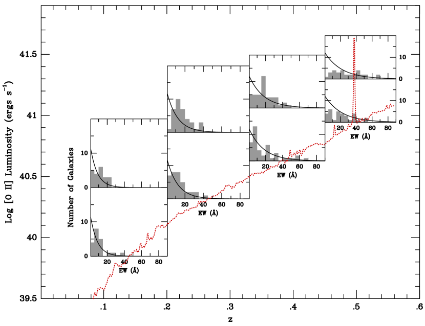
Figure 1.— The distribution of [O II] $\lambda 3727$ rest-frame equivalent widths for the pilot survey galaxies, plotted as a function of [O II] luminosity ($y$-axis) and redshift ($x$-axis). The location of each histogram illustrates the redshifts and (approximate) luminosities of the galaxies contained within it. The dotted red line shows the 80% detection limit, i.e., 80% of the survey frames have $5\sigma$ detection limits brighter than this threshold. The [O I] airglow feature at 5577 Å is easily seen. A total of 259 galaxies lie above the 80% threshold. The curves display how the best-fit exponential changes with redshift. Since the distribution of equivalent widths turns over at small values, objects with rest-frame equivalent widths less than 5 Å have been excluded from the calculation. The absence of high-luminosity [O II] emitters at low redshift is partially a volume effect. Note the distribution of equivalent widths is insensitive to [O II] luminosity, but is strongly dependent on redshift.

Figure 1 displays the rest-frame [O II] equivalent width distribution for the HETDEX pilot survey’s sample of emission-line galaxies, as a function of redshift and [O II] luminosity. Specifically, the figure sub-divides our sample of [O II] emitting galaxies into four redshift bins, and histograms the rest-frame equivalent widths for galaxies in the top-half and bottom-half of the emission-line luminosity function. The location of each histogram illustrates the redshifts and (approximate) luminosities of the galaxies contained within it. The dotted line in the figure illustrates the data’s “80% completeness limit,” i.e., 80% of the fields observed in the survey have $5\sigma$ detection limits brighter than this value. Only one out of the 42 galaxies at $z<0.2$ has a line-luminosity brighter than $\log L=41.1$; this is partially a volume effect, as the probability of finding a high-luminosity target in the nearby universe is small. Conversely, at $z>0.45$, low-luminosity [O II] emitters fall below the flux limit of the survey. Nevertheless, despite this selection effect, it is clear that any dependence of equivalent width on [O II] luminosity is minimal. While we cannot exclude the possibility of a small luminosity dependence in the equivalent width distribution, an Anderson-Darling test finds no significant difference between the high-luminosity and low-luminosity samples, even at the $1\sigma$ level.

Conversely, the redshift dependence of the rest-frame [O II] equivalent width distribution is quite strong, with the number of high-equivalent width objects increasing rapidly with redshift. At $z<0.2$, the median rest-frame [O II] equivalent width is $\sim 10$ Å, a value only slightly larger than the 7.5 Å median found locally from the magnitude-limited Las Campanas Survey (Blanton & Lin, 2000). By $z>0.45$, however, the median equivalent width has increased to $\sim 21$ Å. Qualitatively, this shift is similar to that seen in the magnitude-selected samples of galaxies observed by Hogg et al. (1998) and Hammer et al. (1997), although in these studies, most of the increase occurs at $z>0.5$. The slitless HST measurements of Teplitz et al. (2003) imply a much larger equivalent width scale length ($\sim 50$ Å) with no significant evolution between $0.5<z<1.2$. However, since these parallel STIS observations were only sensitive to objects with EW${}_{\rm obs}>35$ Å, our new measurements are not necessarily in conflict with their result.

Blanton & Lin (2000) have shown that for a local, magnitude-limited sample of galaxies, the distribution of [O II] equivalent-widths is well-fit with a log-normal function with a mean of $\langle EW_{0}\rangle\sim 10$ Å and dispersion of $\sigma\sim 0.77$ Å. When we fit our emission-line selected data in this way, we obtain a slightly larger value for the mean of the distribution, $\langle EW_{0}\rangle\sim 15$ Å for all but the highest redshift bin, and a standard deviation that gradually increases from $\sigma\sim 0.5$ Å at $z<0.25$ to $\sim 1$ Å at $z\sim 0.5$. Such a parameterization does reproduce the turnover seen at small equivalent widths, while maintaining the high-equivalent width tail of the distribution. It is, however, not the most intuitive of functions, especially for visualizing the evolution of the strongest [O II] line emitters. Thus, to quantify the evolution of the high-equivalent width objects displayed in Figure 1, we chose to use a simple exponential law. We excluded those objects with equivalent widths less than 5 Å, combined the low and high-luminosity samples at each redshift, and computed the relative likelihood that the observed data were drawn from a model exponential with scale length, $W_{0}$. In order to account for the heteroskedastic nature of the dataset, we performed this experiment 1000 times, using different realizations based on the quoted uncertainties of each measurement. As the probability curves of Figure 2 demonstrate, the scale length of the rest-frame [O II] equivalent width distribution increases smoothly with redshift, going from $W_{0}=8.0\pm 1.6$ Å at $z<0.2$ to $W_{0}=21.5\pm 3.3$ Å at $z>0.45$. The simple interpretation of this trend is that over the past $\sim 5$ Gyr, the relative intensities of individual starbursts has decreased linearly with time.

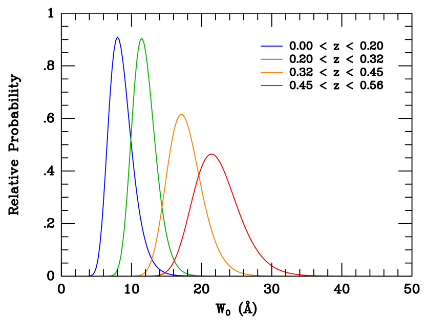
Figure 2.— Relative likelihoods that the rest-frame [O II] equivalent widths plotted in Figure 1 are drawn from an exponential distribution with scale length $W_{0}$. Objects with equivalent widths less than 5 Å have been excluded from the fit. In the local universe, rest-frame [O II] equivalent widths e-fold with a scale length of $\sim 8$ Å; by $z\sim 0.5$, this scale length has increased to $\sim 22$ Å.

5. Internal Extinction within the Sample

Before we can translate the HETDEX [O II] luminosities into star formation rates, we must first examine the effect that internal extinction has on each galaxy’s emergent emission-line flux. Often times, this is done by applying a mean reddening correction to the population of galaxies as a whole (e.g., Fujita et al., 2003; Ly et al., 2007); in other cases, a mean extinction is defined as a function of galaxy absolute magnitude (e.g., Moustakas et al., 2006; Zhu et al., 2009). However, a more robust way of handling the problem is to de-redden each galaxy individually using information from the galaxy itself. Although the HETDEX spectra lack sufficient wavelength coverage to constrain internal extinction via the Balmer decrement, all of the survey fields have been imaged in a variety of bandpasses, from the UV (with GALEX) through the near-IR. Thus, it is possible to obtain an estimate of each object’s internal extinction by fitting its spectral energy distribution (SED) to models of galactic evolution.

To do this, we used the population synthesis code of Bruzual & Charlot (2003) to create a three-dimensional grid of models using the assumptions of solar-metallicity stellar evolution (Bressan et al., 1993), a Salpeter (1955) initial mass function, and a Calzetti (2001) reddening law. In total, 504 models were produced, using four different values for the e-folding timescale of star formation ($\tau=$10, 50, 100, and 500 Myr), 21 logarithmically spaced galactic ages ($1{\rm\ Myr}<t<10$ Gyr), and six uniformly spaced values for the stellar reddening ($0<E(B-V)<0.5$). We then found the best-fitting values of $\tau,t$, and $E(B-V)$ by fitting each galaxy’s observed multicolor photometry to the computed colors of the grid via a $\chi^{2}$ minimization code. Obviously, single-component population synthesis models such as these are somewhat limited, as they cover only a small part of galaxy parameter space. Nevertheless, the models do provide some guidance as to a galaxy’s internal extinction, and therefore represent an important improvement in the study of the evolution of star formation.

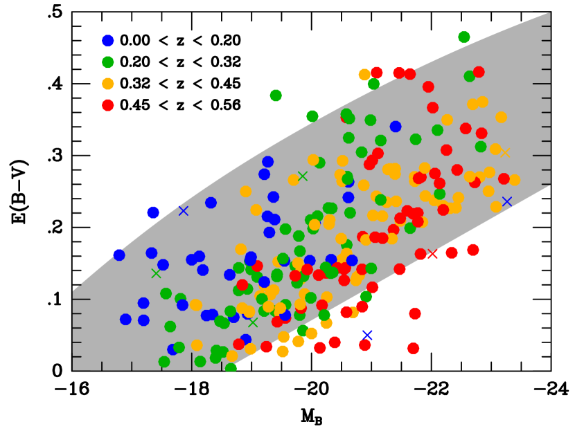
Figure 3.— SED-based stellar reddening values for the 259 VIRUS-P [O II] emitting galaxies above the 80% completeness limit, as a function of function of galaxy absolute magnitude. The grey area approximates the locus of points found by Moustakas et al. (2006) using the Balmer decrements of a local sample of galaxies. The agreement between the two samples is excellent, and there is no evidence for a redshift dependence in the extinction. The crosses represent seven probable AGN.

Figure 3 shows the SED-based stellar reddenings for our sample of [O II] emitters, as a function of galactic absolute magnitude and redshift. For the figure, we have adopted the extinction curve of Calzetti (2001), along with the relation

$$E(B-V)_{\rm stars}=0.44E(B-V)_{\rm gas}$$ (1)

which Calzetti (2001) inferred from UV, far-IR, and Balmer-line observations of $\sim 50$ starburst galaxies in the local neighborhood. The figure confirms the well-known correlation between a galaxy’s absolute magnitude and extinction (e.g., Wang & Heckman, 1996; Tully et al., 1998; Jansen et al., 2001). Indeed, the use of equation (1) recovers the relation observed by Moustakas et al. (2006) for galaxies in the local neighborhood. Also, this is no clear evidence for a shift in the relation with redshift, although the size of the dispersion ($\sigma_{E(B-V)}\sim 0.2$), the limited number of objects, and the dependence of survey volume and completeness on redshift all conspire to make measurements of the evolution of extinction difficult. The full sample of $\sim 10^{6}$ HETDEX galaxies will greatly improve upon this situation (Hill et al., 2008a).

Another test of the robustness of our reddening estimates is to compare the de-reddened [O II] $\lambda 3727$ luminosities with the galaxies’ de-reddened near-UV magnitudes, as recorded in the GR6 catalog of GALEX (Martin et al., 2005). Both datasets probe the presence of hot, young stars: [O II] through the indirect detection of ionizing radiation, and the UV via the direct measurement of the stellar continuum of hot stars. However, according to the Calzetti (2001) extinction law, the extinction that effects [O II] $\lambda 3727$ emission line is $\sim 3.5$ times greater than that which extinguishes a galaxy’s UV continuum. Consequently, any systematic error in our reddening estimates should be easily visible in a comparison of the inferred star formation rates.

To perform this test, we used the UV continuum star formation rate calibration of Kennicutt (1998)

$${\rm SFR(UV)}(M_{\odot}~{}{\rm yr}^{-1})=1.4\times 10^{-28}\,L_{\nu}\ ({\rm ergs~{}s}^{-1}{\rm Hz}^{-1})$$ (2)

and the empirical [O II] $\lambda 3727$ calibration of Kewley et al. (2004)

$${\rm SFR([O~{}II])}(M_{\odot}~{}{\rm yr}^{-1})=6.58\times 10^{-42}\,L({\rm[O~{}II]})\ ({\rm ergs~{}s}^{-1})$$ (3)

Both of these calibrations assume a Salpeter (1955) initial mass function truncated at $100M_{\odot}$ and present-day solar metallicity. (Because of our limited wavelength coverage, no $R_{23}$ abundance correction could be applied to the [O II] luminosities.) If our reddening estimates are robust, and if the Calzetti (2001) extinction law holds, the ratio of these two star formation rate indicators should be one.

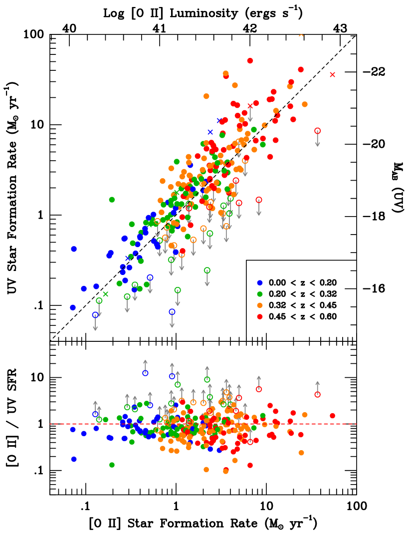
Figure 4.— A comparison of star formation rates derived from measurements of the UV continuum (using the calibration of Kennicutt, 1998) and [O II] flux (via the calibration of Kewley et al. (2004) without the $R_{23}$ correction for oxygen abundance). The UV fluxes have been $k$-corrected, and both quantities have been corrected for internal extinction via our SED-based reddening values and a Calzetti (2001) reddening law. Open circles mark objects that are not in the GALEX GR6 catalog, and denote approximate upper limits. The crosses show X-ray bright objects. The scatter in the diagram is substantial, but any systematic error between the two SFR indicators is small.

Figure 4 performs this comparison. In the figure, an SED-based $k$-correction has been applied to the GALEX near-UV magnitudes, and both quantities have been corrected for internal extinction using the Calzetti (2001) reddening law. From the figure, it is clear that the two star formation indicators are strongly correlated. The best-fit slope of the relation, as determined by the Buckley-James and EM algorithms for censored data (see Isobe et al., 1986), is just slightly less than one ($0.95\pm 0.04$), with the offset in the direction predicted by Kewley et al. (2004) for high star formation rate systems. Interestingly, the scatter about this line, ($\sigma\sim 0.3$ dex) is three times larger than the typical $\sim 0.1$ dex errors associated with our [O II] and UV measurements, and significantly greater than the $\sim 0.08$ dex dispersion seen in local comparisons of H$\alpha$ and [O II] star formation rates (e.g., Kewley et al., 2004). Part of this scatter is likely due to our use of the mean Kewley et al. (2004) calibration for [O II] emission; without spectral measurements at [O III] $\lambda 5007$ and H$\beta$, we cannot apply second-order corrections to compensate for the ionization state and oxygen abundance of the gas. In addition, the extinction that affects the forbidden [O II] emission line is not necessarily that which extinguishes the UV continuum: while equation (1) works well in the mean, there should be a non-negligible amount of dispersion about this relation. Thus, even if our SED-based extinction estimates were perfect, our error budget would still have this additional reddening term. Finally, some component of the scatter may be driven by the stochastic nature of star formation. Emission-line SFR indicators, such as H$\alpha$ and [O II] $\lambda 3727$, record star formation over the past $\sim 20$ Myr, while measurements of the stellar UV continuum probe a timescale that is $\sim 5$ times longer (Kennicutt, 1998). The scatter between the two indicators must necessarily be larger than that seen in an H$\alpha$-[O II] comparison. In any case, the figure confirms that our estimates for internal reddening are reasonable and should not inject any large systematic effects into our analysis.

6. The [O II] Emission-Line Luminosity Function

To measure the [O II] emission-line luminosity function, we began by following the procedures described in Blanc et al. (2011) and applied the $1/V_{\rm max}$ technique (Schmidt, 1968; Huchra & Sargent, 1973) to the 360 separate dithered pointings of the HETDEX pilot survey. As described in Adams et al. (2011), the noise characteristics of each survey frame were recorded as a function of wavelength. Consequently, for each [O II] emitter in the sample, we could calculate $V_{\rm max}$, the co-moving volume of all redshifts at which the object could have been detected with a signal-to-noise ratio above a given threshold. The implied number density of galaxies in any absolute luminosity bin, $d\log L$, is then

$$\phi(\log L)={1\over\Delta(\log L)}\eta\,\sum_{i}\left\{{1\over V_{\rm max}(i)}\right\}$$ (4)

where $\eta$ is the inverse of the completeness function, and the summation is performed over all galaxies with luminosities falling within the bin. Figure 5 displays these derived [O II] luminosity functions (both observed and de-reddened) for the redshift intervals $0<z<0.2$, $0.2<z<0.325$, $0.325<z<0.45$ and $0.45<z<0.56$. In each panel, we have excluded the likely AGN (3 objects in panels 1, 2, and 4, and 1 object in panel 3), binned the data into $\Delta\log L=0.2$ intervals, and drawn error bars based on the bin’s counting statistics.

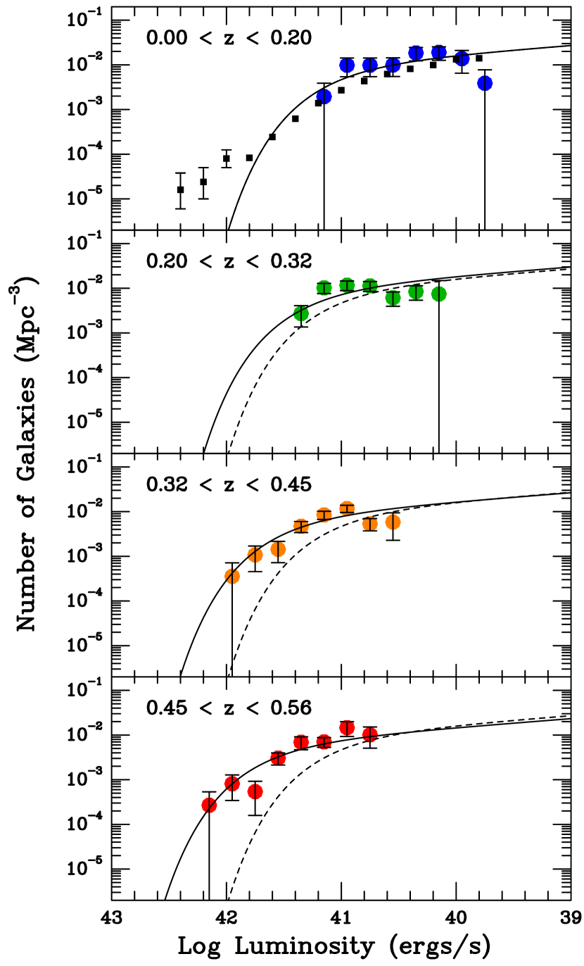
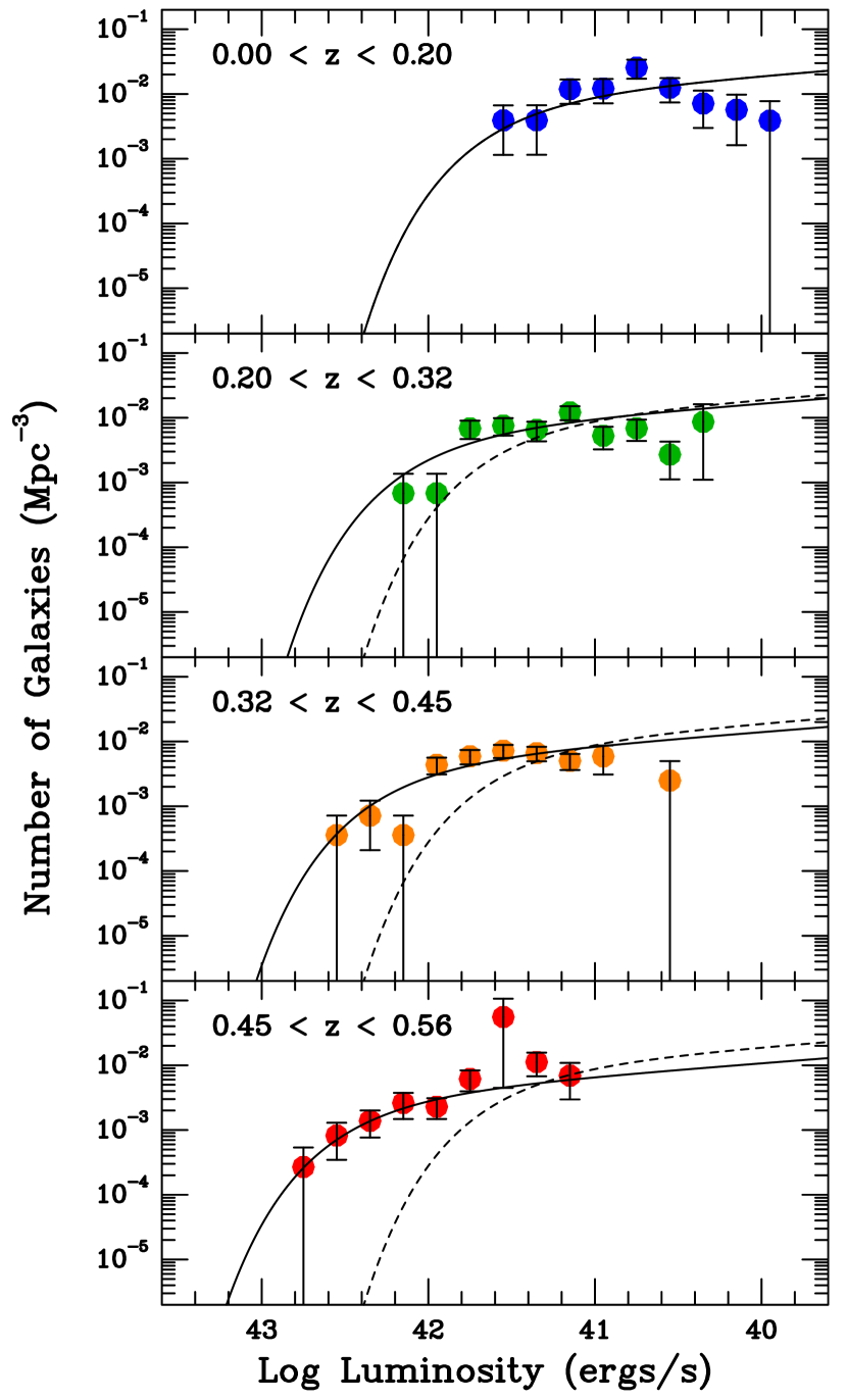
Figure 5.— The observed (left) and de-reddened (right) [O II] $\lambda 3727$ luminosity functions as a function of redshift. The black points in the left-hand diagram display the local luminosity function of Gilbank et al. (2010). The dashed curves show the best-fit Schechter (1976) function for the lowest redshift bin, while the solid lines show the best-fit functions at each redshift. In both plots, the faint-end slope of the fitted luminosity functions has been fixed at $\alpha=-1.2$. While there is evolution in both functions, the change of $L^{*}$ with redshift is much more pronounced when reddening is taken into account.

As can be seen from the top segments of the figure, our $z<0.2$ observed luminosity function is in very good agreement with that derived for $z<0.2$ galaxies in SDSS Stripe 82 (Gilbank et al., 2010). In this lowest redshift bin, our survey volume is only $\sim 2600$ Mpc³, hence intrinsically rare objects which populate the extreme bright-end of the luminosity function are poorly represented. However, at fainter line-luminosities our function is reasonably well-fixed at a level that is $\sim 40\%$ higher than that found by Gilbank et al. (2010). This is consistent with the expectations, as for the galactic number densities under consideration, the effects of cosmic variance should be of this order (Trenti & Stiavelli, 2008).

At redshifts $z>0.2$, there is clear evidence for evolution, both in the observed luminosity function and, more dramatically in the de-reddened function. To quantify these changes, we fit the data of Figure 5 to a Schechter (1976) function, i.e.,

$$\phi(L/L^{*})d(L/L^{*})=\phi^{*}\left(L/L^{*}\right)^{\alpha}e^{-L/L^{*}}d(L/L^{*})$$ (5)

and examined the behavior of $L^{*}$ and $\phi^{*}$ as a function of redshift. While other forms of the luminosity function are possible – both Zhu et al. (2009) and Gilbank et al. (2010) use double power laws for their [O II] datasets – our sample of objects is not large enough to warrant the introduction of additional parameters into our analysis. Quantifying the evolution of the bright, intrinsically rare [O II] emitters requires a much larger survey volume, such as that which will be covered by the full HETDEX program.

To fit the luminosity functions of Figure 5, we avoided the limitations associated with our finite-sized bins, and used a maximum-likelihood analysis. We began by computing $\phi^{\prime}(L)$, the true luminosity function (in galaxies per cubic Megaparsec) from which the data of Figure 5 are drawn, modified by observational selection effects, such as photometric errors and incompleteness. By definition, in a given volume of the universe, $\Delta V$, and within a given luminosity interval, $\Delta L$, we should expect to observe $\lambda=\phi^{\prime}(L)\Delta L\,\Delta V$ galaxies. From simple Poisson statistics, the probability of actually observing $n$ galaxies in that same interval is

$$p(n|\lambda)={\lambda^{n}e^{-\lambda}\over n!}$$ (6)

If we shrink the bin size down to zero so that the interval becomes a differential, then each division of the luminosity function will contain either zero or one object. The probability of observing any given luminosity function is then

$$P = \displaystyle\prod_{\rm bins\ with\ 0}{\lambda_{i}^{0}e^{-\lambda_{i}}\over 0!}\ \cdot\ \prod_{\rm bins\ with\ 1}{\lambda_{i}^{1}e^{-\lambda_{i}}\over 1!}$$ (7)

$$= \displaystyle\prod_{\rm all\ bins}e^{-\lambda_{i}}\ \cdot\ \prod_{i=1}^{N}\lambda_{i}$$

where $N$ is the total number of galaxies observed. With a little manipulation, this becomes

$$P=\exp\left\{-\sum\phi^{\prime}(L)dL\,dV\right\}\,\prod_{i=1}^{N}\phi^{\prime}(L_{i})dL\,dV$$ (8)

or, in terms of relative log likelihoods

$$\ln P=-\int_{z_{1}}^{z_{2}}\int_{L_{\rm min}(z)}^{\infty}\phi^{\prime}(L)dL\,dV+\sum_{i}^{N}\ln\phi^{\prime}(L_{i})$$ (9)

where $L_{\rm min}$ is the luminosity limit of the survey at redshift $z$. The function $\phi^{\prime}(L)$ was then varied to map out the distribution of likelihoods as a function of $\log L^{*}$, $\alpha$, and the mean density of galaxies brighter than given line luminosity. Note that this style of analysis is similar to the classical method of Sandage et al. (1979), with the double integral term providing the normalization for $\phi$ (Drory et al., 2003).

Figure 6.— Likelihood contours of our Schechter (1976) fits to the observed [O II] $\lambda 3727$ emission-line luminosity functions for our four redshift bins. The contours are drawn at $0.5\,\sigma$ intervals from $0.5\,\sigma$ to $3\,\sigma$. The left-hand panels marginalize over normalization and show probability versus $\log L^{*}$ and $\alpha$; the right-hand panels marginalize over $\alpha$, and plot likelihoods versus $\log L^{*}$ and the integral of the Schechter function. (The latter parameter is less dependent on $\alpha$ and $L^{*}$.) Note the increase in $L^{*}$ with redshift and the poorly constrained measurement of $\alpha$.

Figure 6 shows the likelihood contours for the observed luminosity function. The left-hand panels marginalizes over the integral of the luminosity function (which serves as a proxy for $\phi^{*}$) and shows the probabilities as a function of $\alpha$ and $\log L^{*}$; the right-hand side marginalizes over $\alpha$. The first feature to notice is that the faint-end slope of our function is poorly defined; this is a natural consequence of the limited number of objects in our sample. Literature estimates of $\alpha$ vary substantially, from $\alpha=-1.2$ (Gallego et al., 2002) to $\alpha=-1.6$ (Sullivan et al., 2000), but our data imply slopes that are even shallower. However, this result is quite sensitive to the incompleteness corrections which have been applied to the measurements near the $\sim 5\,\sigma$ detection limits. For the discussion that follows, we fix $\alpha=-1.2$, while noting that shallower (or steeper) slopes cannot be excluded.

Table 1 lists of best-fitting values of $L^{*}$ and $\phi^{*}$ under the assumption that $\alpha=-1.2$. These fits are also displayed in the left-hand panel of Figure 5. In the two lowest redshift bins ($z<0.325$) where our survey volume is relatively small, the bright-end of the luminosity function is sparsely populated, and the exact location of $L^{*}$ is defined as much by our assigned value of $\alpha$ and by the absence of luminous objects as the presence of $L>L^{*}$ galaxies. Nevertheless, the exponential cutoff in the lowest redshifts bins is reasonably well-defined with $\log L^{*}=41.07\pm 0.17$ at $z<0.2$ and $\log L^{*}=41.29\pm 0.11$ at $0.2<z<0.325$. These values are significantly fainter than those measured in the higher redshift bins, where our survey volume is larger, and the knees of the luminosity functions are better populated. Overall, the data imply an increase in $L^{*}$ of $\sim 1.5$ mag per unit redshift over the redshift limits of our survey.

Figure 7.— Likelihood contours of our Schechter (1976) fits to the de-reddened [O II] $\lambda 3727$ emission-line luminosity functions for our four redshift bins. No correction for galaxies extinguished below the survey’s completeness limit has been applied. The contours are drawn at $0.5\,\sigma$ intervals from $0.5\,\sigma$ to $3\,\sigma$. The left-hand panels marginalize over normalization and show probability versus $\log L^{*}$ and $\alpha$; the right-hand panels marginalize over $\alpha$, and plot likelihoods versus $\log L^{*}$ and the integral of the Schechter function. Because extinction correlates with luminosity, the evolution of $L^{*}$ with redshift is more dramatic than for the observed luminosity function.

Figure 7 shows the results of our maximum-likelihood fits after de-reddening the [O II] $\lambda 3727$ line-luminosity of each galaxy using our SED-based extinction values. Predictably, the evolution of $L^{*}$ with redshift is stronger than for the raw luminosity function. As pointed out by a number of authors (e.g., Wang & Heckman, 1996; Hopkins et al., 2001; Ly et al., 2012), the amount of extinction affecting a galaxy’s emission lines strongly correlates with its star formation rate, with more active galaxies possessing more internal extinction. Consequently, as the knee of the observed luminosity function shifts towards brighter values, the amount of internal reddening increases, leading to a larger shift in the de-reddened value of $L^{*}$. At $z<0.2$, the difference between the best-fitting observed and de-reddened values of $L^{*}$ is $\Delta\log L^{*}=0.4\pm 0.2$ dex; by $z\sim 0.5$, this offset becomes at least $\Delta\log L^{*}=0.7\pm 0.2$ dex. The brightening of $L^{*}$ with redshift increases the importance of internal reddening, and explains why our de-reddened values for $L^{*}$ are brighter than those of Ly et al. (2007), who used a mean reddening correction for all the galaxies in their $z\sim 1$ survey.

We do note that our de-reddened luminosity function displayed in the right-hand panel of Figure 5 is almost certainly an underestimate. While one can count the observed number of galaxies in some interval about a de-reddened luminosity $L_{0}$, there is always the possibility that some additional galaxies which belong in the interval are extincted below the flux limit of the survey. Obviously, the problem becomes more serious at fainter magnitudes, but at higher redshifts, even relatively bright galaxies may be missing from the data.

To examine the possible importance of this effect, we can use the MPA-JHU spectrum measurements of galaxies in the SDSS Data Release 7. This catalog contains the line fluxes and Balmer-line extinction estimates for several hundred thousand galaxies in the nearby universe, allowing us to examine the distribution of [O II] extinctions as a function of intrinsic [O II] luminosity. These data illustrate a smooth trend in both the mean extinction of a population and the dispersion about this mean. For example, for systems with [O II] luminosities of $\sim 10^{39}$ ergs s^-1, the mean extinction is $E(B-V)\sim 0.2$ with a dispersion of $\sigma_{E(B-V)}\sim 0.13$ about this mean. By $L([O~{}II])\sim 10^{43}$ ergs s^-1 however, $\langle E(B-V)\rangle$ has increased to $\sim 0.75$ and the dispersion has increased to $\sigma_{E(B-V)}\sim 0.36$. If this relation holds through $z\sim 0.5$, then, at any luminosity and distance, we could, at least in theory, compute the fraction of galaxies that should be extinguished below our completeness limit, and include that as an additional factor in the computation of the modified luminosity function $\phi^{\prime}(L)$.

Unfortunately, the current sample of galaxies is not extensive enough to apply this analysis technique or test the validity of our assumptions about extinction. To study galaxies beyond the knee of the $z>0.4$ [O II] $\lambda 3727$ luminosity function, one must reach intrinsic [O II] luminosities of $\sim 10^{41}$ ergs s^-1. Such objects have a mean internal extinction of $E(B-V)\sim 0.4$, but with a dispersion of $\sigma_{E(B-V)}\sim 0.15$ about this mean. Consequently, in order to keep the incompleteness corrections below $\sim 50\%$, one must reach observed [O II] luminosities of $\sim 10^{40}$ ergs s^-1, and exclude detections within $\sim 1$ dex of the frame limit. At redshifts $z\gtrsim 0.3$, our current data do not have a sufficient number of galaxies to satisfy this criteria. The full HETDEX survey will certainly be able to investigate this question.

7. Evolution of the Star Formation Rate Density

For individual galaxies, the relationship between [O II] luminosity and star formation rate is complicated, since it depends on variables such as extinction, metallicity, and excitation. However, relatively robust calibrations for galaxy ensembles do exist in the literature (Jansen et al., 2001; Kewley et al., 2004; Moustakas et al., 2006), and these can be used to translate our [O II] luminosity functions into star formation rate densities. As Figure 4 illustrates, the Kewley et al. (2004) relation (without its second-order metallicity correction) gives star formation rates that are reasonably consistent with measurements in the UV. This is the conversion we adopt for our study.

Table 1 lists two estimates for the [O II] $\lambda 3727$ star formation rate density: one derived by extrapolating a faint-end slope of $\alpha=-1.2$ to infinity and applying a single mean extinction of $A_{3727}=1.88$ mag to all galaxies (Hopkins, 2004; Takahashi et al., 2007), and a second using the same faint-end extrapolation, but with our individual extinction estimates. (Our luminosity functions are sufficiently deep that this extrapolation only increases the observed SFRD by $\sim 10\%$.) In general, the SFRDs derived from the individual reddening values are $\sim 0.3$ dex smaller than those inferred using a mean extinction. This should not be too surprising: while the latter method more accurately corrects for extinction at the bright end of the luminosity function, it most likely underestimates the function’s faint-end slope, due to the contribution of galaxies whose internal extinction causes them to fall out of our sample. Conversely, the application of a mean extinction likely overestimates the faint-end slope, since the $E(B-V)$ correlates directly with line luminosity. A steepening of $\alpha$ by just $\sim-0.4$ would move the two values into agreement.

Figure 8 compares our individually de-reddened SFRDs to other emission-line based SFRDs, using the calibrations of Kennicutt (1998) for H$\alpha$, Kewley et al. (2004) for [O II] $\lambda 3727$, and Ly et al. (2007) for [O III] $\lambda 5007$. Clearly, the diagram has quite a bit of scatter, in part due to the different assumptions investigators make about internal extinction. Nevertheless, the well-known correlation between star formation rate density and redshift is easily seen, and our data agree with those of most other measurements of instantaneous star formation rate. At $z\sim 0.5$, our value of $\rho_{\rm SFRD}=3.4^{+1.3}_{-1.1}\times 10^{-2}M_{\odot}$ yr^-1 Mpc^-3 is $\sim 4$ times greater than that seen in the local ($z<0.2$) universe, yet a factor of $\sim 2$ below that inferred from [O II] observations at $z\sim 1$. Our data populate the gap between the [O II] measurements in the local and high-redshift universe.

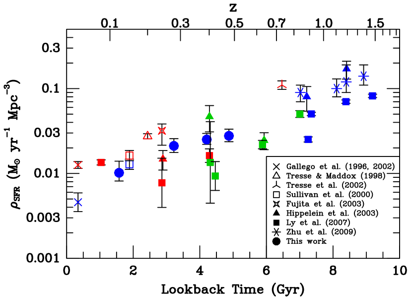
Figure 8.— Extinction-corrected measurements of the cosmic star formation rate density based on the emission-lines of H$\alpha$ (in red), [O III] $\lambda 5007$ (in green) and [O II] $\lambda 3727$ (in blue). The circles show the data from this paper. Included in the plot are measurements from the literature using the calibrations of Kennicutt (1998) for H$\alpha$, Kewley et al. (2004) for [O II] $\lambda 3727$, and Ly et al. (2007) for [O III] $\lambda 5007$.

8. Conclusions

We have used the sample of 284 [O II]-selected galaxies from the HETDEX pilot survey to explore evolution in star formation over the last $\sim 5$ Gyr of cosmic time. By analyzing the distribution of HETDEX line fluxes, we find that, over the redshift range $0<z<0.56$, the observed [O II] luminosity function exhibits significant evolution, with $\log L^{*}$ fading by $\sim 0.4$ dex between $z\sim 0.5$ and $z\sim 0$. However, this shift tells only part of the story. Because the HETDEX pilot survey was conducted in areas of the sky with large amounts of ancillary data, we used each galaxy’s spectral energy distribution to estimate its internal reddening. By adopting these stellar $E(B-V)$ measurements, and assuming $E(B-V)_{\rm stars}=0.44\,E(B-V)_{\rm gas}$ (Calzetti, 2001), we were able to correct each galaxy’s observed [O II] flux for internal extinction, and thereby obtain an estimate of its intrinsic [O II] luminosity. The resultant extinction-corrected luminosity function exhibits stronger evolution in $\log L^{*}$ than the observed function, with this characteristic luminosity fading by $\sim 1.3$ mag between $z\sim 0.5$ and today. The difference between the observed and de-reddened functions is consistent with the expectation that galaxies with higher star formation rates have greater internal extinction.

A similar evolutionary trend is seen in the strength of the [O II] line relative to the continuum. While the distribution of rest-frame [O II] equivalent width is insensitive to line-luminosity, it does depend strongly on redshift. Specifically, there are many more high-equivalent width [O II] emitters at $z\sim 0.5$ than there are today. If we exclude the weak line emitters (i.e., those objects with rest-frame equivalent widths less than 5 Å) and fit an exponential to the remainder of the distribution, then we find that the scale length of rest-frame equivalent widths decreases smoothly, from $W_{0}=22\pm 3$ Å at $z>0.45$ to $W_{0}=8\pm 2$ Å at $z<0.2$. This reddening-independent measure of star formation confirms that the relative intensity of galactic starbursts has been decreasing over the last $\sim 5$ Gyr.

By integrating our extinction-corrected [O II] luminosity functions and using the [O II] SFR calibration of Kewley et al. (2004), we derive the star formation rate density in four redshift bins. We find that the SFRD decreases linearly with time, changing by a factor of $\sim 4$ between $z\sim 0.5$ and today. Our data cover the gap between the [O II] observations of the local universe and those at $z\sim 1$, and are in excellent agreement with measurements based on the H$\alpha$ and [O III] $\lambda 5007$ line. There remains a substantial amount of scatter in the SFRD diagram, but this is due in large part to differences in techniques and reddening assumptions. Our analysis, which employs individual SED-based reddening estimates and spans the redshift range $0<z<0.5$, removes some of these problems.

The sample presented here highlights the power of the upcoming HETDEX survey (Hill et al., 2008a) to open up the emission-line universe. HETDEX will map out over 300 deg² of sky with a blind, integral-field spectroscopic survey. While the main goal of the project is to measure the power spectrum of $\sim 800,000$ Ly$\alpha$ emitting galaxies between $1.9<z<3.5$ and measure the evolution of the dark energy equation of state, the survey will also identify $\sim 10^{6}$ $z<0.5$ [O II] emitters. This unprecedented large sample of emission-line galaxies will cover the entire range of galactic environments and allow us to trace the evolution of star formation in field galaxies and clusters over the last $\sim 5$ Gyr of cosmic time.

Table 1Best-Fit Schechter Function Parameters

			Observed			Extinction-Corrected
		$W_{0}$	$\log L^{*}$	$\log\phi(>40.5)$	$\log\rho_{\rm SFRD}$	$\log L^{*}$	$\log\phi(>40.5)$	$\log\rho_{\rm SFRD}$
$z$	$N_{\rm obj}$	(Å)	(ergs s-1)	(Mpc-3)	($M_{\odot}$ yr-1 Mpc-3)	(ergs s-1)	(Mpc-3)	($M_{\odot}$ yr-1 Mpc-3)
0.000 – 0.200	39	$8.0\pm 1.6$	$41.07^{+0.18}_{-0.16}$	$-2.30^{+0.09}_{-0.11}$	$-1.63\pm 0.11$	$41.48^{+0.21}_{-0.13}$	$-2.02^{+0.07}_{-0.08}$	$-1.99\pm 0.11$
0.200 – 0.325	70	$11.5\pm 1.6$	$41.29^{+0.11}_{-0.11}$	$-2.12^{+0.05}_{-0.06}$	$-1.40\pm 0.06$	$41.96^{0.12}_{-0.12}$	$-1.92^{+0.04}_{-0.05}$	$-1.67\pm 0.08$
0.325 – 0.450	89	$16.6\pm 2.4$	$41.50^{+0.08}_{-0.10}$	$-2.07^{+0.04}_{-0.05}$	$-1.29\pm 0.05$	$42.16^{0.10}_{-0.11}$	$-1.95^{+0.03}_{-0.05}$	$-1.60\pm 0.06$
0.450 – 0.560	76	$21.5\pm 3.3$	$41.68^{+0.08}_{-0.12}$	$-2.07^{+0.03}_{-0.08}$	$-1.24\pm 0.06$	$42.36^{0.11}_{-0.12}$	$-2.02^{+0.04}_{-0.07}$	$-1.56\pm 0.07$

References

- Adams et al. (2011) Adams, J.J., Blanc, G.A., Hill, G.J., Gebhardt, K., Drory, N., Hao, L., Bender, R., Byun, J., Ciardullo, R.. Cornell, M.E., Finkelstein, S.L., Fry, A., Gawiser, E., Gronwall, C., Hopp, U., Jeong, D., Kelz, A., Kelzenberg, R., Komatsu, E., MacQueen, P.J., Murphy, J., Odoms, P.S., Roth, M., Schneider, D.P., Tufts, J.R., & Wilkinson, C.P. 2011, ApJS, 192, 5
- Baldwin et al. (1981) Baldwin, J.A., Phillips, M.M., & Terlevich, R. 1981, PASP, 93, 5
- Blanc et al. (2011) Blanc, G.A., Adams, J., Gebhardt, K., Hill, G.J., Drory, N., Hao, L., Bender, R., Ciardullo, R., Finkelstein, S.L., Gawiser, E., Gronwall, C., Hopp, U., Jeong, D., Kelzenberg, R., Komatsu, E., MacQueen, P., Murphy, J.D., Roth, M.M., Schneider, D.P., & Tufts, J. 2011, ApJ, 736, 31
- Blanton & Lin (2000) Blanton, M., & Lin, H. 2000, ApJ, 543, L125
- Bouwens et al. (2010) Bouwens, R.J., Illingworth, G.D., Oesch, P.A., Stiavelli, M., van Dokkum, P., Trenti, M., Magee, D., Labbé, I., Franx, M., Carollo, C.M., & Gonzalez, V. 2010, ApJ, 709, L133
- Bressan et al. (1993) Bressan, A., Fagotto, F., Bertelli, G., & Chiosi, C. 1993, A&AS, 100, 647
- Bruzual & Charlot (2003) Bruzual, G., & Charlot, S. 2003, MNRAS, 344, 1000
- Calzetti (2001) Calzetti, D. 2001, PASP, 113, 1449
- Drory et al. (2001) Drory, N., Feulner, G., Bender, R., Botzler, C.S., Hopp, U., Maraston, C., Mendes de Oliveira, C., & Snigula, J. 2001, MNRAS, 325, 550
- Drory et al. (2003) Drory, N., Bender, R., Feulner, G., Hopp, U., Maraston, C., Snigula, J., & Hill, G.J. 2003, ApJ, 595, 698
- Fujita et al. (2003) Fujita, S.S., Ajiki, M., Shioya, Y., Nagao, T., Murayama, T., Taniguchi, Y., Umeda, K., Yamada, S., Yagi, M., Okamura, S., & Komiyama, Y. 2003, ApJ, 586, L115
- Gallego et al. (1996) Gallego, J., Zamorano, J., Rego, M., Alonso, O., & Vitores, A.G. 1996, A&AS, 120, 323
- Gallego et al. (2002) Gallego, J., García-Dabó, C.E., Zamorano, J., Aragón-Salamanca, A., & Rego, M. 2002, ApJ, 570, L1
- Giavalisco et al. (2004) Giavalisco, M., Dickinson, M., Ferguson, H.C., Ravindranath, S., Kretchmer, C., Moustakas, L.A., Madau, P., Fall, S.M., Gardner, J.P., Livio, M., Papovich, C., Renzini, A., Spinrad, H.. Stern, D., & Riess, A. 2004, ApJ, 600, L93
- Gilbank et al. (2010) Gilbank, D.G., Baldry, I.K., Balogh, M.L., Glazebrook, K., & Bower, R.G. 2010, MNRAS, 405, 2594
- Glazebrook et al. (2004) Glazebrook, K., Tober, J., Thomson, S., Bland-Hawthorn, J., & Abraham, R. 2004, AJ, 128, 2652
- Gronwall et al. (2007) Gronwall, C., Ciardullo, R., Hickey, T., Gawiser, E., Feldmeier, J.J., van Dokkum, P.G., Urry, C.M., Herrera, D., Lehmer, B.D., Infante, L., Orsi, A., Marchesini, D., Blanc, G.A., Francke, H., Lira, P., & Treister, E. 2007, ApJ, 667, 79
- Hammer et al. (1997) Hammer, F., Flores, H., Lilly, S.J., Crampton, D., Le Fèvre, O., Rola, C., Mallen-Ornelas, G., Schade, D., & Tresse, L. 1997, ApJ, 481, 49
- Hill et al. (2008a) Hill, G.J., Gebhardt, K., Komatsu, E., Drory, N., MacQueen, P.J., Adams, J., Blanc, G.A., Koehler, R., Rafal, M., Roth, M.M., Kelz, A., Gronwall, C., Ciardullo, R., & Schneider, D. 2008a, ASP Conf. Ser. 399, Panoramic Views of Galaxy Formation and Evolution, ed. T. Kodama, T. Yamada, & K. Aoki (San Francisco: Astronomical Society of the Pacific), 115
- Hill et al. (2008b) Hill, G.J., MacQueen, P.J., Smith, M.P., Tufts, J.R., Roth, M.M,; Kelz, A., Adams, J.J., Drory, N., Grupp, F., Barnes, S.I., Blanc, G.A., Murphy, J.D., Altmann, W., Wesley, G.L., Segura, P.R., Good, J.M., Booth, J.A., Bauer, S.-M., Popow, E., Goertz, J.A., Edmonston, R.D., & Wilkinson, C.P. 2008b, Proc. SPIE, 7014, 231
- Hippelein et al. (2003) Hippelein, H., Maier, C., Meisenheimer, K., Wolf, C., Fried, J.W., von Kuhlmann, B., Kümmel, M., Phleps, S., & Röser, H.-J. 2003, A&A, 402, 65
- Ho (2005) Ho, L.C. 2005, ApJ, 629, 680
- Hogg et al. (1998) Hogg, D.W., Cohen, J.G., Blandford, R., & Pahre, M.A. 1998, ApJ, 504, 622
- Hopkins et al. (2001) Hopkins, A.M., Connolly, A.J., Haarsma, D.B., & Cram, L.E. 2001, AJ, 122, 288
- Hopkins (2004) Hopkins, A.M. 2004, ApJ, 615, 209
- Hopkins & Beacom (2006) Hopkins, A.M., & Beacom, J.F. 2006, ApJ, 651, 142
- Huchra & Sargent (1973) Huchra, J., & Sargent, W.L.W. 1973, ApJ, 186, 433
- Isobe et al. (1986) Isobe, T., Feigelson, E.D., & Nelson, P.I. 1986, ApJ, 306, 490
- Jansen et al. (2001) Jansen, R.A., Franx, M., & Fabricant, D. 2001, ApJ, 551, 825
- Kelson & Holden (2010) Kelson, D.D., & Holden, B.P. 2010, ApJ, 713, L28
- Kennicutt (1998) Kennicutt, R.C., Jr. 1998, ARA&A, 36, 189
- Kewley et al. (2001) Kewley, L.J., Heisler, C.A., Dopita, M.A., & Lumsden, S. 2001, ApJS, 132, 37
- Kewley et al. (2004) Kewley, L.J., Geller, M.J., & Jansen, R.A. 2004, AJ, 127, 2002
- Lehmer et al. (2010) Lehmer, B.D., Alexander, D.M., Bauer, F.E., Brandt, W.N., Goulding, A.D., Jenkins, L.P., Ptak, A., Roberts, T.P. 2010, ApJ, 724, 559
- Lilly et al. (1996) Lilly, S.J., Le Fevre, O., Hammer, F., & Crampton, D. 1996, ApJ, 460, L1
- Ly et al. (2007) Ly, C., Malkan, M.A., Kashikawa, N., Shimasaku, K., Doi, M., Nagao, T., Iye, M., Kodama, T., Morokuma, T., & Motohara, K. 2007, ApJ, 657, 738
- Ly et al. (2012) Ly, C., Malkan, M.A., Kashikawa, N., Ota, K., Shimasaku, K., Iye, M., & Currie, T. 2012, ApJ, 747, L16
- Madau et al. (1996) Madau, P., Ferguson, H.C., Dickinson, M.E., Giavalisco, M., Steidel, C.C., & Fruchter, A. 1996, MNRAS, 283, 1388
- Martin et al. (2005) Martin, D.C., Fanson, J., Schiminovich, D., Morrissey, P., Friedman, P.G., Barlow, T.A., Conrow, T., Grange, R., Jelinsky, P.N., Milliard, B., Siegmund, O.H.W., Bianchi, L., Byun, Y.-I., Donas, J., Forster, K., Heckman, T.M., Lee, Y.-W., Madore, B.F., Malina, R.F., Neff, S.G., Rich, R.M., Small, T., Surber, F., Szalay, A.S., Welsh, B., & Wyder, T.K. 2005, ApJ, 619, L1
- Moustakas et al. (2006) Moustakas, J., Kennicutt, R.C., Jr., & Tremonti, C.A. 2006, ApJ, 642, 775
- Persic et al. (2004) Persic, M., Rephaeli, Y., Braito, V., Cappi, M., Della Ceca, R., Franceschini, A., & Gruber, D.E. 2004, A&A, 419, 849
- Pettini et al. (2001) Pettini, M., Shapley, A.E., Steidel, C.C., Cuby, J.-G., Dickinson, M., Moorwood, A.F.M., Adelberger, K.L., & Giavalisco, M. 2001, ApJ, 554, 981
- Pierre et al. (2004) Pierre, M., et al. 2004, J. Cosmology Astropart. Phys., 9, 11
- Pirzkal et al. (2012) Pirzkal, N., Rothberg, B., Ly, C., Malhotra, S., Rhoads, J.E., Grogin, N.A., Dahlen, T., Meurer, G.R., Walsh, J.R., Hathi, N.P., Cohen, S.H., Bellini, A., Holwerda, B.W., Straughn, A.N., & Mechtley, M. 2012, arXiv:1208.5535
- Rujopakarn et al. (2010) Rujopakarn, W., Eisenstein, D.J., Rieke, G.H., Papovich, C., Cool, R.J., Moustakas, J., Jannuzi, B.T., Kochanek, C.S., Rieke, M.J., Dey, A., Eisenhardt, P., Murray, S.S., Brown, M.J.I., & Le Floc’h, E. 2010, ApJ, 718, 1171
- Salpeter (1955) Salpeter, E.E. 1955, ApJ, 121, 161
- Sandage et al. (1979) Sandage, A., Tammann, G.A., & Yahil, A. 1979, ApJ, 232, 352
- Schechter (1976) Schechter, P. 1976, ApJ, 203, 297
- Schmidt (1968) Schmidt, M. 1968, ApJ, 151, 393
- Scholz & Stephens (1987) Scholz, F.W., & Stephens, M.A. 1987, J. Amer. Stat. Assoc., 82, 918
- Scoville et al. (2007) Scoville, N., Aussel, H., Brusa, M., Capak, P., Carollo, C.M., Elvis, M., Giavalisco, M., Guzzo, L., Hasinger, G., Impey, C., Kneib, J.-P., LeFevre, O., Lilly, S.J., Mobasher, B., Renzini, A., Rich, R.M., Sanders, D.B., Schinnerer, E., Schminovich, D., Shopbell, P., Taniguchi, Y., & Tyson, N.D. 2007, ApJS, 172, 1
- Somerville et al. (2012) Somerville, R.S., Gilmore, R.C., Primack, J.R., & Dominguez, A. 2012, MNRAS, 423, 1992
- Sullivan et al. (2000) Sullivan, M., Treyer, M.A., Ellis, R.S., Bridges, T.J., Milliard, B., & Donas, J. 2000, MNRAS, 312, 442
- Takahashi et al. (2007) Takahashi, M.I., Shioya, Y., Taniguchi, Y., Murayama, T., Ajiki, M., Sasaki, S.S., Koizumi, O., Nagao, T., Scoville, N.Z., Mobasher, B., Aussel, H., Capak, P., Carilli, C., Ellis, R.S., Garilli, B., Giavalisco, M., Guzzo, L., Hasinger, G., Impey, C., Kitzbichler, M.G., Koekemoer, A., Le Fèvre, O., Lilly, S.J., Maccagni, D., Renzini, A., Rich, M., Sanders, D.B., Schinnerer, E., Scodeggio, M., Shopbell, P., Smolčić, V., Tribiano, S., Ideue, Y., & Mihara, S. 2007, ApJS, 172, 456
- Teplitz et al. (2003) Teplitz, H.I., Collins, N.R., Gardner, J.P., Hill, R.S., Heap, S.R., Lindler, D.J., Rhodes, J., & Woodgate, B.E. 2003, ApJS, 146, 209
- Trenti & Stiavelli (2008) Trenti, M., & Stiavelli, M. 2008, ApJ, 676, 767
- Tresse & Maddox (1998) Tresse, L., & Maddox, S.J. 1998, ApJ, 495, 691
- Tresse et al. (2002) Tresse, L., Maddox, S.J., Le Fèvre, O., & Cuby, J.-G. 2002, MNRAS, 337, 369
- Tully et al. (1998) Tully, R.B., Pierce, M.J., Huang, J.-S., Saunders, W., Verheijen, M.A.W., & Witchalls, P.L. 1998, AJ, 115, 2264
- Veilleux & Osterbrock (1987) Veilleux, S., & Osterbrock, D.E. 1987, ApJS, 63, 295
- Wang & Heckman (1996) Wang, B., & Heckman, T.M. 1996, ApJ, 457, 645
- Zhu et al. (2009) Zhu, G., Moustakas, J., & Blanton, M.R. 2009, ApJ, 701, 86