Gluino-driven Radiative Breaking, Higgs Boson Mass, Muon $\mathbf{g-2}$, and the Higgs Diphoton Decay in SUGRA Unification

Abstract

We attempt to reconcile seemingly conflicting experimental results on the Higgs boson mass, the anomalous magnetic moment of the muon, null results in search for supersymmetry at the LHC within the 8$\,\mathrm{Te\kern-0.80002ptV}$ data and results from $B$-physics, all within the context of supersymmetric grand unified theories. Specifically, we consider a supergravity grand unification model with non-universal gaugino masses where we take the $\mathrm{SU}(3)_{C}$ gaugino field to be much heavier than the other gaugino and sfermion fields at the unification scale. This construction naturally leads to a large mass splitting between the slepton and squark masses, due to the mass splitting between the electroweak gauginos and the gluino. The heavy Higgs bosons and Higgsinos also follow the gluino toward large masses. We carry out a Bayesian Monte Carlo analysis of the parametric space and find that it can simultaneously explain the large Higgs mass, and the anomalous magnetic moment of the muon, while producing a negligible correction to the Standard Model prediction for $\mathcal{B}r\left(B^{0}_{s}\to\mu^{+}\mu^{-}\right)$. We also find that the model leads to an excess in the Higgs diphoton decay rate. A brief discussion of the possibility of detection of the light particles is given. Also discussed are the implications of the model for dark matter.

I Introduction

The CMS and ATLAS collaborations have discovered and measured CMS:2012ufa ; ATLAS:2012tfa ; CMS:2012nga ; ATLAS:2012oga ; CMS:2013lba the mass of a new boson which is most likely the Higgs boson Englert:1964et ; Higgs:1964ia ; Higgs:1964pj ; Guralnik:1964eu responsible for breaking electroweak symmetry. In supersymmetry, one would identify this as the light $CP$-even Higgs boson Akula:2011aa ; Baer:2011ab ; Arbey:2011ab ; Draper:2011aa ; Carena:2011aa ; Akula:2012kk ; Strege:2012bt , $h^{0}$. Both experiments agree that the mass is between 125 and 126$\,\mathrm{Ge\kern-0.80002ptV}$. It is quite remarkable that the observed Higgs boson mass lies close to the upper limit predicted in grand unified supergravity models Chamseddine:1982jx ; Nath:1983aw ; Hall:1983iz ; Arnowitt:1992aq which is roughly 130$\,\mathrm{Ge\kern-0.80002ptV}$ Akula:2011aa ; Akula:2012kk ; Arbey:2012dq ; Ellis:2012aa ; Buchmueller:2011ab ; Baer:2012mv . (For a recent review of Higgs and supersymmetry see Nath:2012nh .) Because the mass of the $h^{0}$ boson in supersymmetry Nath:1983fp ; Carena:2002es ; Djouadi:2005gj is less than that of the $Z$ boson at the tree level, a large loop correction is necessary to match the measured value. The dominant one-loop Higgs self energy correction arises from its coupling to the top supermultiplet so that

$$\Delta m_{h^{0}}^{2}\simeq\frac{3m_{t}^{4}}{2\pi^{2}v^{2}}\ln\frac{M_{\rm S}^{2}}{m_{t}^{2}}+\frac{3m_{t}^{4}}{2\pi^{2}v^{2}}\left(\frac{X_{t}^{2}}{M_{\rm S}^{2}}-\frac{X_{t}^{4}}{12M_{\rm S}^{4}}\right)~{},$$ (1)

where $v=246\,\mathrm{Ge\kern-0.80002ptV}$, $M_{\mathrm{S}}$ is the average stop mass, $X_{t}=A_{t}-\mu\cot\beta$, $\mu$ is the Higgs mixing parameter and $A_{t}$ is the trilinear coupling (both at the electroweak scale), and $\tan\beta=\langle H_{2}\rangle/\langle H_{1}\rangle$, where $H_{2}$ gives mass to the up quarks while $H_{1}$ gives mass to the down quarks and leptons. Since $\Delta m_{h^{0}}^{2}$ has a logarithmic dependence of $M_{\mathrm{S}}$, a sizable $\Delta m_{h^{0}}^{2}$ correction implies that the scale $M_{\mathrm{S}}$ is high, lying in the several $\mathrm{Te\kern-0.80002ptV}$ region.

A high SUSY scale is also suggested by the ATLAS and CMS collaborations. So far, the LHC has delivered 5.3$\,\mathrm{fb}^{-1}$ and 23$\,\mathrm{fb}^{-1}$ of integrated luminosity lhcluminosity at 7$\,\mathrm{Te\kern-0.80002ptV}$ and 8$\,\mathrm{Te\kern-0.80002ptV}$ respectively to both CMS and ATLAS. Analysis of large portions of this data in search of supersymmetry has only yielded null results, though it is important to note that the parametric exclusion limits provided are typically only on minimal or simplified models. Whenever one works with non-minimal models of supersymmetry, it is necessary to evaluate the signal efficiencies specific to one’s model and determine the credible region. The null searches can be evaded obviously by just raising the masses of the superpartners, and thereby raising the scale of SUSY, but it can also be done by producing mass hierarchies and mass splittings that are atypical in minimal models.

The search for the rare decay $B^{0}_{s}\to\mu^{+}\mu^{-}$ also has important implications for supersymmetry. The LHCb collaboration has recently observed LHCb:2012nna this rare decay, determining the branching ratio $\mathcal{B}r\left(B^{0}_{s}\to\mu^{+}\mu^{-}\right)=(3.2^{+1.5}_{-1.2})\times 10^{-9}$, which is in excellent agreement with the Standard Model, and thus requires the supersymmetric contribution Choudhury:1998ze ; Babu:1999hn ; Bobeth:2001sq to this decay to be very small. This contribution is mediated by the neutral Higgs bosons and will involve a flavor-changing scalar quark loop. (It is also sensitive to $CP$ violation Ibrahim:2002fx ; Ibrahim:2007fb .) In the large $\tan\beta$ limit, the branching ratio is approximately Degrassi:2006eh ; Akula:2011ke

$$\mathcal{B}r\left(B^{0}_{s}\to\mu^{+}\mu^{-}\right)\simeq 3.5\times 10^{-5}\left(\frac{\tau_{B_{s}}}{1.5\,\mathrm{ps}}\right)\left(\frac{f_{B_{s}}}{230\,\mathrm{Me\kern-0.80002ptV}}\right)^{2}\\ \times\left(\frac{\left|V_{ts}^{\mathrm{eff}}\right|}{0.040}\right)^{2}\left(\frac{\tan\beta}{50}\right)^{6}\left(\frac{m_{t}}{m_{A}}\right)^{4}\\ \times\frac{(16\pi^{2})^{2}\epsilon_{Y}^{2}}{(1+(\epsilon_{0}+\epsilon_{Y}y^{2}_{t})\tan\beta)^{2}(1+\epsilon_{0}\tan\beta)^{2}}~{},$$ (2)

where $\tau_{B_{s}}$ is the mean lifetime, $f_{B_{s}}$ is the decay constant, and $V_{ts}^{\mathrm{eff}}$ is the effective CKM matrix element. The loop factors $\epsilon_{0}$ and $\epsilon_{Y}$ are given in terms of soft breaking parameters of the 3rd generation $m_{\widetilde{Q}}$, $m_{\widetilde{U}}$, $m_{\widetilde{D}}$, which are the masses of the left-handed squark, up-type squark, and down-type squark, as well as the gluino mass $m_{\widetilde{g}}$, the strong coupling constant $\alpha_{s}$, and the $CP$-odd Higgs mass $m_{A}$:

$$\epsilon_{0}=-\frac{2\alpha_{s}}{3\pi}\frac{\mu}{m_{\widetilde{g}}}H(m_{\widetilde{Q}}^{2}/m_{\widetilde{g}}^{2},m_{\widetilde{D}}^{2}/m_{\widetilde{g}}^{2})$$ (3)

$$\epsilon_{Y}=\frac{1}{16\pi^{2}}\frac{A_{t}}{\mu}H(m_{\widetilde{Q}}^{2}/\mu^{2},m_{\widetilde{U}}^{2}/\mu^{2})$$ (4)

$$H(x_{1},x_{2})=\frac{x_{1}\ln x_{1}}{(1-x_{1})(x_{1}-x_{2})}+\frac{x_{2}\ln x_{2}}{(1-x_{2})(x_{2}-x_{1})}.$$ (5)

We note that the branching ratio given by Eq. 2 is suppressed by the factor $(m_{t}/m_{A})^{4}$ and so a large weak scale of SUSY which implies a large $m_{A}$, naturally leads to a small contribution to $\mathcal{B}r\left(B^{0}_{s}\to\mu^{+}\mu^{-}\right)$. Additionally, we see in Eq. 2 the factor $(\tan\beta/50)^{6}$, which implies that the SUSY contribution to $B^{0}_{s}\to\mu^{+}\mu^{-}$ is further suppressed if $\tan\beta\lesssim 50$. Together these effects also reduce the SUSY contribution Bertolini:1990if ; Degrassi:2006eh to $\mathcal{B}r\left(B\to X_{s}\gamma\right)$ to negligible value.

While the observation of a high Higgs boson mass, null results on the discovery of sparticles and the observation of no significant deviation in the $B^{0}_{s}\to\mu^{+}\mu^{-}$ branching ratio from the Standard Model result all appear to indicate a high scale for SUSY, the opposite is indicated by the Brookhaven experiment E821 Bennett:2006fi which measures $a_{\mu}=\frac{1}{2}(g_{\mu}-2)$ to deviate from the Standard Model prediction Hagiwara:2011af ; Davier:2010nc at the $3\,\sigma$ level. If this deviation is taken to arise from supersymmetry, then

$$a_{\mu}^{\mathrm{SUSY}}=\delta a_{\mu}=(287\pm 80.)\times 10^{-11}~{}.$$ (6)

The SUSY contribution Yuan:1984ww ; Kosower:1983yw ; Lopez:1993vi ; Chattopadhyay:1995ae ; Moroi:1995yh ; Ibrahim:1999aj ; Heinemeyer:2003dq ; Sirlin:2012mh arises from $\widetilde{\chi}^{\pm}$–$\widetilde{\nu}_{\mu}$ and $\widetilde{\chi}^{0}$–$\widetilde{\mu}$ loops. A rough estimate of the supersymmetric correction is

$$\delta a_{\mu}\simeq\operatorname{sgn}(M_{2}\mu)\left(130\times 10^{-11}\right)\left(\frac{100\,\mathrm{Ge\kern-0.80002ptV}}{M_{\mathrm{SUSY}}}\right)^{2}\tan\beta~{},$$ (7)

where $M_{\mathrm{SUSY}}$ is the SUSY scale. In order to obtain a SUSY correction of size indicated by Eq. 6 the masses of sparticles in the loops, i.e., the masses of $\widetilde{\chi}^{\pm}$, $\widetilde{\chi}^{0}$, $\widetilde{\mu}$, and $\widetilde{\nu}_{\mu}$ must be only about a few hundred $\mathrm{Ge\kern-0.80002ptV}$.

Another result which may be a signal of SUSY concerns the excess seen in the diphoton decay rate of the Higgs, which is above the Standard Model prediction. This excess is parametrized by the signal strength

$$R_{\gamma\gamma}=\frac{\sigma(pp\to H)_{\mathrm{obs}}}{\sigma(pp\to H)_{\mathrm{SM}}}\times\frac{\Gamma(H\to\gamma\gamma)_{\mathrm{obs}}}{\Gamma(H\to\gamma\gamma)_{\mathrm{SM}}}$$ (8)

and is reported as $R_{\gamma\gamma}=1.6\pm 0.4$ at CMS CMS:2012nga and $R_{\gamma\gamma}=1.8\pm 0.5$ at ATLAS ATLAS:2012oga . The excess is not statistically conclusive and can easily be attributed to a simple fluctuation or to QCD uncertainties Baglio:2012et . Still it is worthwhile to consider how SUSY can contribute to this loop-induced decay (considering $h^{0}$ in place of $H$). The excess in the diphoton rate has been discussed in a variety of models by various authors (see, e.g.,  Carena:2011aa ; Giudice:2012pf ; Feng:2013mea and the references therein). Within the MSSM, the largest contributions would arise via a $\widetilde{\tau}$ triangle, provided that its mass is not too high. (We discuss the calculation of $R_{\gamma\gamma}$ in more detail in Section V.1.) So, if the diphoton result is real, we have another indication of low scale SUSY.

Assuming that the $g_{\mu}-2$ and the diphoton rate hold up, one has apparently conflicting results for the weak scale of SUSY. On the one hand, the high Higgs boson mass, null results on the observation of sparticles at the LHC, and the lack of any significant deviation in the $\mathcal{B}r\left(B^{0}_{s}\to\mu^{+}\mu^{-}\right)$ branching ratio from the Standard Model prediction point to a high SUSY scale, i.e., a SUSY scale lying in the several $\mathrm{Te\kern-0.80002ptV}$ range. On the other hand, the $3\,\sigma$ deviation in $a_{\mu}$ and a fledgling excess in the diphoton decay of the Higgs boson decay point to a low SUSY scale lying in the sub-$\mathrm{Te\kern-0.80002ptV}$ range. These results taken together, point to a split scale SUSY with one scale governing the colored sparticle masses and the heavy Higgs boson masses, and the other SUSY scale governing the uncolored sparticle masses. To generate this split scale SUSY, we construct in this work a supergravity grand unified model Chamseddine:1982jx ; Nath:1983aw ; Hall:1983iz by introducing non-universalities in the gaugino sector with the feature that the gaugino mass in the $SU(3)_{C}$ sector is much larger than the other soft masses. In this model, radiative electroweak symmetry breaking Inoue:1982pi ; Ibanez:1982fr ; AlvarezGaume:1983gj (for a review see Ibanez:2007pf ) is driven by the gluino mass. In this work, we label this model as ${}_{\widetilde{g}}\text{SUGRA}$. We will show that ${}_{\widetilde{g}}\text{SUGRA}$ satisfies all of the experimental results simultaneously by exploiting a feature of the renormalization group equations which leads to a splitting between the squarks, gluino, Higgs bosons, and Higgsinos which become very heavy, and the sleptons, bino and winos which are allowed to remain light at the electroweak scale. (The sfermion masses still unify at a high scale.) We will use a Bayesian Monte Carlo analysis of ${}_{\widetilde{g}}\text{SUGRA}$ to show that it satisfies all experimental results and determine the credible regions in the parameters and sparticle masses.

The outline of the rest of the paper is as follows: In Section II, we discuss the general framework of non-universal SUGRA models with specific focus on ${}_{\widetilde{g}}\text{SUGRA}$ where the gaugino mass in the $SU(3)_{C}$ color sector is much larger than other mass scales in the model. In Section III, we discuss the statistical framework used in our Bayesian Monte Carlo analysis of a simplified parametric space for ${}_{\widetilde{g}}\text{SUGRA}$. In Section IV we explore the impact of LHC searches for sparticles on ${}_{\widetilde{g}}\text{SUGRA}$ using event-level data and signal simulations. The results of our analyses as well as the details of Higgs diphoton rate are presented in Section V. Concluding remarks are given in Section VI.

II The ${}_{\widetilde{g}}\text{SUGRA}$ Model

Supergravity grand unification Chamseddine:1982jx ; Nath:1983aw ; Hall:1983iz is a broad framework which depends on three arbitrary functions: the superpotential, the Kähler potential, and the gauge kinetic energy function. Simplifying assumptions on the Kähler potential and the gauge kinetic energy function lead to universal boundary conditions for the soft parameters which is the basis of the model referred to as mSUGRA/CMSSM. The parameter space of mSUGRA is given by $m_{0}$, $m_{1/2}$, $A_{0}$, $\tan\beta$, and $\operatorname{sgn}\left(\mu\right)$, where $m_{0}$ is the universal scalar mass, $m_{1/2}$ is the universal gaugino mass, $A_{0}$ is the universal trilinear coupling, and $\tan\beta=\langle H_{2}\rangle/\langle H_{1}\rangle$. Here $H_{2}$ gives mass to the up quarks and $H_{1}$ gives mass to the down quarks and the leptons, and $\mu$ is the Higgs mixing parameter which enters in the superpotential as $\mu H_{1}H_{2}$.

However, the supergravity grand unification framework does allow for non-universalities of the soft parameters, i.e., non-universalities for the scalar masses, for the trilinear couplings and for the gaugino masses. In ${}_{\widetilde{g}}\text{SUGRA}$, we consider supergravity grand unification with universal boundary conditions in all sectors except in the gaugino sector. In this sector, we specify that the $\operatorname{SU}(3)_{C}$ gaugino mass, $M_{3}$, be much larger than the universal scalar mass and also much larger than the gaugino masses $M_{2},M_{1}$ in the $\operatorname{SU}(2)_{L}$, $\operatorname{U}(1)_{Y}$ sectors, i.e.,

$$M_{3}\gg m_{0},M_{1},M_{2}$$ (9)

The constraints of Eq. 9 ensure that the radiative breaking of electroweak symmetry will be driven by the gluino (hence, ${}_{\widetilde{g}}\text{SUGRA}$). Now, the gluino mass enters in the renormalization group equations for the squark masses and thus the squark masses will be driven to values proportional to the gluino mass as we move down from the GUT scale toward the electroweak scale. Consequently, a gluino mass in the ten $\mathrm{Te\kern-0.80002ptV}$ region will also generate a squark mass in the several $\mathrm{Te\kern-0.80002ptV}$ region. On the other hand, the RGEs for the sleptons do not depend on the gluino mass at the one-loop level and if $m_{0},M_{1},M_{2}$ are $\mathcal{O}\left(100\,\mathrm{Ge\kern-0.80002ptV}\right)$, the masses of the sleptons as well as the electroweak gauginos at the electroweak scale will likely remain this size. Thus the RG evolution creates a natural splitting of masses between the squarks and the sleptons at the electroweak scale even though they have a common mass at the grand unification scale. The renormalization of these soft masses for a sample point in ${}_{\widetilde{g}}\text{SUGRA}$ is shown in Fig. 1. The huge mass splitting between the squark and slepton masses at low scales even though they are unified at high scales is reminiscent of the gauge coupling unification where the three gauge couplings $\alpha_{i}$ which are split at the electroweak scale but come together at the grand unification scale. We note that the split spectrum of ${}_{\widetilde{g}}\text{SUGRA}$ is very different in nature from that of what is commonly called “split supersymmetry” ArkaniHamed:2004fb , which consists of light Higgsinos $\widetilde{H}_{u,d}$, $\widetilde{B}$, $\widetilde{W}$, $\widetilde{g}$ and one Higgs doublet but does not allow for light sfermions.

In GUT models, non-universal gaugino masses can arise from superfields that transform as a non-singlet IRs of the GUT group and get VEVs in the spontaneous breaking and give masses to the gauginos. The general form of the gaugino mass term in the Lagrangian is

$$-\frac{\langle F\rangle_{ab}}{M_{\mathrm{Pl}}}\frac{1}{2}\lambda_{a}\lambda_{b}+{\rm H.c.}$$ (10)

where $\langle F\rangle_{ab}$ is a non-zero VEV of mass dimension 2, and $M_{\mathrm{Pl}}$ is the Planck mass. The $\lambda$’s belong to the adjoint of the GUT group: $\mathbf{24}$ for $\operatorname{SU}(5)$ and $\mathbf{45}$ for $\operatorname{SO}(10)$. Now only the symmetric product of the adjoints enters in the analysis. Thus for $\operatorname{SU}(5)$ one has $(\mathbf{24}\otimes\mathbf{24})_{\mathrm{sym}}=\mathbf{1}\oplus\mathbf{24}\oplus\mathbf{75}\oplus\mathbf{200}$, while for $\operatorname{SO}(10)$ one has $(\mathbf{45}\otimes\mathbf{45})_{\mathrm{sym}}=\mathbf{1}\oplus\mathbf{54}\oplus\mathbf{210}\oplus\mathbf{770}$. With the use of singlet and non-singlet breaking, one can produce a hierarchy in the gaugino masses so that Eq. 9 holds. We note that non-universalities of gaugino masses arise also in string based models, see, e.g., Kaufman:2013pya .

In our study of ${}_{\widetilde{g}}\text{SUGRA}$, we introduce gaugino sector non-universalities by having $m_{1/2}\to\widetilde{m}_{1/2}\equiv M_{1}=M_{2}$ and $M_{3}=10\,\widetilde{m}_{1/2}$ as an illustrative example, so that at the unification scale, $M_{1}:M_{2}:M_{3}=1:1:10$. We now show how this choice can be constructed by combining singlet and non-singlet breaking in $\operatorname{SU}(5)$ and in $\operatorname{SO}(10)$. In $\operatorname{SU}(5)$ we consider the linear combination $\mathbf{1}+a\,\mathbf{24}+b\,\mathbf{75}$. Now the singlet breaking gives the ratio $M_{1}:M_{2}:M_{3}=1:1:1$, the 24-plet gives the ratio Martin:2009ad $(-1/2:-3/2:1)$ while the 75-plet gives the ratio Martin:2009ad $(-5:3:1)$. Choosing $a=-8/11$ and $b=-1/11$ leads to the desired ratio $M_{1}:M_{2}:M_{3}=1:1:10$. This scheme also applies to $\operatorname{SO}(10)$ since $\operatorname{SU}(5)\subset\operatorname{SO}(10)$. However, for $\operatorname{SO}(10)$ we can also consider gaugino mass terms in representations of $\operatorname{SU}(4)\times\operatorname{SU}(2)_{L}\times\operatorname{SU}(2)_{R}\subset\operatorname{SO}(10)$ and label the breaking terms by $\operatorname{SU}(4)\times\operatorname{SU}(2)_{R}$ representations as subscripts. In this case we consider the breaking $\mathbf{1}+a\,\mathbf{210}_{(\mathbf{1},\mathbf{1})}+b\,\mathbf{210}_{(\mathbf{15},\mathbf{1})}$ where the $\mathbf{210}_{(\mathbf{1},\mathbf{1})}$ gives the gaugino mass ratio Martin:2009ad of $(-3/5:1:0)$ and $\mathbf{210}_{(\mathbf{15},\mathbf{1})}$ gives the gaugino mass ratio Martin:2009ad of $(-4/5:0:1)$. Thus we can choose $a=-3/4$ and $b=3/2$ to get the desired $1:1:10$ ratio. We limit ourselves to this ratio for the rest of the analysis in this paper. However, many features of this analysis will persist with different ratios of $M_{1}:M_{2}:M_{3}$ as long as $M_{3}\gg m_{0},M_{1},M_{2}$.

In ${}_{\widetilde{g}}\text{SUGRA}$, radiative electroweak symmetry breaking is dominated by the large gluino mass which is responsible for giving large masses to the squarks. We contrast this work with other recent works which have attempted to explain $g_{\mu}-2$ in the context of a high Higgs boson mass. This is attempted in Giudice:2012pf with the assumption of a light slepton and heavy squark spectrum. The analysis also tries to correlate $g_{\mu}-2$ with the diphoton rate. However, this model is not a high scale model and the analysis is limited to assumptions of the spectrum at the electroweak scale. In Ibe:2013oha the authors assumed a split family supersymmetry. The analysis of Mohanty:2013soa uses non-universal gaugino masses in an $\operatorname{SU}(5)$ model but the details of the model are significantly different from the work presented here. The work Bhattacharyya:2013xba also addresses the issue of getting light uncolored and heavy colored particles but the analysis is within a gauge mediated supersymmetry breaking.

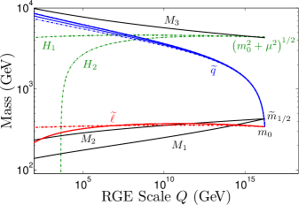
Figure 1: Two-loop renormalization group evolution of the soft parameters in ${}_{\widetilde{g}}\text{SUGRA}$. The input parameters used here are those of the best-fit point determined from our analysis in Section III. The fields are labeled in the figure and also in color. The gaugino fields are presented in black and the Higgs fields are presented in green. The squarks and sleptons are in blue and red, where the left-handed fields are solid and the right-handed fields are dot-dashed. Additionally, $m_{0}$ is the soft mass for the scalars, $\widetilde{m}_{1/2}$ is the common mass of the $\operatorname{U}(1)_{Y}$ and $\operatorname{SU}(2)_{L}$ gaugino fields, and $\mu$ is the Higgs mixing parameter.

The attractive feature of ${}_{\widetilde{g}}\text{SUGRA}$ is that the relatively large value of $M_{3}$ automatically drives the squarks to be massive while the sleptons as well as the bino and the light wino are left alone. This is illustrated in Fig. 1 where we display the renormalization group flow for a sample point from our analysis. We wish to show that this simple feature automatically satisfies all of the empirical results that we have discussed here that hint at the supersymmetric spectrum. To this end, we perform a Bayesian Monte Carlo analysis of ${}_{\widetilde{g}}\text{SUGRA}$ with the illustrative example of the $(1:1:10)$ gaugino mass ratio, which we discuss in the sections that follow.

Observable	Central value	Exp. Error	Th. Error	Distribution	Ref.
SM Nuisance Parameters
$m_{t}^{\mathrm{pole}}$ ($\mathrm{Ge\kern-0.80002ptV}$)	$173.5$	$1.0$	–	Gaussian	pdg2012
$m_{b}(m_{b})^{\overline{\mathrm{MS}}}$ ($\mathrm{Ge\kern-0.80002ptV}$)	$4.18$	$0.03$	–	Gaussian	pdg2012
$\alpha_{\mathrm{s}}(M_{Z})^{\overline{\mathrm{MS}}}$	0.1184	$7\times 10^{-4}$	–	Gaussian	pdg2012
$\alpha_{\mathrm{EM}}^{-1}(M_{Z})^{\overline{\mathrm{MS}}}$	$127.933$	0.014	–	Gaussian	pdg2012
Measured
$\delta a_{\mu}\times 10^{11}$	287	80	10	Gaussian	Bennett:2006fi ; Hagiwara:2011af ; Davier:2010nc
$\mathcal{B}r\left(B^{0}_{s}\to\mu^{+}\mu^{-}\right)\times 10^{9}$	3.2	1.92	14%	Gaussian	LHCb:2012nna
$\mathcal{B}r\left(B\to X_{s}\gamma\right)\times 10^{4}$	3.55	0.26	0.21	Gaussian	hfag2012
$\mathcal{B}r\left(B^{+}\to\tau^{+}\nu\right)\times 10^{4}$	1.79	0.48	0.38	Gaussian	hfag2012
$\omega_{\chi}$	0.1126	0.0036	10%	Upper-Gaussian	WMAP:2010fb
$h^{0}$ Mass ($\mathrm{Ge\kern-0.80002ptV}$)	$125.7$	$0.2$	$2.0$	Gaussian	CMS:2012nga ; ATLAS:2012oga
95% CL Particle Mass Limits ($\mathrm{Ge\kern-0.80002ptV}$)
$h^{0}$	$122.5$	–	–	Lower – Step Func.	CMS:2012tx
$h^{0}$	$129$	–	–	Upper – Step Func.	CMS:2012tx
$\widetilde{\chi}_{1}^{0}$	$46$	–	5%	Lower – Error Func.	pdg2012
$\widetilde{\chi}_{2}^{0}$	$62.4$	–	5%	Lower – Error Func.	pdg2012
$\widetilde{\chi}_{3}^{0}$	$99.9$	–	5%	Lower – Error Func.	pdg2012
$\widetilde{\chi}_{4}^{0}$	$116$	–	5%	Lower – Error Func.	pdg2012
$\widetilde{\chi}_{1}^{\pm}$	$94$	–	5%	Lower – Error Func.	pdg2012
$\widetilde{e}_{R}$	$107$	–	5%	Lower – Error Func.	pdg2012
$\widetilde{\mu}_{R}$	$94$	–	5%	Lower – Error Func.	pdg2012
$\widetilde{\tau}_{1}$	$81.9$	–	5%	Lower – Error Func.	pdg2012
$\widetilde{b}_{1}$	$89$	–	5%	Lower – Error Func.	pdg2012
$\widetilde{t}_{1}$	$95.7$	–	5%	Lower – Error Func.	pdg2012
$\widetilde{g}$	$500$	–	5%	Lower – Error Func.	pdg2012
$\widetilde{q}$	$1100$	–	5%	Lower – Error Func.	pdg2012

Table 1: Summary of the observables used to construct the likelihood function. The distribution labeled “Upper-Gaussian” used for the $\omega_{\chi}$ observable means that there is only a decrease in likelihood for values larger than the central value. The 95% CL limits are evaluated using the complementary error function, as the bound is smeared by the theoretical uncertainty. Limits specified with a step function distribution indicate a hard cut, where points on the wrong side of the limit are assigned zero likelihood.

III Statistical Framework

We study here the parameter space of ${}_{\widetilde{g}}\text{SUGRA}$ for the case where the ratio of the gaugino masses at the GUT scale is $1:1:10$. In this case, ${}_{\widetilde{g}}\text{SUGRA}$ is parametrized by $m_{0}$, $\widetilde{m}_{1/2}$, $A_{0}$, and $\tan\beta$ (having selected $\operatorname{sgn}\left(\mu\right)=1$). Here, $\widetilde{m}_{1/2}=M_{1}=M_{2}$ while $M_{3}=10\,\widetilde{m}_{1/2}$. The dimensionful parameters $m_{0}$, $\widetilde{m}_{1/2}$, and $A_{0}$ are all specified at the GUT scale. The ratio of the two Higgs VEVs $\tan\beta=\langle H_{2}\rangle/\langle H_{1}\rangle$, is specified at $M_{Z}$. We further include four Standard Model nuisance parameters to create an 8D parameter space. Namely, we add the top quark pole mass, the running bottom quark mass, the strong coupling, and the EM coupling. We create from these the parameter space $\mathbf{\Theta}$:

$$\begin{split}\mathbf{\Theta}=&\left\{m_{0},\widetilde{m}_{1/2},A_{0},\tan\beta,m_{t}^{\mathrm{pole}},\hskip 36.0pt\right.\\ &\hskip 24.0pt\left.m_{b}(m_{b})^{\overline{\mathrm{MS}}},\alpha_{\mathrm{s}}(M_{Z})^{\overline{\mathrm{MS}}},\alpha_{\mathrm{EM}}^{-1}(M_{Z})^{\overline{\mathrm{MS}}}\right\}~{}.\end{split}$$ (11)

For each parameter $\theta_{i}\in\mathbf{\Theta}$, we begin by selecting uniform distributions in the allowed ranges prior to considering the experimental data. The prior distributions that we have selected for our parameters are uniform on either a linear or a log scale:

$$\begin{split}m_{0}\in[50,5000]\,\mathrm{Ge\kern-0.80002ptV}\text{ (log)}\\ \widetilde{m}_{1/2}\in[50,2500]\,\mathrm{Ge\kern-0.80002ptV}\text{ (log)}\\ A_{0}\in[-50,50]\,\mathrm{Te\kern-0.80002ptV}\text{ (linear)}\\ \tan\beta\in[3,60]\text{ (linear)}~{}.\end{split}$$ (12)

The nuisance parameters in $\mathbf{\Theta}$ are uniform in a $2\,\sigma$ range (linear scale) around the central values, which are specified in Table 1.

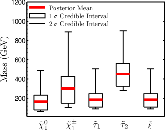
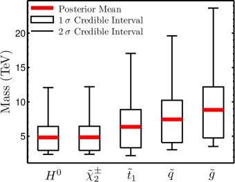
Figure 2: A display of the mass spectrum for sparticles and the Higgs boson with split scales, i.e., a low scale for $\tilde{\chi}_{1}^{0},\tilde{\chi}^{\pm}_{1},\tilde{\tau}_{1},\tilde{\tau}_{2},\tilde{\it l}$ and a high scale for $H^{0},\tilde{\chi}^{\pm}_{2},\tilde{t}_{1},\tilde{q},\tilde{g}$. Shown are the credible intervals in the superpartner masses from the Bayesian analysis of ${}_{\widetilde{g}}\text{SUGRA}$. The lighter superpartners are presented in the left panel, and the heavier are presented in the right panel. The posterior means are indicated in red.

Next we collect the relevant observables into $\mathbf{D}$, which is a set of pairs of central values and uncertainties of experimental measurements. The observables include the precise measurements of the nuisance parameters, along with the results from flavor physics $\mathcal{B}r\left(B^{0}_{s}\to\mu^{+}\mu^{-}\right)$ and $\mathcal{B}r\left(B\to X_{s}\gamma\right)$, the muon anomalous magnetic moment $\delta a_{\mu}$, the measured mass of the (ostensibly) light $CP$-even Higgs boson, as well as limits on superpartner masses. We further include the fit to the thermal relic density of dark matter, $\omega_{\chi}\equiv\Omega_{\chi}h^{2}$, from CMB temperature fluctuations measured by WMAP (9 year dataset) WMAP:2012fq and Planck (15.5 month dataset) Planck:2013xsa . In ${}_{\widetilde{g}}\text{SUGRA}$, the lightest neutralino is indeed a candidate for cold dark matter, but we wish to allow for multicomponent models of dark matter, and so we only consider the upper limit of $\omega_{\chi}$. The central values and uncertainties of $\mathbf{D}$ are specified in Table 1.

The goal now is to update our a priori guess for the probability distributions of the parameters in $\mathbf{\Theta}$ (given in Eq. 12) with the empirical information in $\mathbf{D}$, giving the posterior probability distribution. This distribution can then be marginalized to determine the credible region of one or two parameters. The calculation of the posterior probability distribution is achieved using Bayesian inference, but we first need to be able to compare a parametric point in our model to the empirical data in $\mathbf{D}$. This requires a set of mappings $\xi_{i}:\mathbf{\Theta}\to\mathbb{R}$ corresponding to each $d_{i}\in\mathbf{D}$, which just give the theoretical calculation for the observable corresponding to each $d_{i}$. These mappings are computed using numerical codes incorporated in our analysis software SusyKit susykit .

Now we can move on to constructing the posterior probability distribution, which is given by Bayes’ theorem

$$P(\mathbf{\Theta}|\mathbf{D})=\frac{P(\mathbf{D}|\mathbf{\Theta})P(\mathbf{\Theta})}{P(\mathbf{D})}~{}.$$ (13)

$P(\mathbf{\Theta})$ is the prior distribution given in Eq. 12. The denominator is the so-called Bayesian evidence $\mathcal{Z}=P(D)$, which can be used in model selection tests, but as we are only interested in parameter estimation, it serves as a normalization constant. The final factor is the likelihood function $\mathfrak{L}=P(\mathbf{D}|\mathbf{\Theta})$, which is constructed by the “pulls” method

$$-2\ln\mathfrak{L}=\sum\limits_{d_{i}\in\mathbf{D}}\frac{\left(\xi_{i}(\mathbf{\Theta})-d_{i}\right)^{2}}{\sigma_{i}^{2}+\tau_{i}^{2}}$$ (14)

where $\sigma_{i}$ and $\tau_{i}$ are the experimental and theoretical uncertainties, respectively. This is straightforward for the case that a measurement with precision is reported. In many cases only the 95% CL limits are given. In those cases, a smearing due to the implicit theoretical uncertainty in the computation is used and the likelihood is computed from the complementary error function. A hard cut on an observable can also be made by using a step function, i.e. assigning zero likelihood to points that are on the wrong side of a limit. The numerical values used to construct the likelihood function is given in Table 1.

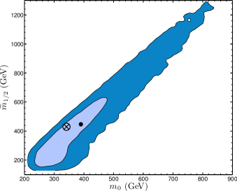
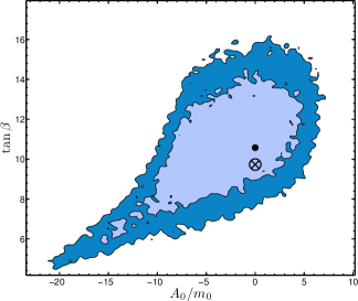
Figure 3: An exhibition of the $1\,\sigma$ and $2\,\sigma$ credible regions of the marginalized posterior probability distributions for the parameters of interest of ${}_{\widetilde{g}}\text{SUGRA}$. Left panel: the credible regions in $m_{0}$ and $\widetilde{m}_{1/2}$. Right panel: the credible regions in the dimensionless parameter $A_{0}/m_{0}$ and $\tan\beta$. The location of the best-fit point is indicated by a circled ‘X’ and the posterior mean is given with a solid dot.

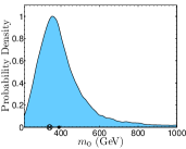
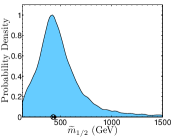
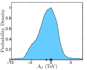
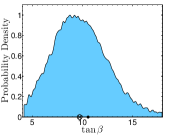
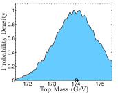
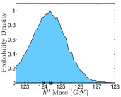
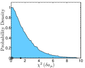
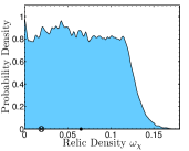
Figure 4: A display of the marginalized posterior probability distributions for ${}_{\widetilde{g}}\text{SUGRA}$ in the parameters of interest as well as some important derived quantities. The top row (left to right) gives the posterior PDF for $m_{0}$, $\widetilde{m}_{1/2}$, $A_{0}$, and $\tan\beta$, and the bottom row (left to right) displays the same for the top quark mass, the light $CP$ even Higgs boson mass, the contribution to $-2\ln\mathfrak{L}$ due to the anomalous magnetic moment of the muon (which we have denoted as $\chi^{2}(\delta a_{\mu})$, and the thermal relic density of cold dark matter, $\omega_{\chi}$. The location of the best-fit point is indicated by a circled ‘X’ and the posterior mean is given with a solid dot.

Our analysis was performed using our software package SusyKit susykit , which uses the efficient multi-modal ellipsoidal nested sampling algorithm implemented in the MultiNest Feroz:2007kg ; Feroz:2008xx ; Feroz:2011bj library. Additionally, SusyKit interfaces with several standard numerical codes such as SOFTSUSY Allanach:2001kg , MicrOMEGAs Belanger:2008sj ; Belanger:2010gh , FeynHiggs Heinemeyer:1998yj ; Hahn:2010te , and SuperIso Relic Mahmoudi:2009zz ; Arbey:2011zz . SusyKit is written entirely in C++11 and is largely inspired by the FORTRAN-90 code SuperBayes deAustri:2006pe ; superbayes .

We specify the MultiNest sampling parameters $n_{\mathrm{live}}=\text{5,000}$ and $\mathtt{tol}=0.01$. The analysis has required the evaluation of the likelihood function at 1.1 million points to sufficiently explore the parametric space. The result is a chain of 81,000 Monte Carlo sample points which is used to compute 1D and 2D marginalized distributions in our principal and derived parameters, and to establish credible regions in these parameters. We found that the credible regions entered areas that would be excluded by the LHC in minimal SUSY GUT models such as mSUGRA, so we found it necessary to evaluate the impact of LHC searches on ${}_{\widetilde{g}}\text{SUGRA}$.

IV LHC Analysis

In order to evaluate the impact of null results in the searches for supersymmetry at the LHC on ${}_{\widetilde{g}}\text{SUGRA}$, we construct an auxiliary likelihood function, $\mathfrak{L}_{\mathrm{LHC}}$, based on the Monte Carlo event generation and detector simulation for our sample points.

We begin by generating 200,000 events for each sample point in our chain using PYTHIA Sjostrand:2007gs ; Sjostrand:2006za considering $2\to 2$ SUSY production processes with $\mathchoice{{\hbox{$\displaystyle\sqrt{s\,}$}\lower 0.4pt\hbox{\vrule height=4.30554pt,depth=-3.44446pt}}}{{\hbox{$\textstyle\sqrt{s\,}$}\lower 0.4pt\hbox{\vrule height=4.30554pt,depth=-3.44446pt}}}{{\hbox{$\scriptstyle\sqrt{s\,}$}\lower 0.4pt\hbox{\vrule height=3.01389pt,depth=-2.41113pt}}}{{\hbox{$\scriptscriptstyle\sqrt{s\,}$}\lower 0.4pt\hbox{\vrule height=2.15277pt,depth=-1.72223pt}}}=8\,\mathrm{Te\kern-0.80002ptV}$. We find that the total cross section for these processes is $\mathcal{O}\left(100\,\mathrm{fb}\right)$ and the dominant modes involve the production of $\widetilde{\chi}_{1}^{0}$, $\widetilde{\chi}_{2}^{0}$, $\widetilde{\chi}_{1}^{\pm}$, $\tilde{\ell}$, $\widetilde{\tau}_{1}$, $\widetilde{\tau}_{2}$, and, $\tilde{\ell}$ and $\widetilde{\nu}$. This is to be expected because in ${}_{\widetilde{g}}\text{SUGRA}$, the scalar quark fields all become heavy as they are renormalized to the electroweak scale, while the scalar leptons are allowed to remain light to produce contributions to $\delta a_{\mu}$ and the Higgs diphoton decay rate. By investigating the dominant decays of these particles, we decide that supersymmetry searches in leptonic final states are the most relevant to ${}_{\widetilde{g}}\text{SUGRA}$. We have used the $3\ell$ and same-sign $2\ell$ searches at CMS CMS-PAS-SUS-12-022 using 9.2$\,\mathrm{fb}^{-1}$ at $\mathchoice{{\hbox{$\displaystyle\sqrt{s\,}$}\lower 0.4pt\hbox{\vrule height=4.30554pt,depth=-3.44446pt}}}{{\hbox{$\textstyle\sqrt{s\,}$}\lower 0.4pt\hbox{\vrule height=4.30554pt,depth=-3.44446pt}}}{{\hbox{$\scriptstyle\sqrt{s\,}$}\lower 0.4pt\hbox{\vrule height=3.01389pt,depth=-2.41113pt}}}{{\hbox{$\scriptscriptstyle\sqrt{s\,}$}\lower 0.4pt\hbox{\vrule height=2.15277pt,depth=-1.72223pt}}}=8\,\mathrm{Te\kern-0.80002ptV}$ to construct our $\mathfrak{L}_{\mathrm{LHC}}$. These searches are performed using 108 and 4 event bins respectively, which serve as counting experiments and are naturally Poisson distributed. Therefore $\mathfrak{L}_{\mathrm{LHC}}$ is computed by

$$\mathfrak{L}_{\mathrm{LHC}}=\prod\limits_{i\in\mathrm{bins}}\mathfrak{L}_{i}~{}.$$ (15)

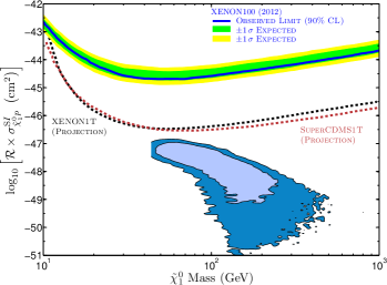
Figure 5: A display of the $1\,\sigma$ and $2\,\sigma$ credible regions of the marginalized posterior PDF of ${}_{\widetilde{g}}\text{SUGRA}$ in the plane of the spin-independent $p$–$\widetilde{\chi}_{1}^{0}$ cross section and the $\widetilde{\chi}_{1}^{0}$ mass. The current limit from XENON100 is displayed as well as the projected sensitivities for XENON1T and SuperCDMS1T.

Each $\mathfrak{L}_{i}$ would be a simple Poisson likelihood, except that one of the parameters to the Poisson distribution, the expected background yield, $b_{i}$, can have a large uncertainty, $\delta b_{i}$. Thus, it is necessary to convolve the Poisson distribution with a distribution for the background yield. Naïvely this would be a Gaussian distribution, however in the case that the relative error in the background yield is large, i.e., $\delta b_{i}/b_{i}\gtrsim 20\%$, then a non-trivial portion of the convolution is due to contributions from negative $b_{i}$, or even if the integration is limited to non-negative background, a large portion of the PDF may be omitted. Thus as a heuristic, we use the following definition for $\mathfrak{L}_{i}$:

$$\mathfrak{L}_{i}=\int_{0}^{\infty}\operatorname{Pois}(s_{i}+\bar{b};o_{i})F(b_{i},\delta b_{i};\bar{b})~{},$$ (16)

where $i$ is the event bin, $\operatorname{Pois}$ is the Poisson probability mass function, $s_{i}$ is the expected signal yield, $o_{i}$ is the number of observed events, and as defined already $b_{i}$ is the expected background yield, and $\delta b_{i}$ is the uncertainty in the background. The function F is defined according to our heuristic

$$F(b_{i},\delta b_{i};\bar{b})=\begin{cases}\mathcal{N}(b_{i},\delta b_{i};\bar{b})\text{ , $\delta b_{i}/b_{i}<20\%$}\\ \ln\mathcal{N}(b_{i},\delta b_{i};\bar{b})\text{ , $\delta b_{i}/b_{i}\geq 20\%$}\end{cases}~{},$$ (17)

where $\mathcal{N}$ is the Gaussian distribution and $\ln\mathcal{N}$ is the log-normal distribution. As a further heuristic, it is necessary to account for cases when either $b_{i}=0$ or $\delta b_{i}=0$. These cases are clearly oversights in the CMS preliminary analysis summary; still they must be addressed. We choose a sentinel value $\Delta=10^{-6}$ and use $\delta b_{i}=\Delta$ if $\delta b_{i}$ is zero and we set $b_{i}=\delta b_{i}$ if $b_{i}$ is zero.

The expected signal yield $s_{i}$ is the product of the efficiency $\epsilon_{i}$ with the total SUSY cross section and the integrated luminosity. The efficiency $\epsilon_{i}$ is the proportion of the total generated events that would be counted in the $i^{\mathrm{th}}$ bin, and is determined by running the events through a detector simulation, which we have carried out with PGS4 Conway:PGS . Jet objects were reconstructed using the anti-$k_{\mathrm{T}}$ algorithm, with a distance parameter of 0.5. We implemented the cuts to place events into bins in a modified version of Parvicursor parvicursor . The object selection criteria, event vetoes, and geometrical cuts are reproduced as in CMS-PAS-SUS-12-022 .

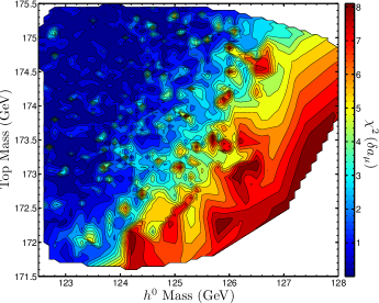
Figure 6: A display of level curves in the statistic $\chi^{2}\left(\delta a_{\mu}\right)$, which is the contribution to $-2\ln\mathfrak{L}$ due to $\delta a_{\mu}$. The level curves are given in the plane of the top mass and $h^{0}$ mass. The level curves are constructed by interpolating equally-weighted sample points.

To combine the likelihood from these searches to the likelihood function described in Section III, we first compute the likelihood for the Standard Model according to this analysis by turning off the signal, $\mathfrak{L}_{\mathrm{SM}}=\left.\mathfrak{L}_{\mathrm{LHC}}\right|_{s=0}$. We then add the likelihood ratio statistic to the full likelihood function,

$$-2\ln\mathfrak{L}\to-2\ln\mathfrak{L}-2\ln{\left(\min\left\{\frac{\mathfrak{L_{\mathrm{LHC}}}}{\mathfrak{L_{\mathrm{SM}}}},1\right\}\right)}~{},$$ (18)

which is approximately $\chi^{2}$ distributed, and is a natural addition to the other “pull” terms in our likelihood function. Having computed the updated likelihood due to these CMS searches, it is necessary to re-weight the samples by a factor $\exp\left(\Delta\ln\mathfrak{L}\right)$. We can now proceed to determine the marginalized posterior probability distributions within our parameters of interest.

V Results

In this section we present the results from our Bayesian analysis. Given our likelihood function, we determine the Bayesian evidence of ${}_{\widetilde{g}}\text{SUGRA}$ to be $\ln\mathcal{Z}=-11.9\pm 0.042$. We provide this for reference, as we do not perform a model selection test. The best-fit point in our analysis is determined to have $\chi^{2}_{\mathrm{min}}=2.73$, and leaving out some of the nuisance parameters, is specified by $(m_{0},\widetilde{m}_{1/2},A_{0},\tan\beta,m_{t}^{\mathrm{pole}})=(341,429,298,9.73,174)$ where the massive parameters are specified in $\mathrm{Ge\kern-0.80002ptV}$. This point illustrates the general result of ${}_{\widetilde{g}}\text{SUGRA}$ that high $h^{0}$ mass and $\delta a_{\mu}$ can be simultaneously satisfied. Additionally, the large scalar quark and gluino masses allow for consistency with $\mathcal{B}r\left(B^{0}_{s}\to\mu^{+}\mu^{-}\right)$ and $\mathcal{B}r\left(B\to X_{s}\gamma\right)$. The credible regions in the masses of the heavier particles in ${}_{\widetilde{g}}\text{SUGRA}$ are presented in the right panel of Fig. 2, and the light particles of ${}_{\widetilde{g}}\text{SUGRA}$ that create the $\delta a_{\mu}$ contribution as well as the contribution to the diphoton Higgs decay are given in the left panel.

The $1\,\sigma$ and $2\,\sigma$ credible regions in our parameters of interest are given in Fig. 3, where we have chosen to use the dimensionless parameter $A_{0}/m_{0}$. The 1D posterior distributions in these parameters are given in the top panels of Fig. 4, though here we did give the distribution for the dimensionful parameter $A_{0}$.

While ${}_{\widetilde{g}}\text{SUGRA}$ largely achieves the correct $h^{0}$ mass and $\delta a_{\mu}$ contribution as shown in the middle two lower panels of Fig. 4, the posterior distribution in the top mass is shifted up from the central value by 0.5$\,\mathrm{Ge\kern-0.80002ptV}$ to 174$\,\mathrm{Ge\kern-0.80002ptV}$, which is evident in the lower left panel of Fig. 4. The tension between the top mass, the $h^{0}$ mass and $\delta a_{\mu}$ is clearly displayed in Fig. 6 where we have interpolated sample points from a slice in our likelihood function and presented level curves in “$\chi^{2}(\delta a_{\mu})$” which is the contribution to $-2\ln\mathfrak{L}$ due to $\delta a_{\mu}$. It is evident that the higher $h^{0}$ mass and $\delta a_{\mu}$ is best matched in ${}_{\widetilde{g}}\text{SUGRA}$ for a slightly heavier top quark.

We point out that this tension is not overly significant in ${}_{\widetilde{g}}\text{SUGRA}$ for two reasons. First, there is a large theoretical uncertainty in the calculation of the $h^{0}$ mass at the 2-loop level, which when considered does lift most of the tension. Next, we specified in ${}_{\widetilde{g}}\text{SUGRA}$ $M_{3}=10\,\widetilde{m}_{1/2}$, where 10 is an arbitrary choice. Allowing the coefficient to be a new degree of freedom or simply selecting several different choices will likely resolve this tension as well.

In our Bayesian analysis, we have sampled the parameter space using the older WMAP7 value for $\omega_{\chi}$ in $\mathcal{L}$ but we can see from the fourth panel from the left in the bottom row of Fig. 4 that the slightly larger value indicated by WMAP9 and Planck would simply enlarge our credible region. Additionally, we see in Fig. 5 that ${}_{\widetilde{g}}\text{SUGRA}$ is not currently constrained by the best available limit on the direct detection of $\widetilde{\chi}_{1}^{0}$ dark matter, and is slightly beyond the projected sensitivity of XENON1T and SuperCDMS1T, creating a sort of nightmare scenario for dark matter experiments, as our dark matter signal would be competing with the cosmic neutrino background. The LSP in our model is consistently a bino, and the $\widetilde{\chi}_{2}^{0}$ is a wino. There is virtually no mixing with the Higgsino sector as the Higgsino mass parameter $\mu$ becomes very large due to the large $M_{3}$. The sensitivity to dark matter experiments can be increased by adjusting the ratio of $M_{1}$ to $M_{2}$ to allow for greater bino-wino mixing within the LSP state.

One of the exceptional aspects of ${}_{\widetilde{g}}\text{SUGRA}$ is the presence of many light superpartners that have thus far evaded detection at the LHC. We concede that the searches that we considered here are not by any means comprehensive, but they are designed to constrain the production modes most prevalent in ${}_{\widetilde{g}}\text{SUGRA}$. The limits are evaded largely due to the stringent selection criteria and the difficulty in identifying $\tau$ leptons. Additionally, the mass hierarchy of ${}_{\widetilde{g}}\text{SUGRA}$ limits the possibility of cascading decays.

We note that the parametric space of ${}_{\widetilde{g}}\text{SUGRA}$, naturally fits into the Hyperbolic Branch Chan:1997bi ; Chattopadhyay:2003xi ; Baer:2003wx of radiative breaking of the electroweak symmetry. This is due to the fact that the stop masses are driven to be large by the gluino, giving a large $Q=\mathchoice{{\hbox{$\displaystyle\sqrt{m_{\widetilde{t}_{1}}m_{\widetilde{t}_{2}}\,}$}\lower 0.4pt\hbox{\vrule height=4.30554pt,depth=-3.44446pt}}}{{\hbox{$\textstyle\sqrt{m_{\widetilde{t}_{1}}m_{\widetilde{t}_{2}}\,}$}\lower 0.4pt\hbox{\vrule height=4.30554pt,depth=-3.44446pt}}}{{\hbox{$\scriptstyle\sqrt{m_{\widetilde{t}_{1}}m_{\widetilde{t}_{2}}\,}$}\lower 0.4pt\hbox{\vrule height=3.01389pt,depth=-2.41113pt}}}{{\hbox{$\scriptscriptstyle\sqrt{m_{\widetilde{t}_{1}}m_{\widetilde{t}_{2}}\,}$}\lower 0.4pt\hbox{\vrule height=2.15277pt,depth=-1.72223pt}}}$, and it was shown in Akula:2011jx ; Liu:2013ula that $Q\gtrsim 1\,\mathrm{Te\kern-0.80002ptV}$ corresponds to a hyperbolic geometry of soft parameters that give radiative EWSB (a large SUSY scale in the tens of TeV also arises in a certain class of string motivated models Acharya:2008zi ; Feldman:2011ud ). Still, ${}_{\widetilde{g}}\text{SUGRA}$ as it stands produces a large value of $\mu$ with respect to the $Z$ mass. Specifically, a large value of $\mu$ is necessary to balance the large value of $M_{3}$ which enters in the corrections to the $H_{2}$ field mass.

V.1 Higgs Diphoton Decay

In the Standard Model, the loop-induced decay of the Higgs into two photons is mediated mainly by the $W$, top, and to a lesser extent, the bottom quark. The partial width reads Djouadi:2005gi

$$\Gamma\left(H\to\gamma\gamma\right)=\frac{\alpha^{2}_{\mathrm{EM}}m_{H}^{2}}{256v^{2}\pi^{3}}\left\lvert\sum\limits_{f=t,b}N_{c,f}Q_{f}^{2}A_{1/2}(\tau_{f})+A_{1}(\tau_{W})\right\rvert^{2}$$ (19)

where $\tau_{i}$ = $4m_{i}^{2}/m_{H}^{2}$, and the spin form factors are

$$A_{1/2}(\tau)=2\tau\left(1-(\tau-1)f(\tau)\right)$$ (20)

$$A_{1}(\tau)=-\left(2+3\tau-3\tau(\tau-2)f(\tau)\right)$$ (21)

and the universal scaling function $f(\tau)$ is

$$f(\tau)=\begin{cases}\begin{array}[]{lr}\arcsin^{2}\left(\tau^{-1/2}\right)&:\tau\geq 1\\ -\dfrac{1}{4}\left(\ln\dfrac{1+\mathchoice{{\hbox{$\displaystyle\sqrt{1-\tau\,}$}\lower 0.4pt\hbox{\vrule height=6.44444pt,depth=-5.15558pt}}}{{\hbox{$\textstyle\sqrt{1-\tau\,}$}\lower 0.4pt\hbox{\vrule height=6.44444pt,depth=-5.15558pt}}}{{\hbox{$\scriptstyle\sqrt{1-\tau\,}$}\lower 0.4pt\hbox{\vrule height=4.51111pt,depth=-3.6089pt}}}{{\hbox{$\scriptscriptstyle\sqrt{1-\tau\,}$}\lower 0.4pt\hbox{\vrule height=3.22221pt,depth=-2.57779pt}}}}{1-\mathchoice{{\hbox{$\displaystyle\sqrt{1-\tau\,}$}\lower 0.4pt\hbox{\vrule height=6.44444pt,depth=-5.15558pt}}}{{\hbox{$\textstyle\sqrt{1-\tau\,}$}\lower 0.4pt\hbox{\vrule height=6.44444pt,depth=-5.15558pt}}}{{\hbox{$\scriptstyle\sqrt{1-\tau\,}$}\lower 0.4pt\hbox{\vrule height=4.51111pt,depth=-3.6089pt}}}{{\hbox{$\scriptscriptstyle\sqrt{1-\tau\,}$}\lower 0.4pt\hbox{\vrule height=3.22221pt,depth=-2.57779pt}}}}-\imath\pi\right)^{2}&:\tau<1\end{array}\end{cases}~{}.$$ (22)

Supersymmetry corrects this partial width Djouadi:2005gj by factors involving the Higgs mixing angle $\alpha$ and $\beta$ arising from the two Higgs doublets. Additionally, new amplitudes are available mediated by the charged Higgs, charginos, and sfermions. The couplings to the charginos arise from Higgsino–gaugino mixing, but in ${}_{\widetilde{g}}\text{SUGRA}$ the Higgsinos are very heavy thus the lighter chargino is always purely charged wino while the heavier one is purely charged Higgsino. This means that overall the chargino contribution is small either because the coupling is suppressed or because the mass is too large. The charged Higgs exchange is also suppressed due to its large mass. Thus the largest contributions can come only from the sfermion sector, which in ${}_{\widetilde{g}}\text{SUGRA}$ is dominated by the staus.

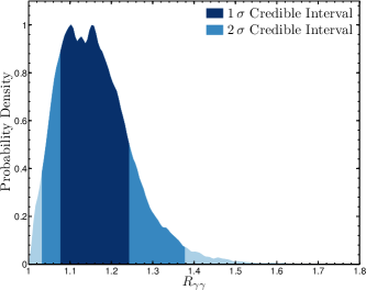
Figure 7: A display of the marginalized posterior probability density of $R_{\gamma\gamma}$ from our analysis. The $1\,\sigma$ and $2\,\sigma$ credible intervals are indicated in darker blues. We define $R_{\gamma\gamma}$ as the ratio of the diphoton partial width of the light $CP$-even Higgs boson to the corresponding width for a Standard Model Higgs of the same mass (see Eq. 8).

In the decoupling limit where $M_{A}\gg M_{Z}$ which corresponds to $\alpha=\beta-\pi/2$, the Higgs coupling to the staus is given by Giudice:2012pf ; Feng:2013mea

$$g_{h^{0}\widetilde{\tau}_{i}\widetilde{\tau}_{i}}=I_{3}^{\tau}c_{i}\mp Q_{\tau}\sin^{2}\theta_{\mathrm{W}}\cos{2\theta_{\widetilde{\tau}}}\\ \mp\frac{m_{\tau}(A_{\ell}-\mu\tan\beta)}{2M_{Z}^{2}}\sin{2\theta_{\widetilde{\tau}}}-\frac{m_{\tau}^{2}}{M_{Z}^{2}}$$ (23)

with $c_{1}=\cos^{2}{\theta_{\widetilde{\tau}}}$, and $c_{2}=\sin^{2}{\theta_{\widetilde{\tau}}}$. The ‘$-$’ case corresponds to $i=1$, and the ‘$+$’ case corresponds to $i=2$. The partial width in ${}_{\widetilde{g}}\text{SUGRA}$ including the amplitude due to staus then reads

$$\Gamma\left(h^{0}\to\gamma\gamma\right)=\frac{\alpha^{2}_{\mathrm{EM}}m_{H}^{2}}{256v^{2}\pi^{3}}\left\lvert\sum\limits_{f=t,b}N_{c,f}Q_{f}^{2}A_{1/2}(\tau_{f})\right.\\ \left.+A_{1}(\tau_{W})+\sum\limits_{i=1,2}g_{h^{0}\widetilde{\tau}_{1}\widetilde{\tau}_{2}}\frac{M_{Z}^{2}}{m_{\widetilde{\tau}}^{2}}A_{0}(\tau_{i})\right\rvert^{2}$$ (24)

and the spin zero form factor is

$$A_{0}(\tau)=-\tau(1-\tau f(\tau))~{}.$$ (25)

We identify the ratio of this partial width to the Standard Model width given in Eq. 19 as $R_{\gamma\gamma}$. (We have taken the ratio of the theoretical and observed $h^{0}$ production to be unity.) We compute this ratio for each of our Monte Carlo samples and construct the 1D posterior PDF in this derived parameter which we present in Fig. 7. We find that ${}_{\widetilde{g}}\text{SUGRA}$ generically produces a $\sim 20\%$ boost to this decay mode over the Standard Model case. The $2\,\sigma$ credible interval is $[1.03,1.38]$, which is quite consistent with the preliminary results arriving from the LHC.

VI Conclusion

The recent observation of the Higgs boson mass around 125$\,\mathrm{Ge\kern-0.80002ptV}$ points to large loop corrections which can be achieved with a large weak scale of SUSY. A large SUSY scale also explains the suppression of SUSY contributions to the decay $B^{0}_{s}\to\mu^{+}\mu^{-}$, to be consistent with the recently measured branching ratio for this process. On the other hand, the experimental observation of a $3\sigma$ effect in $\delta a_{\mu}$ and a possible excess in the diphoton rate $R_{\gamma\gamma}$ in the Higgs boson decay over the standard model prediction cannot be explained with a high SUSY scale. Thus the two sets of data point to a two scale SUSY spectrum, one a high scale consisting of colored particles, i.e., the squarks and the gluinos, and the Higgs bosons (aside from the lightest Higgs) and the other a low scale for masses of uncolored particles including sleptons and the electroweak gauginos.

In this work we discuss the high scale supergravity grand unified model, ${}_{\widetilde{g}}\text{SUGRA}$, which includes the feature of a two scale sparticle spectrum where the sparticle spectrum is widely split at the electroweak scale. This is accomplished within supergravity grand unification with non-universal gaugino masses such that $M_{3}\gg M_{1},M_{2},m_{0}$. As an illustration we consider the specific case where $M_{1}:M_{2}:M_{3}=1:1:10$ at the unification scale, $M_{1}=M_{2}=\tilde{m}_{1/2}$ and $M_{3}>>m_{0}$. This case is designed to be mainly illustrative and can be easily embedded within $\operatorname{SU}(5)$ and $\operatorname{SO}(10)$. Using a Bayesian Monte Carlo analysis, It is found that this construction simultaneously explains the high $h^{0}$ mass, null results for squarks and gluino searches at the LHC, a negligible correction to the branching ratio for $B^{0}_{s}\to\mu^{+}\mu^{-}$, a $3\sigma$ deviation of $g_{\mu}-2$ from the Standard Model prediction as well as the nascent excess in the diphoton signal of the Higgs.

The observable sparticle spectrum at the LHC in this model consists of light sleptons and light electroweak gauginos. However, sleptons and electroweak gauginos are typically difficult to observer at the LHC and thus far have evaded detection in multi-lepton searches in experiments at the ATLAS and the CMS detectors with the 7 $\,\mathrm{Te\kern-0.80002ptV}$ and 8 $\,\mathrm{Te\kern-0.80002ptV}$ data. The most promising $2\to 2$ processes that can generate sparticles at the LHC in this model are $pp\to\widetilde{\chi}_{1}^{\pm}\widetilde{\chi}_{1}^{\mp},\widetilde{\chi}_{2}^{0}\widetilde{\chi}_{1}^{\pm}$. The identifying signatures of such processes will indeed be multi-leptons and missing energy. It is hoped that at increased energies and with larger luminosities such signals will lie in the observable region. However, a detailed analysis of the signals in needed requiring a knowledge of the backgrounds for these processes.

Another aspect of the simplified ${}_{\widetilde{g}}\text{SUGRA}$ model relates to the spin-independent $\tilde{\chi}_{1}^{0}-p$ cross section. This cross section is found to be rather small for the case when the gaugino masses are chosen in the ratio $(1:1:10)$. The reason for this smallness is easily understood. The constraint $M_{1}=M_{2}$ at the GUT scale, leads to an LSP which is essentially purely bino with very little Higgsino or wino content. The purely bino nature of the LSP leads to a suppressed $\tilde{\chi}_{1}^{0}-p$ cross section (see e.g., Feldman:2010ke ) which lies beyond the reach of the current and projected sensitivities for direct-detection experiments. However, the above result is very specific to the $M_{1}:M_{2}:M_{3}=1:1:10$ assumption and a modification of the above should allow $\tilde{\chi}_{1}^{0}-p$ cross section within the observable range in the projected sensitivities for direct-detection experiments. We note that while our analysis was performed using the older WMAP7 measurement of the cold dark matter relic density, the newer measurements from WMAP9 and Planck (with 15.5 months of data) only slightly increase the measurement. As we only apply the upper limit from these measurements to allow for the possibility of multi-component theories of dark matter, the newer results would only expand the credible regions of our parameter space and either increase or not affect at all the likelihood of our best-fit point.

Finally, we note that the large squark masses in ${}_{\widetilde{g}}\text{SUGRA}$ would also help stabilize the proton against decay from baryon and lepton number violating dimension five operators Arnowitt:1993pd ; Liu:2013ula ; Hisano:2013exa (for a review see Nath:2006ut ).

- (1) CMS Collaboration, Phys. Lett. B 716 (2012) 30–61, arXiv:1207.7235.
- (2) ATLAS Collaboration, Phys. Lett. B 716 (2012) 1–29, arXiv:1207.7214.
- (3) CMS Collaboration, Science 338 (2012) 1569–1575.
- (4) ATLAS Collaboration, Science 338 (2012) 1576–1582.
- (5) CMS Collaboration, arXiv:1303.4571.
- (6) F. Englert and R. Brout, Phys. Rev. Lett. 13 (1964) 321–323.
- (7) P. W. Higgs, Phys. Lett. 12 (1964) 132–133.
- (8) P. W. Higgs, Phys. Rev. Lett. 13 (1964) 508–509.
- (9) G. Guralnik, C. Hagen, and T. Kibble, Phys. Rev. Lett. 13 (1964) 585–587.
- (10) S. Akula, B. Altunkaynak, D. Feldman et al., Phys. Rev. D 85 (2012) 075001, arXiv:1112.3645.
- (11) H. Baer, V. Barger, and A. Mustafayev, Phys. Rev. D 85 (2012) 075010, arXiv:1112.3017.
- (12) A. Arbey, M. Battaglia, A. Djouadi et al., Phys. Lett. B 708 (2012) 162–169, arXiv:1112.3028.
- (13) P. Draper, P. Meade, M. Reece et al., Phys. Rev. D 85 (2012) 095007, arXiv:1112.3068.
- (14) M. ”Carena, S. Gori, N. R. Shah et al., JHEP 1203 (2012) 014, arXiv:1112.3336.
- (15) S. Akula, P. Nath, and G. Peim, Phys. Lett. B 717 (2012) 188–192, arXiv:1207.1839.
- (16) C. Strege, G. Bertone, F. Feroz et al., arXiv:1212.2636.
- (17) A. H. Chamseddine, R. L. Arnowitt, and P. Nath, Phys. Rev. Lett. 49 (1982) 970.
- (18) P. Nath, R. L. Arnowitt, and A. H. Chamseddine, Nucl. Phys. B 227 (1983) 121.
- (19) L. J. Hall, J. D. Lykken, and S. Weinberg, Phys. Rev. D 27 (1983) 2359–2378.
- (20) R. L. Arnowitt and P. Nath, Phys. Rev. Lett. 69 (1992) 725–728.
- (21) A. Arbey, M. Battaglia, A. Djouadi et al., arXiv:1207.1348.
- (22) J. Ellis and K. A. Olive, Eur. Phys. J. C 72 (2012) 2005, arXiv:1202.3262.
- (23) O. Buchmueller, R. Cavanaugh, A. De Roeck et al., Eur. Phys. J. C 72 (2012) 2020, arXiv:1112.3564.
- (24) H. Baer, V. Barger, P. Huang et al., arXiv:1210.3019.
- (25) P. Nath, arXiv:1210.0520.
- (26) P. Nath, R. L. Arnowitt, and A. H. Chamseddine, “Applied Supergravity”, volume 1 of ICTP Series in Theoretical Physics. World Scientific, Singapore, 1984.
- (27) M. S. Carena and H. E. Haber, Prog. Part. Nucl. Phys. 50 (2003) 63–152, arXiv:hep-ph/0208209.
- (28) A. Djouadi, Phys. Rept. 459 (2008) 1–241, arXiv:hep-ph/0503173.
- (29) “LHC Performance and Statistics”, https://lhc-statistics.web.cern.ch/LHC-Statistics/.
- (30) LHCb Collaboration, Phys. Rev. Lett. 110 (2013) 021801, arXiv:1211.2674.
- (31) S. R. Choudhury and N. Gaur, Phys. Lett. B 451 (1999) 86–92, arXiv:hep-ph/9810307.
- (32) K. Babu and C. F. Kolda, Phys. Rev. Lett. 84 (2000) 228–231, arXiv:hep-ph/9909476.
- (33) C. Bobeth, T. Ewerth, F. Kruger et al., Phys. Rev. D 64 (2001) 074014, arXiv:hep-ph/0104284.
- (34) T. Ibrahim and P. Nath, Phys. Rev. D 67 (2003) 016005, arXiv:hep-ph/0208142.
- (35) T. Ibrahim and P. Nath, Rev. Mod. Phys. 80 (2008) 577–631, arXiv:0705.2008.
- (36) G. Degrassi, P. Gambino, and P. Slavich, Phys. Lett. B 635 (2006) 335–342, arXiv:hep-ph/0601135.
- (37) S. Akula, D. Feldman, P. Nath et al., Phys. Rev. D 84 (2011) 115011, arXiv:1107.3535.
- (38) S. Bertolini, F. Borzumati, A. Masiero et al., Nucl. Phys. B 353 (1991) 591–649.
- (39) Muon G-2 Collaboration, Phys. Rev. D 73 (2006) 072003, arXiv:hep-ex/0602035.
- (40) K. Hagiwara, R. Liao, A. D. Martin et al., J. Phys. G 38 (2011) 085003, arXiv:1105.3149.
- (41) M. Davier, A. Hoecker, B. Malaescu et al., Eur. Phys. J. C 71 (2011) 1515, arXiv:1010.4180.
- (42) T. Yuan, R. L. Arnowitt, A. H. Chamseddine et al., Z. Phys. C 26 (1984) 407.
- (43) D. A. Kosower, L. M. Krauss, and N. Sakai, Phys. Lett. B 133 (1983) 305.
- (44) J. L. Lopez, D. V. Nanopoulos, and X. Wang, Phys. Rev. D 49 (1994) 366–372, arXiv:hep-ph/9308336.
- (45) U. Chattopadhyay and P. Nath, Phys. Rev. D 53 (1996) 1648–1657, arXiv:hep-ph/9507386.
- (46) T. Moroi, Phys. Rev. D 53 (1996) 6565–6575, arXiv:hep-ph/9512396.
- (47) T. Ibrahim and P. Nath, Phys. Rev. D 62 (2000) 015004, arXiv:hep-ph/9908443.
- (48) S. Heinemeyer, D. Stockinger, and G. Weiglein, Nucl. Phys. B 690 (2004) 62–80, arXiv:hep-ph/0312264.
- (49) A. Sirlin and A. Ferroglia, arXiv:1210.5296.
- (50) J. Baglio, A. Djouadi, and R. Godbole, Phys. Lett. B 716 (2012) 203–207, arXiv:1207.1451.
- (51) G. F. Giudice, P. Paradisi, A. Strumia et al., JHEP 1210 (2012) 186, arXiv:1207.6393.
- (52) W.-Z. Feng and P. Nath, arXiv:1303.0289.
- (53) K. Inoue, A. Kakuto, H. Komatsu et al., Prog. Theor. Phys. 68 (1982) 927.
- (54) L. E. Ibanez and G. G. Ross, Phys. Lett. B 110 (1982) 215–220.
- (55) L. Alvarez-Gaume, J. Polchinski, and M. B. Wise, Nucl. Phys. B 221 (1983) 495.
- (56) L. Ibanez and G. Ross, Comptes Rendus Physique 8 (2007) 1013–1028, arXiv:hep-ph/0702046.
- (57) J. R. Ellis, K. Enqvist, D. V. Nanopoulos et al., Phys. Lett. B 155 (1985) 381.
- (58) M. Drees, Phys. Lett. B 158 (1985) 409.
- (59) P. Nath and R. L. Arnowitt, Phys. Rev. D 56 (1997) 2820–2832, arXiv:hep-ph/9701301.
- (60) J. R. Ellis, K. A. Olive, and Y. Santoso, Phys. Lett. B 539 (2002) 107–118, arXiv:hep-ph/0204192.
- (61) G. Anderson, H. Baer, C.-h. Chen et al., Phys. Rev. D 61 (2000) 095005, arXiv:hep-ph/9903370.
- (62) K. Huitu, Y. Kawamura, T. Kobayashi et al., Phys. Rev. D 61 (2000) 035001, arXiv:hep-ph/9903528.
- (63) A. Corsetti and P. Nath, Phys. Rev. D 64 (2001) 125010, arXiv:hep-ph/0003186.
- (64) U. Chattopadhyay and P. Nath, Phys. Rev. D 65 (2002) 075009, arXiv:hep-ph/0110341.
- (65) U. Chattopadhyay, A. Corsetti, and P. Nath, Phys. Rev. D 66 (2002) 035003, arXiv:hep-ph/0201001.
- (66) S. P. Martin, Phys. Rev. D 79 (2009) 095019, arXiv:0903.3568.
- (67) D. Feldman, Z. Liu, and P. Nath, Phys. Rev. D 80 (2009) 015007, arXiv:0905.1148.
- (68) I. Gogoladze, F. Nasir, and Q. Shafi, arXiv:1212.2593.
- (69) M. A. Ajaib, I. Gogoladze, Q. Shafi et al., arXiv:1303.6964.
- (70) P. Nath, B. D. Nelson, H. Davoudiasl et al., Nucl. Phys. Proc. Suppl. 200-202 (2010) 185–417, arXiv:1001.2693.
- (71) N. Arkani-Hamed and S. Dimopoulos, JHEP 0506 (2005) 073, arXiv:hep-th/0405159.
- (72) B. L. Kaufman, B. D. Nelson, and M. K. Gaillard, arXiv:1303.6575.
- (73) M. Ibe, T. T. Yanagida, and N. Yokozaki, arXiv:1303.6995.
- (74) S. Mohanty, S. Rao, and D. Roy, arXiv:1303.5830.
- (75) G. Bhattacharyya, B. Bhattacherjee, T. T. Yanagida et al., arXiv:1304.2508.
- (76) Particle Data Group, Phys. Rev. D 86 (2012) 010001.
- (77) Heavy Flavor Averaging Group, arXiv:1207.1158.
- (78) WMAP Collaboration, Astrophys. J. Suppl. 192 (2011) 18, arXiv:1001.4538.
- (79) CMS Collaboration, Phys. Lett. B 710 (2012) 26–48, arXiv:1202.1488.
- (80) WMAP Collaboration, arXiv:1212.5226.
- (81) Planck Collaboration, arXiv:1303.5062.
- (82) S. Akula, “SusyKit”, http://freeboson.org/software/.
- (83) F. Feroz and M. Hobson, Mon. Not. Roy. Astron. Soc. 384 (2008) 449, arXiv:0704.3704.
- (84) F. Feroz, M. Hobson, and M. Bridges, Mon. Not. Roy. Astron. Soc. 398 (2009) 1601–1614, arXiv:0809.3437.
- (85) F. Feroz, K. Cranmer, M. Hobson et al., JHEP 1106 (2011) 042, arXiv:1101.3296.
- (86) B. Allanach, Comput. Phys. Commun. 143 (2002) 305–331, arXiv:hep-ph/0104145.
- (87) G. Belanger, F. Boudjema, A. Pukhov et al., Comput. Phys. Commun. 180 (2009) 747–767, arXiv:0803.2360.
- (88) G. Belanger, F. Boudjema, P. Brun et al., Comput. Phys. Commun. 182 (2011) 842–856, arXiv:1004.1092.
- (89) S. Heinemeyer, W. Hollik, and G. Weiglein, Comput. Phys. Commun. 124 (2000) 76–89, arXiv:hep-ph/9812320.
- (90) T. Hahn, S. Heinemeyer, W. Hollik et al., Nucl. Phys. Proc. Suppl. 205-206 (2010) 152–157, arXiv:1007.0956.
- (91) F. Mahmoudi, Comput. Phys. Commun. 180 (2009) 1718–1719.
- (92) A. Arbey and F. Mahmoudi, Comput. Phys. Commun. 182 (2011) 1582–1583.
- (93) R. R. de Austri, R. Trotta, and L. Roszkowski, JHEP 0605 (2006) 002, arXiv:hep-ph/0602028.
- (94) R. R. de Austri, R. Trotta, and F. Feroz, “SuperBayes”, http://superbayes.org/.
- (95) T. Sjostrand, S. Mrenna, and P. Z. Skands, Comput. Phys. Commun. 178 (2008) 852–867, arXiv:0710.3820.
- (96) T. Sjostrand, S. Mrenna, and P. Z. Skands, JHEP 0605 (2006) 026, arXiv:hep-ph/0603175.
- (97) “Search for direct EWK production of SUSY particles in multilepton modes with 8 data”, Technical Report CMS-PAS-SUS-12-022, CERN, Geneva, (2012).
- (98) J. Conway, “PGS 4: Pretty Good Simulation of high energy collisions”, http://physics.ucdavis.edu/~conway/research/software/pgs/pgs4-general.htm.
- (99) B. Altunkaynak, “Parvicursor”, http://gluino.net/heptools.html.
- (100) K. L. Chan, U. Chattopadhyay, and P. Nath, Phys. Rev. D 58 (1998) 096004, arXiv:hep-ph/9710473.
- (101) U. Chattopadhyay, A. Corsetti, and P. Nath, Phys. Rev. D 68 (2003) 035005, arXiv:hep-ph/0303201.
- (102) H. Baer, C. Balazs, A. Belyaev et al., JHEP 0306 (2003) 054, arXiv:hep-ph/0304303.
- (103) S. Akula, M. Liu, P. Nath et al., Phys. Lett. B 709 (2012) 192–199, arXiv:1111.4589.
- (104) M. Liu and P. Nath, arXiv:1303.7472.
- (105) B. S. Acharya, K. Bobkov, G. L. Kane et al., Phys. Rev. D 78 (2008) 065038, arXiv:0801.0478.
- (106) D. Feldman, G. Kane, E. Kuflik et al., Phys. Lett. B 704 (2011) 56–61, arXiv:1105.3765.
- (107) A. Djouadi, Phys. Rept. 457 (2008) 1–216, arXiv:hep-ph/0503172.
- (108) D. Feldman, Z. Liu, and P. Nath, Phys. Rev. D 81 (2010) 117701, arXiv:1003.0437.
- (109) R. L. Arnowitt and P. Nath, Phys. Rev. D 49 (1994) 1479–1485, arXiv:hep-ph/9309252.
- (110) J. Hisano, D. Kobayashi, T. Kuwahara et al., arXiv:1304.3651.
- (111) P. Nath and P. Fileviez Perez, Phys. Rept. 441 (2007) 191–317, arXiv:hep-ph/0601023.