789\Yearpublication0000\Yearsubmission00005\Month00\Volume000\Issue00
later
Re-determining the Galactic spiral density wave
parameters from data on masers with
trigonometric parallaxes
Abstract
The parameters of the Galactic spiral wave are re-determined using a modified periodogram (spectral) analysis of the galactocentric radial velocities of 58 masers with known trigonometric parallaxes, proper motions, and line-of-site velocities. The masers span a wide range of galactocentric distances, R kpc, which, combined with a large scatter of position angles of these objects in the Galactic plane , required an accurate account of logarithmic dependence of spiral-wave perturbations on both galactocentric distance and position angle. A periodic signal was detected corresponding to the spiral density wave with the wavelength kpc, peak velocity of wave perturbations km s-1, the phase of the Sun in the density wave , and the pitch angle of .
keywords:
Galaxy: kinematics and dynamics – masers, methods: data analysis1 Introduction
Spectral analysis of residual velocities of different young galactic objects (HI clouds, OB stars, open star cluster younger than 50 Myr, masers) tracing the Galaxy spiral arms has been fulfilled, for example, by Clemens (1985), Bobylev, Bajkova & Stepanishchev (2008), Bobylev & Bajkova (2010). As a result there were determined the following parameters of the spiral density wave subject to the theory by Lin & Shu (1964): amplitude and wavelength of the perturbations, evoked by the spiral wave, pitch angle, phase of the Sun in the spiral wave. Nowadays galactic masers having high-precision trigonometric parallaxes, line-of-sight velocities and proper motions (Reid et al. 2009, Rygl et al. 2010) are of great interest.
The previous spectral analysis represents the simplest periodogram analysis of velocity perturbations based on conventional Fourier transform, what can be considered only as the first approximation of exact spectral analysis and can be applied adequately only in the case of small range of galactocentric distances (2-3 kpc). But analysis of modern data on galactic masers which are located in wide range of galactocentric distances (R kpc) requires elaboration of more correct tools of spectral analysis accounting both logarithmic dependence from galactocentric distances and position angles of objects. For a detailed description of the new method of spectral analysis of velocity residuals see Bajkova & Bobylev (2012).
Our first study (Bobylev & Bajkova 2010) was based on an analysis of radial galactocentric velocities of only 28 Galactic masers. The second one (Bajkova & Bobylev 2012) dealt with 44 masers. Currently, high-precision VLBI measurements of parallaxes, line-of-site velocities, and proper motions are available for 58 Galactic masers, which is of great interest for our task. The aim of this present study is to re-determine the spiral density wave parameters by applying the recently proposed algorithm (Bajkova $ Bobylev 2012) and new ones, described below, to more extensive data series.
2 Basic relations
The velocity perturbations of Galactic objects produced by a spiral density wave (Lin & Shu 1964) are described by the relations
| (1) |
| (2) |
where
| (3) |
is the phase of the spiral density wave; is the number of spiral arms; is the pitch angle; is the phase of the Sun in the spiral density wave (Rohlfs 1977); is the galactocentric distance of the Sun; is the object’s position angle: , where are the Galactic heliocentric rectangular coordinates of the object; and are the amplitudes of the radial and tangential perturbation components, respectively; is the distance of the object from the Galactic rotation axis, which is calculated using the heliocentric distance :
| (4) |
where and are the Galactic longitude and latitude of the object, respectively.
Equation (3) for the phase can be expressed in terms of the perturbation wavelength , which is equal to the distance between the neighboring spiral arms along the Galactic radius vector. The following relation is valid:
| (5) |
Equation (3) will then take the form
| (6) |
The question of determining the residual velocities is considered below. To goal of our spectral analysis of the series of measured velocities where is the number of objects, is to extract the periodicity in accordance with model (1)-(2) describing a spiral density wave with parameters and . If the wavelength is known, then the pitch angle is easy to determine from Eq. (5) by specifying the number of arms . Here, we adopt a two-armed model, i.e., .
3 Methods
3.1 Fourier transform-based analysis
Let us represent series of velocity perturbations of galactic objects evoked by a spiral density wave (1)-(2) in the most general, complex form:
| (7) |
where , is a number of an object ().
A periodogram analysis, which we consider here, requires calculation of power spectrum of series (7) expanded over orthogonal harmonic functions
in accordance with expression (6) for the phase.
A complex spectrum of our series is:
| (8) | |||
where the upper indices and designate real and imaginary spectrum parts respectively.
Let us reduce the latter expression to a standard discrete Fourier transform in the following way:
| (9) | |||
where
| (10) | |||
And, finally, making the following change of variables
| (11) |
we obtain standard Fourier transform of a new series (10), determined in point set :
| (12) |
The periodogram is subject to further analysis. The peak of the periodogram determines the sought-for periodicity. The coordinate of the peak gives the wavelength and, respectively, pith angle (see Eq.(5)). Relation between a peak value of the periodogram and perturbation amplitudes and is expressed as follows:
| (13) |
It is necessary to note that the spectral analysis of complex series (7) allows to determine (or pitch angle ) and phase of the Sun , but does not allow to estimate the amplitudes and separately. To determine them it is necessary to analyze radial and tangential velocity perturbations independently, as it has been shown by Bajkova & Bobylev (2012). Here we show how amplitudes of perturbations can be found if and are known (for example, from previous complex analysis). We consider series (by analogy the same algorithm can be applied to series ).
Let us represent Eq. (3) as
| (14) |
where
| (15) |
Substituting (14) into Eq. (1) for the perturbations at the th point and performing standard trigonometric transformations, we will obtain
| (16) | |||
Let us designate
| (17) |
Owing to the substitution (17), it then follows from (16) that
| (18) |
Substituting known values of and we can form from Eq. (18) a new data series
| (19) |
Again, using the substitution (11), we obtain a standard Fourier transform:
| (20) |
In this case relation between a peak value of the periodogram and perturbation amplitudes is as follows:
| (21) |
Note, that a separate periodogram analysis based on operations (14)-(20) can be realized as an iterative process of seeking for unknowns , , and under optimization of some specific signal extraction quality criterium (Bajkova & Bobylev, 2012).
For numerical realization of Fourier transform (12) or (20) using fast Fourier transform (FFT) algorithms it is necessary to determine data on discrete grid , where is integer, positive, ; is a discrete space. Coordinates of data are determined as follows: , where denotes an integer part of . The sequence determined is considered as a periodical one with the period . Obviously, the values of the –point sequence are taken to be zero in the pixels into which no data fall.
3.2 The GMEM-based analysis
So far we have considered the simplest method of periodogram analysis based on linear Fourier transform. In the case where the data series are irregular, i.e., there are large gaps, the signal spectrum is distorted by large side lobes and it becomes difficult to distinguish the spectral component of the signal from spurious peaks. In this case, it may turn out to be useful to apply nonlinear methods of spectrum reconstruction from the available data. This problem is fundamentally resolvable if the sought for signal has a finite spectrum. Since our problem belongs to the class of problems on the extraction of polyharmonic functions from noise, we assume that this condition is met.
Here we propose a complex spectrum reconstruction algorithm based on well-known maximum entropy method (MEM). Since the spectrum is described by a complex-valued function, we apply a generalized form of MEM (GMEM) proposed and described in detail by Bajkova (1992) and Frieden & Bajkova (1994).
The spectrum and the data are related by the inverse Fourier transform:
| (22) |
Note that wavelength and spatial frequency are related as follows:
| (23) |
In our case, the reconstruction problem assumes finding the minimum of the following generalized entropy functional:
| (24) | |||
where the sought–for variables and are represented as the difference of the positive and negative parts: and respectively; in this case, , is the real–valued parameter responsible for the separation of the positive and negative parts of the sought-for variables with the required accuracy (in our case, we adopted , and are the a priori known lower and upper localization boundaries of the sought-for finite spectrum, and are a real and an imaginary parts respectively of the measurement error of the th value of the series that obey a random law with a normal distribution with a zero mean and dispersion .
The constraints (22) on the unknowns, with accounting measurement errors, can be rewritten as
| (25) | |||
We can see from (24), that the functional to be minimized consists of five terms, the first four ones are total entropy of the sought-for solution, the last one is measure of deviation between data and solution. Thus, the GMEM algorithm seeks for solutions not only for the spectrum unknowns, but also for measurement errors (). Therefore we can expect effective suppression of noise caused not only by non-uniformity of series but also by measurement errors. The optimization of functional (24) under conditions (25) can be done numerically using any gradient method. We used a steepest-descent method.
4 Data
Bobylev & Bajkova (2012) analyzed a sample of 44 masers with known high-precision trigonometric parallaxes, line-of-site velocities and proper motions. Since then the number of masers with such measurements has increased considerably. Now data on 58 masers are available in literature. Table 1 lists the input data on 58 masers associated with the youngest Galactic stellar objects (protostar objects of different mass, very massive supergiants, or T Tau stars). The references to majority of original data can be found in Bajkova & Bobylev (2012).
The input data, namely, trigonometric parallaxes and proper motions, were obtained by several groups using long time radio-interferometric observations carried out within the framework of different projects. One of them — the Japanese project VERA (VLBI Exploration of Radio Astrometry) (Honma et al. 2007) — is dedicated to observation of H2O and SiO masers at 22 and 43 GHz, respectively. Note that higher observing frequency results in higher resolution and more accurate data. Methanol (CH3OH) masers were observed at 12 GHz (VLBA, NRAO) and 8.4-GHz continuum radio-interferometric observations of radio stars were carried out with the same aim (Reid et al. 2009).
| Source | ||||||
|---|---|---|---|---|---|---|
| L1287 | 9.2 | 63.5 | 1.1 | -.9 | -2.3 | -23 |
| IRAS 00420 | 11.2 | 55.8 | .5 | -2.5 | -.8 | -46 |
| NGC281-W | 13.1 | 56.6 | .4 | -2.7 | -1.8 | -29 |
| S Per | 35.7 | 58.6 | .4 | -.5 | -1.2 | -38 |
| W3-OH | 36.8 | 61.9 | .5 | -1.2 | -.2 | -44 |
| WB89-437 | 40.9 | 63.0 | .2 | -1.3 | .8 | -72 |
| NGC 1333-f12 | 52.3 | 31.3 | 4.3 | 14. | -8.9 | 7 |
| Orion KL | 83.8 | -5.4 | 2.4 | 3.3 | .1 | 10 |
| Orion KL SiO | 83.8 | -5.4 | 2.4 | 9.6 | -3.8 | 5 |
| S252A | 92.2 | 21.6 | .5 | .1 | -2.0 | 10 |
| IRAS 06058+ | 92.2 | 21.6 | .6 | 1.1 | -2.8 | 3 |
| IRAS 06061+ | 92.3 | 21.8 | .5 | -.1 | -3.9 | -1 |
| S255 | 93.2 | 18.0 | .6 | -.1 | -.8 | 4 |
| S269 | 93.7 | 13.8 | .2 | -.4 | -.1 | 19 |
| VY CMa | 110.7 | -25.8 | .8 | -2.8 | 2.6 | 18 |
| G232.62+0.9 | 113.0 | -17.0 | .6 | -2.2 | 2.1 | 22 |
| G14.33-0.64 | 274.7 | -16.8 | .9 | .9 | -2.5 | 22 |
| G23.43-0.20 | 278.7 | -8.5 | .2 | -1.9 | -4.1 | 97 |
| G23.01-0.41 | 278.7 | -9.0 | .2 | -1.7 | -4.1 | 81 |
| G35.20-0.74 | 284.6 | 1.7 | .5 | -.2 | -3.6 | 27 |
| W48 | 285.4 | 1.2 | .3 | -.7 | -3.6 | 41 |
| IRAS 19213+ | 290.9 | 17.5 | .3 | -2.5 | -6.1 | 41 |
| W51 | 290.9 | 14.5 | .2 | -2.6 | -5.1 | 58 |
| V645 | 295.8 | 23.7 | .5 | -1.7 | -5.1 | 27 |
| AFGL2789 | 325.0 | 50.2 | .3 | -2.2 | -3.8 | -44 |
| IRAS 22198 | 335.4 | 63.9 | 1.3 | -3.0 | .1 | -17 |
| L1206 | 337.2 | 64.2 | 1.3 | .3 | -1.4 | -12 |
| CepA | 344.1 | 62.0 | 1.4 | .5 | -3.7 | -10 |
| NGC7538 | 348.4 | 61.5 | .4 | -2.5 | -2.4 | -57 |
| IRAS 16293 | 248.1 | -24.5 | 5.6 | -21. | -32.4 | 4 |
| L1448C | 51.4 | 30.7 | 4.3 | 22. | -23.1 | 4 |
| G 5.89-0.39 | 270.1 | -24.1 | .8 | .2 | -.9 | 10 |
| ON1 | 302.5 | 31.5 | .4 | -3.1 | -4.7 | 12 |
| ON2 | 305.4 | 37.6 | .3 | -2.8 | -4.7 | 1 |
| G12.89+0.49 | 273.0 | -17.5 | .4 | .2 | -1.9 | 39 |
| M17 | 275.1 | -16.2 | .5 | .7 | -1.4 | 23 |
| G192.16-3.84 | 89.6 | 16.5 | .7 | .7 | -1.6 | 5 |
| G75.30+1.32 | 304.1 | 37.6 | .1 | -2.4 | -4.5 | -57 |
| W75N | 309.7 | 42.6 | .8 | -2.0 | -4.2 | 9 |
| DR21 | 309.8 | 42.4 | .7 | -2.8 | -3.8 | -3 |
| DR20 | 309.3 | 41.6 | .7 | -3.3 | -4.8 | -3 |
| IRAS 20290 | 307.7 | 41.0 | .7 | -2.8 | -4.1 | -1 |
| AFGL 2591 | 307.7 | 41.0 | .3 | -1.2 | -4.8 | -5 |
| HW9 CepA | 344.1 | 62.0 | 1.4 | -.7 | -1.8 | -10 |
| IRAS 5168+36 | 80.1 | 36.6 | .5 | .2 | -3.1 | -15 |
| NML Cyg | 311.6 | 40.1 | .6 | -1.6 | -4.6 | -1 |
| IRAS20143+36 | 304.0 | 36.7 | .4 | -3.0 | -4.4 | 7 |
| PZ Cas | 356.0 | 61.8 | .4 | -3.2 | -2.5 | -45 |
| IRAS22480+60 | 342.5 | 60.3 | .4 | -2.6 | -1.9 | -50 |
| RCW 122 | 260.0 | -39.0 | .3 | -.7 | -2.8 | -12 |
| Hubble 4 | 64.7 | 28.3 | 7.5 | 4.3 | -28.9 | 15 |
| HDE 283572 | 65.5 | 28.3 | 7.8 | 8.9 | -26.6 | 15 |
| TTau N | 65.5 | 19.5 | 6.8 | 12. | -12.8 | 19 |
| V773 Tau AB | 63.6 | 28.2 | 7.7 | 8.3 | -23.6 | 16 |
| HP TG2 | 69.9 | 22.9 | 6.2 | 14. | -15.4 | 17 |
| S1 Oph | 246.6 | -24.4 | 8.6 | -3.9 | -31.5 | 3 |
| DoAr21 Oph | 246.5 | -24.4 | 8.2 | -26. | -28.2 | 3 |
| EC 95 | 277.5 | 1.2 | 2.4 | .7 | -3.6 | 9 |
The line-of-site velocities listed in Table 1 were determined with respect to the Local Standard of Rest by different authors from radio observations in CO emission lines. The parallaxes were determined, on average, with a relative error of and only in three regions the error exceeds the mean level. These are IRAS 16293-2422 (), G 23.43-0.20 () and W 48 ().
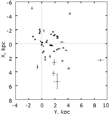
Fig. 1 shows the space distribution of masers projected onto the Galactic plane. The objects can be seen to be widely scattered along the , coordinates, implying a large scatter of position angles. Hence the spectrum analysis algorithm has to be constructed in order to correctly extract periodic signal from velocity perturbations traced by masers.
5 Results
First, we re-determined the parameters of the Galactic rotation curve using the data for 58 masers. The method employed is based on the well-known Bottlinger formulae (Ogorodnikov, 1965), where the angular velocity of Galactic rotation is expanded into a series up to 2-nd order terms in (Bobylev & Bajkova 2010). We adopt kpc and infer the following components of the peculiar solar velocity: km c-1, and the following parameters of the Galactic rotation curve: km c-1 kpc -1, km c-1 kpc -2, km c-1 kpc -3. The linear Galactic rotation velocity at then is equal to: km c-1.
There is good agreement of our results with the results of analyzing masers by different authors. Based on a sample of 18 masers, McMillan & Binney (2010) showed that lying within the range km s-1 kpc-1 at various was determined most reliably and obtained an estimate of km s-1 for kpc. Based on a sample of 18 masers, Bovy, Hogg & Rix (2009) found km s-1 at kpc. Using 44 masers, Bajkova & Bobylev (2012) found: km s-1, km s-1 kpc-1, km s-1 kpc-2, km s-1 kpc-3, km s-1.
It is important that the rotation-curve parameters found are in good agreement with the results of analyzing young Galactic disk objects rotating most rapidly around the center: OB associations with km s-1 kpc-1 (Mel’nik, Dambis, & Rastorguev 2001; Mel’nik & Dambis 2009), blue supergiants with km s-1 kpc-1 and km s-1 kpc-2 (Zabolotskikh, Rastorguev & Dambis 2002), or OB3 stars with km s-1 kpc-1, km s-1 kpc-2 and km s-1 kpc-3 (Bobylev & Bajkova 2011).
The galactocentric radial, and tangential, ( velocities of the masers were determined from the relations
| (26) |
| (27) |
where are the heliocentric space velocities adjusted for solar peculiar motion.
The residual tangential velocities are obtained from the tangential velocities (26) minus the smooth rotation curve that is defined by the Galactic rotation parameters and found. The radial velocities (27) depend only on one Galactic parameter and do not depend on the rotation curve. As our experience showed, the data are so far insufficient to reliably extract the density wave from the tangential residual velocities of the masers. Therefore, here we determine the spiral density wave parameters only from galactocentric radial velocities.
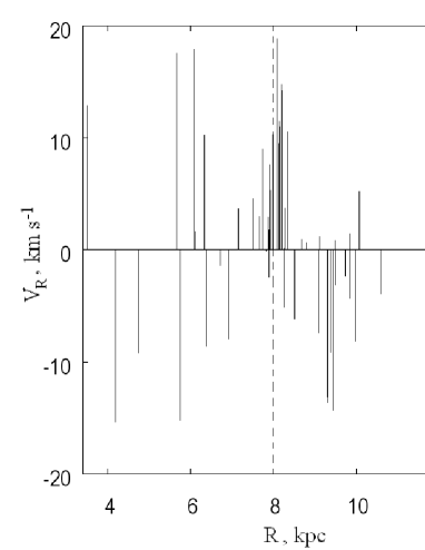
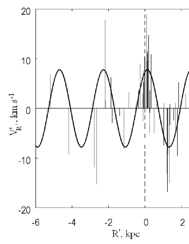
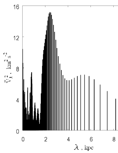
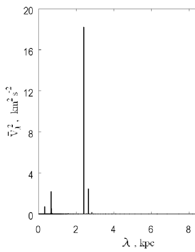
Figure 2 shows the input radial velocity series . Figure 3 shows transformed velocity series and main extracted harmonic. The periodogram obtained using a modified Fourier transform-based method is given in fig. 4. An analysis of this periodogram allowed us to estimate the following spiral wave parameters: the amplitude of the radial perturbations km c-1; the wavelength (interarm distance in the galactocentric direction) kpc, and the phase of the Sun in the spiral density wave . The pitch angle of the spiral wave estimated from equation (5) for is . The significance level of the peak is . Significance level was estimated using the simplest method based on Schuster theorem (Vityazev, 2001).The error bars are based on a Monte-Carlo simulation of 1000 random realizations of input data assuming that measurement errors obey the normal distribution. Note that the value for found by fitting the harmonic with kpc to data is in good agreement with relation (21).
Power spectrum, obtained using the GMEM, is shown in fig. 5. As we can see, this nonlinear reconstruction algorithm allowed us to get rid of the side lobes near the main peak almost completely and, thus, to increase considerably the significance of the extracted periodicity with kpc.
For comparison, in our previous study (Bajkova & Bobylev 2012) we have obtained from data on 44 masers the following spiral density wave parameters: amplitude km s-1, wavelength kpc, pitch angle , and the phase of the Sun .
The parameters of Galactic spiral density wave obtained are in good agreement with those found by different authors by applying different methods to different Galactic tracer objects (Mel’nik et al. 2001; Zabolotskikh et al. 2002; Bobylev & Bajkova 2011 and many others).
6 Conclusions
We used both Fourier transform-based spectral analysis technique and the generalized maximum entropy reconstruction method to extract a periodic signal from the galactocentric radial velocities of 58 masers with currently known high-precision trigonometric parallaxes, proper motions and line-of-site velocities. In accordance with Lin & Shu (1964) theory, the extracted periodic signal is associated with the Galactic spiral density wave. Masers span a wide range of galactocentric distances R kpc and show a large scatter of position angles in the Galactic plane, making it necessary an exact accounting for both the logarithmic nature of the argument and position angles. As a result, we re-determined the main parameters of the Galactic spiral density wave as follows: amplitude of radial velocities perturbations km s-1, wavelength kpc, pitch angle and phase of the Sun in the density wave .
Acknowledgements.
This work was supported by the “Non - stationary processes in the Universe” Program of the Presidium of the Russian Academy of Science and the Program of State Support for Leading Scientific Schools of the Russian Federation (project. NSh–16245.2012.2, “Multi-wavelength Astrophysical Studies”).References
- [1] Bajkova, A.T.: 1992, Astron. & Astroph. Tr. 1, 313
- [2] Bajkova, A.T., Bobylev, V.V.: 2012, Astron. Lett. 38, 549
- [3] Bobylev, V.V., Bajkova, A.T.: 2011, Astron. Lett. 37, 526
- [4] Bobylev, V.V., Bajkova, A.T.: 2010, Mon. Not. R. Astron. Soc. 408, 1788
- [5] Bobylev, V.V., Bajkova, A.T., Stepanishchev, A.S.: 2008, Astron. Lett., 34, 515
- [6] Bovy, J., Hogg, D. W., Rix, H.-W.: 2009, Astrophys. J. 704, 1704
- [7] Clemens, D.P.: 1985, Astrophys. J. 295, 422
- [8] Frieden, B.R., Bajkova, A.T.: 1994, Appl. Opt. 33, 219
- [9] Honma, M., Bushimata, T., Choi, Y.: 2007, Publ. Astron. Soc. Jpn. 59, 889
- [10] Lin, C.C., Shu, F.H.: 1964, Astroph. J. 140, 646
- [11] McMillan, P.J., Binney, J.J.: 2010, Mon. Not. R. Astron. Soc. 402, 934
- [12] Mel’nik, A.M., Dambis, A.K.: 2009, Mon. Not. R. Astron. Soc. 400, 518
- [13] Mel’nik, A.M., Dambis, A.K., Rastorguev, A.S.: 2001, Astron. Lett. 27, 521
- [14] Ogorodnikov, K.F.: 1965, Dynamics of Stellar Systems, Pergamon, Oxford
- [15] Reid, M.J., Menten, K.M., Zheng, X.W., Brunthaler, L., Moscadelli, L., Xu, Y.: 2009, Astrophys. J. 700, 137
- [16] Rygl, K.L.J., Brunthaler, A., Reid, M.J., Menten, K.M., van Langevelde, H.J., Xu, Y.R: 2010, Astron. & Astrophys. 511, A2
- [17] Vityazev, V.V.: 2001, Analysis of non-uniform time series, Saint-Petersburg State University press
- [18] Zabolotskikh, M.V., Rastorguev, A.S., Dambis, A.K.: 2002, Astron. Lett. 28, 454