The dark side of the $\mu$: on multiple solutions to renormalisation group equations, and why the CMSSM is not necessarily being ruled out

Abstract

When solving renormalisation group equations in a quantum field theory, one often specifies the boundary conditions at multiple renormalisation scales, such as the weak and grand-unified scales in a theory beyond the standard model. A point in the parameter space of such a model is usually specified by the values of couplings at these boundaries of the renormalisation group flow, but there is no theorem guaranteeing that such a point has a unique solution to the associated differential equations, and so there may exist multiple, phenomenologically distinct solutions, all corresponding to the same point in parameter space. We show that this is indeed the case in the constrained minimal supersymmetric standard model (CMSSM), and we exhibit such solutions, which cannot be obtained using out-of-the-box computer programs in the public domain. Some of the multiple solutions we exhibit have CP-even lightest Higgs mass predictions between 124 and 126 GeV. Without an exhaustive 11-dimensional MSSM parameter scan per CMSSM parameter point to capture all of the multiple solutions, CMSSM phenomenological analyses are incomplete.

1 Introduction

It is a truth universally acknowledged, that renormalisation group (RG) flows are unique, once a boundary condition for each coupling involved in the flow has been specified.

Like many universally acknowledged truths, this one is not necessarily acknowledged in the Universe inhabited by mathematicians. Indeed, the closest one can get in terms of a theorem (called Cauchy–Lipschitz by francophones, but due to Picard–Lindelöf Lindelhof ) concerns the uniqueness (and existence) of the solution to the initial value problem of a sufficiently well-behaved system of differential equations in a neighbourhood of the starting point. There are many situations in physics where these conditions are not satisfied and so the issue of non-uniqueness (as well as non-existence) rears its ugly head.

One physical situation where non-uniqueness is manifest arises in Sturm-Liouville problems, namely linear, second-order, ordinary differential equations (ODEs) with homogeneous boundary conditions specified on either side of an interval. These may be thought of as a pair of first-order ODEs and, as every undergraduate knows, there exists either 1 (namely 0) or infinitely many solutions (namely an eigenfunction multiplied by an arbitrary constant) depending on whether the ODEs correspond to an eigenvalue or not.

A different example, involving RG flows, is pertinent right now at the Large Hadron Collider (LHC). Disciples of high-scale supersymmetric models (rapidly becoming an endangered species) wish to know whether their models are ruled out or not. These models typically impose a large degree of unification of the parameters of e.g. the Minimal Supersymmetric Standard Model (MSSM) at a high energy scale, be they gauge couplings, soft supersymmetry (SUSY) breaking masses, or whatever. Such constraints play the rôle of boundary conditions at one end of the RG flow. The MSSM is then further constrained at the weak scale where various Standard Model measurements, such as the mass of the Z boson, also play the rôle of boundary conditions. The RG equations (RGEs) are non-linear ODEs, for which a solution satisfying both sets of boundary conditions is to be found.

For concreteness, let us imagine an $n$-parameter flow (with $n$ of $O(10^{2})$ in the MSSM), in which $k$ measurements are performed at low energy, and there are $l$ unification conditions at high energy. One may then attempt to answer the question of whether the theory is ruled out or not in the following way: choose values of $n-k-l$ of the unified parameters at high energy, and call those values a ‘point in the parameter space of the model’. Given that $n$ boundary conditions have now been specified, and invoking the aforementioned universally-acknowledged truth that the flow is unique, one may find ‘the’ flow that satisfies the given boundary conditions, by means of a numerical iterative algorithm. The resulting flow then predicts the values of all particle masses and couplings of the theory, including those which have yet to be measured, but are subject to limits (e.g. limits on superpartner masses from LEP and LHC). If the limits are violated, the point in parameter space is ruled out. Finally, one can scan over points in parameter space ad nauseam.

The problem with this approach is that no theorem guarantees that a solution found in this way is unique. (Indeed, the similarity with a Sturm-Liouville problem suggests the contrary.) Thus, there may be more than one trajectory satisfying the boundary conditions, each of which reproduces the unification conditions and the measured Standard Model parameters, but each of which may have completely different values of the as-yet unmeasured low-energy parameters. Some of these may be ruled out and some may not.

This raises the spectre (horrifying or enchanting depending on one’s spiritual taste) that points in the parameter space of, e.g., the CMSSM that have previously been ruled out, are in fact not ruled out at all, because there are multiple RG flows that correspond to the same point in CMSSM input parameter space, with one or more flows still allowed and yet not found by existing algorithms.

In what follows, we shall find multiple RG flows corresponding to the same CMSSM input parameter point. Though our numerical calculations hint that such points may be uncommon, it will become clear that we have no way of exhaustively categorising them. This, unfortunately, makes it rather difficult to say whether some regions of some high scale SUSY breaking scheme, e.g., the CMSSM, are ruled out or not.

Before doing all this, we first try to convince the reader, in § 2, of the existence of multiple solutions for a rather more simple RG flow, namely the flow in the neighbourhood of the Berezinski-Kosterlitz-Thouless (BKT) phase transition. Then, in § 3, we exhibit and investigate the phenomenon for the CMSSM. It is not our purpose here to perform any detailed phenomenology. Rather, we content ourselves with pointing out the existence and prevalence of multiple solutions in the CMSSM parameter space and investigating a few of their properties. We discuss the implications and context of our results in § 4.

2 Toy example: The BKT phase transition

To find a tractable example of the phenomenon of multiple solutions, we consider a system of RGEs with just two couplings, which is the minimal case in which the notion arises of imposing boundary conditions at different scales.

A suitable example is the RG flow corresponding to the BKT phase transition Berezinsky:1970fr ; Kosterlitz:1973xp . This phase transition was first studied in the context of the 2-d XY model in condensed matter physics and can be used to describe superfluid films and arrays of Josephson junctions. It also appears in particle physics in the deconfinement phase transition in compact $U(1)$ gauge theory in $2$ space dimensions, where Polyakov showed long ago Polyakov:1976fu that vortex configurations of the gauge field lead to confinement at zero temperature. The finite-temperature deconfinement phase transition was shown to be of BKT type by embedding in the Georgi-Glashow model Svetitsky:1982gs ; Agasian:1997wv and also by a variational analysis Gripaios:2002xb .

The BKT phase transition is rather special in that it exhibits a line of fixed points ending in a critical point; in the neighbourhood of this point, the RGEs may be written in the form

$$\frac{dx}{dt} =y^{2},$$

$$\frac{dy}{dt} =xy.$$ (1)

These equations may be solved easily enough by a mathematical beginner, but physicists who know more than is good for them may find it amusing to convert the problem to a mechanical one, in the following way. The RGEs do not form a Hamiltonian system (since $\partial_{x}y^{2}\neq-\partial_{y}xy$), but may be turned into one by the non-canonical transformation $y=e^{z}$. Then $\dot{z}=x$ and $\dot{x}=e^{2z}$, such that we may think of a particle of unit mass and momentum $x$ moving in the potential $-\frac{1}{2}e^{2z}$. The Lagrangian is $t$-independent and the conserved energy is, á la Nöther, $E=\frac{1}{2}(x^{2}-e^{2z})=\frac{1}{2}(x^{2}-y^{2})$. In other words, the trajectories are hyperbolae in the $(x,y)$ plane. Moreover, $t$-translation invariance implies that the conditions for the existence of solutions to the boundary value problem can depend only on the difference, $t_{1}-t_{0}$, between the initial and final times.

There is, in addition, a symmetry of the equations of motion that is not a symmetry of the Lagrangian, and therefore does not imply a conserved charge. This symmetry is the rescaling $(x,z,t)\rightarrow(\alpha x,z+\alpha,\alpha^{-1}t)$. This symmetry implies that we can, without loss of generality, always rescale a finite time interval to be unity, $t_{1}-t_{0}=1$.

The form of the potential, $-\frac{1}{2}e^{2z}$, indicates that the momentum, $x$, must increase monotonically with $t$. There are thus 3 types of trajectory, as follows. Trajectories with $x(t_{0})<0$ and positive energy, $x^{2}-y^{2}>0$, proceed inevitably to $z\rightarrow-\infty$, i.e. $y=0$, in time $-\int^{-\infty}\frac{dz}{\sqrt{2E+e^{2z}}}\rightarrow\infty$. Trajectories with $x(t_{0})<0$ and $x^{2}-y^{2}<0$ eventually turn around and proceed to $z\rightarrow+\infty$ in time $\int^{\infty}\frac{dz}{\sqrt{2E+e^{2z}}}<\infty$, as do trajectories with $x(t_{0})\geq 0$. The trajectories are thus as shown in grey in Fig. 1.

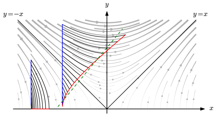
Figure 1: Phase diagram and RG trajectories for the BKT system. The equations enjoy a scale invariance, so the figure has the same character at all scales. The phase diagram is indicated by the background flow-lines (in grey). We show (in black) two distinct sets of flows, with each beginning at a fixed value of $x$ on a blue line, and ending after a fixed interval of time, $\Delta t$, on a red line. For the flows ending on the curved red line, $\Delta t$ is finite, and multiple solutions are indicated by the intersection of this red line with the straight, dashed green line. For the flows ending on the horizontal red line, $\Delta t$ is infinite.

It is apparent from the above discussion that the initial value problem is well defined for any finite starting point $(x(t_{0}),y(t_{0}))$ and finite time interval, but we wish to consider instead the mixed boundary value problem with, say, $x(t_{0})=-a$ and $y(t_{1})=b$. It is immediately evident that the existence of a line of fixed points permits infinitely many solutions to the boundary value problem with $b=0$ on an infinite interval: all trajectories with $x(t_{0})=-a,y(t_{0})<a$ will arrive at the fixed line $y(t_{1}\rightarrow\infty)=0$. This situation is depicted in Fig. 1 by the mapping of the smaller blue line to the horizontal red line.

We are more interested in multiple solutions on a finite time interval. One can show (by straightforward, but tedious, consideration of the explicit solutions to Eq. (2)) that these never arise for boundary conditions of the specific form $x(t_{0})=-a$ and $y(t_{1})=b$. To find multiple solutions on a finite time interval, we need to consider more general boundary conditions. Consider, for example, boundary conditions in which we fix $x$ at $t_{0}$, and fix some (inhomogeneous) linear combination of $x$ and $y$ at time $t_{1}$, say $\alpha x(t_{1})+\beta y(t_{1})=c$. It is then easy to see that multiple solutions must arise for particular choices of $\alpha$, $\beta$ and $c$. Indeed, consider all flows that satisfy $x(t_{0})=-a$, for some other value of $a$, as per the longer blue line in Fig 1. If the flow were linear, the straight line $x(t_{0})=-a$ would be mapped into another straight line at $t=t_{1}$, which would intersect once with the linear combination appearing in the boundary condition. (In special cases such as homogeneous boundary conditions, $a=c=0$, there will be 1 or infinitely many intersections, as for a Sturm-Liouville problem.) But since the flow is non-linear, the line $x(t_{0})=-a$ is mapped to a curve (shown in red), which will intersect multiple times with a suitably chosen straight line (shown in green) corresponding to the boundary condition at $t=t_{1}$. Since, we have effectively converted the boundary value problem into an initial value problem for each point on the blue line, for which the RG flow is known to be unique, the number of solutions to the original boundary value problem is simply given by the number of intersections of the red curve with the green line.

Notice how, in this way, we convert the problem of finding multiple solutions of a system of differential equations (the RGEs) into a problem of finding multiple solutions of a system of algebraic equations (namely the intersections of the line and curve in Fig.1). This makes it relatively straightforward to establish the existence of multiple solutions for a more general system (though we still need to be able to solve the non-linear RGEs of the modified problem in order to do so): we relax one final, say, boundary condition, find the resulting flow for many initial values of a coupling that is not fixed initially, and finally reject flows that do not satisfy the final boundary condition of the original problem. If multiple flows remain, then the original problem has multiple solutions.

It is a much harder problem, in general, to count the total number of solutions for a given system of RGEs and boundary conditions. It can be done, in principle, by relaxing all of the final boundary conditions and instead scanning over all possible initial values of parameters that are not fixed by the initial boundary conditions of the original problem. In this way, we convert the original problem to an initial value problem, for which uniqueness of the flow is guaranteed (assuming the equations are sufficiently well-behaved) by a theorem.

While this is certainly easy enough for a 2-parameter flow as above, it is out of the question for the CMSSM in which, as we will see, we would have to scan over 11 GUT-scale MSSM parameters for a single point in CMSSM parameter space. Thus we cannot be sure of finding all solutions, and therefore it is essentially impossible for us to conclusively declare that a generic point in the CMSSM parameter space is ruled out, in the absence of a theorem on the number of solutions.

The CMSSM is, moreover, further complicated by three features. Firstly, there are really three ‘endpoints’ to the flow, namely the GUT, SUSY, and weak scales. Secondly, some of the boundary conditions simultaneously specify the locations of the endpoints themselves, as well as the values that the Lagrangian parameters take at those endpoints. Thirdly, the boundary conditions are themselves non-linear relations among the Lagrangian parameters, meaning that multiple solutions could arise even if the RGEs were linear. Nevertheless, we can identify multiple solutions easily enough in the following way. Given an algorithm that finds one solution, relax one of the boundary conditions (as we did for the BKT example) and scan over one of the couplings appearing in it, finding one solution for each point. If more than one of these points satisfies all of the original BCs, then the original problem has multiple solutions.

3 Multiple solutions in the CMSSM

The CMSSM Fayet:1 ; Fayet:2 ; Fayet:3 ; Fayet:4 ; Georgi:1 is a softly broken model of supersymmetric field theory, with boundary conditions at three scales and is therefore subject to the possibility of several discrete solutions, even though the number of boundary conditions plus the number of input parameters is equal to the number of free parameters. It remains the phenomenologically most studied example of assumptions about supersymmetry breaking terms in the MSSM, and is still of high interest. In this section, we will find some of its multiple solutions, map out the regions of parameter space in which we can find multiple solutions, and illustrate their properties. However, as we have already discussed, we can by no means guarantee that we have found all of its solutions.

The CMSSM has the following parameters: $\tan\beta$, the ratio of the two Higgs vacuum expectation values; sign$(\mu)$, the sign of a parameter in the MSSM superpotential; $m_{0}$, which is equal to the SUSY breaking family and flavour universal scalar mass terms in the Lagrangian; $M_{1/2}$, which is equal to the gaugino mass SUSY breaking mass parameters; and $A_{0}$, which sets the SUSY breaking trilinear scalar couplings (these are equal to the analogous Yukawa matrix multiplied by $A_{0}$). The soft SUSY breaking terms are nearly all set at the GUT scale, which is defined to be the scale where the gauge couplings are unified, typically $\sim 2-3\times 10^{16}$ GeV. Usually, one expects to obtain two solutions: one for each sign of $\mu$, although occasionally one runs up against physical boundaries (such as an unstable electroweak minimum), and one or both of these solutions is unphysical.

In fact, multiple solutions in the mSUGRA model Cremmer:1978iv ; Cremmer:1978hn ; Barbieri:1982eh have already been found by Drees and Nojiri Drees:1991ab . The mSUGRA model is equivalent to the CMSSM with one additional constraint on a Higgs potential parameter: $m_{3}^{2}(M_{\text{GUT}})=\mu(M_{\text{GUT}})(A_{0}-m_{0})$. Drees and Nojiri used this additional constraint to predict $\tan\beta$ from the minimisation of the weak scale Higgs potential. The resulting equation was analytically shown to be a cubic in $\tan\beta$, which may have up to three physically distinct solutions.

3.1 CMSSM boundary conditions

Before giving the boundary conditions in some detail, we provide a rough sketch of them (and of a resulting RG flow) in Fig. 2 for a certain CMSSM point. Black dots show the boundary conditions: at the low scale, we have boundary conditions on gauge and Yukawa couplings coming from experimental data. In the Figure, $M_{\text{SUSY}}$ is the scale at which superparticle masses are calculated and the Higgs potential is minimised. Thus, at $M_{\text{SUSY}}$, we have a boundary condition on $\mu(M_{\text{SUSY}})$ coming from the Higgs potential minimisation. At the high renormalisation scale, we have a boundary condition on the SUSY breaking terms (we have illustrated this with the gaugino masses $M_{i}$). The high scale itself, $M_{\text{GUT}}$, is usually set to be the scale $Q$ at which $g_{1}(Q)=g_{2}(Q)$, providing another boundary condition ($g_{3}(M_{\text{GUT}})$ is close to these, but not exactly unified in the MSSM; this small discrepancy can easily be explained by GUT threshold corrections Yamada ; Altarelli:2000fu ). The boundary conditions are linked by the RG flow, a set of differential equations in these variables.

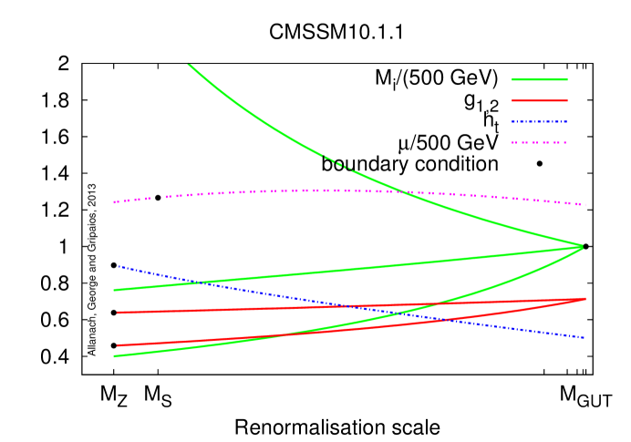
Figure 2: Boundary conditions and renormalisation group flow at CMSSM10.1.1 AbdusSalam:2011fc . The abscissa is a logarithmic scale.

The RG equations of the MSSM are non-linear, coupled, homogeneous first order equations. For example, at one-loop order we have equations governing the evolution of the two Higgs soft SUSY breaking mass parameters $m_{H_{1}}$ and $m_{H_{2}}$ of the form Martin:1993zk

$$16\pi^{2}\frac{\partial m_{H_{2}}^{2}}{dt} = 6\left[(m_{H_{2}}^{2}+m_{{\tilde{Q}}_{3}}^{2}+m_{{\tilde{u}}_{3}}^{2}+A_{t}^{2})h_{t}^{2}\right]-6g_{2}^{2}M_{2}^{2}-\frac{6}{5}g_{1}^{2}M_{1}^{2}+\frac{3}{5}g_{1}^{2}\left(m_{H_{2}}^{2}-m_{H_{1}}^{2}+\right.$$ (2)

$$\left.\mbox{Tr}[m_{\tilde{Q}}^{2}-m_{\tilde{L}}^{2}-2m_{\tilde{u}}^{2}+m_{\tilde{d}}^{2}+m_{\tilde{e}}^{2}]\right),$$

$$16\pi^{2}\frac{\partial m_{H_{1}}^{2}}{dt} = 6\left[(m_{H_{1}}^{2}+m_{{\tilde{Q}}_{3}}^{2}+m_{{\tilde{d}}_{3}}^{2}+A_{b}^{2})h_{b}^{2}\right]-6g_{2}^{2}M_{2}^{2}-\frac{6}{5}g_{1}^{2}M_{1}^{2}-\frac{3}{5}g_{1}^{2}\left(m_{H_{2}}^{2}-m_{H_{1}}^{2}+\right.$$ (3)

$$\left.\mbox{Tr}[m_{\tilde{Q}}^{2}-m_{\tilde{L}}^{2}-2m_{\tilde{u}}^{2}+m_{\tilde{d}}^{2}+m_{\tilde{e}}^{2}]\right),$$

where $t=\ln Q$. There are other similar equations for each of the quantities on the right-hand side of Eq. (3).

We specify our boundary conditions explicitly below for: the Yukawa couplings of the top, bottom, and tau, viz. $h_{t}$, $h_{b}$, and $h_{\tau}$, respectively; the 3 MSSM gauge couplings, $g_{i}$, $i\in\{1,2,3\}$; the various SUSY breaking scalar masses, $m_{\varphi}$; the gaugino masses, $M_{i}$, $i\in\{1,2,3\}$; and for the SUSY breaking trilinear scalar couplings for top, bottom, and tau, $A_{t},A_{b}$ and $A_{\tau}$. Other boundary conditions include those on the parameter $\mu$ appearing in the superpotential $W\supset\mu\hat{H}_{1}\hat{H}_{2}$, and on $m_{3}^{2}$, that mixes the two Higgs doublets in the potential $V\supset m_{3}^{2}H_{2}H_{1}$. These last two boundary conditions come from the minimisation of the Higgs potential with respect to the neutral components of $H_{1}$ and $H_{2}$.

In all, we have the boundary conditions

$$\tan\beta(M_{Z}) = \tan\beta(\mbox{input})$$ (4)

$$h_{t}({M_{Z}}) = \frac{m_{t}(M_{Z})\sqrt{2}}{v(M_{Z})\sin\beta},\qquad h_{b,\tau}(M_{Z})=\frac{m_{b,\tau}(M_{Z})\sqrt{2}}{v(M_{Z})\cos\beta},$$ (5)

$$v(M_{Z}) = 2\sqrt{\frac{{M_{Z}^{2}(\mbox{exp})+\Pi_{ZZ}^{T}(M_{Z})}}{{\frac{3}{5}g_{1}^{2}(M_{Z})+g_{2}^{2}(M_{Z})}}}$$ (6)

$$g_{1}(M_{Z}) = g_{1}(\mbox{exp}),\qquad g_{2}(M_{Z})=g_{2}(\mbox{exp}),\qquad g_{3}(M_{Z})=g_{3}(\mbox{exp}).$$ (7)

$$M_{\text{SUSY}} = \sqrt{m_{{\tilde{t}}_{1}}(M_{\text{SUSY}})m_{{\tilde{t}}_{2}}(M_{\text{SUSY}})}$$ (8)

$$\mu^{2}(M_{\text{SUSY}}) = \frac{m_{\bar{H}_{1}}^{2}(M_{\text{SUSY}})-m_{\bar{H}_{2}}^{2}(M_{\text{SUSY}})\tan^{2}\beta(M_{\text{SUSY}})}{\tan^{2}\beta(M_{\text{SUSY}})-1}-\frac{1}{2}M_{Z}^{2}(M_{\text{SUSY}})$$ (9)

$$m_{3}^{2}(M_{\text{SUSY}}) = \frac{\sin{2\beta(M_{\text{SUSY}})}}{2}\left(m_{\bar{H}_{1}}^{2}(M_{\text{SUSY}})+m_{\bar{H}_{2}}^{2}(M_{\text{SUSY}})+2\mu^{2}(M_{\text{SUSY}})\right)$$ (10)

$$g_{1}(M_{\text{GUT}}) = g_{2}(M_{\text{GUT}})$$ (11)

$$M_{1}(M_{\text{GUT}}) = M_{2}(M_{\text{GUT}})=M_{3}(M_{\text{GUT}})=M_{1/2}$$ (12)

$$m_{\tilde{u}}^{2}(M_{\text{GUT}}) = m_{\tilde{d}}^{2}(M_{\text{GUT}})=m_{\tilde{e}}^{2}(M_{\text{GUT}})=m_{\tilde{L}}^{2}(M_{\text{GUT}})=m_{\tilde{Q}}^{2}(M_{\text{GUT}})=m_{0}^{2}I_{3}$$ (13)

$$m_{H_{1}}^{2}(M_{\text{GUT}}) = m_{H_{2}}^{2}(M_{\text{GUT}})=m_{0}^{2}$$ (14)

$$A_{\tilde{u}}(M_{\text{GUT}}) = A_{0}I_{3},\qquad A_{\tilde{d}}(M_{\text{GUT}})=A_{0}I_{3},\qquad A_{\tilde{e}}(M_{\text{GUT}})=A_{0}I_{3}.$$ (15)

The running parameters in Eqs. (4)-(15) are in the modified dimensional reduction (DRED) scheme Capper:1979ns . The ‘(exp)’ denotes that the value derives from experimental data. We have labelled the input parameter $\tan\beta$ as $\tan\beta(\mbox{input})$. The parameters $m_{b,t,\tau}(M_{Z})$ and $g_{1,2,3}(M_{Z})$ are obtained from experimental data, subtracting loops due to sparticles and Standard Model particles. The Standard Model electroweak gauge couplings $g_{1}(\mbox{exp})$ and $g_{2}(\mbox{exp})$ are fixed by the fine structure constant $\alpha$ and the Fermi constant, $G_{F}$. The values of $g_{i}(\mbox{exp})$ are corrected by one-loop corrections involving sparticles. The parameter $v(M_{Z})\approx 246$ GeV denotes $\sqrt{v_{1}^{2}(M_{Z})+v_{2}^{2}(M_{Z})}$, where $v_{1}$ and $v_{2}$ are the vacuum expectation values of the neutral components of the Higgs doublets $H_{1}$ and $H_{2}$, respectively. The modified DRED $Z^{0}$ boson mass squared is fixed by $M_{Z}^{2}(M_{\text{SUSY}})=v^{2}(M_{\text{SUSY}})\left(\frac{3}{5}g_{1}^{2}(M_{\text{SUSY}})+g_{2}^{2}(M_{\text{SUSY}})\right)/4$. $m_{\bar{H}_{i}}^{2}=m_{H_{i}}^{2}-t_{i}/v_{i}$ are fixed by the soft SUSY breaking mass parameters for the Higgs fields $m_{H_{i}}^{2}$, $i\in\{1,2\}$, as well as by the tadpole contributions $t_{i}$ coming from loops. These tadpole contributions have terms linear in $\mu(M_{\text{SUSY}})$ as well as terms that are logarithmic in it, and so Eq. (9) is not a simple quadratic equation for $\mu(M_{\text{SUSY}})$. $\Pi_{ZZ}^{T}(M_{Z})$ is the MSSM self-energy correction to the $Z^{0}$ boson mass which can be found in Ref. Pierce:1996zz and $I_{3}$ is a 3$\times$3 matrix in family space. For further details, see the SOFTSUSY manual Allanach:2001kg .

Spectrum calculators for the MSSM that are currently in the public domain, namely ISASUSY Baer:1993ae , SOFTSUSY Allanach:2001kg , SPheno Porod:2003um , SUSEFLAV Chowdhury:2011zr and SUSPECT Djouadi:2002ze , solve Eqs. (4)-(15) (or equations very similar to them) and thus find ‘the’ RG flow by fixed point iteration. The particular algorithm used by SOFTSUSY, for example, is shown in Fig. 3.

Figure 3: Iterative algorithm used to calculate the SUSY spectrum. Each step (represented by a box) is described in more detail in the text. The initial step is the uppermost one.

Fixed point iteration can only find at most one solution, for a given starting point: guesses for MSSM parameters are initially input to step (a), and the algorithm is applied. If a self-consistent solution to the whole system of boundary conditions and RG flow is found, the parameters at step (c) remain approximately the same on successive iterations, and the iterative loop is exited, returning a single solution. If we are to find multiple solutions, this iterative algorithm must be modified.

3.2 Finding some multiple solutions

In order to exhibit multiple solutions, we follow the aforementioned prescription of changing the boundary conditions slightly. We leave all of the boundary conditions described above unchanged, except for the one for $\mu({M_{\text{SUSY}}})$, which we allow to be an input parameter instead. Thus we do not apply Eq. (9): instead, we turn it into a prediction $M_{Z}(\mbox{pred})$ for the $Z^{0}$ boson pole mass:

$$M_{Z}^{2}(\mbox{pred}) = 2\left(\frac{m_{\bar{H}_{1}}^{2}(M_{\text{SUSY}})-m_{\bar{H}_{2}}^{2}(M_{\text{SUSY}})\tan^{2}\beta(M_{\text{SUSY}})}{\tan^{2}\beta(M_{\text{SUSY}})-1}-\mu^{2}(M_{\text{SUSY}})\right)$$ (16)

$$+\Pi_{ZZ}^{T}(M_{\text{SUSY}}),$$

where in practice, we use $\Pi_{ZZ}^{T}(M_{\text{SUSY}})=M_{Z}^{2}(\mbox{exp})-M_{Z}^{2}(M_{\text{SUSY}})$. When Eq. (16) agrees with the experimentally determined central value, $M_{Z}(\mbox{exp})=91.1887$ GeV, we have a consistent solution of the system of boundary conditions and renormalisation group equations. Thus, in the algorithm, we supplant Eq. (9) by Eq. (16) in step (d). This is much the same approach as the one we took in the BKT toy example above, in that we have relaxed a boundary condition, viz. Eq. (9), and scanned over a coupling, viz. $\mu({M_{\text{SUSY}}})$, that appeared in it. Our algorithm can still find at most one solution for each value of $\mu({M_{\text{SUSY}}})$, but more than one value of $\mu({M_{\text{SUSY}}})$ might satisfy the original boundary conditions.

We emphasise that, while $\mu(M_{\text{SUSY}})$ is scanned, no other parameters are changed by hand. A change in $\mu(M_{\text{SUSY}})$ changes the neutralino, chargino and third family squark masses. Thus, the SUSY radiative corrections to the top mass will change, and therefore $h_{t}$ via Eq. (5). $h_{t}$, in turn, strongly affects the renormalisation of $M_{H_{i}}^{2}$, thus $M_{H_{i}}^{2}(M_{\text{SUSY}})$ may change, even though $M_{H_{i}}^{2}(M_{\text{GUT}})$ remains fixed by the selected point in the CMSSM parameter space.

We thus use a modified version of SOFTSUSY3.3.7 with the altered algorithm, and Standard Model input parameters as listed in Appendix A. We show $M_{Z}(\mbox{pred})$ as a function of $\mu(M_{\text{SUSY}})$ for one such CMSSM point in Fig. 4. For $\mu<-550$ GeV, there is no physical solution due to the pseudoscalar $A^{0}$ being tachyonic, signalling that the desired electroweak minimum is not present. In the Figure, we see the usual two solutions (one for $\mu>0$ at point B and one for $\mu<0$ at point C, both of which SOFTSUSY3.3.7 finds) plus an additional solution (at the point A) for $\mu<0$. Along the curve, $M_{X}$, gauge and Yukawa couplings, and Higgs soft mass parameters vary, indeed all MSSM parameters that are not boundary conditions, vary.

Figure 4: Multiple solutions in the CMSSM at $m_{0}=2800$ GeV, $M_{1/2}=660$ GeV, $A_{0}=0$ and $\tan\beta=40$. Along the curve, all boundary conditions are applied except for the Higgs potential minimisation condition for $\mu(M_{\text{SUSY}})$, Eq. (9). Where the curve intersects the line $M_{Z}^{2}(\mbox{pred})/M_{Z}^{2}(\mbox{exp})=1$ (marked as A, B and C), there are solutions that are consistent with all of the boundary conditions. The insert shows a zoomed region of the plot.

Between $\mu(M_{\text{SUSY}})=-548$ GeV and $\mu(M_{\text{SUSY}})=-530$ GeV, each term on the right-hand side of Eq. (16) is monotonic, and so it is only their combination that renders the minimum. In particular, it is the combination of the terms within the large brackets, since $M_{Z}^{2}(M_{\text{SUSY}})$ has only a very tiny dependence upon $\mu(M_{\text{SUSY}})$ within its range. We have strong evidence to suggest that there are no other solutions at larger values of $|\mu(M_{\text{SUSY}})|$: there, the second term $-2\mu^{2}(M_{\text{SUSY}})$ in Eq. (16) dominates, and $M_{Z}^{2}(\mbox{pred})$ is negative.

Out-of-the box SOFTSUSY3.3.7 will not find solution A, even if the starting guess for the iteration is changed. This is because the solution is repulsive if one uses the unmodified algorithm depicted in Fig. 3. We have checked this by inputting solution A into the usual SOFTSUSY3.3.7 algorithm and performing some iterations: the algorithm then converges on to solution B. We may consider the usual SOFTSUSY3.3.7 algorithm to be an iterative fixed point algorithm in $\mu$: then, for a solution, we have $\mu_{0}(M_{\text{SUSY}})=f(\mu_{0}(M_{\text{SUSY}}))$, where $f$ is the function that performs one iteration i.e. the ordered steps (d), (e), (a), (b) and (c) in Fig. 3. For some value of $\mu=\mu_{0}(M_{\text{SUSY}})$ corresponding to a solution, in a neighbourhood around the point $\mu_{0}$ the fixed point iteration algorithm is stable if $|df(\mu(M_{\text{SUSY}}))/d\mu(M_{\text{SUSY}})|_{\mu=\mu_{0}}<1$ and unstable if $|df(\mu(M_{\text{SUSY}}))/d\mu(M_{\text{SUSY}})|_{\mu=\mu_{0}}>1$. We calculate $f(\mu_{0}(M_{\text{SUSY}}))$ numerically by first performing the modified iterative algorithm to calculate $\mu_{0}$, then running one standard SOFTSUSY iteration upon the result. This allows a numerical determination: indeed $|df(\mu(M_{\text{SUSY}}))/d\mu(M_{\text{SUSY}})|=7.4,0.3,0.3$ for solutions A, B and C, respectively, demonstrating again that A is unstable with respect to fixed point iteration, whereas B and C are stable.

The multiple solutions are not due to non-linearities in Eq. (16) alone. We have shown this by taking each of our solutions in turn (say, A) and then scanning over $\mu(M_{\text{SUSY}})$ while not performing the RG flow and not applying the other boundary conditions, calculating $M_{Z}^{2}(\mbox{pred})/M_{Z}^{2}(\mbox{exp})$. This system is observed to have only one solution for a given sign of $\mu$. This is in contrast to the multiple solutions found in a model with an extra constraint (mSUGRA) by Drees and Nojiri Drees:1991ab , where a single boundary condition (namely the one for $\tan\beta$ derived from Eq. 10) displayed multiple solutions in some regions of parameter space.

Fig. 4 displays some non-smooth kinks at $\mu\approx\pm 50$ GeV: these occur when $|M_{\chi_{1}^{0}}|+|M_{\chi_{2}^{0}}|=M_{Z}$. For $|\mu|>50$ GeV, a non-smooth piece is introduced in the one-loop self-energy of the $Z^{0}$, $\Pi_{ZZ}^{T}(M_{\text{SUSY}})$ as the particles in the loop are no longer on-shell. The inverted spike at $\mu(M_{\text{SUSY}})\approx 6$ GeV also is present for other values of $m_{0}$, $M_{1/2}$, $A_{0}$ and $\tan\beta$, and can lead to additional solutions, if it is deep enough. At $\mu(M_{\text{SUSY}})\approx 6$ GeV, the charginos are approaching zero mass, changing the value of the running values of the MSSM electromagnetic coupling as extracted from data. This changes the electroweak couplings, which changes $M_{\text{GUT}}$, significantly changing in turn $m_{H_{2}}^{2}(M_{\text{SUSY}})$ in Eq. (16), which dominates the prediction for $M_{Z}(\mbox{pred})$.

quantity	solution A	solution B	solution C
$\mu(M_{\text{SUSY}})$/GeV	-545	-535	497
$M_{\chi_{1}^{0}}$/GeV	282	282	281
$M_{\chi_{2}^{0}}$/GeV	502	497	471
$M_{\chi_{3}^{0}}$/GeV	558	548	510
$M_{\chi_{4}^{0}}$/GeV	610	605	593
$M_{\chi_{1}^{\pm}}$/GeV	503	497	470
$M_{\chi_{2}^{\pm}}$/GeV	609	604	592
$m_{\tilde{g}}$/GeV	1612	1612	1612
$m_{3}^{2}(M_{\text{SUSY}})/10^{5}$ GeV2	0.800	0.809	1.07
$m_{H_{2}}^{2}(M_{\text{SUSY}})/10^{5}$ GeV2	-1.94	-1.83	-1.42
$h_{t}(M_{\text{SUSY}})$	0.840	0.839	0.836
$A_{t}(M_{\text{SUSY}})$/GeV	-1056	-1057	-1064
$M_{X}/10^{16}$ GeV	1.94	1.93	1.89
$g_{1}(M_{Z})$	0.460	0.470	0.456
$g_{2}(M_{Z})$	0.634	0.640	0.633

Table 1: Differences in CMSSM parameters and spectra for the multiple solutions of the parameter point $m_{0}=2.8$ TeV, $M_{1/2}=660$ GeV, $\tan\beta=40$ and $A_{0}=0$ displayed in Fig. 4. The solutions are found by scanning $\mu(M_{\text{SUSY}})$ and then the rest of the quantities are determined by the iterative algorithm. We display here some masses and parameters of interest for the 3 solutions that predict the correct value of $M_{Z}$. Above the central horizontal line, all masses are pole masses, whereas below the line, all quantities are evaluated in the modified DRED scheme. Out-of-the-box SOFTSUSY3.3.7 finds solutions B and C.

We display the respective spectra of solutions A,B and C in Table 1. The spectra show some notable differences, illustrating the fact that the solutions are physically different, leading to the possibility of their discrimination by collider measurements. Masses whose tree-level values depend upon the value of $\mu$, such as the heavier neutralino and chargino masses, show the largest differences. Other sparticle and Higgs masses do have small per-mille level differences. We also see some differences in the modified DRED scheme running parameters between the solutions. We have found other points in CMSSM parameter space with several solutions where some sparticle masses differ by hundreds of GeV, but the additional solutions had sparticles lighter than $M_{Z}/2$ and were obviously phenomenologically excluded by LEP, which saw no significant evidence for sparticles in millions of $Z^{0}$ decays.

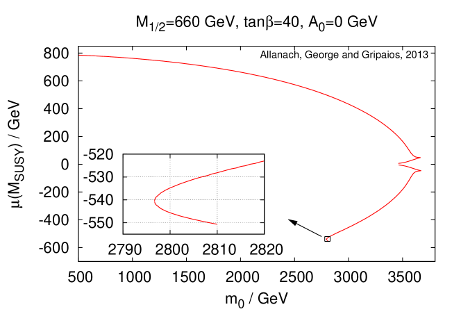
Figure 5: Multiple branches of solutions in the CMSSM at $M_{1/2}=660$ GeV, $A_{0}=0$ GeV and $\tan\beta=40$. Each point on the curve is a solution consistent with all boundary conditions. The value of $m_{0}$ ranges as per the horizontal axis, and corresponds to a horizontal slice through Fig. 7. The curve exhibits a single solution for $m_{0}<2796.7$ GeV and multiple solutions (3 then 2 then 4) as $m_{0}$ increases above this value.

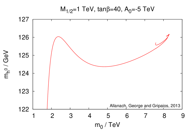
Figure 6: Multiple branches of solutions in the CMSSM at $M_{1/2}=1$ TeV, $A_{0}=-5$ TeV and $\tan\beta=40$. The value of $m_{0}$ ranges as per the horizontal axis. We plot here the predicted values of the Higgs mass, $m_{h^{0}}$. There are 3 solutions in the range $7572\;\text{GeV}\leq m_{0}\leq 7595\;\text{GeV}$ which are consistent with recent LHC measurements of a Higgs boson mass.

The CMSSM parameter point at which we have found our multiple solutions A, B, C is by no means alone. In Fig. 5, we scan in $m_{0}$ as well as $\mu(M_{\text{SUSY}})$ in order to show the appearance and disappearance of various branches of the solutions. We see the appearance of multiple solutions for $m_{0}>2796.7$ GeV, which then collapse to the usual two solutions, one for $\mu>0$ and one for $\mu<0$, when $m_{0}=2810-3400$ GeV. For $m_{0}=3400-3700$ GeV though, there are four solutions. In Fig. 6 we exhibit another point in parameter space that has multiple branches of solutions which predict a CP-even lightest Higgs mass consistent with recent LHC measurements of a Higgs boson ATLAS:2012oga ; Chatrchyan:2012ufa . For $m_{0}=7572-7595$ GeV there are 3 solutions, 2 with $\mu(M_{\text{SUSY}})<0$, which have $m_{h^{0}}$ in the range $125.4$ GeV to $125.7$ GeV.

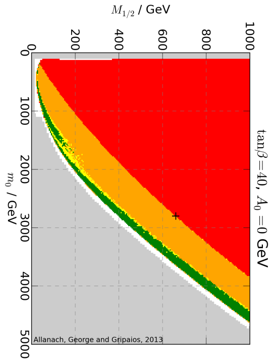
Figure 7: Parameter scan of the CMSSM, with colour indicating number of solutions at a given point: white, red, orange, yellow and green being 0, 1, 2, 3 and 4 solutions respectively. The red region at the top-left has 1 solution for $\mu(M_{\text{SUSY}})>0$ and no solutions for $\mu(M_{\text{SUSY}})<0$. The orange region to the right of this red region has 2 solutions, 1 for each sign of $\mu(M_{\text{SUSY}})$. Further to the right are regions with 3 and 4 solutions. The ‘+’ marks the position of the point detailed in Table 1, and lies on a thin region, difficult to see in between the red and orange regions, which possesses 3 solutions. Phenomenological constraints have not been applied.

We now wish to investigate how prevalent in CMSSM parameter space the multiple solutions are. In Fig. 7, we fix $\tan\beta$ and $A_{0}$, and scan over $m_{0}$ and $M_{1/2}$, showing by colour how many solutions (with either sign of $\mu$) we are able to find at each point. White regions correspond to no solution (because, for example, there is no electroweak symmetry breaking), and red, orange, yellow and green correspond to 1, 2, 3, and 4 solutions, respectively. Grey regions have not been scanned, but the large grey area on the right of the plot is in the usual region of unsuccessful electroweak symmetry breaking, and we expect 0 solutions. The large red region has a single solution for $\mu>0$; in this region there is no solution for $\mu<0$ due to tachyonic $A_{0}$. The orange region has the usual 2 solutions, one for each sign of $\mu$. Beyond this, near the boundary of electroweak symmetry breaking, multiple solutions for both signs of $\mu$ are prevalent. The solutions found near the edge of successful electroweak symmetry breaking correspond to the spiky apex of the curve in Fig. 4 shifting down to intersect the horizontal dotted line in 4 distinct places, corresponding to 4 correct predictions for $M_{Z}$.

Fig. 5 shows the value of $\mu$ for a slice through Fig. 7 at $M_{1/2}=660$ GeV. For low $m_{0}$ we are in the red region and there is only 1 solution. As we increase $m_{0}$, just before entering the region with 2 solutions, we hit a small patch of parameter space which exhibits 3 solutions, 2 of which are for $\mu<0$. The points in parameter space where this occurs are indicated (for those with keen eyesight) in Fig. 7 by the isolated yellow dots between the red and orange regions. We have verified that these regions of 3 multiple solutions are not confined to single points in parameter space, but rather occupy a finite area, as shown by the inset in Fig. 5, and as shown by the small region $m_{0}=7572-7595$ GeV in Fig. 6. It is expected that this area runs the length of the boundary between the red and orange regions. Whilst most of the multiple solutions are fairly near the boundary of electroweak symmetry breaking, there is nevertheless a significant volume of parameter space where the multiple solutions play a rôle, and they should not be ignored in phenomenological analyses.

We have performed further scans of parameter space at selected values of $\tan\beta$ and $A_{0}$, and counted solutions in the $m_{0}$-$M_{1/2}$ plane. The qualitative features of these other slices through the parameter space of the CMSSM are similar to Fig. 7, including the existence of a region with three solutions between the red and orange regions. One occasionally finds small areas, close to the edge of successful electroweak symmetry breaking, that have six solutions, two for $\mu<0$ and four for $\mu>0$. For example, $\tan\beta=20$, $A_{0}=-1000$ GeV, $M_{1/2}=170$ GeV and $m_{0}=2840$ GeV is a point with six such solutions. The regions with three and four solutions occur at larger values of $m_{0}$ close to the region of electroweak symmetry breaking. While the position of the no electroweak symmetry breaking boundary is extremely sensitive to the top quark mass $m_{t}$, so that uncertainties on it remain high Allanach:2000ii ; Allanach:2012qd , we have checked that the additional solutions remain (but move in $m_{0}$) when we change $m_{t}$.

4 Discussion

Quantum field theories with multiple parameters that have boundary conditions imposed at multiple renormalisation scales may admit several physically distinct solutions for the same boundary conditions. Each separate solution corresponds to a different RG trajectory, consistent with the RG flow itself being unique. We have exemplified this analytically with the simple BKT model, and shown the relevance of multiple solutions to high energy physics, where each solution generally corresponds to distinct phenomenology.

Imposing boundary conditions on the CMSSM naturally involves different renormalisation scales, namely the weak scale, $M_{\text{SUSY}}$, and the gauge coupling unification scale. Thus, the CMSSM is a good candidate for a theory possessing several different solutions, for a single set of input parameters sign$(\mu)$, $m_{0}$, $M_{1/2}$, $A_{0}$ and $\tan\beta$. Publicly available computer programs solve for the RG flow using iteration, which finds at most one solution consistent with the boundary conditions, for a given point in the CMSSM parameter space. However, we have shown that multiple, physically distinct solutions exist in extended regions of parameter space due to the multiple boundary nature of the problem. We showed this by relaxing a boundary condition, scanning over the parameter $\mu(M_{\text{SUSY}})$, and (for reasons of computational efficiency) completing the rest of the calculation by iteration. We find additional, previously unknown and unexplored solutions at different values of $\mu(M_{\text{SUSY}})$, which we cryptically referred to in the title as “the dark side of the $\mu$”. However, we might well have found yet more solutions if we had scanned over other parameters, so in reality all of the parameters that are not directly fixed by a BC have just as much of a dark side, waiting to be explored.

In order to be sure of finding all of the solutions, one could turn the boundary value problem into an initial value problem and perform the RG flow in one direction only. One possible method would be to start at the GUT scale and, for a given sign$(\mu)$, $m_{0}$, $A_{0}$, $M_{1/2}$, and $\tan\beta(\mbox{input})$, use $M_{\text{GUT}}$, $\tan\beta(M_{\text{GUT}})$, $g_{1}(M_{\text{GUT}})=g_{2}(M_{\text{GUT}})$, $g_{3}(M_{\text{GUT}})$, $h_{t}(M_{\text{GUT}})$, $h_{b}(M_{\text{GUT}})$, $h_{\tau}(M_{\text{GUT}})$, $\mu(M_{\text{GUT}})$, $m_{3}^{2}(M_{\text{GUT}})$, $v(M_{\text{GUT}})$ and $M_{\text{SUSY}}$ as scanning parameters. This 11-dimensional scan, if performed finely enough, would then find all of the possible solutions that match $g_{1}(\mbox{exp})$, $g_{2}(\mbox{exp})$, $M_{\text{SUSY}}$, $m_{3}^{2}(M_{\text{SUSY}})$, $g_{3}(\mbox{exp})$, $v(M_{Z})$, $m_{b}$, $m_{t}$, $m_{\tau}$, $M_{Z}$ and $\tan\beta(M_{Z})$. Note that we found that even while scanning only in one dimension and finding the rest of the parameters by iteration, some of the low-energy output parameters are rapidly varying functions of the high-energy inputs, so that finding some of the solutions is computationally intensive. This problem would inevitably be more acute for an 11-dimensional scan, and we conclude that it would be extremely difficult to know for sure whether one has found all of the solutions, in the absence of a theorem as to their number.

Here, we have shown examples of phenomenologically viable multiple solutions where some sparticle masses differ by a few per cent between the solutions. However, we have also found other solutions where some sparticle masses differ by order 100%; for example, the 4 solutions in Fig. 5 where $m_{0}\sim 3500$ GeV have this property. Due to light neutralinos and/or charginos, these solutions are phenomenologically excluded, but their existence points to the possibility of phenomenologically viable solutions with large differences in their spectra.

It seems at least plausible, then, that some regions of CMSSM parameter space have been ruled out erroneously, because of the existence of additional solutions, yet to be found, with a phenomenology that is consistent with current bounds. For example, we have seen that neutralinos and chargino masses may differ at the tree-level between the multiple solutions, and so bounds coming from dark matter searches are liable to change, since they are very sensitive to the mass of the dark matter candidate (in this case, the lightest neutralino). Similarly, we have seen in Fig. 6 that the same parameter point can lead to multiple predictions for $m_{h^{0}}$; in the coming era of precision Higgs physics, we may well find points for which the solution found by the standard algorithms is incompatible with the measured $m_{h}$, while other solutions are compatible.

Should we therefore consider all existing exclusions of the CMSSM parameter space as suspect? Fortunately, there are sectors in which we do not expect the phenomenology to be greatly changed for different solutions, such that existing exclusions from experimental searches may be considered robust. Important examples are collider searches for gluinos and squarks decaying into jets and missing energy, which provide powerful constraints upon the CMSSM ATLAS-CONF-2012-109 ; Chatrchyan:2012lia . The gluino/squark production cross-sections relevant for the calculation of these bounds depend upon the gluino and first two-family squark masses. Since these are fixed at the GUT scale by the boundary condition $M_{3}(M_{\text{GUT}})=M_{1/2}$ and $m_{\tilde{q}}(M_{\text{GUT}})=m_{0}$, they only differ between the different solutions at the loop level. Perturbativity implies that these corrections are small, and so one expects that the production cross-sections will not differ greatly between the various solutions. Thus, we expect the previously calculated limits on the CMSSM from squark and gluino production to approximately hold. One significant caveat to this is in regions of parameter space where the ratio of the neutralino mass to the gluino or squark mass differs significantly between solutions. This can significantly change the kinematics of the decay of the gluino and squark, and therefore can affect the acceptance of signal events passing the cuts applied in the experimental analyses.

For the time being, in the absence of a signal for supersymmetry at colliders, multiple solutions add a potential loop hole to some of the exclusion bounds derived in models such as the CMSSM. If evidence for supersymmetry is found in the future, the phenomenon will present a new facet: points in the parameter space of candidate SUSY theories might be incorrectly discarded on the grounds of not being able to explain the signal, when other, unknown solutions, corresponding to the same parameter point, can explain it. We thus might be led in the wrong direction in searching for the correct theoretical description of new physics. Conversely, if all the solutions are known, then we should be able to discriminate between them given sufficient measurements, given that they are physically distinct.

There has been a recent growing industry in multi-dimensional phenomenological fits of parameter space in the CMSSM to collider and astrophysical data (see Refs. Allanach:2005kz ; Buchmueller:2011ab ; Balazs:2012qc ; Cabrera:2012vu ; Fowlie:2012im ; Strege:2012bt for some examples). These fits use either Bayesian or frequentist statistics. The Bayesian fits yield posterior probability densities, which are weighted by the probability masses in marginalised parameters. The addition of multiple CMSSM solutions to these fits would only have a negligible affect if the probability mass associated with the non-standard solutions is negligible. Performing a Bayesian fit with the additional 11 dimensions of our scan would be an interesting exercise, to see what the effect of the multiple solutions is. Such fits, since they scan in $m_{3}^{2}$ and $\mu$ (among other parameters) rather than $\tan\beta$ (and fixing $\mu$ by $M_{Z}(\mbox{exp})$), will implicitly and automatically take into account a Jacobian factor that was calculated for this purpose Allanach:2007qk ; Cabrera:2008tj . Frequentist fits must scan in the additional solution space and may be even more vulnerable to changes if they have a better best-fit point, since parameter estimation always relies on $\Delta\chi^{2}$, the difference in $\chi^{2}$ between the current parameter space point and the best-fit point. It remains to be seen how much these effects will change the fits in each case, but at the moment they remain incomplete without the inclusion of the multiple solutions exhibited here.

Finally, we emphasise that the CMSSM is only one example of a model where the SUSY breaking conditions are mostly set at a scale much higher than the weak scale; we expect other examples to feature multiple solutions as well.

Appendix A Standard Model input parameters

As input parameters, we have PDG $G_{F}=1.16637$ GeV^-2, pole masses $m_{t}=173.5$ GeV, $M_{Z}(\mbox{exp})=91.1887$ GeV and $m_{\tau}=1.77669$ GeV, modified minimal subtraction scheme Standard Model values of: $m_{b}(m_{b})=4.18$ GeV, $\alpha(M_{Z})^{-1}=127.916$, $\alpha_{s}(M_{Z})=0.1187$.

References

- (1) Lindelöf, E., Sur l’application de la méthode des approximations successives aux équations différentielles ordinaires du premier ordre, Comptes Rendus 114 (1894) 454.
- (2) M. Liu and P. Nath, Higgs Boson Mass, Proton Decay, Naturalness and Constraints of LHC and Planck Data, 1303.7472.
- (3) V. Berezinsky, Destruction of long range order in one-dimensional and two-dimensional systems having a continuous symmetry group. 1. Classical systems, Sov.Phys.JETP 32 (1971) 493–500.
- (4) J. Kosterlitz and D. Thouless, Ordering, metastability and phase transitions in two-dimensional systems, J.Phys. C6 (1973) 1181–1203.
- (5) A. M. Polyakov, Quark Confinement and Topology of Gauge Groups, Nucl.Phys. B120 (1977) 429–458.
- (6) B. Svetitsky and L. G. Yaffe, Critical Behavior at Finite Temperature Confinement Transitions, Nucl.Phys. B210 (1982) 423.
- (7) N. O. Agasian and K. Zarembo, Phase structure and nonperturbative states in three-dimensional adjoint Higgs model, Phys.Rev. D57 (1998) 2475–2485 [hep-th/9708030].
- (8) B. Gripaios, Variational analysis of deconfinement in compact U(1) gauge theory, Phys.Rev. D67 (2003) 025023 [hep-th/0211104].
- (9) P. Fayet, Supersymmetry and Weak, Electromagnetic and Strong Interactions, Phys.Lett. B64 (1976) 159.
- (10) P. Fayet, Spontaneously Broken Supersymmetric Theories of Weak, Electromagnetic and Strong Interactions, Phys.Lett. B69 (1977) 489.
- (11) G. R. Farrar and P. Fayet, Phenomenology of the Production, Decay and Detection of New Hadronic States Associated with Supersymmetry, Phys.Lett. B76 (1978) 575.
- (12) P. Fayet, Relations Between the Masses of the Superpartners of Leptons and Quarks, the Goldstino Couplings and the Neutral Currents, Phys.Lett. B84 (1979) 416.
- (13) S. Dimopoulos and H. Georgi, Softly Broken Supersymmetry and , Nucl.Phys. B193 (1981) 150.
- (14) E. Cremmer, B. Julia, J. Scherk, P. van Nieuwenhuizen, S. Ferrara et. al., SuperHiggs Effect in Supergravity with General Scalar Interactions, Phys.Lett. B79 (1978) 231.
- (15) E. Cremmer, B. Julia, J. Scherk, S. Ferrara, L. Girardello et. al., Spontaneous Symmetry Breaking and Higgs Effect in Supergravity Without Cosmological Constant, Nucl.Phys. B147 (1979) 105.
- (16) R. Barbieri, S. Ferrara and C. A. Savoy, Gauge Models with Spontaneously Broken Local Supersymmetry, Phys.Lett. B119 (1982) 343.
- (17) M. Drees and M. M. Nojiri, Radiative symmetry breaking in minimal supergravity with large Yukawa couplings, Nucl.Phys. B369 (1992) 54–98.
- (18) Y. Yamada, From minimal to realistic supersymmetric SU(5) grand unification, Z. Phys. C 60 (1993) 83–94.
- (19) G. Altarelli, F. Feruglio and I. Masina, From minimal to realistic supersymmetric SU(5) grand unification, JHEP 0011 (2000) 040 [hep-ph/0007254].
- (20) S. AbdusSalam, B. Allanach, H. Dreiner, J. Ellis, U. Ellwanger et. al., Benchmark Models, Planes, Lines and Points for Future SUSY Searches at the LHC, Eur.Phys.J. C71 (2011) 1835 [1109.3859].
- (21) S. P. Martin and M. T. Vaughn, Two loop renormalization group equations for soft supersymmetry breaking couplings, Phys.Rev. D50 (1994) 2282 [hep-ph/9311340].
- (22) D. Capper, D. Jones and P. van Nieuwenhuizen, Regularization by Dimensional Reduction of Supersymmetric and Nonsupersymmetric Gauge Theories, Nucl.Phys. B167 (1980) 479.
- (23) B. Allanach, SOFTSUSY: a program for calculating supersymmetric spectra, Comput.Phys.Commun. 143 (2002) 305–331 [hep-ph/0104145].
- (24) H. Baer, F. E. Paige, S. D. Protopopescu and X. Tata, Simulating Supersymmetry with ISAJET 7.0 / ISASUSY 1.0, hep-ph/9305342.
- (25) W. Porod, SPheno, a program for calculating supersymmetric spectra, SUSY particle decays and SUSY particle production at e+ e- colliders, Comput.Phys.Commun. 153 (2003) 275–315 [hep-ph/0301101].
- (26) D. Chowdhury, R. Garani and S. K. Vempati, SUSEFLAV: Program for supersymmetric mass spectra with seesaw mechanism and rare lepton flavor violating decays, Comput.Phys.Commun. 184 (2013) 899–918 [1109.3551].
- (27) A. Djouadi, J.-L. Kneur and G. Moultaka, SuSpect: A Fortran code for the supersymmetric and Higgs particle spectrum in the MSSM, Comput.Phys.Commun. 176 (2007) 426–455 [hep-ph/0211331].
- (28) D. M. Pierce, J. A. Bagger, K. T. Matchev and R.-j. Zhang, Precision corrections in the minimal supersymmetric standard model, Nucl.Phys. B491 (1997) 3–67 [hep-ph/9606211].
- (29) ATLAS Collaboration Collaboration, G. Aad et. al., A particle consistent with the Higgs Boson observed with the ATLAS Detector at the Large Hadron Collider, Science 338 (2012) 1576–1582.
- (30) CMS Collaboration Collaboration, S. Chatrchyan et. al., Observation of a new boson at a mass of 125 GeV with the CMS experiment at the LHC, Phys.Lett. B716 (2012) 30–61 [1207.7235].
- (31) B. Allanach, J. Hetherington, M. A. Parker and B. Webber, Naturalness reach of the large hadron collider in minimal supergravity, JHEP 0008 (2000) 017 [hep-ph/0005186].
- (32) B. Allanach and M. Parker, Uncertainty in Electroweak Symmetry Breaking in the Minimal Supersymmetric Standard Model and its Impact on Searches For Supersymmetric Particles, JHEP 1302 (2013) 064 [1211.3231].
- (33) Search for squarks and gluinos with the atlas detector using final states with jets and missing transverse momentum and 5.8 fb-1 of =8 tev proton-proton collision data, Tech. Rep. ATLAS-CONF-2012-109, CERN, Geneva, Aug, 2012.
- (34) CMS Collaboration Collaboration, S. Chatrchyan et. al., Search for new physics in the multijet and missing transverse momentum final state in proton-proton collisions at TeV, Phys.Rev.Lett. 109 (2012) 171803 [1207.1898].
- (35) B. Allanach and C. Lester, Multi-dimensional mSUGRA likelihood maps, Phys.Rev. D73 (2006) 015013 [hep-ph/0507283].
- (36) O. Buchmueller, R. Cavanaugh, A. De Roeck, M. Dolan, J. Ellis et. al., Higgs and Supersymmetry, Eur.Phys.J. C72 (2012) 2020 [1112.3564].
- (37) C. Balazs, A. Buckley, D. Carter, B. Farmer and M. White, Should we still believe in constrained supersymmetry?, 1205.1568.
- (38) M. E. Cabrera, J. A. Casas and R. R. de Austri, The health of SUSY after the Higgs discovery and the XENON100 data, 1212.4821.
- (39) A. Fowlie, M. Kazana, K. Kowalska, S. Munir, L. Roszkowski et. al., The CMSSM Favoring New Territories: The Impact of New LHC Limits and a 125 GeV Higgs, Phys.Rev. D86 (2012) 075010 [1206.0264].
- (40) C. Strege, G. Bertone, F. Feroz, M. Fornasa, R. R. de Austri et. al., Global Fits of the cMSSM and NUHM including the LHC Higgs discovery and new XENON100 constraints, JCAP 1304 (2013) 013 [1212.2636].
- (41) B. C. Allanach, K. Cranmer, C. G. Lester and A. M. Weber, Natural priors, CMSSM fits and LHC weather forecasts, JHEP 0708 (2007) 023 [0705.0487].
- (42) M. Cabrera, J. Casas and R. Ruiz de Austri, Bayesian approach and Naturalness in MSSM analyses for the LHC, JHEP 0903 (2009) 075 [0812.0536].
- (43) Particle Data Group Collaboration, J. Beringer et. al., Review of Particle Physics (RPP), Phys.Rev. D86 (2012) 010001.