Stability Analysis of Flock and Mill rings for 2nd Order Models in Swarming

G. Albi1, D. Balagué2, J. A. Carrillo3 and J. von Brecht4 1Dipartimento di Matematica e Informatica
Università di Ferrara
Ferrara 44121
Italy.
E-mail: giacomo.albi@unife.it.
2Departament de Matemàtiques, Universitat Autònoma de Barcelona, E-08193 Bellaterra, Spain. E-mail: dbalague@mat.uab.cat. 3Department of Mathematics
Imperial College London
London SW7 2AZ
UK.
E-mail: carrillo@imperial.ac.uk.
4Department of Mathematics, University of California - Los Angeles, Los Angeles, CA 90095, USA. E-mail: jub@math.ucla.edu.
Abstract.

We study the linear stability of flock and mill ring solutions of two individual based models for biological swarming. The individuals interact via a nonlocal interaction potential that is repulsive in the short range and attractive in the long range. We relate the instability of the flock rings with the instability of the ring solution of the first order model. We observe that repulsive-attractive interactions lead to new configurations for the flock rings such as clustering and fattening formation. Finally, we numerically explore mill patterns arising from this kind of interactions together with the asymptotic speed of the system.

DB and JAC were partially supported by the project MTM2011-27739-C04-02 DGI (Spain) and 2009-SGR-345 from AGAUR-Generalitat de Catalunya. JAC acknowledges support from the Royal Society through a Wolfson Research Merit Award. GA acknowledges support from the Università di Ferrara through “Fondi cinque per mille, anno 2009”. JvB acknowledges funding from NSF grant EFRI-1024765 and NSF grant DMS-0907931. This work was supported by Engineering and Physical Sciences Research Council grant number EP/K008404/1.

1. Introduction

Individual-based models (IBMs) appear in biology, mathematics, physics, and engineering. They describe the motion of a collection of N𝑁N individual entities, so the system is defined on a microscopic scale. IBMs are good models for some applications when the number of particles is reasonable. Nonetheless, when the number is large, it is more reasonable to use a continuum model. Some continuum models, like the one in [13, 12], are derived as a mean-field particle limit leading to a mesoscopic kinetic description of the problem. At this level, one looks at the probability density of finding particles at a certain position and velocity at a given time. Several models have been proposed to describe the flocking of birds [8, 28, 4, 27], the formation of ant trails [18], the schooling of fish [21, 7, 5], swarms of bacteria [23], etc.

These models can include some rules that describe the behavior of each individual of the system. Such mechanisms can help to describe the influence of each individual on the others, depending on their relative position and velocity. For instance, one example is the classical three zone model [1, 22]. A three zone model describes how social the individual is in the following sense. If two individuals are too close, they want to have their own space (repulsion). When one individual is far from the group, it wants to go back and socialize (attraction). And finally, in the group, each individual tries to mimic the behavior of the others (orientation). Other models just consider rules for orientation, like the Vicsek model [29, 16]. In this case, there is a mechanism of self-propulsion in which each individual moves with constant speed and adopts the average direction among their local neighbors.

We focus our study in the analysis of two particular examples of IBMs. The first one is a self-propelled interacting particle model that was introduced in [26] and extensively studied in [17, 13]:

{x˙j=vjv˙j=S(|vj|)vj+1Nl=1ljNW(xlxj),j=1,,Nformulae-sequencecasessubscript˙𝑥𝑗subscript𝑣𝑗otherwisesubscript˙𝑣𝑗𝑆subscript𝑣𝑗subscript𝑣𝑗1𝑁superscriptsubscript𝑙1𝑙𝑗𝑁𝑊subscript𝑥𝑙subscript𝑥𝑗otherwise𝑗1𝑁\begin{cases}\displaystyle\dot{x}_{j}=v_{j}\\ \displaystyle\dot{v}_{j}=S(|v_{j}|)v_{j}+\frac{1}{N}\sum_{\begin{subarray}{c}l=1\\ l\neq j\end{subarray}}^{N}\nabla W(x_{l}-x_{j})\end{cases},\quad j=1,\dots,N (1)

We are going to consider the same self-propulsion/ friction term used in [17, 13],

S(|vj|)=αβ|vj|2,α,β>0.formulae-sequence𝑆subscript𝑣𝑗𝛼𝛽superscriptsubscript𝑣𝑗2𝛼𝛽0S(|v_{j}|)=\alpha-\beta|v_{j}|^{2},\qquad\alpha,\beta>0.

Note that such a term gives us an asymptotic speed for the particles, equal to α/β𝛼𝛽\sqrt{\alpha/\beta}. In these references, the authors study (1) with pairwise interaction given by the so-called Morse potential

U(r)=CAer/lACRer/lR,𝑈𝑟subscript𝐶𝐴superscript𝑒𝑟subscript𝑙𝐴subscript𝐶𝑅superscript𝑒𝑟subscript𝑙𝑅U(r)=C_{A}e^{-r/l_{A}}-C_{R}e^{-r/l_{R}},

with CAsubscript𝐶𝐴C_{A}, CRsubscript𝐶𝑅C_{R} denoting the attractive and repulsive strengths and lAsubscript𝑙𝐴l_{A}, lRsubscript𝑙𝑅l_{R} their respective length scales. They find and describe several patterns for the asymptotic behavior in 2D. They observed flocking behavior, mill on a ring, and clustering when particles are milling. In [9], a well-posedness theory is developed for (1) proving the mean-field limit under smoothness assumptions on the potential. The authors show convergence of the particle model toward a measure solution of the kinetic equation.

We perform an analysis on the stability of flock rings and the mill rings as asymptotic solutions for (1). The ring solution was recently studied in [25, 6] where the authors in this work do a careful general linear analysis of the rings for the first order model

X˙j=l=1ljNW(XjXl),j=1,,N.formulae-sequencesubscript˙𝑋𝑗superscriptsubscript𝑙1𝑙𝑗𝑁𝑊subscript𝑋𝑗subscript𝑋𝑙𝑗1𝑁\dot{X}_{j}=\sum_{\begin{subarray}{c}l=1\\ l\neq j\end{subarray}}^{N}\nabla W\left(X_{j}-X_{l}\right),\quad j=1,\dots,N. (2)

Part of the analysis of (2) is used to study the the stability of mill rings in (1), described in [17]. Related pattern formation in the associated first order model has been studied in [30, 24].

Another second order model that we are going to study is

{x˙j=vjv˙j=1Nl=1NH(xjxl)(vlvj)+1Nl=1ljNW(xlxj),j=1,,Nformulae-sequencecasessubscript˙𝑥𝑗subscript𝑣𝑗otherwisesubscript˙𝑣𝑗1𝑁superscriptsubscript𝑙1𝑁𝐻subscript𝑥𝑗subscript𝑥𝑙subscript𝑣𝑙subscript𝑣𝑗1𝑁superscriptsubscript𝑙1𝑙𝑗𝑁𝑊subscript𝑥𝑙subscript𝑥𝑗otherwise𝑗1𝑁\begin{cases}\displaystyle\dot{x}_{j}=v_{j}\\ \displaystyle\dot{v}_{j}=\frac{1}{N}\sum_{l=1}^{N}H(x_{j}-x_{l})(v_{l}-v_{j})+\frac{1}{N}\sum_{\begin{subarray}{c}l=1\\ l\neq j\end{subarray}}^{N}\nabla W(x_{l}-x_{j})\end{cases},\quad j=1,\dots,N (3)

with xj,vj2subscript𝑥𝑗subscript𝑣𝑗superscript2x_{j},v_{j}\in\mathbb{R}^{2} where the velocity vjsubscript𝑣𝑗v_{j} is described by the Cucker-Smale alignment term H𝐻H and the pairwise interaction by a repulsive-attractive radial potential W(x)=k(|x|)𝑊𝑥𝑘𝑥W(x)=k(|x|).

Even if the analysis has been done in full generality for the parameter functions of the model H𝐻H and W𝑊W, we will emphasize the results in some relevant cases. For instance, we consider the case of power law repulsive-attractive potentials [25, 3]

k(r)=raarbb,a>b>0.formulae-sequence𝑘𝑟superscript𝑟𝑎𝑎superscript𝑟𝑏𝑏𝑎𝑏0k(r)=\frac{r^{a}}{a}-\frac{r^{b}}{b},\qquad a>b>0. (4)

For the Cucker-Smale alignment [14, 15, 20, 19, 10], a relevant case is H(x)=g(|x|)𝐻𝑥𝑔𝑥H(x)=g(|x|) with

g(r)=1(1+r2)γ,γ>0.formulae-sequence𝑔𝑟1superscript1superscript𝑟2𝛾𝛾0g(r)=\frac{1}{(1+r^{2})^{\gamma}},\qquad\gamma>0.

The main results of this work show that the flock ring is unstable in the second order models (1) and (3) if and only if its spatial shape is unstable in the first order model (2). We use the same kind of strategy as in [6].

The main idea is to study the stability of the system of ODEs (1) by analyzing the eigenvalues of a suitable linearization with restricted perturbations. We consider particular perturbations of the flock rings in such a way that translational invariance is avoided while preserving the mean velocity. This is really needed since the linearized system associated to (1) is always linearly unstable due to translations. Translational invariance implies the existence of a generalized eigenvector associated to the zero eigenvalue of the matrix defining the linearized system. We characterize all cases in which the linearized system has eigenvalues with zero real part and their consequences in the instability condition. An analysis of the stability of the family of flock solutions is under way in [11].

In addition to flock rings, other spatial shapes are possible as asymptotic solutions. One can also observe flocks on annuli (fattening), lines or points (clustering). These patterns can be explained due to the results in [2].

For the mill ring analysis, we start from the results of [6] to explore other mill configurations that appear with repulsive-attractive potentials. We numerically investigate the formation of fat mills due to the repulsive force and the formation of clusters when varying the asymptotic speed. In addition, we show some switching behaviors between flock and mill rings.

The structure of the paper is as follows. In Section 2 we study the microscopic and the mesoscopic models and we give the definitions of the main objects in our studies, the flock and mill rings. In Section 3 we do a linear stability analysis on the flock rings for models (1) and (3). We also explore the fattening and cluster formation. Finally, in Section 4 we do a similar study on the stability for mill rings. In all sections we have performed several numerical tests supporting our theoretical results.

2. Microscopic & Mesoscopic models

Let us introduce some particular solutions of the particle model (1) and its continuum counterpart.

2.1. Flock and mill solutions: microscopic model

Definition 1.

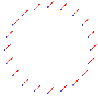
We call a flock ring, the solution of (1) such that {xj}j=1Nsuperscriptsubscriptsubscript𝑥𝑗𝑗1𝑁\{x_{j}\}_{j=1}^{N} are equally distributed on a circle with a certain radius, R𝑅R and {vj}j=1N=u0superscriptsubscriptsubscript𝑣𝑗𝑗1𝑁subscript𝑢0\{v_{j}\}_{j=1}^{N}=u_{0}, with |u0|=α/βsubscript𝑢0𝛼𝛽\left|u_{0}\right|=\sqrt{\alpha/\beta}.

Definition 2.

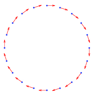
We call a mill ring, the solution of (1) such that {xj}j=1Nsuperscriptsubscriptsubscript𝑥𝑗𝑗1𝑁\{x_{j}\}_{j=1}^{N} are equally distributed on a circle with a certain radius, R𝑅R and {vj}j=1N=uj0=α/βxj/|xj|superscriptsubscriptsubscript𝑣𝑗𝑗1𝑁subscriptsuperscript𝑢0𝑗𝛼𝛽superscriptsubscript𝑥𝑗perpendicular-tosubscript𝑥𝑗\{v_{j}\}_{j=1}^{N}=u^{0}_{j}=\sqrt{\alpha/\beta}\,x_{j}^{\perp}/|x_{j}| with xjsuperscriptsubscript𝑥𝑗perpendicular-tox_{j}^{\perp} the orthogonal vector.

Refer to caption
Refer to caption
Figure 1. Flock and mill ring solutions.

By abuse of notation, we will write |u0|subscript𝑢0\left|u_{0}\right| for |uj0|subscriptsuperscript𝑢0𝑗\left|u^{0}_{j}\right| since |uj0|=α/βsubscriptsuperscript𝑢0𝑗𝛼𝛽\left|u^{0}_{j}\right|=\sqrt{\alpha/\beta} for all j=1,,N𝑗1𝑁j=1,\dots,N. Moreover, we will make use of notation |u0|subscript𝑢0\left|u_{0}\right| for both flock and mill rings indistinctly.

All over the paper, we will identify eiθ(cosθ,sinθ)superscript𝑒𝑖𝜃𝜃𝜃e^{i\theta}\equiv(\cos\theta,\sin\theta) and use x𝑥x to identify the vector and the complex numbers indistinctly

xj(t)=R(cos(2πNj+ωt),sin(2πNj+ωt))=Rei2πjNeiωt.subscript𝑥𝑗𝑡𝑅2𝜋𝑁𝑗𝜔𝑡2𝜋𝑁𝑗𝜔𝑡𝑅superscript𝑒𝑖2𝜋𝑗𝑁superscript𝑒𝑖𝜔𝑡x_{j}(t)=R\left(\cos\left(\frac{2\pi}{N}j+\omega t\right),\sin\left(\frac{2\pi}{N}j+\omega t\right)\right)=Re^{i\frac{2\pi j}{N}}e^{i\omega t}. (5)

In the case of mill rings, we are looking for a solution of the form (5). The case of a flock ring in the comoving frame is equivalent to looking for a solution of the form (5) with ω=0𝜔0\omega=0. Plugging (5) into (1), we obtain

l=1ljNW(xjxl)=0;superscriptsubscript𝑙1𝑙𝑗𝑁𝑊subscript𝑥𝑗subscript𝑥𝑙0\sum_{\begin{subarray}{c}l=1\\ l\neq j\end{subarray}}^{N}\nabla W(x_{j}-x_{l})=0;

therefore, R𝑅R is determined only by the repulsive-attractive potential.

In the case of mill rings, we have

vj(t)=x˙j(t)=Rωieiθjeiωt,θj=2πjN,formulae-sequencesubscript𝑣𝑗𝑡subscript˙𝑥𝑗𝑡𝑅𝜔𝑖superscript𝑒𝑖subscript𝜃𝑗superscript𝑒𝑖𝜔𝑡subscript𝜃𝑗2𝜋𝑗𝑁v_{j}(t)=\dot{x}_{j}(t)=R\omega ie^{i\theta_{j}}e^{i\omega t},\quad\theta_{j}=\frac{2\pi j}{N},

and thus, R2ω2=αβsuperscript𝑅2superscript𝜔2𝛼𝛽R^{2}\omega^{2}=\frac{\alpha}{\beta}. Moreover, by taking the derivative

v˙j=ω2xj=ω21Nl=1ljN(xlxj)=0.subscript˙𝑣𝑗superscript𝜔2subscript𝑥𝑗superscript𝜔21𝑁superscriptsubscript𝑙1𝑙𝑗𝑁subscript𝑥𝑙subscript𝑥𝑗0\dot{v}_{j}=-\omega^{2}x_{j}=-\omega^{2}\frac{1}{N}\sum_{\begin{subarray}{c}l=1\\ l\neq j\end{subarray}}^{N}(x_{l}-x_{j})=0.

Plugging this into (1), we get

l=1ljN[W(xlxj)ω2(xlxj)]=l=1ljNW~(xlxj)=0,superscriptsubscript𝑙1𝑙𝑗𝑁delimited-[]𝑊subscript𝑥𝑙subscript𝑥𝑗superscript𝜔2subscript𝑥𝑙subscript𝑥𝑗superscriptsubscript𝑙1𝑙𝑗𝑁~𝑊subscript𝑥𝑙subscript𝑥𝑗0\sum_{\begin{subarray}{c}l=1\\ l\neq j\end{subarray}}^{N}\left[\nabla W(x_{l}-x_{j})-\omega^{2}(x_{l}-x_{j})\right]=\sum_{\begin{subarray}{c}l=1\\ l\neq j\end{subarray}}^{N}\nabla\tilde{W}(x_{l}-x_{j})=0,

with W~(x)=W(x)ω2|x|22~𝑊𝑥𝑊𝑥superscript𝜔2superscript𝑥22\tilde{W}(x)=W(x)-\omega^{2}\frac{\left|x\right|^{2}}{2}. Thus in order to find the radius for flock and mill rings, we need to solve the same equation. This expression implies that the spatial shape has to balance attraction versus repulsion and centrifugal forces. Now, a direct computation yields

|xjxl|=2Rsin((lj)πN)subscript𝑥𝑗subscript𝑥𝑙2𝑅𝑙𝑗𝜋𝑁\left|x_{j}-x_{l}\right|=2R\sin\left(\frac{(l-j)\pi}{N}\right)

for all times. One can easily compute that

xlxj=2Rsin(pπN)(sin(pπN)cos(pπN)cos(pπN)sin(pπN))(cos(θj)sin(θj)),p=lj,formulae-sequencesubscript𝑥𝑙subscript𝑥𝑗2𝑅𝑝𝜋𝑁matrix𝑝𝜋𝑁𝑝𝜋𝑁missing-subexpression𝑝𝜋𝑁𝑝𝜋𝑁matrixsubscript𝜃𝑗missing-subexpressionsubscript𝜃𝑗𝑝𝑙𝑗x_{l}-x_{j}=2R\sin\left(\frac{p\pi}{N}\right)\begin{pmatrix}-\sin\left(\frac{p\pi}{N}\right)&\cos\left(\frac{p\pi}{N}\right)\\ \\ \cos\left(\frac{p\pi}{N}\right)&\sin\left(\frac{p\pi}{N}\right)\end{pmatrix}\begin{pmatrix}\cos\left(\theta_{j}\right)\\ \\ \sin\left(\theta_{j}\right)\end{pmatrix},\quad p=l-j,

and

l=1ljNW~(|xjxl|)superscriptsubscript𝑙1𝑙𝑗𝑁~𝑊subscript𝑥𝑗subscript𝑥𝑙\displaystyle\sum_{\begin{subarray}{c}l=1\\ l\neq j\end{subarray}}^{N}\nabla\tilde{W}(|x_{j}-x_{l}|) =l=1ljN(xjxl)k~(|xjxl|)|xjxl|absentsuperscriptsubscript𝑙1𝑙𝑗𝑁subscript𝑥𝑗subscript𝑥𝑙superscript~𝑘subscript𝑥𝑗subscript𝑥𝑙subscript𝑥𝑗subscript𝑥𝑙\displaystyle=\sum_{\begin{subarray}{c}l=1\\ l\neq j\end{subarray}}^{N}(x_{j}-x_{l})\frac{\tilde{k}^{\prime}(|x_{j}-x_{l}|)}{|x_{j}-x_{l}|}
=l=1ljN(sin(pπN)cos(θj)+cos(pπN)sin(θj)cos(pπN)cos(θj)+sin(pπN)sin(θj))k~(|xjxl|).absentsuperscriptsubscript𝑙1𝑙𝑗𝑁matrix𝑝𝜋𝑁subscript𝜃𝑗𝑝𝜋𝑁subscript𝜃𝑗missing-subexpression𝑝𝜋𝑁subscript𝜃𝑗𝑝𝜋𝑁subscript𝜃𝑗superscript~𝑘subscript𝑥𝑗subscript𝑥𝑙\displaystyle=\sum_{\begin{subarray}{c}l=1\\ l\neq j\end{subarray}}^{N}\begin{pmatrix}-\sin\left(\frac{p\pi}{N}\right)\cos\left(\theta_{j}\right)+\cos\left(\frac{p\pi}{N}\right)\sin\left(\theta_{j}\right)\\ \\ \cos\left(\frac{p\pi}{N}\right)\cos\left(\theta_{j}\right)+\sin\left(\frac{p\pi}{N}\right)\sin\left(\theta_{j}\right)\end{pmatrix}\tilde{k}^{\prime}(|x_{j}-x_{l}|).

By symmetry we can assume j=N𝑗𝑁j=N, and thus

l=1ljNW~(|xjxl|)=p=1N1(sin(pπN)cos(pπN))k~(|xjxl|),superscriptsubscript𝑙1𝑙𝑗𝑁~𝑊subscript𝑥𝑗subscript𝑥𝑙superscriptsubscript𝑝1𝑁1matrix𝑝𝜋𝑁missing-subexpression𝑝𝜋𝑁superscript~𝑘subscript𝑥𝑗subscript𝑥𝑙\sum_{\begin{subarray}{c}l=1\\ l\neq j\end{subarray}}^{N}\nabla\tilde{W}(|x_{j}-x_{l}|)=\sum_{p=1}^{N-1}\begin{pmatrix}-\sin\left(\frac{p\pi}{N}\right)\\ \\ \cos\left(\frac{p\pi}{N}\right)\end{pmatrix}\tilde{k}^{\prime}(|x_{j}-x_{l}|),

changing j𝑗j to Nj𝑁𝑗N-j, we finally obtain

l=1ljNW~(|xjxl|)=(p=1N1sin(pπN)k~(2Rsin(pπN))0).superscriptsubscript𝑙1𝑙𝑗𝑁~𝑊subscript𝑥𝑗subscript𝑥𝑙matrixsuperscriptsubscript𝑝1𝑁1𝑝𝜋𝑁superscript~𝑘2𝑅𝑝𝜋𝑁missing-subexpression0\sum_{\begin{subarray}{c}l=1\\ l\neq j\end{subarray}}^{N}\nabla\tilde{W}(|x_{j}-x_{l}|)=\begin{pmatrix}-\displaystyle\sum_{p=1}^{N-1}\sin\left(\frac{p\pi}{N}\right)\tilde{k}^{\prime}\left(2R\sin\left(\frac{p\pi}{N}\right)\right)\\ \\ 0\end{pmatrix}. (6)

As a conclusion, the radius of a flock or mill ring solution is characterized by

p=1N1sin(pπN)k~(2Rsin(pπN))=0.superscriptsubscript𝑝1𝑁1𝑝𝜋𝑁superscript~𝑘2𝑅𝑝𝜋𝑁0\displaystyle\sum_{p=1}^{N-1}\sin\left(\frac{p\pi}{N}\right)\tilde{k}^{\prime}\left(2R\sin\left(\frac{p\pi}{N}\right)\right)=0.

For general potentials there can be more than one flock or mill solution. In the case of the power law potentials (4), there is only one solution. Condition (6) reads

(2R)a11Np=0N1sina(pπN)(2R)b11Np=0N1sinb(pπN)2Rω21Np=0N1sin2(pπN)=0.superscript2𝑅𝑎11𝑁superscriptsubscript𝑝0𝑁1superscript𝑎𝑝𝜋𝑁superscript2𝑅𝑏11𝑁superscriptsubscript𝑝0𝑁1superscript𝑏𝑝𝜋𝑁2𝑅superscript𝜔21𝑁superscriptsubscript𝑝0𝑁1superscript2𝑝𝜋𝑁0\left(2R\right)^{a-1}\frac{1}{N}\sum_{p=0}^{N-1}\sin^{a}\left(\frac{p\pi}{N}\right)-\left(2R\right)^{b-1}\frac{1}{N}\sum_{p=0}^{N-1}\sin^{b}\left(\frac{p\pi}{N}\right)-2R\omega^{2}\frac{1}{N}\sum_{p=0}^{N-1}\sin^{2}\left(\frac{p\pi}{N}\right)=0. (7)

To prove uniqueness, we notice that the function f(r)=C1raC2rbC3𝑓𝑟subscript𝐶1superscript𝑟𝑎subscript𝐶2superscript𝑟𝑏subscript𝐶3f(r)=C_{1}r^{a}-C_{2}r^{b}-C_{3} with a>b>0𝑎𝑏0a>b>0 and C1>C2>0subscript𝐶1subscript𝐶20C_{1}>C_{2}>0, C3>0subscript𝐶30C_{3}>0, has only one zero. Computing the first derivative and looking for critical points, we obtain r1=0subscript𝑟10r_{1}=0 and r2ab=C2bC1asuperscriptsubscript𝑟2𝑎𝑏subscript𝐶2𝑏subscript𝐶1𝑎r_{2}^{{a-b}}=\frac{C_{2}b}{C_{1}a}. Taking the second derivative and evaluating at r2subscript𝑟2r_{2}, one obtains f′′(r2)=r2b2C2b(ab)>0superscript𝑓′′subscript𝑟2superscriptsubscript𝑟2𝑏2subscript𝐶2𝑏𝑎𝑏0f^{\prime\prime}(r_{2})=r_{2}^{b-2}C_{2}b(a-b)>0, so r2subscript𝑟2r_{2} is a local minimum. For 0<r<r20𝑟subscript𝑟20<r<r_{2}, one has f(r)<0superscript𝑓𝑟0f^{\prime}(r)<0 whereas for all r(r2,+)𝑟subscript𝑟2r\in(r_{2},+\infty), one has f(r)>0superscript𝑓𝑟0f^{\prime}(r)>0. Then we conclude that f(r)𝑓𝑟f(r) has a unique zero. Notice that the solution to (7) depends on the number of particles and we will use the notation R=R(N)𝑅𝑅𝑁R=R(N).

2.2. Flock and mill solutions: mesoscopic model

In this subsection we characterize the radius of flock and mill rings. We introduce the function

ψα(s)=1π0π(1scosθ)(1+s22scosθ)α22𝑑θ,subscript𝜓𝛼𝑠1𝜋superscriptsubscript0𝜋1𝑠𝜃superscript1superscript𝑠22𝑠𝜃𝛼22differential-d𝜃\psi_{\alpha}(s)=\frac{1}{\pi}\int_{0}^{\pi}{(1-s\cos\theta)(1+s^{2}-2s\cos\theta)^{\frac{\alpha-2}{2}}}\,d\theta,

already analyzed in [3]. A change of variables in the previous function shows that

ψα(1)=2α1πB(α+12,12).subscript𝜓𝛼1superscript2𝛼1𝜋𝐵𝛼1212\psi_{\alpha}(1)=\frac{2^{\alpha-1}}{\pi}B\left(\frac{\alpha+1}{2},\frac{1}{2}\right). (8)
Lemma 1.

If N𝑁N\to\infty then R(N)Rab(|u0|)𝑅𝑁subscript𝑅𝑎𝑏subscript𝑢0R(N)\to R_{ab}(\left|u_{0}\right|) where Rab(|u0|)subscript𝑅𝑎𝑏subscript𝑢0R_{ab}(\left|u_{0}\right|) is the solution of the following equation:

ψa(1)Ra1ψb(1)Rb1ω2R=0.subscript𝜓𝑎1superscript𝑅𝑎1subscript𝜓𝑏1superscript𝑅𝑏1superscript𝜔2𝑅0\psi_{a}(1)R^{a-1}-\psi_{b}(1)R^{b-1}-{\omega^{2}}{R}=0.
Proof.

We first take 2a11Np=0N1sina(pπN)superscript2𝑎11𝑁superscriptsubscript𝑝0𝑁1superscript𝑎𝑝𝜋𝑁2^{a-1}\frac{1}{N}\sum_{p=0}^{N-1}\sin^{a}(\frac{p\pi}{N}). Multiplying and dividing by π𝜋\pi we obtain the following equality

limN2a11π(πNp=0N1sina(pπN))=2a11π0πsina(x)𝑑x=2a11π(20π/2sina(x)𝑑x).subscript𝑁superscript2𝑎11𝜋𝜋𝑁superscriptsubscript𝑝0𝑁1superscript𝑎𝑝𝜋𝑁superscript2𝑎11𝜋superscriptsubscript0𝜋superscript𝑎𝑥differential-d𝑥superscript2𝑎11𝜋2superscriptsubscript0𝜋2superscript𝑎𝑥differential-d𝑥\lim_{N\to\infty}2^{a-1}\frac{1}{\pi}\left(\frac{\pi}{N}\sum_{p=0}^{N-1}\sin^{a}\left(\frac{p\pi}{N}\right)\right)=2^{a-1}\frac{1}{\pi}\int_{0}^{\pi}\sin^{a}(x)\,dx=2^{a-1}\frac{1}{\pi}\left(2\int_{0}^{\pi/2}\sin^{a}(x)\,dx\right). (9)

Now, we use the following expression for the Beta function

B(x,y)=20π/2(cosθ)2x1(sinθ)2y1𝑑θ,𝐵𝑥𝑦2superscriptsubscript0𝜋2superscript𝜃2𝑥1superscript𝜃2𝑦1differential-d𝜃B(x,y)=2\int_{0}^{\pi/2}(\cos\theta)^{2x-1}(\sin\theta)^{2y-1}\,d\theta,

with x=12𝑥12x=\frac{1}{2}, y=a+12𝑦𝑎12y=\frac{a+1}{2}, and using that B(x,y)=B(y,x)𝐵𝑥𝑦𝐵𝑦𝑥B(x,y)=B(y,x) in (9) together with (8) to obtain

limN2a11π(πNp=0N1sina(pπN))=2a11πB(a+12,12)=ψa(1).subscript𝑁superscript2𝑎11𝜋𝜋𝑁superscriptsubscript𝑝0𝑁1superscript𝑎𝑝𝜋𝑁superscript2𝑎11𝜋𝐵𝑎1212subscript𝜓𝑎1\lim_{N\to\infty}2^{a-1}\frac{1}{\pi}\left(\frac{\pi}{N}\sum_{p=0}^{N-1}\sin^{a}\left(\frac{p\pi}{N}\right)\right)=2^{a-1}\frac{1}{\pi}B\left(\frac{a+1}{2},\frac{1}{2}\right)=\psi_{a}(1).

The same reasoning works by changing a𝑎a for b𝑏b in the second term in (7). For the third term we use the fact that we can compute the exact sum

2Np=0N1sin2(pπN)=1.2𝑁superscriptsubscript𝑝0𝑁1superscript2𝑝𝜋𝑁1\frac{2}{N}\sum_{p=0}^{N-1}\sin^{2}\left(\frac{p\pi}{N}\right)=1.

Remark 1.

In the case of flock rings ω=0𝜔0\omega=0, their radius is determined by the radius of the aggregation ring found in [3]

R(N)Rab=12(B(b+12,12)B(a+12,12))1abasN.formulae-sequence𝑅𝑁subscript𝑅𝑎𝑏12superscript𝐵𝑏1212𝐵𝑎12121𝑎𝑏as𝑁R(N)\to R_{ab}=\frac{1}{2}\left(\frac{B(\frac{b+1}{2},\frac{1}{2})}{B(\frac{a+1}{2},\frac{1}{2})}\right)^{\frac{1}{a-b}}\quad\text{as}\quad N\to\infty.
Remark 2.

Let W(x)=k(|x|)𝑊𝑥𝑘𝑥W(x)=k(|x|) be a general interaction potential. Call f(r)=k(r)/r𝑓𝑟superscript𝑘𝑟𝑟f(r)=-k^{\prime}(r)/r. Then the radius of the ring is determined by

0π2f(2Rsin(θ))sin2(θ)𝑑θ=0,superscriptsubscript0𝜋2𝑓2𝑅𝜃superscript2𝜃differential-d𝜃0\int_{0}^{\frac{\pi}{2}}f(2R\sin(\theta))\sin^{2}(\theta)\,d\theta=0,

as shown in [6].

Remark 3.

The corresponding mesoscopic model to the particle system (1), as proven in [9], is given by the kinetic equation

ft+vxf+divv[(αβ|v|2)vf)]divv[(xWρ)f]=0,\frac{\partial f}{\partial t}+v\cdot\nabla_{x}f+\mbox{\rm div}_{v}[(\alpha-\beta|v|^{2})vf)]-\mbox{\rm div}_{v}[(\nabla_{x}W\ast\rho)f]=0, (10)

where

ρ(t,x)=2f(t,x,v)𝑑v.𝜌𝑡𝑥subscriptsuperscript2𝑓𝑡𝑥𝑣differential-d𝑣\rho(t,x)=\int_{\mathbb{R}^{2}}f(t,x,v)\,dv.

It was shown in [12] that singular solutions of the type

f(t,x,v)=ρ(t,x)δ(vu0),f(t,x,v)=ρ(t,x)δ(vαβxx),formulae-sequence𝑓𝑡𝑥𝑣𝜌𝑡𝑥𝛿𝑣subscript𝑢0𝑓𝑡𝑥𝑣𝜌𝑡𝑥𝛿𝑣𝛼𝛽superscript𝑥perpendicular-to𝑥f(t,x,v)=\rho(t,x)\delta\left(v-u_{0}\right),\qquad f(t,x,v)=\rho(t,x)\delta\left(v-\sqrt{\frac{\alpha}{\beta}}\frac{x^{\perp}}{x}\right),

with ρ(t,x)𝜌𝑡𝑥\rho(t,x) the uniform distribution on a ring, are weak solutions of the kinetic model (10), called the flock and mill ring continuous solutions respectively.

3. Linear stability analysis for flock rings

We will now focus on the stability analysis of flock rings for some particular perturbations in terms of the parameters of the model (a,b,u0)𝑎𝑏subscript𝑢0(a,b,u_{0}). We take advantage of the careful stability analysis of the ring solutions of the aggregation equation performed in [6].

3.1. Stability of flock solutions without the Cucker-Smale term

We consider the model (1) and we perform the change of variables to the comoving frame

{yj(t)=xj(t)u0tzj(t)=vj(t)u0j=1,,N,formulae-sequencecasessubscript𝑦𝑗𝑡subscript𝑥𝑗𝑡subscript𝑢0𝑡otherwisesubscript𝑧𝑗𝑡subscript𝑣𝑗𝑡subscript𝑢0otherwise𝑗1𝑁\begin{cases}y_{j}(t)=x_{j}(t)-u_{0}t\\ z_{j}(t)=v_{j}(t)-u_{0}\end{cases}\qquad j=1,\ldots,N, (11)

where u0subscript𝑢0u_{0} is the asymptotic velocity of a fixed flock ring. Therefore the system (1) reads

{ddtyj=vju0=zjddtzj=(αβ|zj+u0|2)S0(|zj|)(zj+u0)1Nk=1kjNW(yjyk),j=1,,N.formulae-sequencecases𝑑𝑑𝑡subscript𝑦𝑗subscript𝑣𝑗subscript𝑢0subscript𝑧𝑗otherwise𝑑𝑑𝑡subscript𝑧𝑗subscript𝛼𝛽superscriptsubscript𝑧𝑗subscript𝑢02subscript𝑆0subscript𝑧𝑗subscript𝑧𝑗subscript𝑢01𝑁superscriptsubscript𝑘1𝑘𝑗𝑁𝑊subscript𝑦𝑗subscript𝑦𝑘otherwise𝑗1𝑁\begin{cases}\displaystyle\frac{d}{dt}y_{j}=v_{j}-u_{0}=z_{j}\\ \displaystyle\frac{d}{dt}z_{j}=\underbrace{(\alpha-\beta|z_{j}+u_{0}|^{2})}_{S_{0}(|z_{j}|)}(z_{j}+u_{0})-\frac{1}{N}\sum_{\begin{subarray}{c}k=1\\ k\neq j\end{subarray}}^{N}\nabla W(y_{j}-y_{k})\end{cases},\quad j=1,\ldots,N.

A flock ring can then be characterized as a stationary solution of the form (yj0,zj0)=(Reiθj,0),superscriptsubscript𝑦𝑗0superscriptsubscript𝑧𝑗0𝑅superscript𝑒𝑖subscript𝜃𝑗0\left(y_{j}^{0},z_{j}^{0}\right)=\left(Re^{i\theta_{j}},0\right), where θj=2πjNsubscript𝜃𝑗2𝜋𝑗𝑁\theta_{j}=\frac{2\pi j}{N} for j=1,,N𝑗1𝑁j=1,\dots,N. This stationary solution satisfies

S0(|zj0|)=0,S0(|zj0|)=2βu0u0,0=kjk(|yj0yk0|)(yk0yj0)|yk0yj0|.formulae-sequencesubscript𝑆0subscriptsuperscript𝑧0𝑗0formulae-sequencesubscript𝑆0subscriptsuperscript𝑧0𝑗2𝛽subscript𝑢0superscriptsubscript𝑢00subscript𝑘𝑗superscript𝑘subscriptsuperscript𝑦0𝑗subscriptsuperscript𝑦0𝑘subscriptsuperscript𝑦0𝑘subscriptsuperscript𝑦0𝑗subscriptsuperscript𝑦0𝑘subscriptsuperscript𝑦0𝑗S_{0}(|z^{0}_{j}|)=0,\quad\nabla S_{0}(|z^{0}_{j}|)=-2\beta u_{0}u_{0}^{*},\quad 0=\sum_{k\neq j}k^{\prime}(|y^{0}_{j}-y^{0}_{k}|)\frac{(y^{0}_{k}-y^{0}_{j})}{|y^{0}_{k}-y^{0}_{j}|}.

As in [6], we restrict the set of possible perturbations of the flock solution to those of the form

y~j(t)=Reiθj(1+hj(t)),subscript~𝑦𝑗𝑡𝑅superscript𝑒𝑖subscript𝜃𝑗1subscript𝑗𝑡\tilde{y}_{j}(t)=Re^{i\theta_{j}}(1+h_{j}(t)),\qquad

where hjsubscript𝑗h_{j}\in\mathbb{C}, such that |hj|1much-less-thansubscript𝑗1|h_{j}|\ll 1 and

j=1Nhj(t)=j=1Nhj(t)=0.superscriptsubscript𝑗1𝑁subscript𝑗𝑡superscriptsubscript𝑗1𝑁superscriptsubscript𝑗𝑡0\sum_{j=1}^{N}h_{j}(t)=\sum_{j=1}^{N}h_{j}^{\prime}(t)=0. (12)

The first restriction is to avoid the zero eigenvalue due to translations. The second one comes from the fact that the mean velocity of the perturbed system should be u0subscript𝑢0u_{0}. More general perturbations will generically lead to other flock solutions with different asymptotic velocity u0subscript𝑢0u_{0}. Their orbital stability will be analyzed elsewhere [11]. Therefore, the perturbed system reads

{ddty~j(t)=Reiθjhj=z~jddtz~j(t)=Reiθjhj′′=S0(|z~j|)1Nl=1ljNW(y~jy~l),j=1,,N.formulae-sequencecases𝑑𝑑𝑡subscript~𝑦𝑗𝑡𝑅superscript𝑒𝑖subscript𝜃𝑗subscriptsuperscript𝑗subscript~𝑧𝑗otherwise𝑑𝑑𝑡subscript~𝑧𝑗𝑡𝑅superscript𝑒𝑖subscript𝜃𝑗subscriptsuperscript′′𝑗subscript𝑆0subscript~𝑧𝑗1𝑁superscriptsubscript𝑙1𝑙𝑗𝑁𝑊subscript~𝑦𝑗subscript~𝑦𝑙otherwise𝑗1𝑁\begin{cases}\displaystyle\frac{d}{dt}\tilde{y}_{j}(t)=Re^{i\theta_{j}}h^{\prime}_{j}=\tilde{z}_{j}\\ \displaystyle\frac{d}{dt}\tilde{z}_{j}(t)=Re^{i\theta_{j}}h^{\prime\prime}_{j}=S_{0}(|\tilde{z}_{j}|)-\frac{1}{N}\sum_{\begin{subarray}{c}l=1\\ l\neq j\end{subarray}}^{N}\nabla W(\tilde{y}_{j}-\tilde{y}_{l})\end{cases},\quad j=1,\ldots,N.

The linearization of the system around the flock solution (yj0,zj0)subscriptsuperscript𝑦0𝑗subscriptsuperscript𝑧0𝑗(y^{0}_{j},z^{0}_{j}) reads as

{ddty~j(t)=Reiθjhj=z~jReiθjhj′′=2βu0u01Nl=1ljNW(y~jy~l),j=1,,N.formulae-sequencecases𝑑𝑑𝑡subscript~𝑦𝑗𝑡𝑅superscript𝑒𝑖subscript𝜃𝑗subscriptsuperscript𝑗subscript~𝑧𝑗otherwise𝑅superscript𝑒𝑖subscript𝜃𝑗subscriptsuperscript′′𝑗2𝛽subscript𝑢0superscriptsubscript𝑢01𝑁superscriptsubscript𝑙1𝑙𝑗𝑁𝑊subscript~𝑦𝑗subscript~𝑦𝑙otherwise𝑗1𝑁\begin{cases}\displaystyle\frac{d}{dt}\tilde{y}_{j}(t)=Re^{i\theta_{j}}h^{\prime}_{j}=\tilde{z}_{j}\\ \displaystyle Re^{i\theta_{j}}h^{\prime\prime}_{j}=-2\beta u_{0}u_{0}^{*}-\frac{1}{N}\sum_{\begin{subarray}{c}l=1\\ l\neq j\end{subarray}}^{N}\nabla W(\tilde{y}_{j}-\tilde{y}_{l})\end{cases},\quad j=1,\ldots,N.

From the previous equation, we can characterize hj′′superscriptsubscript𝑗′′h_{j}^{\prime\prime} as

hj′′=lj[G1(ϕ/2)(hjeiϕhl)+G2(ϕ/2)(hl¯eiϕhj¯)]]2βu0u0Thj,h_{j}^{\prime\prime}=\sum_{l\neq j}\left[G_{1}(\phi/2)(h_{j}-e^{i\phi}h_{l})+G_{2}(\phi/2)(\bar{h_{l}}-e^{i\phi}\bar{h_{j}})]\right]-2\beta u_{0}u_{0}^{T}h^{\prime}_{j},

where ϕ=2π(lj)Nitalic-ϕ2𝜋𝑙𝑗𝑁\phi=\frac{2\pi(l-j)}{N} and

G1(ϕ)=subscript𝐺1italic-ϕabsent\displaystyle G_{1}(\phi)= 12N[a(2R|sinϕ|)a2+b(2R|sinϕ|)b2],12𝑁delimited-[]𝑎superscript2𝑅italic-ϕ𝑎2𝑏superscript2𝑅italic-ϕ𝑏2\displaystyle\frac{1}{2N}\left[-a(2R|\sin\phi|)^{a-2}+b(2R|\sin\phi|)^{b-2}\right],
G2(ϕ)=subscript𝐺2italic-ϕabsent\displaystyle G_{2}(\phi)= 12N[(a2)(2R|sinϕ|)a2+(b2)(2R|sinϕ|)b2],12𝑁delimited-[]𝑎2superscript2𝑅italic-ϕ𝑎2𝑏2superscript2𝑅italic-ϕ𝑏2\displaystyle\frac{1}{2N}\left[-(a-2)(2R|\sin\phi|)^{a-2}+(b-2)(2R|\sin\phi|)^{b-2}\right],

for the power law potentials. The details of these previous computations for general potentials can be found in [6].

Let us consider the following ansatz for perturbations hjsubscript𝑗h_{j}

hj=ξ+(t)eimθj+ξ(t)eimθj,m=2,3,,formulae-sequencesubscript𝑗subscript𝜉𝑡superscript𝑒𝑖𝑚subscript𝜃𝑗subscript𝜉𝑡superscript𝑒𝑖𝑚subscript𝜃𝑗𝑚23h_{j}=\xi_{+}(t)e^{im\theta_{j}}+\xi_{-}(t)e^{-im\theta_{j}},\qquad m=2,3,\dots, (13)

which satisfies conditions (12). We need to exclude the case m=1𝑚1m=1 since it leads to a zero eigenvalue due to the rotational invariance of the system. Following the same strategy as in [6] and some computations, we finally deduce

(ξ+′′ξ′′)=(I1(m)I2(m)I2(m)I1(m))M(ξ+ξ)2βu0u0T(ξ+ξ),matrixsuperscriptsubscript𝜉′′superscriptsubscript𝜉′′subscriptmatrixsubscript𝐼1𝑚subscript𝐼2𝑚subscript𝐼2𝑚subscript𝐼1𝑚𝑀matrixsubscript𝜉subscript𝜉2𝛽subscript𝑢0superscriptsubscript𝑢0𝑇matrixsubscriptsuperscript𝜉subscriptsuperscript𝜉\begin{pmatrix}\xi_{+}^{\prime\prime}\\ {\xi_{-}^{\prime\prime}}\end{pmatrix}=\underbrace{\begin{pmatrix}I_{1}(m)&I_{2}(m)\\ I_{2}(m)&I_{1}(-m)\end{pmatrix}}_{{M}}\begin{pmatrix}\xi_{+}\\ {\xi_{-}}\end{pmatrix}-2\beta u_{0}u_{0}^{T}\begin{pmatrix}\xi^{\prime}_{+}\\ {\xi^{\prime}_{-}}\end{pmatrix},

with I1subscript𝐼1I_{1} and I2subscript𝐼2I_{2} real functions given by

I1(m)=subscript𝐼1𝑚absent\displaystyle I_{1}(m)= ljG1(ϕ/2)(1ei(m+1)ϕ)=4p=1N/2G1(πpN)sin2((m+1)πpN),subscript𝑙𝑗subscript𝐺1italic-ϕ21superscript𝑒𝑖𝑚1italic-ϕ4superscriptsubscript𝑝1𝑁2subscript𝐺1𝜋𝑝𝑁superscript2𝑚1𝜋𝑝𝑁\displaystyle\sum_{l\neq j}G_{1}(\phi/2)(1-e^{i(m+1)\phi})=4\sum_{p=1}^{N/2}G_{1}\left(\frac{\pi p}{N}\right)\sin^{2}\left(\frac{(m+1)\pi p}{N}\right), (14)
I2(m)=subscript𝐼2𝑚absent\displaystyle I_{2}(m)= ljG2(ϕ/2)(eimϕeiϕ)=4p=1N/2G2(πpN)[sin2(πpN)sin2(mπpN)].\displaystyle\sum_{l\neq j}G_{2}\left(\phi/2\right)(e^{im\phi}-e^{i\phi})=4\sum_{p=1}^{N/2}G_{2}\left(\frac{\pi p}{N}\left)\left[\sin^{2}\left(\frac{\pi p}{N}\right)-\sin^{2}\right(\frac{m\pi p}{N}\right)\right]. (15)

The previous system can be written also in the following form

ddt(ξ+ξ¯η+η¯)=(0IdM2βu0u0T)(ξ+ξη+η)=L(ξ+ξη+η),𝑑𝑑𝑡matrixsubscript𝜉¯subscript𝜉subscript𝜂¯subscript𝜂matrix0Id𝑀2𝛽subscript𝑢0superscriptsubscript𝑢0𝑇matrixsubscript𝜉subscript𝜉subscript𝜂subscript𝜂𝐿matrixsubscript𝜉subscript𝜉subscript𝜂subscript𝜂\frac{d}{dt}\begin{pmatrix}\xi_{+}\\ \bar{\xi_{-}}\\ \eta_{+}\\ \bar{\eta_{-}}\end{pmatrix}=\begin{pmatrix}{0}&\mathrm{Id}\\ {M}&{-2\beta u_{0}u_{0}^{T}}\end{pmatrix}\begin{pmatrix}\xi_{+}\\ \xi_{-}\\ \eta_{+}\\ \eta_{-}\end{pmatrix}=L\begin{pmatrix}\xi_{+}\\ \xi_{-}\\ \eta_{+}\\ \eta_{-}\end{pmatrix}, (16)

where (η+,η)=(ξ+,ξ)subscript𝜂subscript𝜂subscriptsuperscript𝜉subscriptsuperscript𝜉(\eta_{+},{\eta}_{-})=(\xi^{\prime}_{+},{\xi}^{\prime}_{-}).

If we do not assume (12) and (13), then we cannot reduce the analysis to a 4×4444\times 4 system. An arbitrary perturbation for general flocks leads instead to a matrix of the form

L=(0Id𝐌2βU),𝐿matrix0Idmissing-subexpression𝐌2𝛽𝑈L=\begin{pmatrix}0&\;\;\mathrm{Id}\\ \\ \mathbf{M}&-2\beta U\end{pmatrix},

where the partition into 2N×2N2𝑁2𝑁2N\times 2N sub-blocks reflects the distinction between position and velocity contributions to the Jacobian: The symmetric matrix 𝐌𝐌\mathbf{M} is the 2N×2N2𝑁2𝑁2N\times 2N Hessian that results from linearizing the first order system (2) about a given flocking configuration, whereas U𝑈U denotes a block-diagonal matrix with N𝑁N blocks of the 2×2222\times 2 matrix u0u0Tsubscript𝑢0superscriptsubscript𝑢0𝑇{u_{0}}{u_{0}^{T}} along the diagonal. By rotational invariance we can reduce to the case u0=e1=(1,0)subscript𝑢0subscript𝑒110u_{0}=e_{1}=(1,0), so that the block matrix U𝑈U acts on 𝐱=(x1,,xN)T2N,𝐱superscriptsubscript𝑥1subscript𝑥𝑁𝑇superscript2𝑁\mathbf{x}=(x_{1},\ldots,x_{N})^{T}\in\mathbb{R}^{2N}, xi2subscript𝑥𝑖superscript2x_{i}\in\mathbb{R}^{2}, according to the relation

(U𝐱)i=(xi,e10).subscript𝑈𝐱𝑖matrixsubscript𝑥𝑖subscript𝑒10(U\mathbf{x})_{i}=\begin{pmatrix}\langle x_{i},e_{1}\rangle\\ 0\end{pmatrix}.

We now turn to the task of characterizing the eigenvalues of L𝐿L in terms of the eigenvalues of 𝐌𝐌\mathbf{M}. In other words, we aim to characterize the stability of a flock in terms of the stability of its spatial shape as a solution to the first order model. To fix the notation, we write the eigenvalue problem for the flock as

λ(𝐱𝐯)=(0Id𝐌2βU)(𝐱𝐯)=L(𝐱𝐯),𝜆matrix𝐱𝐯matrix0Id𝐌2𝛽𝑈matrix𝐱𝐯𝐿matrix𝐱𝐯\lambda\begin{pmatrix}\mathbf{x}\\ \mathbf{v}\end{pmatrix}=\begin{pmatrix}0&\mathrm{Id}\\ \mathbf{M}&-2\beta U\end{pmatrix}\begin{pmatrix}\mathbf{x}\\ \mathbf{v}\end{pmatrix}=L\begin{pmatrix}\mathbf{x}\\ \mathbf{v}\end{pmatrix}, (17)

where the matrix 𝐌𝐌\mathbf{M} determines the stability of the flocking configuration as a solution of the first order model. For any given eigenvector (𝐱,𝐯)2N×2N𝐱𝐯superscript2𝑁superscript2𝑁(\mathbf{x},\mathbf{v})\in\mathbb{C}^{2N}\times\mathbb{C}^{2N} of the full system (17), we always assume the normalization 𝐱𝐱=1superscript𝐱𝐱1\mathbf{x}^{*}\mathbf{x}=1. Substituting the first equation λ𝐱=𝐯𝜆𝐱𝐯\lambda\mathbf{x}=\mathbf{v} into the second equation yields the equivalent statement

λ2𝐱+2βλU𝐱𝐌𝐱=0.superscript𝜆2𝐱2𝛽𝜆𝑈𝐱𝐌𝐱0\lambda^{2}\mathbf{x}+2\beta\lambda U\mathbf{x}-\mathbf{M}\mathbf{x}=0. (18)

Let |𝐱|2subscript𝐱2|\mathbf{x}|_{2} denote the semi-norm on 2Nsuperscript2𝑁\mathbb{C}^{2N} defined according to

|𝐱|22:=i=1N|xi,e1|2,assignsubscriptsuperscript𝐱22subscriptsuperscript𝑁𝑖1superscriptsubscript𝑥𝑖subscript𝑒12|\mathbf{x}|^{2}_{2}:=\sum^{N}_{i=1}|\langle x_{i},e_{1}\rangle|^{2},

and let ENNsuperscript𝐸𝑁superscript𝑁E^{N}\cong\mathbb{C}^{N} denote the subspace

EN:={𝐱2N:|𝐱|2=0}=ker(U).assignsuperscript𝐸𝑁conditional-set𝐱superscript2𝑁subscript𝐱20kernel𝑈E^{N}:=\left\{\mathbf{x}\in\mathbb{C}^{2N}:|\mathbf{x}|_{2}=0\right\}=\ker(U).

Premultiplying by 𝐱superscript𝐱\mathbf{x}^{*}, the fact that 𝐱U𝐱=|𝐱|22superscript𝐱𝑈𝐱subscriptsuperscript𝐱22\mathbf{x}^{*}U\mathbf{x}=|\mathbf{x}|^{2}_{2}, the normalization on 𝐱𝐱\mathbf{x} and the quadratic formula combine to imply the key identity

λ=β|𝐱|22±β2|𝐱|24+𝐱𝐌𝐱.𝜆plus-or-minus𝛽subscriptsuperscript𝐱22superscript𝛽2subscriptsuperscript𝐱42superscript𝐱𝐌𝐱\lambda=-\beta|\mathbf{x}|^{2}_{2}\pm\sqrt{\beta^{2}|\mathbf{x}|^{4}_{2}+\mathbf{x}^{*}\mathbf{M}\mathbf{x}}. (19)

As 𝐌𝐌\mathbf{M} is symmetric, we may write its 2N2𝑁2N real eigenvalues and corresponding normalized (𝐱𝐱=1superscript𝐱𝐱1\mathbf{x}^{*}\mathbf{x}=1) eigenvectors as

μ2Nμ2N1μ2μ1𝐌𝐱i=μi𝐱i.formulae-sequencesubscript𝜇2𝑁subscript𝜇2𝑁1subscript𝜇2subscript𝜇1subscript𝐌𝐱𝑖subscript𝜇𝑖subscript𝐱𝑖\mu_{2N}\leq\mu_{2N-1}\leq\cdots\leq\mu_{2}\leq\mu_{1}\qquad\mathbf{M}\mathbf{x}_{i}=\mu_{i}\mathbf{x}_{i}.

The notation aL(λ)subscript𝑎𝐿𝜆a_{L}(\lambda), a𝐌(μ)subscript𝑎𝐌𝜇a_{\mathbf{M}}(\mu) will denote the algebraic multiplicities of λ,μ𝜆𝜇\lambda,\mu as eigenvalues of their respective matrices. The bulk of the analysis lies in characterizing the eigenvalues λ𝜆\lambda of the full system (17) that have (λ)=0𝜆0\Re(\lambda)=0.

Lemma 2.

Let λ𝜆\lambda denote an eigenvalue of (17). Then (λ)=0𝜆0\Re(\lambda)=0 and (λ)0𝜆0\Im(\lambda)\neq 0 if and only if λ=±iμk𝜆plus-or-minus𝑖subscript𝜇𝑘\lambda=\pm i\sqrt{-\mu_{k}} for some k𝑘k with μk<0subscript𝜇𝑘0\mu_{k}<0 and 𝐱kENsubscript𝐱𝑘superscript𝐸𝑁\mathbf{x}_{k}\in E^{N}. The eigenspace consists only of eigenvectors.

Proof.

If 𝐱kENsubscript𝐱𝑘superscript𝐸𝑁\mathbf{x}_{k}\in E^{N} then (18) reads λ2𝐱k=𝐌𝐱ksuperscript𝜆2subscript𝐱𝑘subscript𝐌𝐱𝑘\lambda^{2}\mathbf{x}_{k}=\mathbf{M}\mathbf{x}_{k}, or equivalently λ2=μk.superscript𝜆2subscript𝜇𝑘\lambda^{2}=\mu_{k}. To have (λ)0𝜆0\Im(\lambda)\neq 0 then requires μk<0subscript𝜇𝑘0\mu_{k}<0. Conversely, if (𝐱,λ𝐱)𝐱𝜆𝐱(\mathbf{x},\lambda\mathbf{x}) denotes an eigenvector with (λ)=0𝜆0\Re(\lambda)=0 and (λ)0𝜆0\Im(\lambda)\neq 0, the formula (19) implies that necessarily 𝐱EN𝐱superscript𝐸𝑁\mathbf{x}\in E^{N}, and therefore 𝐌𝐱=λ2𝐱𝐌𝐱superscript𝜆2𝐱\mathbf{M}\mathbf{x}=\lambda^{2}\mathbf{x}. Thus λ2=μksuperscript𝜆2subscript𝜇𝑘\lambda^{2}=\mu_{k} for some μk<0subscript𝜇𝑘0\mu_{k}<0.

To show the last statement, suppose a generalized eigenvector existed that is not an eigenvector. Then there exists an eigenvector (𝐱,λ𝐱)𝐱𝜆𝐱(\mathbf{x},\lambda\mathbf{x}) with 𝐱EN𝐱superscript𝐸𝑁\mathbf{x}\in E^{N} so that the system of equations

(λIdId𝐌2βUλId)(𝐮𝐰)=(𝐱λ𝐱)matrix𝜆Idmissing-subexpressionId𝐌missing-subexpression2𝛽𝑈𝜆Idmatrix𝐮𝐰matrix𝐱𝜆𝐱\begin{pmatrix}-\lambda\mathrm{Id}&&\mathrm{Id}\\ \mathbf{M}&&-2\beta U-\lambda\mathrm{Id}\end{pmatrix}\begin{pmatrix}\mathbf{u}\\ \mathbf{w}\end{pmatrix}=\begin{pmatrix}\mathbf{x}\\ \lambda\mathbf{x}\end{pmatrix} (20)

has a non-trivial solution. Substituting the first equation 𝐰=λ𝐮+𝐱𝐰𝜆𝐮𝐱\mathbf{w}=\lambda\mathbf{u}+\mathbf{x} into the second equation, then pre-multiplying by 𝐱superscript𝐱\mathbf{x}^{*} demonstrates

𝐌𝐮2βU𝐰𝐌𝐮2𝛽𝑈𝐰\displaystyle\mathbf{M}\mathbf{u}-2\beta U\mathbf{w} =2λ𝐱+λ2𝐮absent2𝜆𝐱superscript𝜆2𝐮\displaystyle=2\lambda\mathbf{x}+\lambda^{2}\mathbf{u}
𝐱𝐌𝐮superscript𝐱𝐌𝐮\displaystyle\mathbf{x}^{*}\mathbf{M}\mathbf{u} =2λ+λ2𝐱𝐮.absent2𝜆superscript𝜆2superscript𝐱𝐮\displaystyle=2\lambda+\lambda^{2}\mathbf{x}^{*}\mathbf{u}.

The last line follows as 𝐱𝐱=1superscript𝐱𝐱1\mathbf{x}^{*}\mathbf{x}=1 and 𝐱EN=ker(U)𝐱superscript𝐸𝑁kernel𝑈\mathbf{x}\in E^{N}=\ker(U). The symmetry of 𝐌𝐌\mathbf{M} and the fact that 𝐌𝐱=λ2𝐱𝐌𝐱superscript𝜆2𝐱\mathbf{M}\mathbf{x}=\lambda^{2}\mathbf{x} combine to show 𝐱𝐌𝐮=λ2𝐱𝐮superscript𝐱𝐌𝐮superscript𝜆2superscript𝐱𝐮\mathbf{x}^{*}\mathbf{M}\mathbf{u}=\lambda^{2}\mathbf{x}^{*}\mathbf{u}. Thus λ=0𝜆0\lambda=0, leading to a contradiction. ∎

Lemma 3.

Let β>0𝛽0\beta>0. Then λ=0𝜆0\lambda=0 is an eigenvalue of (17) and (𝐱,𝟎)𝐱0(\mathbf{x},\mathbf{0}) is a corresponding eigenvector if and only if 𝐌𝐱=𝟎𝐌𝐱0\mathbf{M}\mathbf{x}=\mathbf{0}. If 𝐱EN𝐱superscript𝐸𝑁\mathbf{x}\in E^{N} then (𝐱,𝟎)𝐱0(\mathbf{x},\mathbf{0}) generates a single generalized eigenvector, whereas if 𝐱EN𝐱superscript𝐸𝑁\mathbf{x}\notin E^{N} then (𝐱,𝟎)𝐱0(\mathbf{x},\mathbf{0}) generates no generalized eigenvectors.

Proof.

The first statement follows trivially from (18). To see the second statement, consider the system of equations (20) with λ=0𝜆0\lambda=0. This reduces to the equations 𝐰=𝐱𝐰𝐱\mathbf{w}=\mathbf{x} and

𝐌𝐮=2βU𝐱,𝐌𝐮2𝛽𝑈𝐱\mathbf{M}\mathbf{u}=2\beta U\mathbf{x},

which by premultiplying by 𝐱superscript𝐱\mathbf{x}^{*} as before and using the fact that 𝐌𝐱=𝟎𝐌𝐱0\mathbf{M}\mathbf{x}=\mathbf{0} necessitates 𝐱EN𝐱superscript𝐸𝑁\mathbf{x}\in E^{N} as β>0𝛽0\beta>0. If indeed 𝐱EN𝐱superscript𝐸𝑁\mathbf{x}\in E^{N} then any 𝐮ker(𝐌)𝐮kernel𝐌\mathbf{u}\in\ker(\mathbf{M}) suffices. Without loss of generality, take 𝐮=𝐱𝐮𝐱\mathbf{u}=\mathbf{x} itself. If (𝐱,𝟎)𝐱0(\mathbf{x},\mathbf{0}) generates a second generalized eigenvector then the system of equations

(0Id𝐌2βU)(𝐮𝐰)=(𝐱𝐱)matrix0missing-subexpressionId𝐌missing-subexpression2𝛽𝑈matrix𝐮𝐰matrix𝐱𝐱\begin{pmatrix}0&&\mathrm{Id}\\ \mathbf{M}&&-2\beta U\end{pmatrix}\begin{pmatrix}\mathbf{u}\\ \mathbf{w}\end{pmatrix}=\begin{pmatrix}\mathbf{x}\\ \mathbf{x}\end{pmatrix}

has a non-trivial solution. As then 𝐰=𝐱𝐰𝐱\mathbf{w}=\mathbf{x} and 𝐱EN𝐱superscript𝐸𝑁\mathbf{x}\in E^{N} this reads 𝐌𝐮=𝐱𝐌𝐮𝐱\mathbf{M}\mathbf{u}=\mathbf{x}. Premultiplying one last time by 𝐱𝐱\mathbf{x}, the facts that 𝐌𝐱=𝟎𝐌𝐱0\mathbf{M}\mathbf{x}=\mathbf{0} and 𝐱𝐱=1superscript𝐱𝐱1\mathbf{x}^{*}\mathbf{x}=1 combine to produce the contradiction 0=1010=1. ∎

This lemma yields, as a corollary, the algebraic multiplicity aL(0)subscript𝑎𝐿0a_{L}(0) of zero as an eigenvalue of the second order system.

Corrolary 1.

Let β>0𝛽0\beta>0. Then

aL(0)=dim(ker(𝐌)EN)+dim(ker(𝐌)).subscript𝑎𝐿0dimensionkernel𝐌superscript𝐸𝑁dimensionkernel𝐌a_{L}(0)=\dim(\ker(\mathbf{M})\cap E^{N})+\dim(\ker(\mathbf{M})).

Let a𝐌,(0):=dim(ker(𝐌)EN)assignsubscript𝑎𝐌perpendicular-to0dimensionkernel𝐌superscript𝐸𝑁a_{\mathbf{M},\perp}(0):=\dim(\ker(\mathbf{M})\cap E^{N}), so that aL(0)=a𝐌,(0)+a𝐌(0)subscript𝑎𝐿0subscript𝑎𝐌perpendicular-to0subscript𝑎𝐌0a_{L}(0)=a_{\mathbf{M},\perp}(0)+a_{\mathbf{M}}(0). Note that neither quantity depends on β𝛽\beta, and the conclusion holds whenever β𝛽\beta is positive. Thus, if β(0,)𝛽0\beta\in(0,\infty) it follows that aL(0)subscript𝑎𝐿0a_{L}(0) is constant. Moreover, Lemma 2 holds uniformly in β𝛽\beta as well. Let i1<i2<<ik2Nsubscript𝑖1subscript𝑖2subscript𝑖𝑘2𝑁i_{1}<i_{2}<\cdots<i_{k}\leq 2N denote those (possibly non-existent) indices where μij<0subscript𝜇subscript𝑖𝑗0\mu_{i_{j}}<0 has an eigenvector 𝐱ijENsubscript𝐱subscript𝑖𝑗superscript𝐸𝑁\mathbf{x}_{i_{j}}\in E^{N}. The two lemmas then combine to show:

Corrolary 2.

Let β>0𝛽0\beta>0. Then

det(LλId)=λa𝐌,(0)+a𝐌(0)Πj=1k(λ2μij)pβ(λ).𝐿𝜆Idsuperscript𝜆subscript𝑎𝐌perpendicular-to0subscript𝑎𝐌0subscriptsuperscriptΠ𝑘𝑗1superscript𝜆2subscript𝜇subscript𝑖𝑗subscript𝑝𝛽𝜆\det(L-\lambda\mathrm{Id})=\lambda^{a_{\mathbf{M},\perp}(0)+a_{\mathbf{M}}(0)}\Pi^{k}_{j=1}(\lambda^{2}-\mu_{i_{j}})p_{\beta}(\lambda).

The roots of the polynomial pβ(λ)subscript𝑝𝛽𝜆p_{\beta}(\lambda) all have non-zero real part.

This corollary, along with the formula (19), suffice to establish the desired result:

Theorem 1.

The linearized second order system around the flock ring solution (1) has an eigenvalue with positive real part if and only if the linearized first order system around the ring solution has a positive eigenvalue. As a consequence, the flock ring solution is unstable for m𝑚m-mode perturbations for the second order model (1) if and only if the ring solution is unstable for m𝑚m-mode perturbations for the first order model (2).

Proof.

Suppose first that μ10subscript𝜇10\mu_{1}\leq 0. Then 𝐱𝐌𝐱0superscript𝐱𝐌𝐱0\mathbf{x}^{*}\mathbf{M}\mathbf{x}\leq 0 for any 𝐱𝐱\mathbf{x}, whence all eigenvalues λ𝜆\lambda of L𝐿L have non-positive real part due to (19). Conversely, suppose μ1>0subscript𝜇10\mu_{1}>0 and let 𝒜𝒜\mathcal{A} denote the set

𝒜:={β[0,):maxλσ(L)(λ)>0}.assign𝒜conditional-set𝛽0𝜆𝜎𝐿𝜆0\mathcal{A}:=\left\{\beta\in[0,\infty):\underset{\lambda\in\sigma(L)}{\max}\Re(\lambda)>0\right\}.

Note that 0𝒜0𝒜0\in\mathcal{A} due to (19). Indeed, then (𝐱1,μ1𝐱1)subscript𝐱1subscript𝜇1subscript𝐱1(\mathbf{x}_{1},\sqrt{\mu_{1}}\mathbf{x}_{1}) defines an eigenvector with eigenvalue λ=μ1>0𝜆subscript𝜇10\lambda=\sqrt{\mu_{1}}>0. By continuous dependence of the eigenvalues of L𝐿L on β𝛽\beta, it follows that 𝒜𝒜\mathcal{A} is relatively open. To show that it is also relatively closed, let βl𝒜subscript𝛽𝑙𝒜\beta_{l}\in\mathcal{A} and βlβ0(0,)subscript𝛽𝑙subscript𝛽00\beta_{l}\rightarrow\beta_{0}\in(0,\infty). Up to extraction of subsequences, it follows that there exists a corresponding sequence λlsubscript𝜆𝑙\lambda_{l} of eigenvalues with (λl)>0subscript𝜆𝑙0\Re(\lambda_{l})>0 converging to some λ0subscript𝜆0\lambda_{0} with (λ0)0subscript𝜆00\Re(\lambda_{0})\geq 0. Moreover, by continuous dependence of the coefficients of pβ(λ)subscript𝑝𝛽𝜆p_{\beta}(\lambda) on β𝛽\beta, the roots of pβl(λ)subscript𝑝subscript𝛽𝑙𝜆p_{\beta_{l}}(\lambda) converge to roots of pβ0(λ)subscript𝑝subscript𝛽0𝜆p_{\beta_{0}}(\lambda). Thus pβ0(λ0)=0subscript𝑝subscript𝛽0subscript𝜆00p_{\beta_{0}}(\lambda_{0})=0. As no such root can have zero real part by corollary 2, (λ0)>0subscript𝜆00\Re(\lambda_{0})>0 and β0𝒜subscript𝛽0𝒜\beta_{0}\in\mathcal{A}. As 𝒜𝒜\mathcal{A}\neq\emptyset it follows that 𝒜=[0,)𝒜0\mathcal{A}=[0,\infty) as desired. The last part of the theorem is a direct application of the first part to the 4x44𝑥44x4 m𝑚m-mode perturbation matrix in (16). ∎

Remark 4.

As an artifact of translation invariance in the first order model, the vector defined by 𝐞2:=(0,1,,0,1)T2Nassignsubscript𝐞2superscript0101𝑇superscript2𝑁\mathbf{e}_{2}:=(0,1,\ldots,0,1)^{T}\in\mathbb{R}^{2N} always defines an eigenvector of 𝐌𝐌\mathbf{M} with eigenvalue zero. Due to the fact that 𝐞2EN,subscript𝐞2superscript𝐸𝑁\mathbf{e}_{2}\in E^{N}, Lemma 3 implies that (𝐞2,𝐞2)subscript𝐞2subscript𝐞2(\mathbf{e}_{2},\mathbf{e}_{2}) furnishes a generalized eigenvector with eigenvalue zero, so that the flock is always linearly unstable for the model (1).

3.2. Numerical validations

In this section, we perform some numerical computations to show stability regions for the flock ring. Moreover, we will show the formation of clusters and the fattening instability. Due to Theorem 1 and Corollary 4, applied to the 4×4444\times 4 matrix in (16), we are reduced to study the determinant of the matrix M𝑀M for the flock stability. Note that for fixed values of N𝑁N and m𝑚m the determinant of M𝑀M is a function of the parameters a𝑎a and b𝑏b and such that

D(a,b):=assign𝐷𝑎𝑏absent\displaystyle D(a,b):= det(M)=I1(m)I1(m)(I2(m))2,𝑀subscript𝐼1𝑚subscript𝐼1𝑚superscriptsubscript𝐼2𝑚2\displaystyle\det(M)=I_{1}(m)I_{1}(-m)-(I_{2}(m))^{2},
T(a,b):=assign𝑇𝑎𝑏absent\displaystyle T(a,b):= trace(M)=I1(m)+I1(m).trace𝑀subscript𝐼1𝑚subscript𝐼1𝑚\displaystyle{\rm trace}(M)=I_{1}(m)+I_{1}(-m).
Remark 5.

Using the results of [6, Theorem 3.1] one is able to estimate the asymptotic value of the determinant of M𝑀M. In our case, using W(x)=|x|aa|x|bb𝑊𝑥superscript𝑥𝑎𝑎superscript𝑥𝑏𝑏W(x)=\frac{|x|^{a}}{a}-\frac{|x|^{b}}{b} one obtains that

det(M)Cmb+1asm,formulae-sequencesimilar-to𝑀𝐶superscript𝑚𝑏1as𝑚\det(M)\sim Cm^{-b+1}\quad\text{as}\quad m\to\infty,

where C>0𝐶0C>0 and b(1,2)(4,6)(8,10)𝑏1246810b\in(1,2)\cup(4,6)\cup(8,10)\cup\cdots. In these cases det(M)>0𝑀0\det(M)>0 and trace(M)<0trace𝑀0{\rm trace}(M)<0. Moreover, this result shows that there is no spectral gap for large modes m𝑚m since det(M)0𝑀0\det(M)\to 0 as m𝑚m\to\infty.

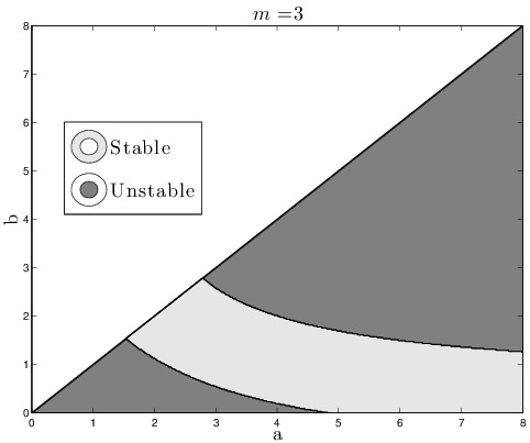
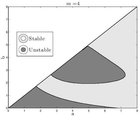
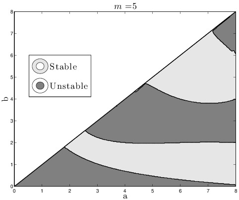
In Figure 2 we recover some results on the stability already shown in [25] . Since I1(m)subscript𝐼1𝑚I_{1}(m) and I2(m)subscript𝐼2𝑚I_{2}(m) depend on the powers a𝑎a and b𝑏b of the power law potential, we plot in the parameter region {(a,b):a>b>0}conditional-set𝑎𝑏𝑎𝑏0\{(a,b)\,:\,a>b>0\} the stability and instability regions depending on the determinant of M𝑀M and its trace. We show the cases m=3,4,5𝑚345m=3,4,5 for a fixed N=100000𝑁100000N=100000.

Refer to caption
Refer to caption
Refer to caption
Figure 2. Stability regions for different perturbations modes m=3,4,5𝑚345m=3,4,5. Stability regions correspond to a couple (a,b)𝑎𝑏(a,b) of parameters where D(a,b)>0,T(a,b)<0formulae-sequence𝐷𝑎𝑏0𝑇𝑎𝑏0D(a,b)>0,\quad T(a,b)<0.

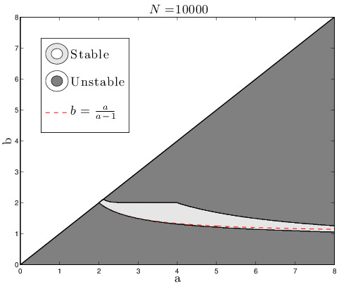
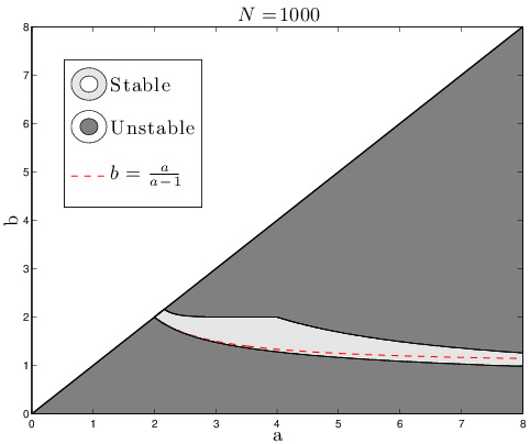
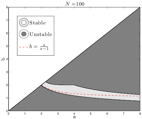
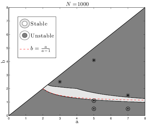
In Figure 3 we compute the stability area as a function of a𝑎a and b𝑏b. To do so, we compute the intersection of all stability areas for m2𝑚2m\geq 2. It can be observed from our tests that the stability area shrinks when the number of particles increases. Moreover, it is observed that in the limit when N𝑁N\to\infty, the lower boundary of the stability region converges to the dashed line. The red dashed line is the curve b=aa1𝑏𝑎𝑎1b=\frac{a}{a-1} that corresponds to the m=+𝑚m=+\infty mode. This curve is the separatrix of the ins/stability regions for the continuous delta ring of the first order continuum model, studied in [25, 3].
Refer to caption
Refer to caption
Refer to caption
Figure 3. Stability areas for flock ring solutions for different values of N𝑁N. From left to right: N=100,1000,10000𝑁100100010000N=100,1000,10000. Markers ()(\bigast) and ()direct-product(\odot) indicate the explored parameters respectively in Table 1 and Table 2.

3.2.1. Cluster formation

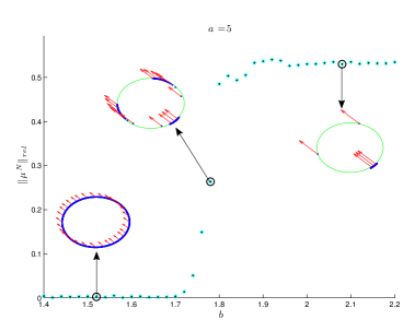
The formation of clusters occurs when the repulsion strength is small. In other words, this phenomenon depends on how singular the potential is at the origin. We show the bifurcation diagram for the phase transition between equally distributed flock and flock with cluster formation.
Refer to caption
Figure 4. Bifurcation diagram for cluster formation at Tf=500subscript𝑇𝑓500T_{f}=500, with N=1000𝑁1000N=1000 particles, a=5𝑎5a=5, |u0|=2.5subscript𝑢02.5|u_{0}|=2.5.

Figure 4 is performed using N=1000𝑁1000N=1000 particles equally distributed on the stable circle with all the velocities aligned. We let them evolve until Tf=500subscript𝑇𝑓500T_{f}=500. We fix the parameters |u0|=2.5subscript𝑢02.5\left|u_{0}\right|=2.5, a=5𝑎5a=5 and vary b𝑏b along the axis. The vertical axis represents the increment of the relative errors

μNrel=μNμ0N2μ0N2subscriptnormsuperscript𝜇𝑁𝑟𝑒𝑙subscriptnormsuperscript𝜇𝑁subscriptsuperscript𝜇𝑁02subscriptnormsubscriptsuperscript𝜇𝑁02\|\mu^{N}\|_{rel}=\frac{\|\mu^{N}-\mu^{N}_{0}\|_{2}}{\|\mu^{N}_{0}\|_{2}}

with increasing b𝑏b, where μ0Nsuperscriptsubscript𝜇0𝑁\mu_{0}^{N} is the uniform distribution along the stable ring of N𝑁N particles and μNsuperscript𝜇𝑁\mu^{N} the distribution at time Tfsubscript𝑇𝑓T_{f}. Simulations are performed with MATLAB and the evolution of the system of odes is solved with the ode45 routine with adaptive time step. Table 1 illustrates different possible final states for different choices of the parameters a,b𝑎𝑏a,b.

a=3,b=2.5formulae-sequence𝑎3𝑏2.5a=3,b=2.5 a=5,b=4.1formulae-sequence𝑎5𝑏4.1a=5,b=4.1 a=7,b=1.5formulae-sequence𝑎7𝑏1.5a=7,b=1.5
[Uncaptioned image] [Uncaptioned image] [Uncaptioned image]
Table 1. Long time simulations with N=1000𝑁1000N=1000 particles. The location of parameter values are marked as ()(\bigast) points in the central plot of Figure 3.

3.2.2. Fattening formation

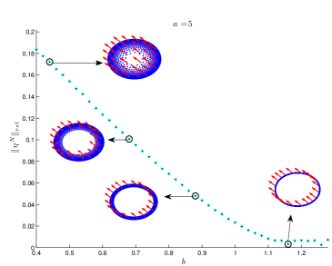
We show the transition diagram between a flock on a ring and a flock on an annulus. In this case, the fattening phenomenon occurs when the parameters of the potential cross the lower boundary of the stability region. We numerically characterize this behavior in a similar way as in the previous subsection.
Refer to caption
Figure 5. Bifurcation diagram for fattening instability at Tf=500subscript𝑇𝑓500T_{f}=500 with N=1000 particles, a=5𝑎5a=5, |u0|=2.5subscript𝑢02.5|u_{0}|=2.5.

Figure 5 is performed using N=1000𝑁1000N=1000 particles equally distributed on the stable ring already in the steady state with all the velocities aligned. We then let them evolve until Tf=500subscript𝑇𝑓500T_{f}=500. We fix the parameters |u0|=2.5subscript𝑢02.5\left|u_{0}\right|=2.5, a=5𝑎5a=5 and vary b𝑏b along the axis. The vertical axis represents the increment of the relative errors

ηNrel=ηNη0N2η0N2subscriptnormsuperscript𝜂𝑁𝑟𝑒𝑙subscriptnormsuperscript𝜂𝑁subscriptsuperscript𝜂𝑁02subscriptnormsubscriptsuperscript𝜂𝑁02\|\eta^{N}\|_{rel}=\frac{\|\eta^{N}-\eta^{N}_{0}\|_{2}}{\|\eta^{N}_{0}\|_{2}}

for increasing b𝑏b, where η0Nsuperscriptsubscript𝜂0𝑁\eta_{0}^{N} represents the average distance from the center of mass for N𝑁N particles in a flock ring formation, i.e., η0N=Rsuperscriptsubscript𝜂0𝑁𝑅\eta_{0}^{N}=R and ηNsuperscript𝜂𝑁\eta^{N} is the average distance from the center of mass at time Tfsubscript𝑇𝑓T_{f}. Table 2 shows the final states for some particular choices of parameters after stabilization.

a=5,b=1.1formulae-sequence𝑎5𝑏1.1a=5,b=1.1 a=5,b=0.5formulae-sequence𝑎5𝑏0.5a=5,b=0.5 a=7,b=0.5formulae-sequence𝑎7𝑏0.5a=7,b=0.5
[Uncaptioned image] [Uncaptioned image] [Uncaptioned image]
Table 2. Long time simulations with N=1000𝑁1000N=1000 particles. The location of parameter values are marked as ()direct-product(\odot) points in the central plot of Figure 3.

3.3. Stability of flock solutions with the Cucker-Smale alignment term

As in Section 3.1 we perform a study on the flock stability for model (3). If we use the same change of variables as in (11), then system (3) reads

{y˙j=vju0=zjz˙j=1Nl=1NH(|ylyj|)(zlzj)+1Nl=1ljNW(ylyj),j=1,,Nformulae-sequencecasessubscript˙𝑦𝑗subscript𝑣𝑗subscript𝑢0subscript𝑧𝑗otherwisesubscript˙𝑧𝑗1𝑁superscriptsubscript𝑙1𝑁𝐻subscript𝑦𝑙subscript𝑦𝑗subscript𝑧𝑙subscript𝑧𝑗1𝑁superscriptsubscript𝑙1𝑙𝑗𝑁𝑊subscript𝑦𝑙subscript𝑦𝑗otherwise𝑗1𝑁\begin{cases}\displaystyle\dot{y}_{j}=v_{j}-u_{0}=z_{j}\\ \displaystyle\dot{z}_{j}=\frac{1}{N}\sum_{l=1}^{N}H(\left|y_{l}-y_{j}\right|)(z_{l}-z_{j})+\frac{1}{N}\sum_{\begin{subarray}{c}l=1\\ l\neq j\end{subarray}}^{N}\nabla W(y_{l}-y_{j})\end{cases},\qquad\qquad\quad j=1,\dots,N (21)

We give a characterization of the flock solution in the complex plane for (21) with (yj0,zj0)=(Reiθj,0),superscriptsubscript𝑦𝑗0superscriptsubscript𝑧𝑗0𝑅superscript𝑒𝑖subscript𝜃𝑗0(y_{j}^{0},z_{j}^{0})=(Re^{i\theta_{j}},0), where θj=2πjNsubscript𝜃𝑗2𝜋𝑗𝑁\theta_{j}=\frac{2\pi j}{N}. We consider then the perturbed solution

y~j(t)=Reiθj(1+hj(t)),subscript~𝑦𝑗𝑡𝑅superscript𝑒𝑖subscript𝜃𝑗1subscript𝑗𝑡\tilde{y}_{j}(t)=Re^{i\theta_{j}}(1+h_{j}(t)),\qquad

with hjsubscript𝑗h_{j} such that |hj|1much-less-thansubscript𝑗1|h_{j}|\ll 1 and satisfying (12). Considering the following relations

y~ly~j=Reiθj(eϕphlhj),subscript~𝑦𝑙subscript~𝑦𝑗𝑅superscript𝑒𝑖subscript𝜃𝑗superscript𝑒subscriptitalic-ϕ𝑝subscript𝑙subscript𝑗\displaystyle\tilde{y}_{l}-\tilde{y}_{j}=Re^{i\theta_{j}}\left(e^{\phi_{p}}h_{l}-h_{j}\right),
|y~ly~j|2R|sin(ϕp2)|+R4|sin(ϕp2)|[(1eiϕp)(hlhj¯)+(1eiϕp)(hl¯hj)],similar-to-or-equalssubscript~𝑦𝑙subscript~𝑦𝑗2𝑅subscriptitalic-ϕ𝑝2𝑅4subscriptitalic-ϕ𝑝2delimited-[]1superscript𝑒𝑖subscriptitalic-ϕ𝑝subscript𝑙¯subscript𝑗1superscript𝑒𝑖subscriptitalic-ϕ𝑝¯subscript𝑙subscript𝑗\displaystyle|\tilde{y}_{l}-\tilde{y}_{j}|\simeq 2R\left|\sin\left(\frac{\phi_{p}}{2}\right)\right|+\frac{R}{4\left|\sin\left(\frac{\phi_{p}}{2}\right)\right|}\left[\left(1-e^{i\phi_{p}}\right)\left(h_{l}-\overline{h_{j}}\right)+\left(1-e^{-i\phi_{p}}\right)\left(\overline{h_{l}}-{h_{j}}\right)\right],
z~lz~j=Reiθj(eϕphlhj),subscript~𝑧𝑙subscript~𝑧𝑗𝑅superscript𝑒𝑖subscript𝜃𝑗superscript𝑒subscriptitalic-ϕ𝑝subscriptsuperscript𝑙subscriptsuperscript𝑗\displaystyle\tilde{z}_{l}-\tilde{z}_{j}=Re^{i\theta_{j}}\left(e^{\phi_{p}}h^{\prime}_{l}-h^{\prime}_{j}\right),

where ϕp=2π(lj)/N=2πp/Nsubscriptitalic-ϕ𝑝2𝜋𝑙𝑗𝑁2𝜋𝑝𝑁\phi_{p}=2\pi(l-j)/N=2\pi p/N. We linearize the Cucker-Smale alignment term around the solution up to first order, leading to

H(|y~ly~j|)similar-to-or-equals𝐻subscript~𝑦𝑙subscript~𝑦𝑗absent\displaystyle H(|\tilde{y}_{l}-\tilde{y}_{j}|)\simeq H(2R|sin(ϕp/2)|)𝐻2𝑅subscriptitalic-ϕ𝑝2\displaystyle H(2R\left|\sin\left(\phi_{p}/2\right)\right|)
+H(2R|sin(ϕp/2)|)R4|sin(ϕp2)|[(1eiϕp)(hlhj¯)+(1eiϕp)(hl¯hj)].superscript𝐻2𝑅subscriptitalic-ϕ𝑝2𝑅4subscriptitalic-ϕ𝑝2delimited-[]1superscript𝑒𝑖subscriptitalic-ϕ𝑝subscript𝑙¯subscript𝑗1superscript𝑒𝑖subscriptitalic-ϕ𝑝¯subscript𝑙subscript𝑗\displaystyle+H^{\prime}(2R\left|\sin\left(\phi_{p}/2\right)\right|)\frac{R}{4\left|\sin\left(\frac{\phi_{p}}{2}\right)\right|}\left[\left(1-e^{i\phi_{p}}\right)\left(h_{l}-\overline{h_{j}}\right)+\left(1-e^{-i\phi_{p}}\right)\left(\overline{h_{l}}-{h_{j}}\right)\right].

Substituting the linearization in (21) and neglecting the second order terms, we obtain the following characterization of hj′′superscriptsubscript𝑗′′h_{j}^{\prime\prime}

hj′′=superscriptsubscript𝑗′′absent\displaystyle h_{j}^{\prime\prime}= 1Nl=1NH(2R|sinϕp|)[eiϕphlhj]1𝑁superscriptsubscript𝑙1𝑁𝐻2𝑅subscriptitalic-ϕ𝑝delimited-[]superscript𝑒𝑖subscriptitalic-ϕ𝑝subscriptsuperscript𝑙subscriptsuperscript𝑗\displaystyle\frac{1}{N}\sum_{l=1}^{N}H(2R|\sin\phi_{p}|)\left[e^{i\phi_{p}}h^{\prime}_{l}-h^{\prime}_{j}\right]
+1Nl=1ljN[G1(ϕp/2)(hjeiϕphl)+G2(ϕp/2)(hl¯eiϕphj¯)].1𝑁superscriptsubscript𝑙1𝑙𝑗𝑁delimited-[]subscript𝐺1subscriptitalic-ϕ𝑝2subscript𝑗superscript𝑒𝑖subscriptitalic-ϕ𝑝subscript𝑙subscript𝐺2subscriptitalic-ϕ𝑝2¯subscript𝑙superscript𝑒𝑖subscriptitalic-ϕ𝑝¯subscript𝑗\displaystyle+\frac{1}{N}\sum_{\begin{subarray}{c}l=1\\ l\neq j\end{subarray}}^{N}\left[G_{1}(\phi_{p}/2)(h_{j}-e^{i\phi_{p}}h_{l})+G_{2}(\phi_{p}/2)(\overline{h_{l}}-e^{i\phi_{p}}\overline{h_{j}})\right]. (22)

In order to study the behavior of the perturbations hjsubscript𝑗h_{j}, we reduce the complexity of the problem, assuming that hjsubscript𝑗h_{j} satisfies the following relation

hj=ξ+(t)eimθj+ξ(t)eimθj,hj=ξ+(t)eimθj+ξ(t)eimθj,m.formulae-sequencesubscript𝑗subscript𝜉𝑡superscript𝑒𝑖𝑚subscript𝜃𝑗subscript𝜉𝑡superscript𝑒𝑖𝑚subscript𝜃𝑗formulae-sequencesubscriptsuperscript𝑗subscriptsuperscript𝜉𝑡superscript𝑒𝑖𝑚subscript𝜃𝑗subscriptsuperscript𝜉𝑡superscript𝑒𝑖𝑚subscript𝜃𝑗𝑚h_{j}=\xi_{+}(t)e^{im\theta_{j}}+\xi_{-}(t)e^{-im\theta_{j}},\quad h^{\prime}_{j}=\xi^{\prime}_{+}(t)e^{im\theta_{j}}+\xi^{\prime}_{-}(t)e^{-im\theta_{j}},\qquad m\in\mathbb{N}.

Therefore, we can express hlsubscript𝑙h_{l} in terms of hjsubscript𝑗h_{j} as

hl=ξ+(t)eimθjeimϕp+ξ(t)eimθjeimϕp,m.formulae-sequencesubscript𝑙subscript𝜉𝑡superscript𝑒𝑖𝑚subscript𝜃𝑗superscript𝑒𝑖𝑚subscriptitalic-ϕ𝑝subscript𝜉𝑡superscript𝑒𝑖𝑚subscript𝜃𝑗superscript𝑒𝑖𝑚subscriptitalic-ϕ𝑝𝑚h_{l}=\xi_{+}(t)e^{im\theta_{j}}e^{im\phi_{p}}+\xi_{-}(t)e^{-im\theta_{j}}e^{-im\phi_{p}},\qquad m\in\mathbb{N}.

Inserting the previous expressions in (22) and gathering terms in eiθjmsuperscript𝑒𝑖subscript𝜃𝑗𝑚e^{i\theta_{j}m} and eiθjmsuperscript𝑒𝑖subscript𝜃𝑗𝑚e^{-i\theta_{j}m}, we can characterize ξ+subscript𝜉\xi_{+} and ξsubscript𝜉\xi_{-} as

ξ+′′=superscriptsubscript𝜉′′absent\displaystyle\xi_{+}^{\prime\prime}= 1Nl=1NH(2R|sinϕp|)[eiϕp(m+1)1]ξ++I1(m)ξ++I2(m)ξ¯,1𝑁superscriptsubscript𝑙1𝑁𝐻2𝑅subscriptitalic-ϕ𝑝delimited-[]superscript𝑒𝑖subscriptitalic-ϕ𝑝𝑚11subscriptsuperscript𝜉subscript𝐼1𝑚subscript𝜉subscript𝐼2𝑚subscript¯𝜉\displaystyle\frac{1}{N}\sum_{l=1}^{N}H(2R|\sin\phi_{p}|)\left[e^{i\phi_{p}(m+1)}-1\right]\xi^{\prime}_{+}+I_{1}(m)\xi_{+}+I_{2}(m)\overline{\xi}_{-},
ξ¯′′=superscriptsubscript¯𝜉′′absent\displaystyle\overline{\xi}_{-}^{\prime\prime}= 1Nl=1NH(2R|sinϕp|)[eiϕp(m1)1]ξ¯+I2(m)ξ++I1(m)ξ¯,1𝑁superscriptsubscript𝑙1𝑁𝐻2𝑅subscriptitalic-ϕ𝑝delimited-[]superscript𝑒𝑖subscriptitalic-ϕ𝑝𝑚11subscript¯𝜉subscript𝐼2𝑚subscript𝜉subscript𝐼1𝑚subscript¯𝜉\displaystyle\frac{1}{N}\sum_{l=1}^{N}H(2R|\sin\phi_{p}|)\left[e^{i\phi_{p}(m-1)}-1\right]\overline{\xi}_{-}+I_{2}(m)\xi_{+}+I_{1}(-m)\overline{\xi}_{-},

where I1subscript𝐼1I_{1} and I2subscript𝐼2I_{2} are defined in (14) and (15). Through a simple manipulation of the sum for the linearized Cucker-Smale term, we obtain that the expression

1NljH(2R|sinϕp|)[eiϕp(m±1)1]=1NljH(2R|sinϕp|)[cos(ϕp(m±1))1]+iNljH(2R|sinϕp|)sin(ϕp(m±1)),1𝑁subscript𝑙𝑗𝐻2𝑅subscriptitalic-ϕ𝑝delimited-[]superscript𝑒𝑖subscriptitalic-ϕ𝑝plus-or-minus𝑚111𝑁subscript𝑙𝑗𝐻2𝑅subscriptitalic-ϕ𝑝delimited-[]subscriptitalic-ϕ𝑝plus-or-minus𝑚11𝑖𝑁subscript𝑙𝑗𝐻2𝑅subscriptitalic-ϕ𝑝subscriptitalic-ϕ𝑝plus-or-minus𝑚1\frac{1}{N}\sum_{l\neq j}H(2R|\sin\phi_{p}|)\left[e^{i\phi_{p}(m\pm 1)}-1\right]=\\ \frac{1}{N}\sum_{l\neq j}H(2R|\sin\phi_{p}|)\left[\cos(\phi_{p}(m\pm 1))-1\right]+\frac{i}{N}\sum_{l\neq j}H(2R|\sin\phi_{p}|)\sin(\phi_{p}(m\pm 1)),

is real. Actually, H(2R|sinϕp|)𝐻2𝑅subscriptitalic-ϕ𝑝H(2R|\sin\phi_{p}|) and sin(ϕp(m±1))subscriptitalic-ϕ𝑝plus-or-minus𝑚1\sin(\phi_{p}(m\pm 1)) are respectively symmetric and antisymmetric with respect to the values of ϕpsubscriptitalic-ϕ𝑝\phi_{p}, so the imaginary part vanishes. Recalling the definition of ϕpsubscriptitalic-ϕ𝑝\phi_{p}, we conclude

J±(m)=subscript𝐽plus-or-minus𝑚absent\displaystyle J_{\pm}(m)= 1Nk=1NH(2R|sin(2πpN)|)[cos(2πpN(m±1))1]1𝑁superscriptsubscript𝑘1𝑁𝐻2𝑅2𝜋𝑝𝑁delimited-[]2𝜋𝑝𝑁plus-or-minus𝑚11\displaystyle\frac{1}{N}\sum_{k=1}^{N}H\left(2R\left|\sin\left(\frac{2\pi p}{N}\right)\right|\right)\left[\cos\left(\frac{2\pi p}{N}(m\pm 1)\right)-1\right]
=\displaystyle= 4Nk=1N/2H(2R|sin(2πpN)|)[sin2(πpN(m±1))].4𝑁superscriptsubscript𝑘1𝑁2𝐻2𝑅2𝜋𝑝𝑁delimited-[]superscript2𝜋𝑝𝑁plus-or-minus𝑚1\displaystyle-\frac{4}{N}\sum_{k=1}^{N/2}H\left(2R\left|\sin\left(\frac{2\pi p}{N}\right)\right|\right)\left[\sin^{2}\left(\frac{\pi p}{N}(m\pm 1)\right)\right].

Therefore, we reduce the stability analysis to the following system

(ξ+′′ξ¯′′)=(I1(m)I2(m)I2(m)I1(m))M(ξ+ξ¯)+(J+(m)00J(m))J(ξ+ξ¯).matrixsuperscriptsubscript𝜉′′missing-subexpressionsuperscriptsubscript¯𝜉′′subscriptmatrixsubscript𝐼1𝑚subscript𝐼2𝑚missing-subexpressionsubscript𝐼2𝑚subscript𝐼1𝑚𝑀matrixsubscript𝜉missing-subexpressionsubscript¯𝜉subscriptmatrixsubscript𝐽𝑚0missing-subexpression0subscript𝐽𝑚𝐽matrixsubscriptsuperscript𝜉missing-subexpression¯subscriptsuperscript𝜉\begin{pmatrix}\xi_{+}^{\prime\prime}\\ \\ \overline{\xi}_{-}^{\prime\prime}\end{pmatrix}=\underbrace{\begin{pmatrix}I_{1}(m)&I_{2}(m)\\ \\ I_{2}(m)&I_{1}(-m)\end{pmatrix}}_{M}\begin{pmatrix}\xi_{+}\\ \\ \overline{\xi}_{-}\end{pmatrix}+\underbrace{\begin{pmatrix}J_{+}(m)&0\\ \\ 0&J_{-}(m)\end{pmatrix}}_{J}\begin{pmatrix}\xi^{\prime}_{+}\\ \\ \bar{\xi^{\prime}_{-}}\end{pmatrix}.

Taking the conjugate in the second equation and relabeling ξ¯subscript¯𝜉\overline{\xi}_{-} with ξsubscript𝜉{\xi}_{-} as in [6], the previous system is equivalent to

ddt(ξ+ξη+η)=(00100001I1(m)I2(m)J+(m)0I2(m)I1(m)0J(m))(ξ+ξη+η)=(0IdMJ)(ξ+ξη+η),𝑑𝑑𝑡matrixsubscript𝜉subscript𝜉subscript𝜂subscript𝜂matrix00100001subscript𝐼1𝑚subscript𝐼2𝑚subscript𝐽𝑚0subscript𝐼2𝑚subscript𝐼1𝑚0subscript𝐽𝑚matrixsubscript𝜉subscript𝜉subscript𝜂subscript𝜂matrix0Id𝑀𝐽matrixsubscript𝜉subscript𝜉subscript𝜂subscript𝜂\frac{d}{dt}\begin{pmatrix}\xi_{+}\\ {\xi}_{-}\\ \eta_{+}\\ {\eta}_{-}\end{pmatrix}=\begin{pmatrix}0&0&1&0\\ 0&0&0&1\\ I_{1}(m)&I_{2}(m)&J_{+}(m)&0\\ I_{2}(m)&I_{1}(-m)&0&J_{-}(m)\\ \end{pmatrix}\begin{pmatrix}\xi_{+}\\ {\xi}_{-}\\ \eta_{+}\\ {\eta}_{-}\end{pmatrix}=\begin{pmatrix}0&\mathrm{Id}\\ M&J\end{pmatrix}\begin{pmatrix}\xi_{+}\\ {\xi}_{-}\\ \eta_{+}\\ {\eta}_{-}\end{pmatrix}, (23)

where η±=ξ±subscript𝜂plus-or-minussubscriptsuperscript𝜉plus-or-minus\eta_{\pm}=\xi^{\prime}_{\pm}.

At this point, we will do a stability analysis based on the eigenvalues of the matrix of the previous system in a similar way as in Section 3.1. If instead of the self-propelled/ friction term we use a Cucker-Smale type alignment term

l=1Ng(|xjxl|)(vjvl),subscriptsuperscript𝑁𝑙1𝑔subscript𝑥𝑗subscript𝑥𝑙subscript𝑣𝑗subscript𝑣𝑙-\sum^{N}_{l=1}g\left(|x_{j}-x_{l}|\right)(v_{j}-v_{l}),

where g(r)𝑔𝑟g(r) denotes any strictly positive function, the corresponding stability matrix LCSsubscript𝐿CSL_{{\rm CS}} for the flock reads

LCS=(0Id𝐌G).subscript𝐿CSmatrix0Id𝐌𝐺L_{{\rm CS}}=\begin{pmatrix}0&\mathrm{Id}\\ \mathbf{M}&-G\end{pmatrix}.

As before, 𝐌𝐌\mathbf{M} denotes stability matrix of the first order model. As the alignment term is linear in the velocity, the matrix G𝐺G acts on 𝐯=(v1,,vN)T,vj2,formulae-sequence𝐯superscriptsubscript𝑣1subscript𝑣𝑁𝑇subscript𝑣𝑗superscript2\mathbf{v}=(v_{1},\ldots,v_{N})^{T},\;v_{j}\in\mathbb{R}^{2}, according to the relation

(G𝐯)j=l=1Ng(|xjxl|)(vjvl).subscript𝐺𝐯𝑗subscriptsuperscript𝑁𝑙1𝑔subscript𝑥𝑗subscript𝑥𝑙subscript𝑣𝑗subscript𝑣𝑙(G\mathbf{v})_{j}=\sum^{N}_{l=1}g\left(|x_{j}-x_{l}|\right)(v_{j}-v_{l}).

In particular, if we denote vjvl22:=(vjvl)(vjvl)assignsubscriptsuperscriptnormsubscript𝑣𝑗subscript𝑣𝑙22superscriptsubscript𝑣𝑗subscript𝑣𝑙subscript𝑣𝑗subscript𝑣𝑙||v_{j}-v_{l}||^{2}_{2}:=(v_{j}-v_{l})^{*}(v_{j}-v_{l}) then this relation implies that

𝐯G𝐯=12j,l=1Ng(|xjxl|)vjvl22.superscript𝐯𝐺𝐯12subscriptsuperscript𝑁𝑗𝑙1𝑔subscript𝑥𝑗subscript𝑥𝑙subscriptsuperscriptnormsubscript𝑣𝑗subscript𝑣𝑙22\mathbf{v}^{*}G\mathbf{v}=\frac{1}{2}\sum^{N}_{j,l=1}g\left(|x_{j}-x_{l}|\right)||v_{j}-v_{l}||^{2}_{2}.

Consequently, G𝐺G is positive semi-definite and G𝐯=𝟎𝐺𝐯0G\mathbf{v}=\mathbf{0} if and only if 𝐯𝐯\mathbf{v} is “constant” in the sense that vjwsubscript𝑣𝑗𝑤v_{j}\equiv w for some fixed w2𝑤superscript2w\in\mathbb{R}^{2}. In other words, ker(G)=span{𝐞1,𝐞2}ker𝐺spansubscript𝐞1subscript𝐞2\mathrm{ker}(G)=\mathrm{span}\left\{\mathbf{e}_{1},\mathbf{e}_{2}\right\}. By translation invariance of the first order model, both 𝐞1ker(𝐌)subscript𝐞1kernel𝐌\mathbf{e}_{1}\in\ker(\mathbf{M}) and 𝐞2ker(𝐌)subscript𝐞2kernel𝐌\mathbf{e}_{2}\in\ker(\mathbf{M}) as well.

Note that the eigenvalue problem for LCSsubscript𝐿CSL_{{\rm CS}} is again equivalent to the following quadratic eigenvalue problem for 𝐱2N𝐱superscript2𝑁\mathbf{x}\in\mathbb{C}^{2N}: λ2𝐱+λG𝐱𝐌𝐱=𝟎superscript𝜆2𝐱𝜆𝐺𝐱𝐌𝐱0\lambda^{2}\mathbf{x}+\lambda G\mathbf{x}-\mathbf{M}\mathbf{x}=\mathbf{0}. Assuming the normalization 𝐱𝐱=1superscript𝐱𝐱1\mathbf{x}^{*}\mathbf{x}=1, the quadratic formula then implies that

λ=𝐱G𝐱±(𝐱G𝐱)2+4𝐱𝐌𝐱2.𝜆plus-or-minussuperscript𝐱𝐺𝐱superscriptsuperscript𝐱𝐺𝐱24superscript𝐱𝐌𝐱2\lambda=\frac{-\mathbf{x}^{*}G\mathbf{x}\pm\sqrt{(\mathbf{x}^{*}G\mathbf{x})^{2}+4\mathbf{x}^{*}\mathbf{M}\mathbf{x}}}{2}.

From this relation and the fact that ker(G)ker(𝐌)ker𝐺ker𝐌\mathrm{ker}(G)\subset\mathrm{ker}(\mathbf{M}) we conclude that ker(LCS)=ker(𝐌)kersubscript𝐿CSker𝐌\mathrm{ker}(L_{{\rm CS}})=\mathrm{ker}(\mathbf{M}), and moreover that (λ)=0λ=0formulae-sequence𝜆0𝜆0\Re(\lambda)=0\quad\Leftrightarrow\quad\lambda=0. Furthermore, 𝐞1subscript𝐞1\mathbf{e}_{1} and 𝐞2subscript𝐞2\mathbf{e}_{2} generate a single generalized eigenvector whereas each remaining 𝐱ker(𝐌)𝐱kernel𝐌\mathbf{x}\in\ker(\mathbf{M}) generates no generalized eigenvectors. Indeed, corresponding to each 𝐱ker(𝐌)𝐱kernel𝐌\mathbf{x}\in\ker(\mathbf{M}) the system of equations

(0Id𝐌G)(𝐮𝐰)=(𝐱𝟎).matrix0Id𝐌𝐺matrix𝐮𝐰matrix𝐱0\begin{pmatrix}0&\mathrm{Id}\\ \mathbf{M}&-G\end{pmatrix}\begin{pmatrix}\mathbf{u}\\ \mathbf{w}\end{pmatrix}=\begin{pmatrix}\mathbf{x}\\ \mathbf{0}\end{pmatrix}.

has a solution if and only if G𝐱=𝟎𝐺𝐱0G\mathbf{x}=\mathbf{0} and 𝐮ker(𝐌)𝐮kernel𝐌\mathbf{u}\in\ker(\mathbf{M}). Additionally, if 𝐱=𝐞i𝐱subscript𝐞𝑖\mathbf{x}=\mathbf{e}_{i} then for any 𝐮ker(𝐌)𝐮kernel𝐌\mathbf{u}\in\ker(\mathbf{M}) the system of equations

(0Id𝐌G)(𝐮~𝐰~)=(𝐮𝐱)matrix0Id𝐌𝐺matrix~𝐮~𝐰matrix𝐮𝐱\begin{pmatrix}0&\mathrm{Id}\\ \mathbf{M}&-G\end{pmatrix}\begin{pmatrix}\tilde{\mathbf{u}}\\ \tilde{\mathbf{w}}\end{pmatrix}=\begin{pmatrix}\mathbf{u}\\ \mathbf{x}\end{pmatrix}

has no solutions. This follows by multiplying the second equation by 𝐱superscript𝐱\mathbf{x}^{*}, then using the facts that 𝐞iker(G)ker(𝐌)subscript𝐞𝑖kernel𝐺kernel𝐌\mathbf{e}_{i}\in\ker(G)\subset\ker(\mathbf{M}) and the facts that G𝐺G and 𝐌𝐌\mathbf{M} are symmetric. In other words, if g(r)𝑔𝑟g(r) is any strictly positive function then

det(LCSλId)=λ2+dim(ker(𝐌))pg(λ),subscript𝐿CS𝜆Idsuperscript𝜆2dimensionkernel𝐌subscript𝑝𝑔𝜆\det(L_{{\rm CS}}-\lambda\mathrm{Id})=\lambda^{2+\dim(\ker(\mathbf{M}))}p_{g}(\lambda),

for some polynomial pg(λ)subscript𝑝𝑔𝜆p_{g}(\lambda) that has non-zero roots. Since this equation holds for any strictly positive function g(r),𝑔𝑟g(r), we may follow the proof of Theorem 1 to conclude that the second order model has an eigenvalue with positive real part if and only if the first order system has a positive eigenvalue. Moreover, the vectors (𝐞i,𝐞i)subscript𝐞𝑖subscript𝐞𝑖(\mathbf{e}_{i},\mathbf{e}_{i}) for each i=1,2𝑖12i=1,2 furnish generalized eigenvectors with eigenvalue zero, so the ring flock is always linearly unstable. As a summary, we have shown:

Theorem 2.

The linearized second order system (3) around the flock ring solution has an eigenvalue with positive real part if and only if the linearized first order system around the ring solution has a positive eigenvalue. As a consequence, the flock ring solution is unstable for m𝑚m-mode perturbations for the second order model (3) if and only if the ring solution is unstable for m𝑚m-mode perturbations for the first order model (2).

The linear stability analysis of the previous system leads to the characterization of the stability areas in Figure 6. We show that the stability parameter regions for different values of N𝑁N, and γ=1𝛾1\gamma=1 coincide with the ones in Figure 3.

Refer to caption
Refer to caption
Refer to caption
Figure 6. Stability regions for flock ring solutions with the Cucker-Smale term for different values of N𝑁N.

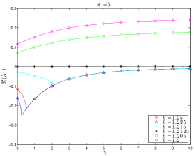
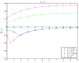
We also investigate the behavior of the eigenvalue with the largest real part, (λ1)subscript𝜆1\Re(\lambda_{1}), of the linearized system (23) against the increasing value of communication strength γ𝛾\gamma. In Figure 7, as the potential gets more repulsive at the origin, we see the change from stability to instability, and the rate of convergence to equilibrium depending on γ𝛾\gamma.

Refer to caption
Refer to caption
Figure 7. The magnitude of (λ1)subscript𝜆1\Re(\lambda_{1}) is influenced by γ𝛾\gamma, for different values of b𝑏b and fixed a=5𝑎5a=5, N=10000𝑁10000N=10000.

4. Stability for mill solutions

This section is devoted to complement the results in [6] by analyzing the stability of mill ring solutions with repulsion.

4.1. Linear stability analysis

Let us consider the transformation

{yj(t)=O(t)xj(t)zj(t)=O(t)vj(t),j=1,,Nformulae-sequencecasessubscript𝑦𝑗𝑡𝑂𝑡subscript𝑥𝑗𝑡otherwisesubscript𝑧𝑗𝑡𝑂𝑡subscript𝑣𝑗𝑡otherwise𝑗1𝑁\begin{cases}y_{j}(t)=O(t)x_{j}(t)\\ z_{j}(t)=O(t)v_{j}(t)\end{cases},\quad j=1,\dots,N

where O(t)𝑂𝑡O(t) is the rotation matrix defined as

O(t)=eSt,S=(0ωω0),andO˙(t)=SeSt.formulae-sequence𝑂𝑡superscript𝑒𝑆𝑡formulae-sequence𝑆matrix0𝜔𝜔0and˙𝑂𝑡𝑆superscript𝑒𝑆𝑡O(t)=e^{St},\quad S=\begin{pmatrix}0&\omega\\ -\omega&0\end{pmatrix},\quad\mbox{and}\quad\dot{O}(t)=Se^{St}.

Evaluating y˙j(t)subscript˙𝑦𝑗𝑡\dot{y}_{j}(t) and z˙j(t)subscript˙𝑧𝑗𝑡\dot{z}_{j}(t) and after some straightforward computations, we get

{y˙j(t)=Syj(t)+zj(t)z˙j(t)=Szj(t)+(αβ|zj|2)zj(t)1Nl=1ljNW(ylyj),j=1,,N.formulae-sequencecasessubscript˙𝑦𝑗𝑡𝑆subscript𝑦𝑗𝑡subscript𝑧𝑗𝑡otherwisesubscript˙𝑧𝑗𝑡𝑆subscript𝑧𝑗𝑡𝛼𝛽superscriptsubscript𝑧𝑗2subscript𝑧𝑗𝑡1𝑁superscriptsubscript𝑙1𝑙𝑗𝑁𝑊subscript𝑦𝑙subscript𝑦𝑗otherwise𝑗1𝑁\begin{cases}\displaystyle\dot{y}_{j}(t)=Sy_{j}(t)+z_{j}(t)\\ \displaystyle\dot{z}_{j}(t)=Sz_{j}(t)+(\alpha-\beta|z_{j}|^{2})z_{j}(t)-\frac{1}{N}\sum_{\begin{subarray}{c}l=1\\ l\neq j\end{subarray}}^{N}\nabla W(y_{l}-y_{j})\end{cases},\quad j=1,\dots,N.

A linear stability analysis for mill rings was performed in [6]. Actually, for a fixed number of particles, we have a mill ring solution given by (yj0,zj0)=(Reiθj,0),superscriptsubscript𝑦𝑗0superscriptsubscript𝑧𝑗0𝑅superscript𝑒𝑖subscript𝜃𝑗0(y_{j}^{0},z_{j}^{0})=(Re^{i\theta_{j}},0), where θj=2πjNsubscript𝜃𝑗2𝜋𝑗𝑁\theta_{j}=\frac{2\pi j}{N}, and R𝑅R determined by equation (7). With the same notation as in Section 3, the analysis in [6] leads to the linear system

(ξ+ξη+η)=(00100001ωiα+ω2+I1(m)ωiα+I2(m)α2ωiαωiα+I2(m)ωiα+ω2+I1(m)αα+2ωi)(ξ+ξη+η).matrixsubscriptsuperscript𝜉subscriptsuperscript𝜉subscriptsuperscript𝜂subscriptsuperscript𝜂matrix00100001𝜔𝑖𝛼superscript𝜔2subscript𝐼1𝑚𝜔𝑖𝛼subscript𝐼2𝑚𝛼2𝜔𝑖𝛼𝜔𝑖𝛼subscript𝐼2𝑚𝜔𝑖𝛼superscript𝜔2subscript𝐼1𝑚𝛼𝛼2𝜔𝑖matrixsubscript𝜉subscript𝜉subscript𝜂subscript𝜂\begin{pmatrix}\xi^{\prime}_{+}\\ {\xi}^{\prime}_{-}\\ \eta^{\prime}_{+}\\ {\eta}^{\prime}_{-}\end{pmatrix}=\begin{pmatrix}0&0&1&0\\ 0&0&0&1\\ -\omega i\alpha+\omega^{2}+I_{1}(m)&-\omega i\alpha+I_{2}(m)&-\alpha-2\omega i&\alpha\\ \omega i\alpha+I_{2}(m)&\omega i\alpha+\omega^{2}+I_{1}(-m)&\alpha&-\alpha+2\omega i\end{pmatrix}\begin{pmatrix}\xi_{+}\\ {\xi}_{-}\\ \eta_{+}\\ {\eta}_{-}\end{pmatrix}. (24)

Let us remind that the perturbations are of the form y~j(t)=Reiθj(1+hj(t))subscript~𝑦𝑗𝑡𝑅superscript𝑒𝑖subscript𝜃𝑗1subscript𝑗𝑡\tilde{y}_{j}(t)=Re^{i\theta_{j}}(1+h_{j}(t)), with hj=ξ+(t)eimθj+ξ(t)eimθjsubscript𝑗subscript𝜉𝑡superscript𝑒𝑖𝑚subscript𝜃𝑗subscript𝜉𝑡superscript𝑒𝑖𝑚subscript𝜃𝑗h_{j}=\xi_{+}(t)e^{im\theta_{j}}+\xi_{-}(t)e^{-im\theta_{j}}, m=2,3,,𝑚23m=2,3,\dots, such that |hj|1much-less-thansubscript𝑗1|h_{j}|\ll 1 and satisfying (12), with (η+,η)=(ξ+,ξ)subscript𝜂subscript𝜂subscriptsuperscript𝜉subscriptsuperscript𝜉(\eta_{+},{\eta}_{-})=(\xi^{\prime}_{+},{\xi}^{\prime}_{-}). We will make use of (24) to study the stability of mill rings with repulsion.

4.2. Numerical tests

Unlike the case of flock solutions where the asymptotic speed does not play role in the linear stability, we will show that the asymptotic speed |u0|subscript𝑢0|u_{0}| can be used as a bifurcation parameter for mills.

In Table 3 we numerically investigate the behavior of the stability region for a fixed number of particles, N=1000𝑁1000N=1000, and for increasing values of the asymptotic speed |u0|subscript𝑢0|u_{0}|. We observe that the stability region shrinks with respect to a𝑎a and gets larger with respect to b𝑏b. Each stability region in Table 3 is computed out of the intersection of the stable areas for the system (24) for each perturbation mode m2𝑚2m\geq 2. Note that for |u0|=0subscript𝑢00|u_{0}|=0 the stability region coincides with the one for the the first order model (2) and for the flock ring solution.

[Uncaptioned image] [Uncaptioned image] [Uncaptioned image]
[Uncaptioned image] [Uncaptioned image] [Uncaptioned image]
Table 3. Stability region for N=1000𝑁1000N=1000 and different values of the asymptotic speed |u0|subscript𝑢0|u_{0}|. Markers ()direct-product(\odot) and ()(\bigast) correspond to the explored parameters in Table 4 and Table 5.

A similar analysis, as done in Subsection 3.2, can be performed to study the formation of fat mills and clustered mill solutions. We show how both the fattening and the clustering instability are triggered by tunning the asymptotic speed for a choice of the interaction potential (a𝑎a and b𝑏b).

In the case of flock ring solutions we observe cluster solutions or annulus solutions when parameters a𝑎a and b𝑏b are chosen respectively “below” or “above” the stability region. In the case of mill solutions, a similar behavior is observed, but this will depend also on the chosen value of |u0|subscript𝑢0|u_{0}|. As an example, we fix (a,b)=(5,0.5)𝑎𝑏50.5(a,b)=(5,0.5), marked as ()direct-product(\odot) in Table 3, and we observe the behavioral change of the system for increasing values of the asymptotic speed.

Table 4 exhibits this switching behavior from a fat mill to a cluster pattern along with the increment of the asymptotic speed. We observe that for small values of the asymptotic speed fat mill solutions are stable patterns, but when increasing the value of |u0|subscript𝑢0\left|u_{0}\right| the stable solutions form a clustered mill. The first row shows the evolution of the system with asymptotic speed |u0|=0.25subscript𝑢00.25\left|u_{0}\right|=0.25 towards an annulus mill. In the second row we take |u0|=0.5subscript𝑢00.5\left|u_{0}\right|=0.5 the previous stable solution is reshaped to a fat clusters pattern. The speed in the third row is switched to |u0|=5subscript𝑢05\left|u_{0}\right|=5 and clusters on lines emerge as a stable configuration. Increasing the speed to |u0|=50subscript𝑢050\left|u_{0}\right|=50 in the fourth row we can observe that clusters on “points” are stable solutions.

|u0|subscript𝑢0\left|u_{0}\right| Stable
0.250.250.25 [Uncaptioned image] [Uncaptioned image] [Uncaptioned image] [Uncaptioned image]
0.50.50.5 [Uncaptioned image] [Uncaptioned image] [Uncaptioned image] [Uncaptioned image]
555 [Uncaptioned image] [Uncaptioned image] [Uncaptioned image] [Uncaptioned image]
505050 [Uncaptioned image] [Uncaptioned image] [Uncaptioned image] [Uncaptioned image]
Table 4. N=1000𝑁1000N=1000 particles, a=5,b=0.5formulae-sequence𝑎5𝑏0.5a=5,b=0.5. The table shows the evolution of a mill ring for increasing values of the speed |u0|subscript𝑢0\left|u_{0}\right|. Each row depicts the behavior of the system for a fixed speed, until a stable state is reached. The evolution of the second, third and fourth row is computed starting from the stable pattern of the previous line.

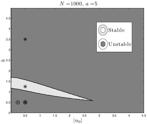
In Figure 8 we numerically show how the stability region looks like in terms of (|u0|,b)subscript𝑢0𝑏(|u_{0}|,b), with a𝑎a fixed at 0.50.50.5, and we enlighten with marker points ()direct-product(\odot) the parameter choices of Table 4, first and second lines.

For the sake of completeness, we enrich the analysis fixing |u0|=0.5subscript𝑢00.5\left|u_{0}\right|=0.5 and considering different values of b𝑏b, in order to cross the stability region. Therefore in Table 5 we show the evolution of a mill ring solution with b𝑏b taken subsequently equal to 0.5,1.25,3.50.51.253.50.5,1.25,3.5, parameter choices are marked as (\bigast) in Figure 8. The first line of Table 5 shows the convergence to the same stable state as the one in second line of Table 4, but, since the system starts to evolve directly from a ring mill solution, the transient behavior is different. Parameters in second line belong to the stability region, see Figure 8. Therefore, the stable state becomes a mill ring solution. Finally, in the third line we increase b𝑏b and a three point cluster solution is observed as stable pattern.

b𝑏b Stable
0.50.50.5 [Uncaptioned image] [Uncaptioned image] [Uncaptioned image] [Uncaptioned image]
1.251.251.25 [Uncaptioned image] [Uncaptioned image] [Uncaptioned image] [Uncaptioned image]
3.53.53.5 [Uncaptioned image] [Uncaptioned image] [Uncaptioned image] [Uncaptioned image]
Table 5. N=1000𝑁1000N=1000 particles, a=5,|u0|=0.5formulae-sequence𝑎5subscript𝑢00.5a=5,|u_{0}|=0.5. The table shows the evolution of a mill ring for increasing values of b𝑏b, i.e. decreasing repulsion. The evolution of the second and the third row is computed starting from the stable pattern of the previous line.
Refer to caption
Figure 8. Stability region for mill ring solution with parameter a=5𝑎5a=5, N=1000𝑁1000N=1000. Markers ()direct-product(\odot) and ()(\bigast) depict the parameter choices respectively for Table 4 and Table 5.

4.2.1. Mill to Flock and Flock to Mill behavior

We numerically investigate the stability of mill and flock ring solutions for small values of the asymptotic speed, |u0|subscript𝑢0|u_{0}|, and the parameter b𝑏b, which corresponds to a strong repulsion condition.

We perform two representative simulations showing that for a particular choice of the parameters, mill ring solutions can switch to fat flock solutions and conversely flock mill solutions switch to fat mill patterns.

[Uncaptioned image] [Uncaptioned image] [Uncaptioned image] [Uncaptioned image]
[Uncaptioned image] [Uncaptioned image] [Uncaptioned image] [Uncaptioned image]
Table 6. System with N=100𝑁100N=100 agents, parameters are fixed a=4𝑎4a=4 and b=0.0005𝑏0.0005b=0.0005 and |u0|=0.01subscript𝑢00.01|u_{0}|=0.01. The first row shows that the initial mill ring configuration is unstable. The second row outlines the self organization of the system in a fat flock configuration.

In Table 6 we take N=100𝑁100N=100 particles and we fix a=4,b=0.0005formulae-sequence𝑎4𝑏0.0005a=4,b=0.0005 and |u0|=0.01subscript𝑢00.01|u_{0}|=0.01. The frames in the first row show the instability of mill ring solutions for this choice of parameters. The system initially evolves to an almost chaotic state, then particles start to organize rotating around the center of mass. This rotation actually causes the alignment of the agents and the final fat flock configuration described in the second row. In Table 7 we consider as initial state a flock ring solution. The parameters of the model are N=100𝑁100N=100, a=4𝑎4a=4, b=0.001𝑏0.001b=0.001 and |u0|=0.1subscript𝑢00.1|u_{0}|=0.1. The first row of the table illustrates that the initial configuration is not a stable solution. Therefore, the symmetry of the flock ring is broken and the system exhibits a chaotic behavior. In the second row a rotating dynamic emerges out of the disordered state and finally the system stabilizes to a fat mill solution.

[Uncaptioned image] [Uncaptioned image] [Uncaptioned image] [Uncaptioned image]
[Uncaptioned image] [Uncaptioned image] [Uncaptioned image] [Uncaptioned image]
Table 7. System with N=100𝑁100N=100 agents, parameters a=4𝑎4a=4 and b=0.001𝑏0.001b=0.001 and |u0|=0.1subscript𝑢00.1|u_{0}|=0.1. The first row shows the instability of the flock ring solution while the second exhibits the convergence to a fat mill type solution.

These numerical tests show surprisingly that it is possible, with a particular choice of the parameters, to obtain mill configurations out of perturbations of initial flock solutions and flock solutions out of perturbations of mill ring solutions. These heteroclinic-kind solutions have not been previously reported. We also remark that the parameter choice is connected to the number of agents we are considering; changing N𝑁N means finding another set of parameters for which the same switching behavior occurs.

References

  • [1] I. Aoki. A simulation study on the schooling mechanism in fish. Bull. Japan Soc. Sci. Fish, 48:1081–1088, 1982.
  • [2] D. Balagué, J. A. Carrillo, T. Laurent, and G. Raoul. Dimensionality of local minimizers of the interaction energy. to appear in ARMA, 2013.
  • [3] D. Balagué, J. A. Carrillo, T. Laurent, and G. Raoul. Nonlocal interactions by repulsive-attractive potentials: radial ins/stability. to appear in Physica D, 2013.
  • [4] M. Ballerini, N. Cabibbo, R. Candelier, A. Cavagna, E. Cisbani, I. Giardina, V. Lecomte, A. Orlandi, G. Parisi, A. Procaccini, M. Viale, and V. Zdravkovic. Interaction ruling animal collective behavior depends on topological rather than metric distance: Evidence from a field study. Proceedings of the National Academy of Sciences, 105(4):1232–1237, 2008.
  • [5] A. B. T. Barbaro, K. Taylor, P. F. Trethewey, L. Youseff, and B. Birnir. Discrete and continuous models of the dynamics of pelagic fish: application to the capelin. Math. Comput. Simulation, 79(12):3397–3414, 2009.
  • [6] A. L. Bertozzi, H. Sun, J. von Brecht, T. Kolokolnikov, and D. Uminsky. Ring patterns and their bifurcations in the model of biological swarms. Submitted.
  • [7] B. Birnir. An ODE model of the motion of pelagic fish. J. Stat. Phys., 128(1 - 2):535–568, 2007.
  • [8] S. Camazine, J.L. Deneubourg, N. R. Franks, J. Sneyd, G. Theraulaz, and E. Bonabeau. Self-Organization in Biological Systems. Princeton University Press, Princeton, 2001.
  • [9] J. A. Cañizo, J. A. Carrillo, and J. Rosado. A well-posedness theory in measures for some kinetic models of collective motion. Math. Models Methods Appl. Sci., 21(3):515–539, 2011.
  • [10] J. A. Carrillo, M. Fornasier, J. Rosado, and G. Toscani. Asymptotic flocking dynamics for the kinetic cucker-smale model. SIAM J. Math. Anal., 42:218–236, 2010.
  • [11] J. A. Carrillo, Y. Huang, and S. Martin. Existence, uniqueness, and orbital stability of localized flock solutions in kinetic models. work in preparation, 2013.
  • [12] J.A. Carrillo, M.R. D’Orsogna, and V. Panferov. Double milling in self-propelled swarms from kinetic theory. Kin. Rel. Mod., 2:363–378, 2009.
  • [13] Y. Chuang, M. R. D’Orsogna, D. Marthaler, and L. Chayes A. Bertozzi. State transitions and the continuum limit for interacting, self-propelled particles. Phys. D, 232:33–47, 2007.
  • [14] F. Cucker and S. Smale. Emergent behavior in flocks. IEEE Trans. Automat. Control, 52(5):852–862, 2007.
  • [15] F. Cucker and S. Smale. On the mathematics of emergence. Jpn. J. Math., 2(1):197–227, 2007.
  • [16] P. Degond and S. Motsch. Continuum limit of self-driven particles with orientation interaction. Math. Models Methods Appl. Sci., 18(suppl.):1193–1215, 2008.
  • [17] M. R. D’Orsogna, Y. Chuang, A. Bertozzi, and L. Chayes. Self-propelled particles with soft-core interactions: patterns, stability and collapse. Phys. Rev. Lett., 96(104302), 2006.
  • [18] A. Dussutour, S.C. Nicolis, J.-L. Deneubourg, and V. Fourcassié. Collective decision in ants under crowded conditions. Behavioral Ecology and Sociobiology, 61(17-30), 2006.
  • [19] S.-Y. Ha and J.-G. Liu. A simple proof of the Cucker-Smale flocking dynamics and mean-field limit. Commun. Math. Sci., 7(2):297–325, 2009.
  • [20] S. Y. Ha and E. Tadmor. From particle to kinetic and hydrodynamic descriptions of flocking. Kinet. Relat. Models, 1(3):415–435, 2008.
  • [21] C. K. Hemelrijk and H. Hildenbrandt. Self-organized shape and frontal density of fish schools. Ethology, 114:245–254, 2008.
  • [22] A. Huth and C. Wissel. The simulation of fish schools in comparison with experimental data. Ecol. Model., 75/76:135–145, 1994.
  • [23] A. L. Koch and D. White. The social lifestyle of myxobacteria. BioEssays, 20(12):1030–1038, 1998.
  • [24] T. Kolokolnikov, Y. Huang, and M. Pavlovski. Singular patterns for an aggregation model with a confining potential. to appear in Physica D.
  • [25] T. Kolokonikov, H. Sun, D. Uminsky, and A. Bertozzi. Stability of ring patterns arising from 2d particle interactions. Physical Review E, 84(1):015203, 2011.
  • [26] H. Levine, W.-J. Rappel, and I. Cohen. Self-organization in systems of self-propelled particles. Phys. Rev. E, 63:017101, Dec 2000.
  • [27] R. Lukeman, Y.X. Li, and L. Edelstein-Keshet. Inferring individual rules from collective behavior. Proc. Natl. Acad. Sci. U.S.A., 107(28):12576–12580, 2010.
  • [28] J. Parrish and L. Edelstein-Keshet. Complexity, pattern, and evolutionary trade-offs in animal aggregation. Science, 284(5411):99 –101, 1999.
  • [29] T. Vicsek, A. Czirók, E. Ben-Jacob, I. Cohen, and O. Shochet. Novel type of phase transition in a system of self-driven particles. Phys. Rev. Lett., 75(6):1226–1229, 1995.
  • [30] J. von Brecht, D. Uminsky, T. Kolokolnikov, and A. Bertozzi. Predicting pattern formation in particle interactions. Math. Mod. Meth. Appl. Sci., 22:1140002, 2012.