Quantum Popov robust stability analysis of an optical cavity containing a saturated Kerr medium

Abstract

This paper applies results on the robust stability of nonlinear quantum systems to a system consisting an optical cavity containing a saturated Kerr medium. The system is characterized by a Hamiltonian operator which contains a non-quadratic term involving a quartic function of the annihilation and creation operators. A saturated version of the Kerr nonlinearity leads to a sector bounded nonlinearity which enables a quantum small gain theorem to be applied to this system in order to analyze its stability. Also, a non-quadratic version of a quantum Popov stability criterion is presented and applied to analyze the stability of this system.

I Introduction

The use of Kerr media is commonly found in applications of nonlinear optics; e.g., see [1, 2]. A Kerr medium is characterized by a refractive index which increases with the intensity of light applied to the medium; e.g., see Section 9.1.1. of [3]. Within the area of quantum optics, a Kerr medium is often characterized by a Hamiltonian operator which is a quartic function of the annihilation and creation operators; e.g., see Section 5.4 of [4]. This leads to a nonlinear quantum stochastic differential equation which contains a cubic nonlinearity [4]. In this paper, we apply some recent and new quantum robust stability analysis tools to analyze the stability of an optical cavity containing a Kerr medium. Such as system has been proposed as a method of generating squeezed light; see Chapter 9 of [3]. Squeezed light is an intrinsically quantum phenomenon which has potential applications in areas such as gravity wave detection, precision metrology and quantum computing [3, 5]. Also note that the quantum dynamics obtained in the case of a microwave resonator containing a Josephson junction can be used to approximate the case of a Kerr medium in a cavity; e.g., see [6]. Such a system is related to the system analyzed in [7].

The first method we will apply to analyze the robust stability of the system under consideration is the quantum small gain result presented in [8]. This result gives a sufficient condition for the robust stability of uncertain nonlinear quantum systems in which the uncertainty is introduced by considering a non-quadratic perturbation to the system Hamiltonian operator. Such a non-quadratic perturbation leads to a nonlinear quantum stochastic differential equation describing the system; e.g., [9]. This nonlinearity is required to satisfy a certain sector bound condition. Related results to the results of [8] can be found in [10, 11] and consider different classes of perturbations. Furthermore, the paper [12] introduces a quantum version of the Popov stability criterion (e.g., see [13] for the classical Popov stability criterion), which allows for quadratic perturbations to the system Hamiltonian. That is, the paper [12] considers uncertain quantum linear systems. In this paper we introduce a new version of the quantum Popov stability criterion which allows for non-quadratic perturbations to the system Hamiltonian and thus nonlinear uncertain quantum systems. As in [8], the nonlinearity is required to satisfy a certain sector bound condition. This result is applied to analyze the system consisting of an optical cavity containing a Kerr medium.

For the quantum robust stability result introduced in [8] and in the new quantum Popov stability result introduced in this paper, the nominal quantum system is assumed to be a quantum linear system; e.g., see [14, 15, 16, 17, 18]. In addition, the nonlinearity is required to satisfy certain sector bound and smoothness conditions. However, for the standard quartic Hamiltonian model of a Kerr medium, the resulting cubic nonlinearity will not satisfy the sector bound conditions for any finite sector. We overcome this difficulty by noting that any practical implementation of a Kerr medium will not be precisely modelled by a quartic Hamiltonian but rather will suffer from some saturation effects; e.g., see [19]. This allows us to model the Kerr medium with a non-quadratic Hamiltonian such that the sector bound and smoothness conditions required in our quantum robust stability analysis results are satisfied.

The remainder of the paper proceeds as follows. In Section II, we define the general class of nonlinear uncertain nonlinear quantum systems under consideration. In this section, we also also recall the main result of [8] and present a new Popov type stability result for this class of nonlinear quantum systems. In Section III, we analyze the system consisting of an optical cavity containing a saturated Kerr nonlinearity using the two quantum robust stability analysis results presented. In Section IV, we present some conclusions. The proofs of all of the main results are given in the Appendix.

II Robust Stability of Uncertain Nonlinear Quantum Systems

In this section, we describe the general class of quantum systems under consideration. As in the papers [9, 20, 8, 10, 12], we consider uncertain nonlinear open quantum systems defined by parameters $(S,L,H)$ where $S$ is the scattering matrix which is typically chosen as the identity matrix, L is the coupling operator and $H$ is the system Hamiltonian operator which is assumed to be of the form

$$H=\frac{1}{2}\left[\begin{array}[]{cc}a^{\dagger}&a^{T}\end{array}\right]M\left[\begin{array}[]{c}a\\ a^{\#}\end{array}\right]+f(z,z^{*}).$$ (1)

Here $a$ is a vector of annihilation operators on the underlying Hilbert space and $a^{\#}$ is the corresponding vector of creation operators. Also, $M\in\mathbb{C}^{2n\times 2n}$ is a Hermitian matrix of the form

$$M=\left[\begin{array}[]{cc}M_{1}&M_{2}\\ M_{2}^{\#}&M_{1}^{\#}\end{array}\right]$$ (2)

and $M_{1}=M_{1}^{\dagger}$, $M_{2}=M_{2}^{T}$. In the case vectors of operators, the notation ^† refers to the transpose of the vector of adjoint operators and in the case of matrices, this notation refers to the complex conjugate transpose of a matrix. In the case vectors of operators, the notation ^# refers to the vector of adjoint operators and in the case of complex matrices, this notation refers to the complex conjugate matrix. Also, the notation ^∗ denotes the adjoint of an operator. The matrix $M$ is assumed to be known and defines the nominal quadratic part of the system Hamiltonian. Furthermore, we assume the uncertain non-quadratic part of the system Hamiltonian $f(z,z^{*})$ is defined by a formal power series of the form

$$f(z,z^{*})=\sum_{k=0}^{\infty}\sum_{\ell=0}^{\infty}S_{k\ell}z^{k}(z^{*})^{\ell},$$ (3)

which is assumed to converge in some suitable sense. Here $S_{k\ell}=S_{\ell k}^{*}$, and $z$ is a known scalar operator defined by

$$z = E_{1}a+E_{2}a^{\#}$$ (9)

$$= \left[\begin{array}[]{cc}E_{1}&E_{2}\end{array}\right]\left[\begin{array}[]{c}a\\ a^{\#}\end{array}\right]=\tilde{E}\left[\begin{array}[]{c}a\\ a^{\#}\end{array}\right].$$

The term $f(z,z^{*})$ is referred to as the perturbation Hamiltonian. It is assumed to be unknown but is contained within a known set which will be defined below. Two different sets of perturbations will be considered depending on the robust stability condition which is to be applied.

We assume the coupling operator $L$ is known and is of the form

$$L=\left[\begin{array}[]{cc}N_{1}&N_{2}\end{array}\right]\left[\begin{array}[]{c}a\\ a^{\#}\end{array}\right]$$ (10)

where $N_{1}\in\mathbb{C}^{m\times n}$ and $N_{2}\in\mathbb{C}^{m\times n}$. Also, we write

$$\left[\begin{array}[]{c}L\\ L^{\#}\end{array}\right]=N\left[\begin{array}[]{c}a\\ a^{\#}\end{array}\right]=\left[\begin{array}[]{cc}N_{1}&N_{2}\\ N_{2}^{\#}&N_{1}^{\#}\end{array}\right]\left[\begin{array}[]{c}a\\ a^{\#}\end{array}\right].$$

The annihilation and creation operators are assumed to satisfy the canonical commutation relations:

$$\left[\left[\begin{array}[]{l}a\\ a^{\#}\end{array}\right],\left[\begin{array}[]{l}a\\ a^{\#}\end{array}\right]^{\dagger}\right] \stackrel{{\scriptstyle\Delta}}{{=}} \left[\begin{array}[]{l}a\\ a^{\#}\end{array}\right]\left[\begin{array}[]{l}a\\ a^{\#}\end{array}\right]^{\dagger}$$ (24)

$$-\left(\left[\begin{array}[]{l}a\\ a^{\#}\end{array}\right]^{\#}\left[\begin{array}[]{l}a\\ a^{\#}\end{array}\right]^{T}\right)^{T}$$

$$= J$$ (25)

where $J=\left[\begin{array}[]{cc}I&0\\ 0&-I\end{array}\right]$; e.g., see [21, 22, 18].

To define the set of allowable perturbation Hamiltonians $f(\cdot)$, we first define the following formal partial derivatives:

$$\frac{\partial f(z,z^{*})}{\partial z}\stackrel{{\scriptstyle\Delta}}{{=}}\sum_{k=1}^{\infty}\sum_{\ell=0}^{\infty}kS_{k\ell}z^{k-1}(z^{*})^{\ell};$$ (26)

$$\frac{\partial^{2}f(z,z^{*})}{\partial z^{2}}\stackrel{{\scriptstyle\Delta}}{{=}}\sum_{k=1}^{\infty}\sum_{\ell=0}^{\infty}k(k-1)S_{k\ell}z^{k-2}(z^{*})^{\ell};$$ (27)

$$\frac{\partial^{2}f(z,z^{*})}{\partial z\partial z^{*}}\stackrel{{\scriptstyle\Delta}}{{=}}\sum_{k=1}^{\infty}\sum_{\ell=1}^{\infty}k\ell S_{k\ell}z^{k-1}(z^{*})^{\ell-1}.$$ (28)

Then for given constants $\gamma>0$, $\beta>0$, $\delta_{1}\geq 0$, $\delta_{2}\geq 0$, $\delta_{3}\geq 0$, we consider the sector bound conditions

$$\frac{\partial f(z,z^{*})}{\partial z}^{*}\frac{\partial f(z,z^{*})}{\partial z}\leq\frac{1}{\gamma^{2}}zz^{*}+\delta_{1};$$ (29)

$$\left(\frac{\partial f(z,z^{*})}{\partial z}-\frac{1}{\gamma}z^{*}\right)^{*}\left(\frac{\partial f(z,z^{*})}{\partial z}-\frac{1}{\gamma}z^{*}\right)$$ (30)

$$\leq \frac{1}{\gamma^{2}}zz^{*}+\delta_{1};\hskip 142.26378pt$$

and the smoothness conditions

$$\frac{\partial^{2}f(z,z^{*})}{\partial z^{2}}^{*}\frac{\partial^{2}f(z,z^{*})}{\partial z^{2}}\leq\delta_{2};$$ (31)

$$\frac{\partial^{2}f(z,z^{*})}{\partial z\partial z^{*}}^{*}\frac{\partial^{2}f(z,z^{*})}{\partial z\partial z^{*}}\leq\delta_{3}.$$ (32)

Also, we consider the following upper and lower bounds on the perturbation Hamiltonian

$$0\leq f(z,z^{*})\leq\beta zz^{*}.$$ (33)

Then we define two possible sets of perturbation Hamiltonians $\mathcal{W}_{1}$ and $\mathcal{W}_{2}$ as follows:

$$\mathcal{W}_{1}=\left\{\begin{array}[]{l}f(\cdot)\mbox{ of the form (\ref{H2nonquad}) such that }\\ \mbox{ conditions (\ref{sector1}) and (\ref{smooth1}) are satisfied}\end{array}\right\};$$ (34)

$$\mathcal{W}_{2}=\left\{\begin{array}[]{l}f(\cdot)\mbox{ of the form (\ref{H2nonquad}) such that }\\ \mbox{ conditions (\ref{sector2}), (\ref{smooth1}), (\ref{smooth2}) and (\ref{upper_lower}) }\\ \mbox{ are satisfied}\end{array}\right\}.$$ (35)

As in [8, 10, 12], we consider a notion of robust mean square stability.

Definition 1

An uncertain open quantum system defined by $(S,L,H)$ where $H$ of the form (1), $f(\cdot)\in\mathcal{W}$, and $L$ of the form (10) is said to be robustly mean square stable if there exist constants $c_{1}>0$, $c_{2}>0$ and $c_{3}\geq 0$ such that for any $f(\cdot)\in\mathcal{W}$,

$$\left<\left[\begin{array}[]{c}a(t)\\ a^{\#}(t)\end{array}\right]^{\dagger}\left[\begin{array}[]{c}a(t)\\ a^{\#}(t)\end{array}\right]\right>$$ (40)

$$\leq c_{1}e^{-c_{2}t}\left<\left[\begin{array}[]{c}a\\ a^{\#}\end{array}\right]^{\dagger}\left[\begin{array}[]{c}a\\ a^{\#}\end{array}\right]\right>+c_{3}~{}~{}\forall t\geq 0.$$ (45)

Here $\left[\begin{array}[]{c}a(t)\\ a^{\#}(t)\end{array}\right]$ denotes the Heisenberg evolution of the vector of operators $\left[\begin{array}[]{c}a\\ a^{\#}\end{array}\right]$; e.g., see [20].

The following small gain condition is sufficient for the robust mean square stability of the nonlinear quantum system under consideration when $f(\cdot)\in\mathcal{W}_{1}$:

1. The matrix

   $$F=-iJM-\frac{1}{2}JN^{\dagger}JN\mbox{ is Hurwitz;}$$ (46)

2. The transfer function

   $$G(s)=2i\tilde{E}^{\#}\Sigma\left(sI-F\right)^{-1}\Sigma J\tilde{E}^{T}$$ (47)

   satisfies the $H^{\infty}$ norm bound

   $$\left\|G(s)\right\|_{\infty}<\gamma.$$ (48)

   Here,

   $$\Sigma = \left[\begin{array}[]{cc}0&I\\ I&0\end{array}\right].$$

This result is given in the following theorem which is presented in [8].

Theorem 1

Consider an uncertain open nonlinear quantum system defined by $(S,L,H)$ such that $H$ is of the form (1), $L$ is of the form (10) and $f(\cdot)\in\mathcal{W}_{1}$. Furthermore, assume that the strict bounded real condition (46), (48) is satisfied. Then the uncertain quantum system is robustly mean square stable.

In the next section, we will apply this theorem to analyze the robust stability of a nonlinear quantum system corresponding to an optical cavity containing a Kerr medium. We also consider a new sufficient condition for robust mean square stability when $f(\cdot)\in\mathcal{W}_{2}$, which is a nonlinear quantum version of the Popov stability criterion. This new condition is the existence of a constant $\theta\geq 0$, such that the matrix $F$ defined in (46) is Hurwitz and the transfer function $G(s)$ defined in (47) satisfies the strict positive real condition

$$\gamma+(1+\theta i\omega)G(i\omega)+(1-\theta i\omega)G(i\omega)^{*}>0$$ (50)

for all $\omega\in[-\infty,\infty]$. This result is given in the following theorem.

Theorem 2

Consider an uncertain open nonlinear quantum system defined by $(S,L,H)$ such that $H$ is of the form (1), $L$ is of the form (10) and $f(\cdot)\in\mathcal{W}_{2}$. Furthermore, assume that there exists a constant $\theta\geq 0$ such that the matrix $F$ defined in (46) is Hurwitz and the frequency domain condition (50) is satisfied. Then the uncertain quantum system is robustly mean square stable.

In order to prove this theorem, we require the following definitions and lemmas.

Lemma 1 (See Lemma 3.4 of [20].)

Consider an open quantum system defined by $(S,L,H)$ and suppose there exists a non-negative self-adjoint operator $V$ on the underlying Hilbert space such that

$$-\imath[V,H]+\frac{1}{2}L^{\dagger}[V,L]+\frac{1}{2}[L^{\dagger},V]L+cV\leq\lambda$$ (51)

where $c>0$ and $\lambda$ are real numbers. Then for any plant state, we have

$$\left<V(t)\right>\leq e^{-ct}\left<V\right>+\frac{\lambda}{c},~{}~{}\forall t\geq 0.$$

In the above lemma, $[\cdot,\cdot]$ denotes the commutator between two operators. In the case of a commutator between a scalar operator and a vector of operators, this notation denotes the corresponding vector of commutator operators. Also, $V(t)$ denotes the Heisenberg evolution of the operator $V$ and $\left<\cdot\right>$ denotes quantum expectation; e.g., see [20].

We will consider “Lyapunov” operators $V$ of the form

$$V=\left[\begin{array}[]{cc}a^{\dagger}&a^{T}\end{array}\right]P\left[\begin{array}[]{c}a\\ a^{\#}\end{array}\right]+\theta f(z,z^{*}).$$ (52)

where $P\in\mathbb{C}^{2n\times 2n}$ is a positive-definite Hermitian matrix of the form

$$P=\left[\begin{array}[]{cc}P_{1}&P_{2}\\ P_{2}^{\#}&P_{1}^{\#}\end{array}\right]$$ (53)

and $\theta\geq 0$. Hence, we consider a set of non-negative self-adjoint operators $\mathcal{P}$ defined as

$$\mathcal{P}=\left\{\begin{array}[]{l}V\mbox{ of the form (\ref{quadV}) such that $P>0$ is a }\\ \mbox{ Hermitian matrix of the form (\ref{Pform})}\end{array}\right\}.$$ (54)

Lemma 2

Given any positive definite matrix $P$ of the form (53), then

$$\mu = \left[z,[z,\left[\begin{array}[]{cc}a^{\dagger}&a^{T}\end{array}\right]P\left[\begin{array}[]{c}a\\ a^{\#}\end{array}\right]]\right]$$ (58)

$$= \left[z^{*},[z^{*},\left[\begin{array}[]{cc}a^{\dagger}&a^{T}\end{array}\right]P\left[\begin{array}[]{c}a\\ a^{\#}\end{array}\right]]\right]^{*}$$ (62)

$$= -\tilde{E}\Sigma JPJ\tilde{E}^{T},$$ (63)

which is a constant.

Proof: The proof of this result follows via a straightforward but tedious calculation using (24). $\Box$

Lemma 3

With the variable $z$ defined as in (9) and $L$ defined as in (10), then

$$[z,L]=\left[\tilde{E}\left[\begin{array}[]{c}a\\ a^{\#}\end{array}\right],\tilde{N}\left[\begin{array}[]{c}a\\ a^{\#}\end{array}\right]\right]=\tilde{N}\Sigma J\tilde{E}^{T}$$

which is a constant vector. Here,

$$\Sigma=\left[\begin{array}[]{cc}0&I\\ I&0\end{array}\right].$$

Similarly

$$[z^{*},L]=\left[\tilde{E}^{\#}\Sigma\left[\begin{array}[]{c}a\\ a^{\#}\end{array}\right],\tilde{N}\left[\begin{array}[]{c}a\\ a^{\#}\end{array}\right]\right]=-\tilde{N}J\tilde{E}^{\dagger}$$

which is a constant vector.

In addition

$$\left[[L^{\dagger},z]L,z\right] = \left[[z^{*},L]^{\dagger}L,z\right]$$

$$= \left[[z^{*},L]^{\dagger}\tilde{N}\left[\begin{array}[]{c}a\\ a^{\#}\end{array}\right],\tilde{E}\left[\begin{array}[]{c}a\\ a^{\#}\end{array}\right]\right]$$

$$= \tilde{E}\Sigma J\tilde{N}^{T}[z^{*},L]^{\#}=-\tilde{E}\Sigma J\tilde{N}^{T}\tilde{N}^{\#}J\tilde{E}^{T}$$

and

$$\left[z^{*},[L^{\dagger},z]L\right] = \left[z^{*},[z^{*},L]^{\dagger}L\right]$$

$$= \left[\tilde{E}^{\#}\Sigma\left[\begin{array}[]{c}a\\ a^{\#}\end{array}\right],[z^{*},L]^{\dagger}\tilde{N}\left[\begin{array}[]{c}a\\ a^{\#}\end{array}\right]\right]$$

$$= [z^{*},L]^{\dagger}\tilde{N}\Sigma J\Sigma\tilde{E}^{\dagger}=\tilde{E}J\tilde{N}^{\dagger}\tilde{N}J\tilde{E}^{\dagger}$$

which are constants.

Proof: The proofs of these equations follows via straightforward but tedious calculations using (24). $\Box$

Lemma 4

Given any Hermitian matrix $\tilde{P}$ of the form (53), then the Hermitian operator

$$\tilde{V}=\left[\begin{array}[]{cc}a^{\dagger}&a^{T}\end{array}\right]\tilde{P}\left[\begin{array}[]{c}a\\ a^{\#}\end{array}\right]$$

satisfies

$$[\tilde{V},f(z,z^{*})] = [\tilde{V},z]w_{1}-w_{1}^{*}[z^{*},\tilde{V}]$$

$$+\frac{1}{2}\left[z,[\tilde{V},z]\right]w_{2}-\frac{1}{2}w_{2}^{*}\left[z,[\tilde{V},z]\right]^{*},$$

for all $f(z,z^{*})\in\mathcal{W}_{2}$ where

$$w_{1} = \frac{\partial f(z,z^{*})}{\partial z},~{}w_{2}=\frac{\partial^{2}f(z,z^{*})}{\partial z^{2}}$$ (67)

and the constant $\mu$ is defined as in (58).

Proof: First, given any $k\geq 1$ note that

$$\tilde{V}z = [\tilde{V},z]+z\tilde{V};$$

$$\vdots$$

$$\tilde{V}z^{k} = \sum_{n=1}^{k}z^{n-1}[\tilde{V},z]z^{k-n}+z^{k}\tilde{V}.$$ (68)

Also for any $n\geq 1$,

$$z[\tilde{V},z] = [\tilde{V},z]z+\left[z,[\tilde{V},z]\right];$$

$$\vdots$$

$$z^{n-1}[\tilde{V},z] = [\tilde{V},z]z^{n-1}$$ (69)

$$+(n-1)z^{n-2}\left[z,[\tilde{V},z]\right].$$

Therefore using (II) and (II), it follows that

$$\tilde{V}z^{k} = \sum_{n=1}^{k}[\tilde{V},z]z^{n-1}z^{k-n}$$

$$+(n-1)z^{n-2}z^{k-n}\left[z,[\tilde{V},z]\right]+z^{k}\tilde{V}$$

$$= \sum_{n=1}^{k}[\tilde{V},z]z^{k-1}+(n-1)z^{k-2}\left[z,[\tilde{V},z]\right]$$

$$+z^{k}\tilde{V}$$

$$= k[\tilde{V},z]z^{k-1}+\frac{k(k-1)}{2}z^{k-2}\left[z,[\tilde{V},z]\right]$$

$$+z^{k}\tilde{V}$$

which holds for any $k\geq 0$. Similarly

$$(z^{*})^{k}\tilde{V} = k(z^{*})^{k-1}[z^{*},\tilde{V}]$$

$$+\frac{k(k-1)}{2}\left[z,[\tilde{V},z]\right]^{*}(z^{*})^{k-2}$$

$$+\tilde{V}(z^{*})^{k}.$$

Now given any $k\geq 0$ and $\ell\geq 0$, let $H_{k\ell}=z^{k}(z^{*})^{\ell}$ and we have

$$[\tilde{V},H_{k\ell}] = k[\tilde{V},z]z^{k-1}(z^{*})^{\ell}$$

$$+\frac{k(k-1)}{2}\left[z,[\tilde{V},z]\right]z^{k-2}(z^{*})^{\ell}$$

$$+z^{k}\tilde{V}(z^{*})^{\ell}$$

$$-kz^{\ell}(z^{*})^{k-1}[z^{*},\tilde{V}]$$

$$-\frac{k(k-1)}{2}\left[z,[\tilde{V},z]\right]^{*}z^{\ell}(z^{*})^{k-2}$$

$$-z^{\ell}\tilde{V}(z^{*})^{k}$$

$$= k[\tilde{V},z]z^{k-1}(z^{*})^{\ell}-kz^{\ell}(z^{*})^{k-1}[z^{*},\tilde{V}]$$

$$+\frac{k(k-1)}{2}\left[z,[\tilde{V},z]\right]z^{k-2}(z^{*})^{\ell}$$

$$-\frac{k(k-1)}{2}\left[z,[\tilde{V},z]\right]^{*}z^{\ell}(z^{*})^{k-2}.$$

Therefore, given any $f(z,z^{*})\in\mathcal{W}_{2}$,

$$[\tilde{V},f(z,z^{*})] = \sum_{k=0}^{\infty}\sum_{\ell=0}^{\infty}S_{k\ell}[\tilde{V},H_{k\ell}]$$ (71)

$$= [\tilde{V},z]\frac{\partial f(z,z^{*})}{\partial z}-\frac{\partial f(z,z^{*})}{\partial z}^{*}[z^{*},\tilde{V}]$$

$$+\frac{1}{2}\left[z,[\tilde{V},z]\right]\frac{\partial^{2}f(z,z^{*})}{\partial z^{2}}$$

$$-\frac{1}{2}\left[z,[\tilde{V},z]\right]^{*}\frac{\partial^{2}f(z,z^{*})}{\partial z^{2}}^{*}.$$

Hence using (67), the condition (4) is satisfied. $\Box$

Lemma 5

Given any $f(z,z^{*})\in\mathcal{W}_{2}$ and $L$ defined as in (10), then

$$\frac{1}{2}L^{\dagger}[f(z,z^{*}),L]+\frac{1}{2}[L^{\dagger},f(z,z^{*})]$$ (72)

$$= \frac{1}{2}\left(L^{\dagger}[z,L]+[L^{\dagger},z]L\right)w_{1}$$

$$+\frac{1}{2}w_{1}^{*}\left(L^{\dagger}[z^{*},L]+[L^{\dagger},z^{*}]L\right)$$

$$-\frac{1}{2}\left[[L^{\dagger},z]L,z\right]w_{2}$$

$$-\frac{1}{2}w_{2}^{*}\left[[L^{\dagger},z]L,z\right]^{*}$$

$$+\frac{1}{2}\left[z^{*},[L^{\dagger},z]L\right]w_{3}$$

$$+\frac{1}{2}w_{3}^{*}\left[z^{*},[L^{\dagger},z]L\right]^{*}$$

where

$$w_{1} = \frac{\partial f(z,z^{*})}{\partial z},~{}w_{2}=\frac{\partial^{2}f(z,z^{*})}{\partial z^{2}},~{}w_{3}=\frac{\partial^{2}f(z,z^{*})}{\partial z\partial z^{*}}.$$

Proof: In a similar fashion to the proof of Lemma 4, we write

$$Lz = -[z,L]+zL;$$

$$\vdots$$

$$Lz^{k} = -\sum_{n=1}^{k}[z,L]z^{k-1}+z^{k}L$$ (74)

$$= -[z,L]kz^{k-1}+z^{k}L.$$

Similarly

$$z^{*}L = [z^{*},L]+Lz^{*};$$

$$\vdots$$

$$(z^{*})^{\ell}L = \sum_{n=1}^{k}[z^{*},L](z^{*})^{\ell-1}+L(z^{*})^{\ell}$$

$$= [z^{*},L]\ell(z^{*})^{\ell-1}+L(z^{*})^{\ell}.$$

Now given any $k\geq 0$ and $\ell\geq 0$, let $H_{k\ell}=z^{k}(z^{*})^{\ell}$ and we have

$$[L,H_{k\ell}] = Lz^{k}(z^{*})^{\ell}-z^{k}(z^{*})^{\ell}L$$

$$= -[z,L]kz^{k-1}(z^{*})^{\ell}+z^{k}L(z^{*})^{\ell}$$

$$-[z^{*},L]\ell z^{k}(z^{*})^{\ell-1}-z^{k}L(z^{*})^{\ell}$$

$$= -[z,L]kz^{k-1}(z^{*})^{\ell}-[z^{*},L]\ell z^{k}(z^{*})^{\ell-1}.$$

Therefore, given any $f(z,z^{*})\in\mathcal{W}_{2}$,

$$[L,f(z,z^{*})] = \sum_{k=0}^{\infty}\sum_{\ell=0}^{\infty}S_{k\ell}[L,H_{k\ell}]$$

$$= -[z,L]\frac{\partial f(z,z^{*})}{\partial z}-[z^{*},L]\frac{\partial f(z,z^{*})}{\partial z}^{*}.$$

We now let $\rho=[L^{\dagger},z]L$, which is a scalar operator and consider $[\rho,\frac{\partial f(z,z^{*})}{\partial z}]$. Now Lemma 3 implies that $\left[[L^{\dagger},z]L,z\right]=[\rho,z]$ a constant, and $\left[z^{*},[L^{\dagger},z]L\right]=[z^{*},\rho]$, a constant. Then,

$$\rho z = \left[[L^{\dagger},z]L,z\right]+z\rho;$$

$$\vdots$$

$$\rho z^{k-1} = \sum_{n=1}^{k-1}\left[[L^{\dagger},z]L,z\right]z^{k-2}+z^{k-1}\rho$$ (77)

$$= \left[[L^{\dagger},z]L,z\right](k-1)z^{k-2}+z^{k-1}\rho.$$

Similarly

$$z^{*}\rho = \left[z^{*},[L^{\dagger},z]L\right]+\rho z^{*};$$

$$\vdots$$

$$(z^{*})^{\ell}\rho = \sum_{n=1}^{k}\left[z^{*},[L^{\dagger},z]L\right](z^{*})^{\ell-1}+\rho(z^{*})^{\ell}$$

$$= \left[z^{*},[L^{\dagger},z]L\right]\ell(z^{*})^{\ell-1}+\rho(z^{*})^{\ell}.$$

Now given any $f(z,z^{*})\in\mathcal{W}_{2}$, $k\geq 0$, $\ell\geq 0$, we have

$$[\rho,z^{k-1}(z^{*})^{\ell}] = \rho z^{k-1}(z^{*})^{\ell}-z^{k-1}(z^{*})^{\ell}\rho$$

$$= \left[[L^{\dagger},z]L,z\right](k-1)z^{k-2}(z^{*})^{\ell}$$

$$+z^{k-1}\rho(z^{*})^{\ell}$$

$$-\left[z^{*},[L^{\dagger},z]L\right]\ell z^{k-1}(z^{*})^{\ell-1}$$

$$-z^{k-1}\rho(z^{*})^{\ell}$$

$$= \left[[L^{\dagger},z]L,z\right](k-1)z^{k-2}(z^{*})^{\ell}$$

$$-\left[z^{*},[L^{\dagger},z]L\right]\ell z^{k-1}(z^{*})^{\ell-1}.$$

Therefore,

$$[L^{\dagger},z]L\frac{\partial f(z,z^{*})}{\partial z}-\frac{\partial f(z,z^{*})}{\partial z}[L^{\dagger},z]L$$

$$= [\rho,\frac{\partial f(z,z^{*})}{\partial z}]$$

$$= \sum_{k=0}^{\infty}\sum_{\ell=0}^{\infty}kS_{k\ell}[\rho,z^{k-1}(z^{*})^{\ell}]$$

$$= \left[[L^{\dagger},z]L,z\right]\sum_{k=0}^{\infty}\sum_{\ell=0}^{\infty}k(k-1)S_{k\ell}z^{k-2}(z^{*})^{\ell}$$

$$-\left[z^{*},[L^{\dagger},z]L\right]\sum_{k=0}^{\infty}\sum_{\ell=0}^{\infty}k\ell S_{k\ell}z^{k-1}(z^{*})^{\ell-1}$$

$$= \left[[L^{\dagger},z]L,z\right]\frac{\partial^{2}f(z,z^{*})}{\partial z^{2}}-\left[z^{*},[L^{\dagger},z]L\right]\frac{\partial^{2}f(z,z^{*})}{\partial z\partial z^{*}}.$$

Similarly

$$\frac{\partial f(z,z^{*})}{\partial z}^{*}L^{\dagger}[z^{*},L]-L^{\dagger}[z^{*},L]\frac{\partial f(z,z^{*})}{\partial z}^{*}$$

$$= \frac{\partial^{2}f(z,z^{*})}{\partial z^{2}}^{*}\left[[L^{\dagger},z]L,z\right]^{*}$$

$$-\frac{\partial^{2}f(z,z^{*})}{\partial z\partial z^{*}}^{*}\left[z^{*},[L^{\dagger},z]L\right]^{*}.$$

Now using (II), it follows that

$$\frac{1}{2}L^{\dagger}[f(z,z^{*}),L]+\frac{1}{2}[L^{\dagger},f(z,z^{*})]$$

$$= \frac{1}{2}L^{\dagger}[f(z,z^{*}),L]+\frac{1}{2}[L^{\dagger},f(z,z^{*})]L$$

$$= \frac{1}{2}L^{\dagger}\left(\begin{array}[]{c}[z,L]\frac{\partial f(z,z^{*})}{\partial z}\\ +[z^{*},L]\frac{\partial f(z,z^{*})}{\partial z}^{*}\end{array}\right)$$

$$\frac{1}{2}\left(\begin{array}[]{c}\frac{\partial f(z,z^{*})}{\partial z}^{*}[z,L]^{\dagger}\\ +\frac{\partial f(z,z^{*})}{\partial z}[z^{*},L]^{\dagger}\end{array}\right)L$$

$$= \frac{1}{2}L^{\dagger}[z,L]\frac{\partial f(z,z^{*})}{\partial z}$$

$$+\frac{1}{2}L^{\dagger}[z^{*},L]\frac{\partial f(z,z^{*})}{\partial z}^{*}$$

$$+\frac{1}{2}\frac{\partial f(z,z^{*})}{\partial z}^{*}[z,L]^{\dagger}L$$

$$+\frac{1}{2}\frac{\partial f(z,z^{*})}{\partial z}[z^{*},L]^{\dagger}L.$$

Hence using (II) and (II), we have

$$\frac{1}{2}L^{\dagger}[f(z,z^{*}),L]+\frac{1}{2}[L^{\dagger},f(z,z^{*})]$$ (83)

$$= \frac{1}{2}L^{\dagger}[z,L]\frac{\partial f(z,z^{*})}{\partial z}$$

$$+\frac{1}{2}\frac{\partial f(z,z^{*})}{\partial z}^{*}L^{\dagger}[z^{*},L]$$

$$-\frac{1}{2}\frac{\partial^{2}f(z,z^{*})}{\partial z^{2}}^{*}\left[[L^{\dagger},z]L,z\right]^{*}$$

$$+\frac{1}{2}\frac{\partial^{2}f(z,z^{*})}{\partial z\partial z^{*}}^{*}\left[z^{*},[L^{\dagger},z]L\right]^{*}$$

$$+\frac{1}{2}\frac{\partial f(z,z^{*})}{\partial z}^{*}[z,L]^{\dagger}L$$

$$+\frac{1}{2}[L^{\dagger},z]L\frac{\partial f(z,z^{*})}{\partial z}$$

$$-\frac{1}{2}\left[[L^{\dagger},z]L,z\right]\frac{\partial^{2}f(z,z^{*})}{\partial z^{2}}$$

$$+\frac{1}{2}\left[z^{*},[L^{\dagger},z]L\right]\frac{\partial^{2}f(z,z^{*})}{\partial z\partial z^{*}}$$

$$= \frac{1}{2}\left(L^{\dagger}[z,L]+[L^{\dagger},z]L\right)\frac{\partial f(z,z^{*})}{\partial z}$$

$$+\frac{1}{2}\frac{\partial f(z,z^{*})}{\partial z}^{*}\left(L^{\dagger}[z^{*},L]+[L^{\dagger},z^{*}]L\right)$$

$$-\frac{1}{2}\left[[L^{\dagger},z]L,z\right]\frac{\partial^{2}f(z,z^{*})}{\partial z^{2}}$$

$$-\frac{1}{2}\frac{\partial^{2}f(z,z^{*})}{\partial z^{2}}^{*}\left[[L^{\dagger},z]L,z\right]^{*}$$

$$+\frac{1}{2}\left[z^{*},[L^{\dagger},z]L\right]\frac{\partial^{2}f(z,z^{*})}{\partial z\partial z^{*}}$$

$$+\frac{1}{2}\frac{\partial^{2}f(z,z^{*})}{\partial z\partial z^{*}}^{*}\left[z^{*},[L^{\dagger},z]L\right]^{*}.$$

It follows using (5) that the condition (72) is satisfied. $\Box$

Lemma 6

Given a positive definite matrix $P$ of the form (53), a Hermitian matrix $M$ of the form (2), and $L$ defined as in (10), then

$$\left[\left[\begin{array}[]{cc}a^{\dagger}&a^{T}\end{array}\right]P\left[\begin{array}[]{c}a\\ a^{\#}\end{array}\right],\frac{1}{2}\left[\begin{array}[]{cc}a^{\dagger}&a^{T}\end{array}\right]M\left[\begin{array}[]{c}a\\ a^{\#}\end{array}\right]\right]$$

$$= \left[\begin{array}[]{c}a\\ a^{\#}\end{array}\right]^{\dagger}\left[PJM-MJP\right]\left[\begin{array}[]{c}a\\ a^{\#}\end{array}\right].$$

Also,

$$\frac{1}{2}L^{\dagger}[\left[\begin{array}[]{cc}a^{\dagger}&a^{T}\end{array}\right]P\left[\begin{array}[]{c}a\\ a^{\#}\end{array}\right],L]$$

$$+\frac{1}{2}[L^{\dagger},\left[\begin{array}[]{cc}a^{\dagger}&a^{T}\end{array}\right]P\left[\begin{array}[]{c}a\\ a^{\#}\end{array}\right]]L$$

$$= \mathop{\rm Tr}\nolimits\left(PJN^{\dagger}\left[\begin{array}[]{cc}I&0\\ 0&0\end{array}\right]NJ\right)$$

$$-\frac{1}{2}\left[\begin{array}[]{c}a\\ a^{\#}\end{array}\right]^{\dagger}\left(N^{\dagger}JNJP+PJN^{\dagger}JN\right)\left[\begin{array}[]{c}a\\ a^{\#}\end{array}\right].$$

Proof: The proof of these identities follows via straightforward but tedious calculations using (24). $\Box$

Lemma 7

Suppose $z$ is defined as in (9) and $L$ is defined as in (10). Then for any positive definite matrix $P$ of the form (53) and any Hermitian matrix $M$ of the form (2),

$$-i[z,\frac{1}{2}\left[\begin{array}[]{cc}a^{\dagger}&a^{T}\end{array}\right]M\left[\begin{array}[]{c}a\\ a^{\#}\end{array}\right]]$$

$$+\frac{1}{2}\left(L^{\dagger}[z,L]+[L^{\dagger},z]L\right)$$

$$= \tilde{E}\left(-iJM-\frac{1}{2}JN^{\dagger}JN\right)\left[\begin{array}[]{c}a\\ a^{\#}\end{array}\right]$$

$$= \tilde{E}F\left[\begin{array}[]{c}a\\ a^{\#}\end{array}\right]$$

where

$$F=-iJM-\frac{1}{2}JN^{\dagger}JN.$$ (93)

Furthermore,

$$i[z,\left[\begin{array}[]{cc}a^{\dagger}&a^{T}\end{array}\right]P\left[\begin{array}[]{c}a\\ a^{\#}\end{array}\right]]=2i\tilde{E}JP\left[\begin{array}[]{c}a\\ a^{\#}\end{array}\right].$$

Proof: The proof of these equations follows via straightforward but tedious calculations using (24). $\Box$

Lemma 8

Given a complex row vector $\tilde{T}=[T_{1}~{}T_{2}]$. Then

$$\tilde{T}\left[\begin{array}[]{c}a\\ a^{\#}\end{array}\right]=\left[\begin{array}[]{c}a\\ a^{\#}\end{array}\right]^{\dagger}\Sigma\tilde{T}^{T}.$$

Proof: The proof of this result follows via straightforward calculations. $\Box$

Proof of Theorem 2. If the conditions of the theorem are satisfied, then the transfer function $\frac{\gamma}{2}-(1+\theta s)G(s)$ is strictly positive real. However, this transfer function has a state space realization

$$\frac{\gamma}{2}-(1+\theta s)G(s)\sim\left[\begin{array}[]{c|c}F&G\\ \hline\cr\\ -H-\theta HF&\frac{\gamma}{2}-\theta HG\end{array}\right]$$

where $F=-iJM-\frac{1}{2}JN^{\dagger}JN$, $G=2iJ\Sigma\tilde{E}^{T}$ and $H=\tilde{E}^{\#}\Sigma$. It now follows using the strict positive real lemma that the linear matrix inequality

$$\left[\begin{array}[]{cc}PF+F^{\dagger}P&PG+H^{\dagger}+\theta F^{\dagger}H^{\dagger}\\ G^{\dagger}P+H+\theta HF&-\gamma+\theta(HG+G^{\dagger}H^{\dagger})\end{array}\right]<0$$ (94)

will have a solution $P>0$ of the form (53). This matrix $P$ defines a corresponding Lyapunov operator $V\in\mathcal{P}$ as in (52). Furthermore, it is straightforward to verify that $HG+G^{\dagger}H^{\dagger}=0$. Hence, using Schur complements, it follows from (94) that

$$PF+F^{\dagger}P$$

$$+\frac{1}{\gamma}\left(PG+H^{\dagger}+\theta F^{\dagger}H^{\dagger}\right)\left(G^{\dagger}P+H+\theta HF\right)<0.$$

Now using Lemma 7 and Lemma 8, we have

$$i[z,\left[\begin{array}[]{cc}a^{\dagger}&a^{T}\end{array}\right]\left(P-\frac{\theta}{2}M\right)\left[\begin{array}[]{c}a\\ a^{\#}\end{array}\right]]$$

$$+\frac{\theta}{2}\left(L^{\dagger}[z,L]+[L^{\dagger},z]L\right)+z$$

$$= i[z,\left[\begin{array}[]{cc}a^{\dagger}&a^{T}\end{array}\right]P\left[\begin{array}[]{c}a\\ a^{\#}\end{array}\right]]$$

$$+\theta\left(\begin{array}[]{c}-i[z,\frac{1}{2}\left[\begin{array}[]{cc}a^{\dagger}&a^{T}\end{array}\right]M\left[\begin{array}[]{c}a\\ a^{\#}\end{array}\right]]\\ +\frac{1}{2}\left(L^{\dagger}[z,L]+[L^{\dagger},z]L\right)\end{array}\right)+z$$

$$= \left(2i\tilde{E}JP+\theta\tilde{E}F+\tilde{E}\right)\left[\begin{array}[]{c}a\\ a^{\#}\end{array}\right]$$

$$= \left[\begin{array}[]{c}a\\ a^{\#}\end{array}\right]^{\dagger}\Sigma\left(2i\tilde{E}JP+\theta\tilde{E}F+\tilde{E}\right)^{T}$$

$$= \left[\begin{array}[]{c}a\\ a^{\#}\end{array}\right]^{\dagger}\left(2iPJ+\theta F^{\dagger}+I\right)\Sigma\tilde{E}^{T}.$$

Hence using Lemma 6, we obtain

$$-i[\left[\begin{array}[]{cc}a^{\dagger}&a^{T}\end{array}\right]P\left[\begin{array}[]{c}a\\ a^{\#}\end{array}\right],\frac{1}{2}\left[\begin{array}[]{cc}a^{\dagger}&a^{T}\end{array}\right]M\left[\begin{array}[]{c}a\\ a^{\#}\end{array}\right]]$$ (129)

$$+\frac{1}{2}L^{\dagger}[\left[\begin{array}[]{cc}a^{\dagger}&a^{T}\end{array}\right]P\left[\begin{array}[]{c}a\\ a^{\#}\end{array}\right],L]$$

$$+\frac{1}{2}[L^{\dagger},\left[\begin{array}[]{cc}a^{\dagger}&a^{T}\end{array}\right]P\left[\begin{array}[]{c}a\\ a^{\#}\end{array}\right]]L$$

$$+\frac{1}{\gamma}\left(\begin{array}[]{c}i[z,\left[\begin{array}[]{cc}a^{\dagger}&a^{T}\end{array}\right]\left(P-\frac{\theta}{2}M\right)\left[\begin{array}[]{c}a\\ a^{\#}\end{array}\right]]\\ +\frac{\theta}{2}\left(L^{\dagger}[z,L]+[L^{\dagger},z]L\right)+z\end{array}\right)$$

$$\times\left(\begin{array}[]{c}i[z,\left[\begin{array}[]{cc}a^{\dagger}&a^{T}\end{array}\right]\left(P-\frac{\theta}{2}M\right)\left[\begin{array}[]{c}a\\ a^{\#}\end{array}\right]]\\ +\frac{\theta}{2}\left(L^{\dagger}[z,L]+[L^{\dagger},z]L\right)+z\end{array}\right)^{*}$$

$$= \left[\begin{array}[]{c}a\\ a^{\#}\end{array}\right]^{\dagger}\tilde{M}\left[\begin{array}[]{c}a\\ a^{\#}\end{array}\right]$$ (137)

$$+\mathop{\rm Tr}\nolimits\left(PJN^{\dagger}\left[\begin{array}[]{cc}I&0\\ 0&0\end{array}\right]NJ\right)$$

where

$$\tilde{M}=$$

$$PF+F^{\dagger}P+$$

$$\frac{1}{\gamma}\left(2iPJ+\theta F^{\dagger}+I\right)\Sigma\tilde{E}^{T}\tilde{E}^{\#}\Sigma\left(-2iJP+\theta F+I\right)$$

$$= PF+F^{\dagger}P$$

$$+\frac{1}{\gamma}\left(PG+H^{\dagger}+\theta F^{\dagger}H^{\dagger}\right)\left(G^{\dagger}P+H+\theta HF\right),$$

$F=-iJM-\frac{1}{2}JN^{\dagger}JN$, $G=2iJ\Sigma\tilde{E}^{T}$ and $H=\tilde{E}^{\#}\Sigma$. Also, it follows from (II) that $\tilde{M}<0$.

We now write $V\in\mathcal{P}$ as

$$V=\bar{V}+\theta f(z,z^{*})$$

where

$$\bar{V}=\left[\begin{array}[]{cc}a^{\dagger}&a^{T}\end{array}\right]P\left[\begin{array}[]{c}a\\ a^{\#}\end{array}\right].$$

Also, we define

$$\bar{H}=\frac{1}{2}\left[\begin{array}[]{cc}a^{\dagger}&a^{T}\end{array}\right]M\left[\begin{array}[]{c}a\\ a^{\#}\end{array}\right].$$

Hence (129) can be re-written as

$$-i[\bar{V},\bar{H}]+\frac{1}{2}L^{\dagger}[\bar{V},L]+\frac{1}{2}[L^{\dagger},\bar{V}]L$$ (143)

$$+\frac{1}{\gamma}\left(\begin{array}[]{c}i[z,\bar{V}-\theta\bar{H}]\\ +\frac{\theta}{2}\left(L^{\dagger}[z,L]+[L^{\dagger},z]L\right)+z\end{array}\right)$$

$$\times\left(\begin{array}[]{c}i[z,\bar{V}-\theta\bar{H}]\\ +\frac{\theta}{2}\left(L^{\dagger}[z,L]+[L^{\dagger},z]L\right)+z\end{array}\right)^{*}$$

$$= \left[\begin{array}[]{c}a\\ a^{\#}\end{array}\right]^{\dagger}\tilde{M}\left[\begin{array}[]{c}a\\ a^{\#}\end{array}\right]$$ (151)

$$+\mathop{\rm Tr}\nolimits\left(PJN^{\dagger}\left[\begin{array}[]{cc}I&0\\ 0&0\end{array}\right]NJ\right).$$

Now, it follows from Lemma 4 and Lemma 5 that

$$-\imath[V,H]+\frac{1}{2}L^{\dagger}[V,L]+\frac{1}{2}[L^{\dagger},V]L$$ (158)

$$= -i[\bar{V}+\theta f(z,z^{*}),\bar{H}+f(z,z^{*})]$$

$$+\frac{1}{2}L^{\dagger}[\bar{V}+\theta f(z,z^{*}),L]+\frac{1}{2}[L^{\dagger},\bar{V}+\theta f(z,z^{*})]L$$

$$= -i[\bar{V},\bar{H}]-i\theta[f(z,z^{*}),\bar{H}]-i[\bar{V},f(z,z^{*})]$$

$$-i\theta[f(z,z^{*}),f(z,z^{*})]+\frac{1}{2}L^{\dagger}[\bar{V},L]+\frac{1}{2}[L^{\dagger},\bar{V}]L$$

$$+\frac{\theta}{2}L^{\dagger}[f(z,z^{*}),L]+\frac{\theta}{2}[L^{\dagger},f(z,z^{*})]L$$

$$= -i[\bar{V},\bar{H}]-i[\bar{V}-\theta\bar{H},f(z,z^{*})]$$

$$+\frac{1}{2}L^{\dagger}[\bar{V},L]+\frac{1}{2}[L^{\dagger},\bar{V}]L$$

$$+\frac{\theta}{2}L^{\dagger}[f(z,z^{*}),L]+\frac{\theta}{2}[L^{\dagger},f(z,z^{*})]L$$

$$= -i[\bar{V},\bar{H}]+\frac{1}{2}L^{\dagger}[\bar{V},L]+\frac{1}{2}[L^{\dagger},\bar{V}]L$$

$$-i[\bar{V}-\theta\bar{H},z]w_{1}+iw_{1}^{*}[z^{*},\bar{V}-\theta\bar{H}]$$

$$-\frac{i}{2}\left[z,[\bar{V}-\theta\bar{H},z]\right]w_{2}+\frac{i}{2}w_{2}^{*}\left[z,[\bar{V}-\theta\bar{H},z]\right]^{*}$$

$$+\frac{\theta}{2}\left(L^{\dagger}[z,L]+[L^{\dagger},z]L\right)w_{1}$$

$$+\frac{\theta}{2}w_{1}^{*}\left(L^{\dagger}[z^{*},L]+[L^{\dagger},z^{*}]L\right)$$

$$-\frac{\theta}{2}\left[[L^{\dagger},z]L,z\right]w_{2}$$

$$-\frac{\theta}{2}w_{2}^{*}\left[[L^{\dagger},z]L,z\right]^{*}$$

$$+\frac{\theta}{2}\left[z^{*},[L^{\dagger},z]L\right]w_{3}$$

$$+\frac{\theta}{2}w_{3}^{*}\left[z^{*},[L^{\dagger},z]L\right]^{*}$$

$$= -i[\bar{V},\bar{H}]+\frac{1}{2}L^{\dagger}[\bar{V},L]+\frac{1}{2}[L^{\dagger},\bar{V}]L$$

$$+\left(i[z,\bar{V}-\theta\bar{H}]+\frac{\theta}{2}\left(L^{\dagger}[z,L]+[L^{\dagger},z]L\right)\right)w_{1}$$

$$+w_{1}^{*}\left(i[z^{*},\bar{V}-\theta\bar{H}]+\frac{\theta}{2}\left(L^{\dagger}[z^{*},L]+[L^{\dagger},z^{*}]L\right)\right)$$

$$-\frac{1}{2}\left(\begin{array}[]{c}i\left[z,[\bar{V}-\theta\bar{H},z]\right]\\ +\theta\left[[L^{\dagger},z]L,z\right]\end{array}\right)w_{2}$$

$$-\frac{1}{2}w_{2}^{*}\left(\begin{array}[]{c}-i\left[z,[\bar{V}-\theta\bar{H},z]\right]^{*}\\ +\theta\left[[L^{\dagger},z]L,z\right]^{*}\end{array}\right)$$

$$+\frac{1}{2}\theta\left[z^{*},[L^{\dagger},z]L\right]w_{3}$$

$$+\frac{1}{2}\theta w_{3}^{*}\left[z^{*},[L^{\dagger},z]L\right]^{*}.$$

Also,

$$[\bar{V}-\theta\bar{H},z]^{*}=z^{*}(\bar{V}-\theta\bar{H})-(\bar{V}-\theta\bar{H})z^{*}=[z^{*},\bar{V}-\theta\bar{H}]$$

since $\bar{V}-\theta\bar{H}$ is self-adjoint. Therefore,

$$0 \leq \left(\begin{array}[]{c}-\frac{i[z,\bar{V}-\theta\bar{H}]+\frac{\theta}{2}\left(L^{\dagger}[z,L]+[L^{\dagger},z]L\right)}{\sqrt{\gamma}}\\ +\sqrt{\gamma}\left(w_{1}-z^{*}/\gamma\right)^{*}\end{array}\right)$$

$$\times\left(\begin{array}[]{c}-\frac{i[z,\bar{V}-\theta\bar{H}]+\frac{\theta}{2}\left(L^{\dagger}[z,L]+[L^{\dagger},z]L\right)}{\sqrt{\gamma}}\\ +\sqrt{\gamma}\left(w_{1}-z^{*}/\gamma\right)^{*}\end{array}\right)^{*}$$

$$= \frac{1}{\gamma}\left(i[z,\bar{V}-\theta\bar{H}]+\frac{\theta}{2}\left(L^{\dagger}[z,L]+[L^{\dagger},z]L\right)\right)$$

$$\times\left(i[z^{*},\bar{V}-\theta\bar{H}]+\frac{\theta}{2}\left(L^{\dagger}[z^{*},L]+[L^{\dagger},z^{*}]L\right)\right)$$

$$-\left(\begin{array}[]{c}i[z,\bar{V}-\theta\bar{H}]\\ +\frac{\theta}{2}\left(L^{\dagger}[z,L]+[L^{\dagger},z]L\right)\end{array}\right)\left(w_{1}-z^{*}/\gamma\right)$$

$$-\left(w_{1}-z^{*}/\gamma\right)^{*}\left(\begin{array}[]{c}i[z^{*},\bar{V}-\theta\bar{H}]\\ +\frac{\theta}{2}\left(L^{\dagger}[z^{*},L]+[L^{\dagger},z^{*}]L\right)\end{array}\right)$$

$$+\gamma\left(w_{1}-z^{*}/\gamma\right)^{*}\left(w_{1}-z^{*}/\gamma\right)$$

and hence

$$\left(i[z,\bar{V}-\theta\bar{H}]+\frac{\theta}{2}\left(L^{\dagger}[z,L]+[L^{\dagger},z]L\right)\right)w_{1}$$

$$+w_{1}^{*}\left(i[z^{*},\bar{V}-\theta\bar{H}]+\frac{\theta}{2}\left(L^{\dagger}[z^{*},L]+[L^{\dagger},z^{*}]L\right)\right)$$ (163)

$$\leq \frac{1}{\gamma}\left(i[z,\bar{V}-\theta\bar{H}]+\frac{\theta}{2}\left(L^{\dagger}[z,L]+[L^{\dagger},z]L\right)\right)$$

$$\times\left(i[z^{*},\bar{V}-\theta\bar{H}]+\frac{\theta}{2}\left(L^{\dagger}[z^{*},L]+[L^{\dagger},z^{*}]L\right)\right)$$

$$+\gamma\left(w_{1}-z^{*}/\gamma\right)^{*}\left(w_{1}-z^{*}/\gamma\right)$$

$$\left(i[z,\bar{V}-\theta\bar{H}]+\frac{\theta}{2}\left(L^{\dagger}[z,L]+[L^{\dagger},z]L\right)\right)z^{*}/\gamma$$

$$+z\left(i[z^{*},\bar{V}-\theta\bar{H}]+\frac{\theta}{2}\left(L^{\dagger}[z^{*},L]+[L^{\dagger},z^{*}]L\right)\right)/\gamma$$

$$= \frac{1}{\gamma}\left(i[z,\bar{V}-\theta\bar{H}]+\frac{\theta}{2}\left(L^{\dagger}[z,L]+[L^{\dagger},z]L\right)+z\right)$$

$$\times\left(i[z^{*},\bar{V}-\theta\bar{H}]+\frac{\theta}{2}\left(L^{\dagger}[z^{*},L]+[L^{\dagger},z^{*}]L\right)+z^{*}\right)$$

$$+\gamma\left(w_{1}-z^{*}/\gamma\right)^{*}\left(w_{1}-z^{*}/\gamma\right)-\frac{zz^{*}}{\gamma}.$$

Furthermore,

$$0 \leq \left(\left(\theta\left[[L^{\dagger},z]L,z\right]+i\left[z,[\bar{V}-\theta\bar{H},z]\right]\right)^{*}+w_{2}\right)^{*}$$

$$\times\left(\left(\theta\left[[L^{\dagger},z]L,z\right]+i\left[z,[\bar{V}-\theta\bar{H},z]\right]\right)^{*}+w_{2}\right)$$

$$= \left(\theta\left[[L^{\dagger},z]L,z\right]+i\left[z,[\bar{V}-\theta\bar{H},z]\right]\right)$$

$$\times\left(\theta\left[[L^{\dagger},z]L,z\right]+i\left[z,[\bar{V}-\theta\bar{H},z]\right]\right)^{*}$$

$$+w_{2}^{*}\left(\theta\left[[L^{\dagger},z]L,z\right]+i\left[z,[\bar{V}-\theta\bar{H},z]\right]\right)^{*}$$

$$+\left(\theta\left[[L^{\dagger},z]L,z\right]+i\left[z,[\bar{V}-\theta\bar{H},z]\right]\right)w_{2}+w_{2}^{*}w_{2}$$

and hence

$$-\left(\theta\left[[L^{\dagger},z]L,z\right]+i\left[z,[\bar{V}-\theta\bar{H},z]\right]\right)w_{2}$$

$$-w_{2}^{*}\left(\theta\left[[L^{\dagger},z]L,z\right]^{*}-i\left[z,[\bar{V}-\theta\bar{H},z]\right]^{*}\right)$$ (164)

$$\leq \left(\theta\left[[L^{\dagger},z]L,z\right]+i\left[z,[\bar{V}-\theta\bar{H},z]\right]\right)$$

$$\times\left(\theta\left[[L^{\dagger},z]L,z\right]+i\left[z,[\bar{V}-\theta\bar{H},z]\right]\right)^{*}$$

$$+w_{2}^{*}w_{2}.$$

Similarly

$$0 \leq \left(\theta\left[z^{*},[L^{\dagger},z]L\right]^{*}-w_{3}\right)^{*}$$

$$\times\left(\theta\left[z^{*},[L^{\dagger},z]L\right]^{*}-w_{3}\right)$$

$$= \theta^{2}\left[z^{*},[L^{\dagger},z]L\right]\left[z^{*},[L^{\dagger},z]L\right]^{*}$$

$$-w_{3}^{*}\theta\left[z^{*},[L^{\dagger},z]L\right]^{*}-\theta\left[z^{*},[L^{\dagger},z]L\right]w_{3}+w_{3}^{*}w_{3}$$

and hence

$$\theta\left[z^{*},[L^{\dagger},z]L\right]w_{3}+w_{3}^{*}\theta\left[z^{*},[L^{\dagger},z]L\right]^{*}$$ (165)

$$\leq \theta^{2}\left[z^{*},[L^{\dagger},z]L\right]\left[z^{*},[L^{\dagger},z]L\right]^{*}+w_{3}^{*}w_{3}.$$

Substituting (II), (II) and (165) into (158), it follows that

$$-\imath[V,H]+\frac{1}{2}L^{\dagger}[V,L]+\frac{1}{2}[L^{\dagger},V]L$$ (166)

$$\leq -i[\bar{V},\bar{H}]+\frac{1}{2}L^{\dagger}[\bar{V},L]+\frac{1}{2}[L^{\dagger},\bar{V}]L$$

$$+\frac{1}{\gamma}\left(i[z,\bar{V}-\theta\bar{H}]+\frac{\theta}{2}\left(L^{\dagger}[z,L]+[L^{\dagger},z]L\right)+z\right)$$

$$\times\left(i[z^{*},\bar{V}-\theta\bar{H}]+\frac{\theta}{2}\left(L^{\dagger}[z^{*},L]+[L^{\dagger},z^{*}]L\right)+z^{*}\right)$$

$$+\gamma\left(w_{1}-z^{*}/\gamma\right)^{*}\left(w_{1}-z^{*}/\gamma\right)-\frac{zz^{*}}{\gamma}$$

$$+\frac{1}{2}\left(\theta\left[[L^{\dagger},z]L,z\right]+i\left[z,[\bar{V}-\theta\bar{H},z]\right]\right)$$

$$\times\left(\theta\left[[L^{\dagger},z]L,z\right]+\frac{1}{2}i\left[z,[\bar{V}-\theta\bar{H},z]\right]\right)^{*}$$

$$+\frac{1}{2}w_{2}^{*}w_{2}$$

$$+\frac{\theta^{2}}{2}\left[z^{*},[L^{\dagger},z]L\right]\left[z^{*},[L^{\dagger},z]L\right]^{*}+\frac{1}{2}w_{3}^{*}w_{3}$$

$$\leq -i[\bar{V},\bar{H}]+\frac{1}{2}L^{\dagger}[\bar{V},L]+\frac{1}{2}[L^{\dagger},\bar{V}]L$$

$$+\frac{1}{\gamma}\left(i[z,\bar{V}-\theta\bar{H}]+\frac{\theta}{2}\left(L^{\dagger}[z,L]+[L^{\dagger},z]L\right)+z\right)$$

$$\times\left(i[z^{*},\bar{V}-\theta\bar{H}]+\frac{\theta}{2}\left(L^{\dagger}[z^{*},L]+[L^{\dagger},z^{*}]L\right)+z^{*}\right)$$

$$+\frac{\theta^{2}}{2}\left[z^{*},[L^{\dagger},z]L\right]\left[z^{*},[L^{\dagger},z]L\right]^{*}$$

$$+\frac{1}{2}\left(\theta\left[[L^{\dagger},z]L,z\right]+i\left[z,[\bar{V}-\theta\bar{H},z]\right]\right)$$

$$\times\left(\theta\left[[L^{\dagger},z]L,z\right]+i\left[z,[\bar{V}-\theta\bar{H},z]\right]\right)^{*}$$

$$+\delta_{1}\gamma+\frac{\delta_{2}}{2}+\frac{\delta_{3}}{2}$$

using (30), (31), (32), and (5). Then it follows from (143) that

$$-\imath[V,H]+\frac{1}{2}L^{\dagger}[V,L]+\frac{1}{2}[L^{\dagger},V]L$$

$$\leq \left[\begin{array}[]{c}a\\ a^{\#}\end{array}\right]^{\dagger}\tilde{M}\left[\begin{array}[]{c}a\\ a^{\#}\end{array}\right]$$

$$+\mathop{\rm Tr}\nolimits\left(PJN^{\dagger}\left[\begin{array}[]{cc}I&0\\ 0&0\end{array}\right]NJ\right)$$

$$+\frac{\theta^{2}}{2}\left[z^{*},[L^{\dagger},z]L\right]\left[z^{*},[L^{\dagger},z]L\right]^{*}$$

$$+\frac{1}{2}\left(\theta\left[[L^{\dagger},z]L,z\right]+i\left[z,[\bar{V}-\theta\bar{H},z]\right]\right)$$

$$\times\left(\theta\left[[L^{\dagger},z]L,z\right]+i\left[z,[\bar{V}-\theta\bar{H},z]\right]\right)^{*}$$

$$+\delta_{1}\gamma+\frac{\delta_{2}}{2}+\frac{\delta_{3}}{2}.$$

Since $\tilde{M}>0$, it follows using (33) that there exists a constant $c>0$ such that

$$-\imath[V,H]+\frac{1}{2}L^{\dagger}[V,L]+\frac{1}{2}[L^{\dagger},V]L+cV$$

$$\leq -\imath[V,H]+\frac{1}{2}L^{\dagger}[V,L]+\frac{1}{2}[L^{\dagger},V]+c\left(\bar{V}+\theta\beta z^{*}z\right)$$

$$\leq \mathop{\rm Tr}\nolimits\left(PJN^{\dagger}\left[\begin{array}[]{cc}I&0\\ 0&0\end{array}\right]NJ\right)$$

$$+\frac{\theta^{2}}{2}\left[z^{*},[L^{\dagger},z]L\right]\left[z^{*},[L^{\dagger},z]L\right]^{*}$$

$$+\frac{1}{2}\left(\theta\left[[L^{\dagger},z]L,z\right]+i\left[z,[\bar{V}-\theta\bar{H},z]\right]\right)$$

$$\times\left(\theta\left[[L^{\dagger},z]L,z\right]+i\left[z,[\bar{V}-\theta\bar{H},z]\right]\right)^{*}$$

$$+\delta_{1}\gamma+\frac{\delta_{2}}{2}+\frac{\delta_{3}}{2}.$$

That is,

$$-\imath[V,H]+\frac{1}{2}L^{\dagger}[V,L]+\frac{1}{2}[L^{\dagger},V]L+cV\leq\lambda$$

where

$$\lambda = \mathop{\rm Tr}\nolimits\left(PJN^{\dagger}\left[\begin{array}[]{cc}I&0\\ 0&0\end{array}\right]NJ\right)$$

$$+\frac{\theta^{2}}{2}\left[z^{*},[L^{\dagger},z]L\right]\left[z^{*},[L^{\dagger},z]L\right]^{*}$$

$$+\frac{1}{2}\left(\theta\left[[L^{\dagger},z]L,z\right]+i\left[z,[\bar{V}-\theta\bar{H},z]\right]\right)$$

$$\times\left(\theta\left[[L^{\dagger},z]L,z\right]+i\left[z,[\bar{V}-\theta\bar{H},z]\right]\right)^{*}$$

$$+\delta_{1}\gamma+\frac{\delta_{2}}{2}+\frac{\delta_{3}}{2}$$

$$= \mathop{\rm Tr}\nolimits\left(PJN^{\dagger}\left[\begin{array}[]{cc}I&0\\ 0&0\end{array}\right]NJ\right)$$

$$+\frac{\theta^{2}}{2}\tilde{E}^{\#}J\Sigma\tilde{N}^{\dagger}\tilde{N}^{\#}\Sigma J\tilde{E}^{\dagger}\tilde{E}J\Sigma\tilde{N}^{T}\tilde{N}\Sigma J\tilde{E}^{T}$$

$$+\frac{1}{2}\left(\begin{array}[]{c}-\theta\tilde{E}J\tilde{N}^{\dagger}\tilde{N}\Sigma J\tilde{E}^{T}\\ +i\tilde{E}\Sigma J\left(P-\frac{\theta}{2}M\right)J\tilde{E}^{T}\end{array}\right)$$

$$\times\left(\begin{array}[]{c}-\theta\tilde{E}J\tilde{N}^{\dagger}\tilde{N}\Sigma J\tilde{E}^{T}\\ +i\tilde{E}\Sigma J\left(P-\frac{\theta}{2}M\right)J\tilde{E}^{T}\end{array}\right)^{*}$$

$$+\delta_{1}\gamma+\frac{\delta_{2}}{2}+\frac{\delta_{3}}{2}$$

$$\geq 0$$

using Lemma 2 and Lemma 3. Therefore, it follows from Lemma 1, and $P>0$ that

$$\left<\left[\begin{array}[]{c}a(t)\\ a^{\#}(t)\end{array}\right]^{\dagger}\left[\begin{array}[]{c}a(t)\\ a^{\#}(t)\end{array}\right]\right>\leq$$ (184)

$$e^{-ct}\left<\left[\begin{array}[]{c}a(0)\\ a^{\#}(0)\end{array}\right]^{\dagger}\left[\begin{array}[]{c}a(0)\\ a^{\#}(0)\end{array}\right]\right>\frac{\lambda_{max}[P+\beta\tilde{E}^{\dagger}\tilde{E}]}{\lambda_{min}[P]}$$

$$+\frac{\lambda}{c\lambda_{min}[P]}~{}~{}\forall t\geq 0.$$

Hence, the condition (40) is satisfied with $c_{1}=\frac{\lambda_{max}[P+\beta\tilde{E}^{\dagger}\tilde{E}]}{\lambda_{min}[P]}>0$, $c_{2}=c>0$ and $c_{3}=\frac{\lambda}{c\lambda_{min}[P]}\geq 0$. $\Box$

Observation 1

Note that the SPR condition (50) can be re-written as

$$\frac{\gamma}{2}+\mathcal{R}e[G(i\omega)]-\theta\omega\mathcal{I}m[G(i\omega)] > 0$$ (185)

for all $\omega\in[-\infty,\infty]$. The condition (185), can be tested graphically by producing a plot of $\omega\mathcal{I}m[G(i\omega)]$ versus $\mathcal{R}e[G(i\omega)]$ with $\omega\in[-\infty,\infty]$ as a parameter. Such a parametric plot is referred to as the Popov plot; e.g., see [13]. Then, the condition (185), will be satisfied if and only if the Popov plot lies below the straight line of slope $\frac{1}{\theta}$ and with $x$-axis intercepts $-\frac{\gamma}{2}$; see Figure 1.

\psfrag{Im}{$\omega\mathcal{I}m[G(i\omega)]$}\psfrag{Re}{$\mathcal{R}e[G(i\omega)]$}\psfrag{slope}{slope $=\frac{1}{\theta}$}\psfrag{g4}{$\frac{\gamma}{2}$}\psfrag{mg4}{$-\frac{\gamma}{2}$}\psfrag{ar}{allowable region}\includegraphics[width=170.71652pt]{F2.eps}

Figure 1: Allowable region for the Popov plot.

III Analysis of an optical cavity containing a Kerr medium

The system under consideration consists of an optical cavity containing a Kerr medium. The optical cavity is made from two mirrors, one of which is partially reflecting and one of which is fully reflecting. The cavity is driven by a laser beam directed at the partially reflecting mirror. The corresponding reflected beam is then measured using a detector. The Kerr medium within the cavity can be constructed from a suitable nonlinear optical crystal; e.g., see [3]. This system is illustrated in Figure 2.

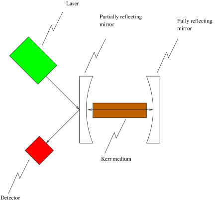
Figure 2: Schematic diagram of an optical cavity containing a Kerr medium.

A standard $(S,L,H)$ model for an optical cavity containing a Kerr medium is as follows:

$$S=I,~{}H=\left(a^{*}\right)^{2}a^{2},~{}L=\sqrt{\kappa}a;$$ (186)

e.g., see [4]. We first attempt to apply the results of Theorem 1 and Theorem 2 to this quantum system. Hence, we let

$$M=0$$

and

$$f(z,z^{*})=z^{2}\left(z^{*}\right)^{2}$$

where $z=a^{*}$. This defines a nonlinear quantum system of the form considered in Theorem 1 and Theorem 2 with $M_{1}=0$, $M_{2}=0$, $N_{1}=\sqrt{\kappa}$, $N_{2}=0$, $E_{1}=0$, $E_{2}=1$. We now investigate whether this function $f(\cdot)$ satisfies the conditions (33), (29), (30), (31), and (32). Now,

$$\frac{\partial f(z,z^{*})}{\partial z} = 2z\left(z^{*}\right)^{2};$$

$$\frac{\partial^{2}f(z,z^{*})}{\partial z^{2}} = 2\left(z^{*}\right)^{2};$$

$$\frac{\partial^{2}f(z,z^{*})}{\partial z\partial z^{*}} = 4zz^{*}.$$

Also, the sector condition (30) can be rewritten as

$$\gamma\frac{\partial f(z,z^{*})}{\partial z}^{*}\frac{\partial f(z,z^{*})}{\partial z}$$

$$\leq \frac{\partial f(z,z^{*})}{\partial z}^{*}z^{*}+z\frac{\partial f(z,z^{*})}{\partial z}+\gamma\delta_{1}$$

which is satisfied for $\gamma=0$ since

$$\frac{\partial f(z,z^{*})}{\partial z}^{*}z^{*}+z\frac{\partial f(z,z^{*})}{\partial z}=4z^{2}\left(z^{*}\right)^{2}\geq 0.$$

However this condition is not satisfied for any finite value of $\gamma>0$. Also, conditions (29), (33), (30), (31), (32) are not satisfied.

In order to overcome this difficulty, we note that any physical realization of a Kerr nonlinearity will not be exactly described by the model (186) but rather will exhibit some saturation of the Kerr effect; e.g., see [19]. In order to represent this effect, we will assume that the true function $\tilde{f}(\cdot)$ describing the Hamiltonian of the Kerr medium is such that its Taylor series expansion (3) satisfies $S_{0,k}=S_{1,k}=0$ for all $k=0,1,\ldots$ and $S_{2,2}=1$. That is, the first non-zero term in the Taylor series expansion corresponds to the standard Kerr Hamiltonian given in (186). Furthermore, we assume that the function $\tilde{f}(\cdot)$ is such that the conditions (29), (30), (31), (32), (33) are all satisfied for suitable values of the constants $\gamma>0$, $\beta>0$, $\delta_{1}\geq 0$, $\delta_{2}\geq 0$, $\delta_{3}\geq 0$. Here the quantity $\frac{1}{\gamma}$ will be proportional to the saturation limit for the Kerr nonlinearity. Thus, under these assumptions, we can assume $\tilde{f}(\cdot)\in\mathcal{W}_{1}$ and $\tilde{f}(\cdot)\in\mathcal{W}_{2}$.

This system has $F=\left[\begin{array}[]{cc}-\frac{\kappa}{2}&0\\ 0&-\frac{\kappa}{2}\end{array}\right]$, which is Hurwitz for all $\kappa>0$ and $G(s)=-\frac{2i}{s+\frac{\kappa}{2}}$. A magnitude Bode plot of this transfer function, is shown in Figure 3 for the case of $\kappa=2$.

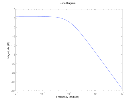
Figure 3: Magnitude Bode plot of $G(s)$ for the case $\kappa=2$.

In this case, we obtain $\|G(s)\|_{\infty}=2$ and in general

$$\|G(s)\|_{\infty}=\frac{4}{\kappa}.$$

Thus, applying Theorem 1 to this system, we can guarantee that the system is mean square stable provided

$$\kappa>\frac{4}{\gamma}.$$ (187)

We now apply our new result Theorem 2 to further analyze the stability of the system. We first choose $\kappa=2$ and construct the Popov plot corresponding to the transfer function $G(s)$ as discussed in Observation 1. For a value of $\theta=1$, this plot, along with the corresponding allowable region corresponding to $\gamma=0.1$, is shown in Figure 4. From this figure it can be seen that the Popov plot lies in the allowable region and hence, it follows from Theorem 2 and Observation 1 that this system will be mean square stable for $\kappa=2$ and $\gamma=0.1$. In fact, it follows from this plot that the frequency domain condition (50) will be satisfied for all $\gamma>0$. This condition is clearly less restrictive than the condition (187) obtained by applying Theorem 1. Furthermore, we can construct the Popov plot of the system for different values of $\kappa>0$ as shown in Figure 5. From these plots, we can see that for a suitable value of $\theta=\frac{2}{\kappa}>0$, the frequency domain condition (50) will be satisfied for all $\gamma>0$ and all $\kappa>0$. Thus, using Theorem 2, we can conclude that the optical cavity containing a saturated Kerr medium is in fact mean square stable for all $\gamma>0$ and $\kappa>0$.

\psfrag{Im}{\tiny$\omega\mathcal{I}m[G(i\omega)]$}\psfrag{Re}{\tiny$\mathcal{R}e[G(i\omega)]$}\includegraphics[width=227.62204pt]{F3.eps}

Figure 4: Popov plot for the Kerr nonlinearity system with $\kappa=2$ and $\gamma=0.1$.

\psfrag{Im}{\tiny$\omega\mathcal{I}m[G(i\omega)]$}\psfrag{Re}{\tiny$\mathcal{R}e[G(i\omega)]$}\includegraphics[width=227.62204pt]{F5.eps}

Figure 5: Popov plot for the Kerr nonlinearity system with different values of $\kappa>0$.

IV Conclusions

In this paper, we have introduced a new nonlinear quantum Popov stability criterion and applied it to the robust stability analysis of a nonlinear quantum system consisting of an optical cavity containing a Kerr medium. We have also applied an existing quantum small gain theorem to the analysis of this system. By choosing a model which represents a saturating Kerr medium, both approaches to robust stability analysis were applicable to this system. Furthermore both approaches were able to verify the robust mean square stability of this system for some range of parameter values. However, the quantum small gain theorem approach was found to be more conservative than the quantum Popov criterion approach in that it could only verify robust mean square stability for a restricted range of parameters. In contrast, the quantum Popov approach was able to verify the robust mean square stability of the system for all positive values of the system parameters.

References

[1]
R. W. Boyd, Nonlinear Optics, 3rd ed. Boston: Academic Press, 2008.
[2]
G. H. C. New, Introduction to Nonlinear Optics. Cambridge: Cambridge University Press, 2011.
[3]
H. Bachor and T. Ralph, A Guide to Experiments in Quantum Optics,
2nd ed. Weinheim, Germany: Wiley-VCH,
2004.
[4]
D. F. Walls and G. J. Milburn, Quantum Optics, 2nd ed. Berlin: Springer-Verlag, 2008.
[5]
H. M. Wiseman and G. J. Milburn, Quantum Measurement and Control. Cambridge University Press, 2010.
[6]
P. Bertet, F. R. Ong, M. Boissonneault, A. Bolduc, F. Mallet, A. C. Doherty,
A. Blais, D. Vion, and D. Esteve, “Circuit quantum electrodynamics with a
nonlinear resonator,” in Fluctuating Nonlinear Oscillators: From
Nanomechanics to Quantum Superconducting Circuits, M. Dykman, Ed. Oxford University Press, 2012.
[7]
I. R. Petersen, “Quantum robust stability of a small Josephson junction in a
resonant cavity,” in 2012 IEEE Multi-conference on Systems and
Control, Dubrovnik, Croatia, October 2012.
[8]
I. R. Petersen, V. Ugrinovskii, and M. R. James, “Robust stability of
uncertain quantum systems,” in Proceedings of the 2012 American
Control Conference, Montreal, Canada, June 2012.
[9]
J. Gough and M. R. James, “The series product and its application to quantum
feedforward and feedback networks,” IEEE Transactions on Automatic
Control, vol. 54, no. 11, pp. 2530–2544, 2009.
[10]
I. R. Petersen, V. Ugrinovskii, and M. R. James, “Robust stability of
uncertain linear quantum systems,” Philosophical Transactions of the
Royal Society A, vol. 370, no. 1979, pp. 5354–5363, 2012.
[11]
——, “Robust stability of quantum systems with a nonlinear coupling
operator,” in Proceedings of the 51st IEEE Conference on Decision and
Control, Maui, December 2012.
[12]
M. R. James, I. R. Petersen, and V. Ugrinovskii, “A Popov stability
condition for uncertain linear quantum systems,” in Proceedings of the
2013 American Control Conference, Washington, DC, June 2013, to appear,
accepted 31 Jan 2013.
[13]
H. Khalil, Nonlinear Systems, 3rd ed. Upper Saddle River, NJ, USA: Prentice-Hall, 2002.
[14]
M. R. James, H. I. Nurdin, and I. R. Petersen, “ control of linear
quantum stochastic systems,” IEEE Transactions on Automatic Control,
vol. 53, no. 8, pp. 1787–1803, 2008.
[15]
H. I. Nurdin, M. R. James, and I. R. Petersen, “Coherent quantum LQG
control,” Automatica, vol. 45, no. 8, pp. 1837–1846, 2009.
[16]
A. I. Maalouf and I. R. Petersen, “Bounded real properties for a class of
linear complex quantum systems,” IEEE Transactions on Automatic
Control, vol. 56, no. 4, pp. 786 – 801, 2011.
[17]
——, “Coherent control for a class of linear complex quantum
systems,” IEEE Transactions on Automatic Control, vol. 56, no. 2, pp.
309–319, 2011.
[18]
I. R. Petersen, “Quantum linear systems theory,” in Proceedings of the
19th International Symposium on Mathematical Theory of Networks and Systems,
Budapest, Hungary, July 2010.
[19]
B. Borchers, C. Bree, S. Birkholz, A. Demircan, and G. Steinmeyer, “Saturation
of the all-optical Kerr effect in solids,” Optics Letters, vol. 37,
no. 9, pp. 1541–1543, 2012.
[20]
M. James and J. Gough, “Quantum dissipative systems and feedback control
design by interconnection,” IEEE Transactions on Automatic Control,
vol. 55, no. 8, pp. 1806 –1821, August 2010.
[21]
J. Gough, R. Gohm, and M. Yanagisawa, “Linear quantum feedback networks,”
Physical Review A, vol. 78, p. 062104, 2008.
[22]
J. E. Gough, M. R. James, and H. I. Nurdin, “Squeezing components in linear
quantum feedback networks,” Physical Review A, vol. 81, p. 023804,
2010.