A Joint Intensity and Depth Co-Sparse Analysis Model
for Depth Map Super-Resolution

Abstract

High-resolution depth maps can be inferred from low-resolution depth measurements and an additional high-resolution intensity image of the same scene. To that end, we introduce a bimodal co-sparse analysis model, which is able to capture the interdependency of registered intensity and depth information. This model is based on the assumption that the co-supports of corresponding bimodal image structures are aligned when computed by a suitable pair of analysis operators. No analytic form of such operators exist and we propose a method for learning them from a set of registered training signals. This learning process is done offline and returns a bimodal analysis operator that is universally applicable to natural scenes. We use this to exploit the bimodal co-sparse analysis model as a prior for solving inverse problems, which leads to an efficient algorithm for depth map super-resolution.

1 Introduction

Many technical applications in fields like robotics, 3D video rendering, or human computer interaction are built upon precise knowledge of the surrounding 3D environment. This information is typically acquired either via passive or active range sensors. Passive range sensing, i.e. 3D from stereo intensity images, is essentially based on three steps. First, ambient light that is reflected from the same object surfaces is captured at multiple displaced views. Second, the disparities of corresponding light intensity samples between the different views are determined. Third, the distance to the sensor is obtained using the computed disparities together with the knowledge of the relative positions between all views. Despite very active research in this area and significant improvements over the past years, stereo methods still struggle with noise, texture-less regions, repetitive texture, and occluded areas. For an overview of stereo methods, the reader is referred to [24].

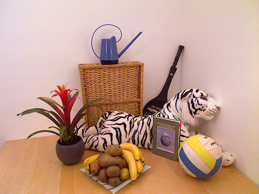
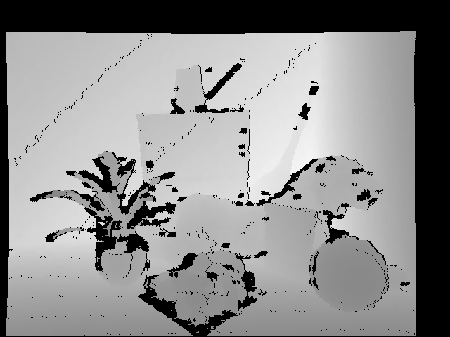
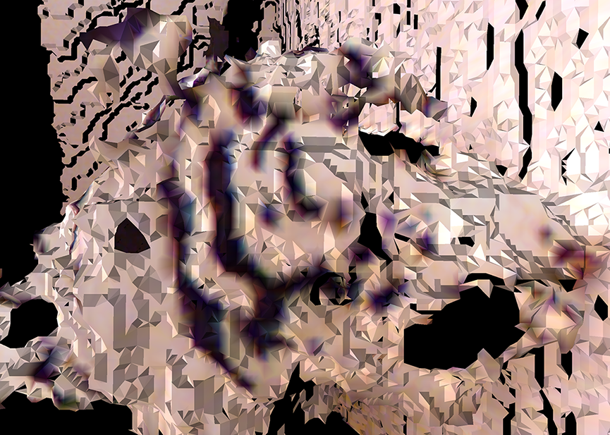
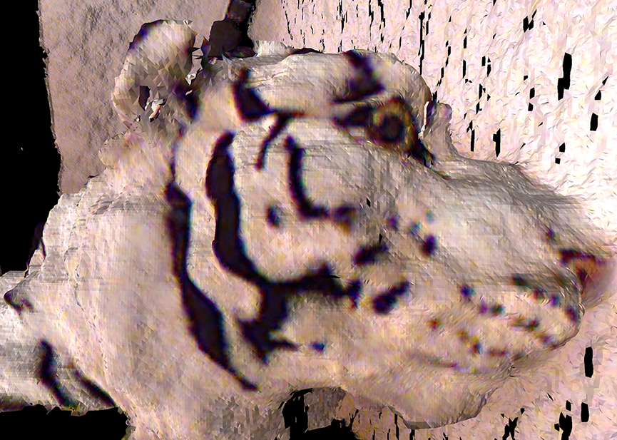
Figure 1: Top row: color image (left) and corresponding registered depth map (right) recorded by the Kinect sensor. Bottom row: a 3D rendering of the tiger head detail visualizing the difference between the original sensor data (left) and the refined version using our proposed method (right).

Active sensors, on the other hand, emit light and either measure the time-of-flight of a modulated ray, e.g. LIDAR or PMD, or capture the reflection pattern of a structured light source to infer the distance to objects, as is done for example by the well-known Microsoft Kinect. Such sensors become more and more popular, because they acquire reliable depth measurements independent of the occurring texture and are real-time capable. However, the main drawbacks are that the acquired depth maps are of low-resolution (LR) and corrupted by noisy and missing values. To overcome these limitations, different methods for upsampling and denoising LR depth maps from range sensors have been proposed, see Section 2.

A co-occurrence of signal patterns in both the depth map obtained by an active range sensor as well as in a corresponding registered camera intensity image, is suggested by the fact that both ambient and artificially emitted light is reflected by the same object surfaces. Indeed, some of the most successful methods for reconstructing and refining depth maps aim at exploiting this statistical dependency.

In this paper, we introduce a joint intensity and depth (JID) co-sparse analysis model that exploits the dependencies between the two modalities. This model is based on the assumption that the co-supports of corresponding structures are aligned when computed by a suitable pair of analysis operators. To that end, we propose a method for learning the required bimodal analysis operator from aligned training data. This procedure is done only once and offline, and results in a universally applicable operator, which is valid for all intensity and depth pairs of natural scenes. This operator together with a high-resolution (HR) intensity image is employed for reconstructing a HR depth map that corresponds to the HR intensity image. The problem is considered as a linear inverse problem, which is regularized using the bimodal analysis operator. Our numerical experiments show that our method compares favorably to state-of-the-art methods both visually and quantitatively, and they underpin the validity of our proposed joint intensity and depth data model. In summary, the two main contributions of this paper are:

• The new bimodal co-sparse analysis model that reflects the dependencies between properly aligned intensity and depth samples from the same scene.

• An algorithm for simultaneous depth map super-resolution (SR) and inpainting of missing depth values, which exploits the introduced data model and allows to cope with various noise models.

2 Related Work

Increasing the resolution of depth images obtained from range sensors has become an important research topic, and diverse approaches treating this problem have been proposed throughout the past years. Many of these methods originate from the closely related problem of intensity image super-resolution. However, these mostly aim at producing pleasantly looking results, which is different from the goal of achieving geometrically sound depth maps. Straightforward upsamling methods like nearest-neighbor, bilinear, or bicubic interpolation produce undesirable staircasing or blurring artifacts, see Figure 2. Here, we shortly review more sophisticated methods for depth map SR that aim at reducing these artifacts.

In a first attempt, methods have been proposed that use smoothing priors from edge statistics [9] or local self-similarities [10]. These methods only require a single image, but either have difficulties in textured areas, or only work well for small upscaling factors. A different approach, which also solely requires depth information is based on fusing multiple displaced LR depth maps into a single HR depth map. Schuon et al. [23] develop a global energy optimization framework employing data fidelity and geometry priors. This idea is extended for better edge-preservation by Bhavsar et al. in [4].

A number of recently introduced methods aim at exploiting co-aligned discontinuities in intensity and depth images of the same scene. They fuse the HR and LR data utilizing Markov Random Fields (MRF). Depth map refinement based on MRF has been first explored in [6], extended in [15] with a depth specific data term, and combined with depth from passive stereo in [29]. In order to better preserve local structures and to remove outliers, Park et al. [20] add a non-local means term to their MRF formulation. Aodha et al. [2] treat depth SR as an MRF labeling problem of matching LR depth map patches to HR patches from a predefined database.

Inspired by successful stereo matching algorithms, Yang et al. [28] iteratively employ a bilateral filter to improve depth SR using an additional HR intensity image. Chan et al. [5] extend this approach by incorporating a noise model specific to depth data. Xiang et al. [26] include sub-pixel accuracy, and Dolson et al. [7] address temporal coherence across a depth data stream from LIDAR scanners by combining a bilateral filter with a Gaussian framework.

Finally, methods exist that exploit the dependency between sparse representations of intensity and depth signals over appropriate dictionaries. In [11], the complex wavelet transform is used as the dictionary. Both the HR intensity image and the LR depth map are transformed into this domain and the resulting coefficients are fused using a dual tree to obtain the HR depth map. Instead of using predefined bases, approaches employing learned dictionaries are known to lead to state-of-the-art performance in diverse classical image reconstruction tasks, cf. [8, 17]. Surprisingly, applying those techniques for depth map enhancement has only very recently been explored. Mahmoudi et al. [16] first learn a depth dictionary from noisy samples, then refine and denoise these samples and finally learn an additional dictionary from the denoised samples to inpaint, denoise, and super-resolve projected depth maps from 3D models. Closest to our approach are the recent efforts of [14] and [25]. They independently learn dictionaries of depth and intensity samples, and model a coupling of the two signal types during the reconstruction phase. In [14], three dictionaries are composed from LR depth, HR depth, and HR color samples to learn a respective mapping function based on edge features. In contrast, only two dictionaries for intensity and depth are learned in [25], where the similarity of the support of corresponding sparse representations is used to model the coupling.

3 Proposed Approach

In our approach, we treat the problem of depth map super-resolution as a linear inverse problem. Basically, the goal is to reconstruct a HR depth map $\mathbf{s}\in\mathbb{R}^{n}$ from a set of measurements $\mathbf{y}\in\mathbb{R}^{m}$ that are possibly corrupted by noise and missing values, i.e. a LR depth map, with $m\leq n$. Formally, the relation between $\mathbf{s}$ and $\mathbf{y}$ is given by

$$\mathbf{y}=\mathcal{A}\mathbf{s}+\mathbf{e},$$ (1)

with $\mathcal{A}\in\mathbb{R}^{m\times n}$ modeling the sampling process, and $\mathbf{e}\in\mathbb{R}^{m}$ modeling noise and potential sampling errors. Here, the dimension $m$ of the measurement vector is significantly smaller than the dimension $n$ of the HR depth map. Consequently, reconstructing $\mathbf{s}$ in (1) is highly ill-posed. Using additional information about the signal’s structure helps to tackle this linear inverse problem.

One prior assumption that has proven useful, is that the signals of interest allow a sparse representation. A vector is called sparse, when most of its entries are equal to zero or sufficiently small in magnitude. The co-sparse analysis model [18] assumes that applying an analysis operator $\bm{\Omega}\in\mathbb{R}^{k\times n}$ with $k\geq n$ to a signal $\mathbf{s}\in\mathbb{R}^{n}$ results in a sparse vector $\bm{\Omega}\mathbf{s}\in\mathbb{R}^{k}$. If $g\colon\mathbb{R}^{k}\to\mathbb{R}$ denotes a function that measures sparsity like the $\ell_{0}$-pseudo-norm, the analysis model assumption can be exploited to tackle linear inverse problems by solving

$$\mathbf{s}^{\star}\in\arg\underset{\mathbf{s}\in\mathbb{R}^{n}}{\min}\,g(\mathbf{\Omega s})\;\text{subject to}\;d_{E}(\mathcal{A}\mathbf{s},\mathbf{y})\leq\varepsilon,$$ (2)

where $d_{E}$ denotes an appropriate error measure and $\varepsilon\in\mathbb{R}^{+}_{0}$ is an estimated upper bound of the noise energy. Typical examples for $d_{E}$ include the squared Euclidean distance.

Most crucial for the success of the analysis approach is the choice of an appropriate analysis operator. Analytic operators, e.g. the finite difference operator, exist. However, using an operator that is learned from signal examples is known to yield better performance [12, 19, 21, 27].

Our approach to depth map SR utilizes the interdependency of the two modalities intensity and depth. In a first step we describe a new data model and how it can be learned in the form of an analysis operator pair that incorporates both, signal structure and their according bimodal interdependency. In a second step, we explain how this learned prior model can be used for HR signal reconstruction.

3.1 Bimodal Co-Sparse Analysis Model

In the analysis model, the zero entries of the analyzed vector $\bm{\Omega}\mathbf{s}$ determine the signal’s structure [18]. Geometrically, $\mathbf{s}$ lies in the intersection of all hyperplanes whose normal vectors are given by the rows of $\bm{\Omega}$ indexed by the zero entries of $\bm{\Omega}\mathbf{s}$. This index set is called the co-support of $\mathbf{s}$, and is given by

$$cosupp(\bm{\Omega}\mathbf{s}):=\{j~{}|~{}(\bm{\Omega}\mathbf{s})_{j}=0\}.$$ (3)

Therein, $\mathbf{s}$ is a vectorized patch and $(\bm{\Omega}\mathbf{s})_{j}$ is the $j$-th entry of the analyzed vector. Now assume that intensity signals $\mathbf{s}_{I}\in\mathbb{R}^{n_{1}}$ as well as depth signals $\mathbf{s}_{D}\in\mathbb{R}^{n_{2}}$ allow a co-sparse representation with an appropriate pair of analysis operators $(\bm{\Omega}_{I},\bm{\Omega}_{D})\in\mathbb{R}^{k\times n_{1}}\times\mathbb{R}^{k\times n_{2}}$. Based on the knowledge that a signal’s structure is encoded in its co-support (3), we postulate that a pair of analysis operators exists such that the co-support of $\mathbf{s}_{I}$ and $\mathbf{s}_{D}$ are statistically dependent, if both signals originate from the same scene. The bimodal co-sparse analysis model assumes that the conditional probability of $j$ belonging to the co-support of $\mathbf{s}_{D}$ given that $j$ belongs to the co-support of $\mathbf{s}_{I}$ is significantly higher than the unconditional probability, i.e.

$$\begin{split}Pr(\{j\in cosupp(\bm{\Omega}_{D}\mathbf{s}_{D})\}~{}|~{}\{j\in cosupp(\bm{\Omega}_{I}\mathbf{s}_{I})\})\gg Pr(\{j\in cosupp(\bm{\Omega}_{D}\mathbf{s}_{D})\}).\end{split}$$ (4)

Clearly, this model is idealized, since in practice, the entries of the analyzed vectors are not exactly equal to zero. In the next section, we explain how the coupled pair of analysis operators $(\bm{\Omega}_{I},\bm{\Omega}_{D})$ can be jointly learned, such that aligned intensity and depth signals analyzed by these operators adhere to the introduced model.

3.2 JID Analysis Operator Learning

Generally, the goal of learning an analysis operator can be formulated as follows: Given a set ${\left\{\mathbf{s}^{(i)}\in\mathbb{R}^{n}\right\}}_{i=1}^{M}$ of training samples representing the signal class of interest, find an operator $\bm{\Omega}\in\mathbb{R}^{k\times n}$ with $k\geq n$ such that all representations $\bm{\Omega}\mathbf{s}^{(i)}$ are maximally sparse.

Here, we aim at learning the coupled pair of bimodal analysis operators $(\bm{\Omega}_{I},\bm{\Omega}_{D})\in\mathbb{R}^{k\times n_{1}}\times\mathbb{R}^{k\times n_{2}}$ for intensity and depth signals. Therefore, we use a set of $M$ aligned and corresponding training pairs $\{(\mathbf{s}_{I}^{(i)},\mathbf{s}_{D}^{(i)})\in\mathbb{R}^{n_{1}}\times\mathbb{R}^{n_{2}}\}_{i=1}^{M}$. More specifically, these are HR intensity and HR depth patches representing the same excerpt of a scene. Now, we incorporate the proposed condition (4) into the learning process by enforcing the zeros of corresponding analyzed vectors $\bm{\Omega}_{I}\mathbf{s}_{I}^{(i)},\bm{\Omega}_{D}\mathbf{s}_{D}^{(i)}$ to be at the same positions. Throughout the paper, the function $\mathbf{x}\mapsto\sum_{j=1}^{k}\log(1+\nu x_{j}^{2}),$ with $\nu>0$ being a positive weight, serves as an appropriate sparsity measure. Note, that any other smooth sparsity measure principally leads to similar results. With this, the coupled sparsity is controlled through the function

$$g(\bm{\Omega}_{I}\mathbf{s}_{I}^{(i)},\bm{\Omega}_{D}\mathbf{s}_{D}^{(i)}):=\sum\limits_{j=1}^{k}\log\bigg{(}1+\nu\big{(}(\bm{\Omega}_{I}\mathbf{s}_{I}^{(i)})_{j}^{2}+(\bm{\Omega}_{D}\mathbf{s}_{D}^{(i)})_{j}^{2}\big{)}\bigg{)}.$$ (5)

To find the ideal pair of bimodal operators we minimize the sum of squares of (5), which can be interpreted as a balanced optimization over the expectation and the variance of the analyzed vectors’ sparsity and reads as

$$G(\bm{\Omega}_{I},\bm{\Omega}_{D}):=\tfrac{1}{M}\sum\limits_{i=1}^{M}g(\bm{\Omega}_{I}\mathbf{s}_{I}^{(i)},\bm{\Omega}_{D}\mathbf{s}_{D}^{(i)})^{2}.$$ (6)

Additionally, we take separate constraints on the operator into account which are motivated in [12] and summarized in the following.

The possible solutions of the transposed of a single analysis operator are restricted to the set of full-rank matrices with normalized columns, known as the oblique manifold $\mathrm{OB}(n,k)$. Since $\mathrm{OB}(n,k)$ is open and dense in the set of matrices with normalized columns, the penalty function

$$h(\bm{\Omega}):=-\tfrac{1}{n\log(n)}\log\det(\tfrac{1}{k}\bm{\Omega}^{\top}\bm{\Omega})$$ (7)

is used to adhere to the rank condition and to prevent iterates to approach the boundary of $\mathrm{OB}(n,k)$. Furthermore, a penalty function is incorporated that enforces the operators to have distinctive rows, and which controls the mutual coherence of each operator

$$r(\bm{\Omega}):=-\sum\limits_{1\leq i<l\leq k}\log(1-({\bm{\omega}}_{i}^{\top}{\bm{\omega}}_{l})^{2}),$$ (8)

with ${\bm{\omega}}_{i}$ denoting the transposed of the $i$-th row of $\bm{\Omega}$.

Combining the two penalties into $p(\bm{\Omega}):=\kappa h(\bm{\Omega})+\mu r(\bm{\Omega}),$ with $\kappa,\mu\in\mathbb{R}^{+}$ being positive weights, and using $n_{1}=n_{2}=:n$ for legibility reasons, our problem of learning the pair of JID analysis operators is given by

$$\begin{split}\left(\bm{\Omega}_{I}^{\top},\bm{\Omega}_{D}^{\top}\right)\in\underset{\mathcal{X}_{I},\mathcal{X}_{D}\in\mathrm{OB}(n,k)}{\arg\min}&G(\mathcal{X}^{\top}_{I},\mathcal{X}^{\top}_{D})+p(\mathcal{X}^{\top}_{I})+p(\mathcal{X}^{\top}_{D}).\end{split}$$ (9)

The arising optimization problem is solved with a geometric CG method using an Armijo step size rule, cf. [1].

For the evaluation of our approach we train one fixed operator pair and use it in all presented experiments. To that end, we gather a total of $M=15000$ pairs of squared sample patches of size $\sqrt{n}=5$ from the five registered intensity and depth image pairs ’Baby1’, ’Bowling1’, ’Moebius’, ’Reindeer’ and ’Sawtooth’ of the Middlebury stereo set. As it is common in dictionary learning methods, we require all training patches to have zero-mean. Furthermore, we learn the operators with twofold redundancy, i.e. $k=2n$, resulting in the operator pair $(\bm{\Omega}_{I},\bm{\Omega}_{D})\in\mathbb{R}^{50\times 25}\times\mathbb{R}^{50\times 25}$. In general, a larger redundancy of the operators leads to better reconstruction quality but at the cost of increased computational complexity of both learning and reconstruction. Twofold redundancy provides a good trade-off between reconstruction quality and computation time. We empirically set the remaining parameters to $\nu=10$, $\kappa=9\cdot 10^{4}$ and $\mu=10^{2}$.

3.3 Depth Map Super-Resolution

In this section, we explain how the pair of patch based bimodal analysis operators $(\bm{\Omega}_{I},\bm{\Omega}_{D})$ is used to jointly reconstruct an aligned pair of intensity and depth signals $\mathbf{s}_{I},\mathbf{s}_{D}\in\mathbb{R}^{N}$ from a set of measurements $\mathbf{y}_{I}\in\mathbb{R}^{m_{1}},\mathbf{y}_{D}\in\mathbb{R}^{m_{2}}$. Here $\mathbf{s}_{I},\mathbf{s}_{D}$ are the vectorized versions of an HR intensity image and an HR depth map obtained by ordering their entries lexicographically, with $N=wh$ where $w$ and $h$ denote the height and width of both HR signals.

To use our bimodal operator for reconstructing entire images or depth maps, we need to extend the application of the operator beyond local patches. To achieve this, we recall the approach in [12] for the unimodal case. Instead of reconstructing each patch individually and combining them in a final step to form the image, the complete $N$-dimensional signal is reconstructed by minimizing the average sparsity of all patches. In this way, neighboring patches support each other during the optimization process. Accordingly, a global analysis operator $\bm{\Omega}^{F}\in\mathbb{R}^{K\times N}$ is constructed from a patch based operator $\bm{\Omega}\in\mathbb{R}^{k\times n}$. Therefore, let $\mathcal{P}_{rc}\in\mathbb{R}^{n\times N}$ denote the operator, which selects the ($\sqrt{n}\times\sqrt{n}$)-dimensional patch centered at position $(r,c)$ from the signal, then the global operator is given as

$$\bm{\Omega}^{F}:={\small\begin{bmatrix}\bm{\Omega}\mathcal{P}_{11}\\ \bm{\Omega}\mathcal{P}_{21}\\ \vdots\\ \bm{\Omega}\mathcal{P}_{hw}\end{bmatrix}}\in\mathbb{R}^{K\times N},$$ (10)

with $K=whk$, i.e. all patch positions are considered. The reflective boundary condition is used to deal with problems along boundaries.

Now, with the global operator pair $(\bm{\Omega}_{I}^{F},\bm{\Omega}_{D}^{F})$, the bimodal extension of the signal reconstruction in (2) is given by

$$\begin{split}&(\mathbf{s}^{\star}_{I},\mathbf{s}^{\star}_{D})\in\arg\underset{\mathbf{s}_{I},\mathbf{s}_{D}\in\mathbb{R}^{N}}{\min}g(\bm{\Omega}^{F}_{I}\mathbf{s}_{I},\bm{\Omega}^{F}_{D}\mathbf{s}_{D})\\ &\text{subject to}\quad d_{E}\left(\left(\mathcal{A}_{I}\mathbf{s}_{I},\mathcal{A}_{D}\mathbf{s}_{D}\right),\left(\mathbf{y}_{I},\mathbf{y}_{D}\right)\right)\leq\varepsilon.\end{split}$$ (11)

Therein, the sparsity measure $g$ is the same as the one in Equation (5). Consequently, the analyzed versions of both modalities are enforced to have a correlated co-support and hence the two signals are coupled.

The measurement matrices $\mathcal{A}_{I}\in\mathbb{R}^{m_{1}\times N}$ and $\mathcal{A}_{D}\in\mathbb{R}^{m_{2}\times N}$ model the sampling process of each modality. Here, we focus on enhancing the quality of depth measurements $\mathbf{y}_{D}$, given a fixed high quality intensity signal $\mathbf{y}_{I}=\mathbf{s}_{I}$ by simultaneously upsampling and inpainting missing measurements. In this case, $\mathcal{A}_{I}$ is the identity operator and the analyzed intensity signal is constant, i.e. $\bm{\Omega}^{F}_{I}\mathbf{s}_{I}=\mathbf{c}=\textit{const.}$ This simplifies Problem (11) for recovering a HR depth map to

$$\begin{split}&\mathbf{s}^{\star}_{D}\in\arg\underset{\mathbf{s}_{D}\in\mathbb{R}^{N}}{\min}\,g(\mathbf{c},\bm{\Omega}^{F}_{D}\mathbf{s}_{D})\\ &\text{subject to}\quad d_{E}(\mathcal{A}_{D}\mathbf{s}_{D},\mathbf{y}_{D})\leq\varepsilon_{D}.\end{split}$$ (12)

The data fidelity term $d_{E}$ depends on the error model of the depth data and can be chosen accordingly. For instance, this may be an error measure tailored to a sensor specific model, cf. Section 4.2. In this way, knowledge about the scene gained from the intensity image and its co-support regarding the bimodal analysis operators helps to determine the HR depth signal.

4 Results and Comparison

In this section we experimentally evaluate our approach by conducting two sets of experiments. First, we evaluate our approach numerically on synthetic data using the well-known Middlebury stereo dataset [22], which provides aligned intensity images and depth maps for a number of different test scenes. Second, we evaluate our method on real-world data by processing scenes captured with the popular Microsoft Kinect sensor.

4.1 Quantitative Evaluation

To compare our results to the state-of-the-art, we quantitatively evaluate our algorithm on the four standard test images ’Tsukuba’, ’Venus’, ’Teddy’, and ’Cones’ from the Middlebury dataset. To artificially create LR input depth maps, we scale the ground truth depth maps down by a factor of $d$ in both vertical and horizontal dimension. We first blur the available HR image with a Gaussian kernel of size $(2d-1)\times(2d-1)$ and standard deviation $\sigma=d/3$ before downsampling. The LR depth map and the corresponding HR intensity image are the input to our algorithm.

$d$	method	Tsukuba	Venus	Teddy	Cones
2x	nearest-neighbor	1.24	0.37	4.97	2.51
	Yang et al. [28]	1.16	0.25	2.43	2.39
	Hawe et al. [12]	1.03	0.22	2.95	3.56
	our method	0.47	0.09	1.41	1.81
4x	nearest-neighbor	3.53	0.81	6.71	5.44
	Yang et al.	2.56	0.42	5.95	4.76
	Hawe et al.	2.95	0.65	4.80	6.54
	our method	1.73	0.25	3.54	5.16
8x	nearest-neighbor	3.56	1.90	10.9	10.4
	Yang et al.	6.95	1.19	11.50	11.00
	Lu et al. [15]	5.09	1.00	9.87	11.30
	Hawe et al.	5.59	1.24	11.40	12.30
	our method	3.53	0.33	6.49	9.22

Table 1: Numerical comparison of our method to other depth map SR approaches for different upscaling factors $d$. The figures represent the percentage of bad pixels with respect to all pixels of the ground truth data and an error threshold of $\delta=1$.

$d$	method	Tsukuba	Venus	Teddy	Cones
2x	nearest-neighbor	0.612	0.288	1.543	1.531
	Chan et al. [5]	n/a	0.216	1.023	1.353
	Aodha et al. [2]	0.601	0.296	0.977	1.227
	Hawe et al. [12]	0.278	0.105	0.996	0.939
	our method	0.255	0.075	0.702	0.680
4x	nearest-neighbor	1.189	0.408	1.943	2.470
	Chan et al.	n/a	0.273	1.125	1.450
	Aodha et al.	0.833	0.395	1.184	1.779
	Hawe et al.	0.450	0.179	1.389	1.398
	our method	0.487	0.129	1.347	1.383
8x	nearest-neighbor	1.135	0.546	2.614	3.260
	Chan et al.	n/a	0.369	1.410	1.635
	Hawe et al.	0.713	0.249	1.743	1.883
	our method	0.753	0.156	1.662	1.871

Table 2: Numerical comparison of our method to other depth map SR approaches. The figures represent the RMSE in comparison with the ground truth depth map.

Here, we assume an i.i.d. normal distribution of the error, which leads to the data fidelity term $d_{E}(\mathcal{A}_{D}\mathbf{s}_{D},\mathbf{y}_{D})=\|\mathcal{A}_{D}\mathbf{s}_{D}-\mathbf{y}_{D}\|^{2}_{2}$. From (12) we get the unconstrained optimization problem for reconstructing the HR depth signal as

$$\mathbf{s}^{\star}_{D}\in\underset{\mathbf{s}_{D}\in\mathbb{R}^{N}}{\arg\min}\,\lambda g(\mathbf{c},\bm{\Omega}^{F}_{D}\mathbf{s}_{D})+\|\mathcal{A}_{D}\mathbf{s}_{D}-\mathbf{y}_{D}\|^{2}_{2}.$$ (13)

Larger values of the weighting factor $\lambda\propto\varepsilon^{-1}_{D}$ lead to a faster convergence of the algorithm but may cause larger differences between the measurements and the reconstructed depth map. To achieve the best results with few iterations, we start with $\lambda=1$ and restart the conjugate gradient optimization procedure five times, while consecutively shrinking the multiplier to a final value of $\lambda=10^{-2}$.

Following the methodology described in the work of comparable depth map SR approaches, we use the Middlebury stereo matching online evaluation tool to quantitatively assess the accuracy of our results with respect to the ground truth data. We report the percentage of bad pixels over all pixels in the depth map with an error threshold of $\delta=1$. Additionally, we provide the root-mean-square error (RMSE) based on 8-bit images. We rely on the results reported by the authors of comparable methods regarding the numerical comparison in Table 1 and Table 2, since an implementation is not publicly available. To show the advantage of enforcing a coupled co-support in the analysis formulation, we further employed a single modal operator learned by the code provided by the authors of [12]. This operator has been learned from the same training images as described above, and with the parameters documented in their paper.

As illustrated in Figure 2, our method improves depth map SR considerably over simple interpolation approaches. Neither staircasing nor substantial blurring artifacts occur, particularly in areas with discontinuities. Also, there is no noticeable texture cross-talk in areas of smooth depth and cluttered intensity. Edges can be preserved with great detail due to the additional knowledge provided by the intensity image, even if SR is conducted using large upscaling factors. The quantitative comparison with other depth map SR methods demonstrates the superior performance of our JID analysis operator across all test images. It reaches near perfect results for small upscaling factors and the improvement over state-of-the-art methods is of particular significance for larger magnification factors. We refer the reader to the supplementary material for illustrations of our synthetic test results.

(a) ground truth

(b) nearest neighbor

(c) bicubic

(d) proposed method

Figure 2: Visual comparison of different upscaling methods on a detail in the test image Tsukuba from [22] which was downsampled by a factor of 8 in both vertical and horizontal direction.

4.2 Validation on Kinect Data

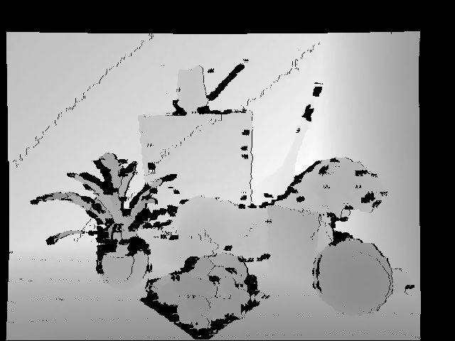
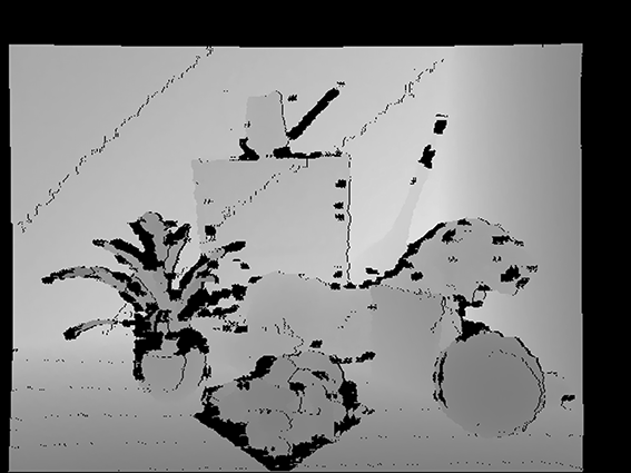
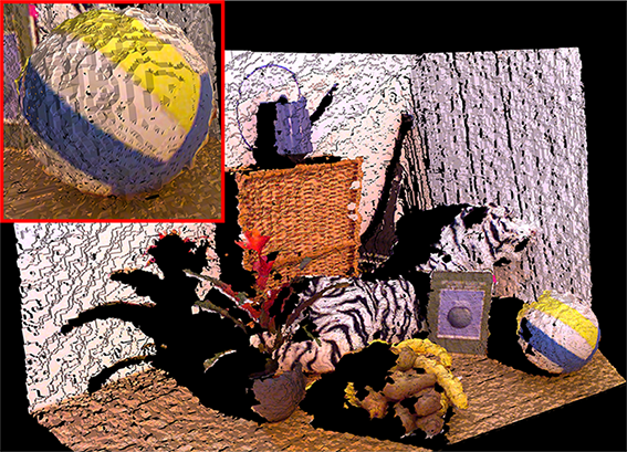
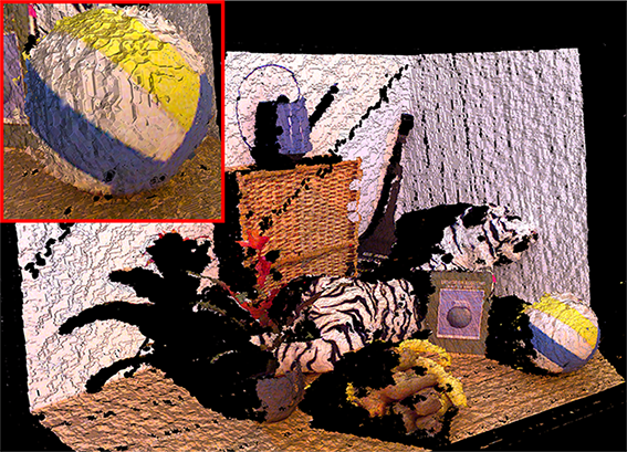
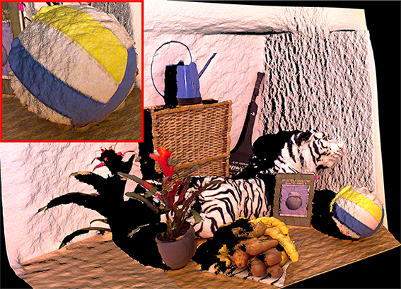
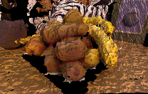
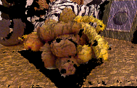
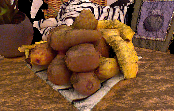
Figure 3: Depth maps (top row), 3D rendering of Kinect color and depth data depicting the entire scene (middle row) and a detail of the fruit bowl (bottom row). Left column: original Kinect data like in the top row of Figure 1 with downsampled color information, center column: bicubic interpolation (1280x960), right column: proposed method (1280x960). Note that object shadows are due to the single view occlusion.

In order to demonstrate the applicability of our algorithm to real data, we captured color images of size 1280x960 and corresponding depth maps of size 640x480 using the Microsoft Kinect sensor and then upscale the depth map by a factor of $d=2$ to match its size to the one of the color image.

Since the approximate error statistics for this application and this sensor have been studied previously in [13], we can use this information to further refine our data model. According to [13], the standard deviation of Kinect depth data is proportional to the square of the depth value $\sigma_{i}\propto(y_{D}^{(i)})^{2}$. We utilize this in our error model by employing the squared Mahalanobis distance for $d_{E}$ in (12), which yields

$$\mathbf{s}^{\star}_{D}\in\underset{\mathbf{s}_{D}\in\mathbb{R}^{N}}{\arg\min}\,\lambda g(\mathbf{c},\bm{\Omega}^{F}_{D}\mathbf{s}_{D})+d_{E}\left(\mathcal{A}_{D}\mathbf{s}_{D},\mathbf{y}_{D}\right),$$ (14)

where $d_{E}=\left(\mathcal{A}_{D}\mathbf{s}_{D}-\mathbf{y}_{D}\right)^{\top}\bm{\Sigma}^{-1}\left(\mathcal{A}_{D}\mathbf{s}_{D}-\mathbf{y}_{D}\right)$ and $\bm{\Sigma}\in\mathbb{R}^{m_{2}\times m_{2}}$ being a diagonal matrix with main diagonal elements $(y_{D}^{(i)})^{2}$.

As the Kinect sensor uses structured light to measure depth, the signal is corrupted by missing pixels due to occlusions arising from the displacement of the IR light source and the sensor. To fill these gaps in the data, we model the measurement matrix in such a way that it excludes these gaps from the sampling process of the LR depth image, i.e. removing the rows of $\mathcal{A}$ that correspond to zero entries in $\mathbf{y}_{D}$. As a result, we perform inpainting of missing depth values without any additional processing, while simultaneously increasing the depth map resolution. By this, we handle two of the main issues of Kinect data in one step.

To our knowledge, there is no data set publicly available that allows to numerically evaluate Kinect depth map enhancing methods by providing ground truth data. Therefore, we assess the quality of the super-resolved Kinect depth maps visually. Since small differences in the depth map represented as a gray-scale image are almost invisible to the naked eye, we illustrate our results in Figure 3 using ball pivoting surface reconstruction [3] on a point cloud that we created from the depth map computed by our algorithm. As it can be seen, our method does not only increase the details in the 3D scene significantly, but also treats the missing pixels with great success. This is especially obvious in the details of the tiger head in Figure 1 and the fruit bowl in Figure 3. The 3D rendering illustrates the impact of the bimodal support during reconstruction particularly around depth discontinuities, but it also leads to smoother surfaces of table and wall due to the smooth texture of the corresponding intensity signal.

We would like to emphasize that we use the same JID analysis operators as in the Middlebury experiments in Section 4.1, even though the training data was captured using a different sensor technology than the Kinect. This underpins that the prior model we learn is general enough to be used for high quality reconstruction of both synthetic and real world data.

5 Conclusion and Discussion

Figure 4: Plot of the relative RMSE over the optimization iterations for the upscaling of the synthetic test images by a factor of $8$.

We proposed an approach for inferring high-resolution depth maps from low-resolution depth samples given an additional high-resolution intensity image of the scene. We present an extension of the co-sparse analysis model to the bimodal case. The required pair of analysis operators is learned jointly such that the co-sparse representation of a pair of corresponding intensity and depth samples have a correlated co-support. This data model is employed for depth map super resolution and yields improved results on the benchmark data set over state-of-the-art methods. Moreover, it greatly improves real-world depth data recorded by a Kinect sensor. The fact that the same pre-trained operators can be used to refine both synthetic as well as real-world depth maps, underpins the validity of the model assumptions and emphasizes the capability of this method to abstract training data appropriately.

Despite these compelling results, our method certainly has a few limitations. We showed that missing pixels can be recovered very successfully with our approach. However, the local assumptions fail if the missing areas in the input signal are too large. As a results, inpainting of such large gaps may be inaccurate if the global support in our reconstruction model is insufficient to overcome this. For instance, this can be observed in the frame of missing pixels around the depth map in Figure 3, which is due to registering intensity and depth inputs. Finally, in our current implementation, reconstructing a HR depth image with $500$ iterations takes up to three minutes on a single 3.2 GHz CPU with unoptimized Matlab code. Since most of the processing time is dedicated to parallelizable filtering operations, we expect to improve on this with a better software implementation and processing on a GPU. Furthermore, the number of iteration in the reconstruction may be reduced significantly. As shown in Figure 4, the last $400$ iterations only reduce the RMSE by about $0.2$% and very descent recovery results are achieved with only $50$ optimization steps.

References

- [1] P. A. Absil, R. Mahony, and R. Sepulchre. Optimization Algorithms on Matrix Manifolds. Princeton University Press, 2008.
- [2] O. M. Aodha, N. D. F. Campbell, A. Nair, and G. J. Brostow. Patch Based Synthesis for Single Depth Image Super-Resolution. In ECCV, 2012.
- [3] F. Bernardini, J. Mittleman, H. Rushmeier, C. Silva, and G. Taubin. The ball-pivoting algorithm for surface reconstruction. IEEE Transactions on Visualization and Computer Graphics, 5(4):349–359, 1999.
- [4] A. V. Bhavsar and A. N. Rajagopalan. Range Map Superresolution-Inpainting, and Reconstruction from Sparse Data. Computer Vision and Image Understanding, 116(4):572–591, 2012.
- [5] D. Chan, H. Buisman, C. Theobalt, and S. Thrun. A Noise-Aware Filter for Real-Time Depth Upsampling. In Workshop on Multi-camera and Multi-modal Sensor Fusion Algorithms and Applications, 2008.
- [6] J. Diebel and S. Thrun. An Application of Markov Random Fields to Range Sensing. In NIPS, volume 18, pages 291–298, 2005.
- [7] J. Dolson, J. Baek, C. Plagemann, and S. Thrun. Upsampling Range Data in Dynamic Environments. In CVPR, pages 1141–1148, 2010.
- [8] M. Elad, M. A. T. Figueiredo, and Y. Ma. On the Role of Sparse and Redundant Representations in Image Processing. IEEE Proceedings, 98(6):972–982, 2010.
- [9] R. Fattal. Image Upsampling via Imposed Edge Statistics. ACM Transactions on Graphics, 26(3), 2007.
- [10] G. Freedman and R. Fattal. Image and Video Upscaling from Local Self-Examples. ACM Transactions on Graphics, 30(2):1–11, 2011.
- [11] S. A. Gudmundsson and J. R. Sveinsson. ToF-CCD Image Fusion using Complex Wavelets. In ICASSP, pages 1557–1560, 2011.
- [12] S. Hawe, M. Kleinsteuber, and K. Diepold. Analysis Operator Learning and Its Application to Image Reconstruction. IEEE Transactions on Image Processing, 22(6):2138–2150, 2013.
- [13] K. Khoshelham and S. O. Elberink. Accuracy and resolution of Kinect depth data for indoor mapping applications. Sensors, 12(2):1437–1454, 2012.
- [14] Y. Li, T. Xue, L. Sun, and J. Liu. Joint Example-Based Depth Map Super-Resolution. In IEEE International Conference on Multimedia and Expo, pages 152–157, 2012.
- [15] J. Lu, D. Min, R. S. Pahwa, and M. N. Do. A Revisit to MRF-Based Depth Map Super-Resolution and Enhancement. In ICASSP, pages 985–988, 2011.
- [16] M. Mahmoudi and G. Sapiro. Sparse Representations for Range Data Restoration. IEEE Transactions on Image Processing, 21(5):2909–2915, 2012.
- [17] J. Mairal, M. Elad, and G. Sapiro. Sparse Representation for Color Image Restoration. IEEE Transactions on Image Processing, 17(1):53–69, 2008.
- [18] S. Nam, M. E. Davies, M. Elad, and R. Gribonval. The Cosparse Analysis Model and Algorithms. Applied and Computational Harmonic Analysis, 34(1):30–56, 2013.
- [19] B. Ophir, M. Elad, N. Bertin, and M. D. Plumbley. Sequential Minimal Eigenvalues - An Approach to Analysis Dictionary Learning. In EUSIPCO, pages 1465–1469, 2011.
- [20] J. Park, H. Kim, M. S. Brown, and I. Kweon. High Quality Depth Map Upsampling for 3D-TOF Cameras. In ICCV, pages 1623–1630, 2011.
- [21] R. Rubinstein, T. Peleg, and M. Elad. Analysis K-SVD: A Dictionary-Learning Algorithm for the Analysis Sparse Model. IEEE Transactions on Signal Processing, Available online, 2012.
- [22] D. Scharstein and R. Szeliski. High-Accuracy Stereo Depth Maps using Structured Light. In CVPR, pages 195–202, 2003.
- [23] S. Schuon, C. Theobalt, J. Davis, and S. Thrun. LidarBoost: Depth Superresolution for ToF 3D Shape Scanning. In CVPR, pages 343–350, 2009.
- [24] S. M. Seitz, B. Curless, J. Diebel, D. Scharstein, and R. Szeliski. A Comparison and Evaluation of Multi-View Stereo Reconstruction Algorithms. In CVPR, volume 1, pages 519–528, 2006.
- [25] I. Tosic and S. Drewes. Learning Joint Intensity-Depth Sparse Representations. arXiv preprint, 2012. arXiv:1201.0566v1.
- [26] X. Xiang, G. Li, J. Tong, and Z. Pan. Fast and Simple Super Resolution for Range Data. In International Conference on Cyberworlds, pages 319–324, 2010.
- [27] M. Yaghoobi, S. Nam, R. Gribonval, and M. E. Davies. Analysis Operator Learning for Overcomplete Cosparse Representations. In EUSIPCO, pages 1470–1474, 2011.
- [28] Q. Yang, R. Yang, J. Davis, and D. Nistér. Spatial-Depth Super Resolution for Range Images. In CVPR, pages 1–8, 2007.
- [29] J. Zhu, L. Wang, R. Yang, and J. Davis. Fusion of Time-of-Flight Depth and Stereo for High Accuracy Depth Maps. In CVPR, pages 1–8, 2008.