Explicit force formlulas for two dimensional potential flow with multiple bodies and multiple free vortices

Abstract

For problems with multiple bodies, the current integral approach needs the use of auxiliary potential functions in order to have an individual force formula for each body. While the singularity approach, based on an extension of the unsteady Lagally theorem, is restricted to multibody and multivortex flows without bound vortex and vortex production. In this paper, we consider multibody and multivortex flow and derive force formulas, in both forms of singularity approach and integral approach but without auxiliary function, that give individual forces of each body for unsteady two dimensional potential flow with vortex production on the surface of bodies. A number of problems, including Karman vortex street, Wagner problem of impulsively starting flow, interaction of two circular cylinders with circulation, and interaction of an airfoil with a bound vortex, are used to validate the force formulas.

Keywords. lift force, drag force, multibody, multiple vortices

1 Introduction

In the classic Kutta Joukowski theorem, the role of the starting vortex, produced during the starting up of flow, is omitted by simply assuming it disappear in the far flow field. Thus the lift is related to the circulation of bound vortex (Batchelor 1967). Under the assumption of steady potential flow, the circulation of the bound vortex is determined by the Kutta condition, due to which the role of viscosity is implicitly incorporated though explicitly ignored (Grighton 1985). The lift predicted by Kutta Joukowski theorem within the framework of inviscid flow theory is quite accurate even for real viscous flow, provided the flow is steady and unseparated, see Anderson (1984,p.192) for more details.

For many problems, there may be free vortices, including the starting vortex, or other bodies close to the body. These problems have been attracting great attentions since more than two decades ago, due to their wide applications in unsteady flows (Chow&Huang 1982, Lee&Smith 1991, Aref 2007) and in multibody flows such as multi-turbine flow (Oterberg, 2010), multi-blade flow (Smith & Timoshin, 1996),  multi-element airfoil flow (Katz & Plotkin, 2001), multi-wing aerodynamics as for dragonfly (Hsieh, Kung&Chang 2010), and flows in staggered cylinders (Crowdy 2006).  Early studies considering the interaction of a vortex with a wing can be found in Saffman (1992,p122). The recent studies led to force formulas which can be conveniently classified into integral approaches and singularity approaches. For integral approaches, the forces are expressed in terms of the time variation of the integrated vorticity moment or fluid impulse. For singularity approaches, the forces are expressed in terms of the production of the strengths of singularities and the speeds of the real and image singularities. In both approaches, there may be additional terms, including for instance the added mass effect, if the body is subjected to acceleration, rotation and deformation.

The major differences between various integral approaches lie on the choice of the integration domain. The integral approaches of Wu (1981) for viscous flow and Saffman (1992) for inviscid flow use integrals defined for the whole space including both the fluid region and the solid region. With the help of auxiliary flow potentials, Howe (1995) derived an integral approach with a surface integral for the viscous force but with the volume integral only defined for the space occupied by the fluid and with the contribution from added mass, pressure by vortices and skin frictions represented by separate terms. Such an approach has been subsequently extended to multiple bodies by Ragazzo & Tabak (2007) and Chang, Yang & Chu (2008).  The advantage of the integral approach is that it only requires the knowledge of the velocity field and its derivatives. The disadvantage is that the vortices in the far flow field, such as starting vortices, must also be taken into account, even when the starting vortices are at infinity. Integral approaches for a truncated domain are then derived, at the sacrifice of introducing boundary surface integrals (Noca et al 1999, Wu et al 2007, Eames et al 2008), see Wu, Lu& Zhuang (2007) for more recent advances related to integral approaches and for a thorough discussion of the usefulness of the various integral approaches.

The force formulas by the singularity approach are basically worked out through using the complex potential theory and the unsteady Blasius theorem. The Blasius equation for the general case of unsteady flow and for a body in arbitrary motion can be found in Thomson (1968). Streitlien and Triantafyllou (1995) derived a force formula for a single Joukowski airfoil surrounded with point vortices convected freely. Ramodanov (2002) considered the motion of a circular cylinder in the presence of N point vortices and the forces are expressed in terms of the speeds of both real and image vortices. Kanso&Oskouei (2008) extended these formulas to deformable bodies with vortex production. The forces are also expressed in terms of the velocities of real vortices plus the time variation of an additional integral term representing all the effects other than the motion of vortices outside of the cylinder, see Shashikanth et al (2002) for a circular cylinder, Borisov et al (2007)  for a general cylinder, and Michelin& Smith (2010) for problems with vortex production.

For singularity approaches, both the real and image vortices are implicitly or explicitly included locally according to their real positions. For the case of an airfoil interacting with one outside vortex, Katz and Plotkin (2001, chapter 6.9) express the force in terms of the induced velocity at the body center. The role of real vortex outside of the body is represented by the induced velocity at the body center. This result was obtained under the lumped vortex assumption and extended to the case of multi-airfoil and multi-vortex flow by Bai&Wu (2013). The presence of singularities such as sources and doublets outside of a body has been also studied in the framework of Lagally theorem (Milne-Thomson 1968, Landweber&Miloh1980). Wu, Yang &Young (2012) extended the Lagally theorem to the case of two dimensional flow with multibody moving in a still fluid in the presence of multiple free vortices, and the forces are expressed in terms of the induced velocities or its derivatives at the positions of the internal singularities, including sources, doublets and image vortices. Bound vortex and vortex production are not considered in this work. Moreover, validation and application studies are restricted to circular cylinders.

For convenience, the approaches purely based on the velocities of singularities will be called singularity velocity method. When the induced flow velocities at the inner singularities are used to replace the velocities of the free singularities, the approach will be called induced velocity method.

In this paper, we consider unsteady two dimensional potential flow with multiple bodies and multiple free vortices. Each body is assumed to have an arbitrary shape and vortex production is also considered. Force formulas, algebraic and explicit for each body, valid for both discrete and continuously distributed singularities, will be derived. This paper will be organized as follows.

In section 2  we first use a momentum approach to relate the lift force and induced drag force to the speeds of singularities inside and outside of a single body (singularity velocity method) with and without vortex production. We then relate the force terms due to the outside singularities to the induced velocities inside the body and express the forces in terms of the relative induced velocities and strengths of singularities inside of the body (induced velocity method). The induced velocity method is then extended to the case of multibody flow. Both the singularity velocity method and the induced velocity method, for discrete singularities, are finally extended to the case of continuously distributed vortices, sources and doublets.

In section 3, we use three problems to show how to use or to validate the force formulas. The first problem is for circular cylinders for which the method of images can be used to obtain the singularities. Notably, we will consider the interaction of two circular cylinders with given bound vortices, for which Crowdy (2006) gives exact solution. The second problem is the drag for Karman vortex street, a very difficulty problem since the drag is not related to the shape of the body.  The last problem is the interaction of a free vortex with an airfoil, including the well known example of impulsively starting flow with vortex shedding. Finally we will consider an application, a bound vortex above the middle point of a flat plate.

A short summary, with emphasis on the new features of the present work and remaining work to be done, is provided in section 4.

2 Force formulas in various forms

In this section, we first state the flow field to be considered. Then we use a momentum approach based on a suitably designed control volume to obtain a force formula. Then this force formula is rewritten in a form such that the forces are only related to flow properties inside the body. Finally the force formulas will be extended to multibody flow and to flows with continuous distribution of vortices, sources and doublets. Important remarks, including relation and difference to other theories and the treatment of vortex production forces, will also be provided.

2.1 Description of the flow field

Consider a body with infinite span, immersed in an incompressible two-dimensional flow at constant density $\rho$. The freestream velocity $V_{\infty}$ is assumed horizontal. The local flow field is supposed to be generated by vortices, sources, doublets and body acceleration and rotation, in a way that the total velocity of the flow can be obtained by a linear superposition of the induced velocities due to these factors. Singularities, including point vortices, sources and doublets, are assumed to be either inside of the body (called inner ones) or outside of the body (called outer ones). Each of the outer singularities will be assumed to be at a finite distance to the body.

The sum of the strengths of the inner vortices is equal to $\Gamma_{b}=\int_{\partial A}\left(udx+vdy\right)$, which is just the circulation of the bound vortex, the closed curve $\partial A$ is along the body with an anticlockwise path, so that a clockwise circulation has a negative sign. We note that even when there is vortex production, the conservation of total circulation holds

$$\underset{i}{\sum}\frac{d\Gamma_{i}}{dt}=0.$$ (1)

A singularity, located at $(x_{i},y_{i})$ but generally moving at the velocity $\left(\frac{dx_{i}}{dt},\frac{dy_{i}}{dt}\right)$, will be either a point vortex of strength $\Gamma_{i}$, a source of strength $m_{i}$, or a doublet of strength $\mu_{i}$.

The (fluid) velocity induced at $(x,y)$ by a point vortex $(i)$ at $(x_{i},y_{i})$ is

$$\left\{\begin{array}[]{c}u^{(i)}(x,y)=\frac{\partial\psi_{i}}{\partial y}=\frac{\partial\phi_{i}}{\partial x}=-\frac{\Gamma_{i}}{2\pi}\frac{y-y_{i}}{r_{i}^{2}}\\ v^{(i)}(x,y)=-\frac{\partial\psi_{i}}{\partial x}=\frac{\partial\phi_{i}}{\partial y}=\frac{\Gamma_{i}}{2\pi}\frac{x-x_{i}}{r_{i}^{2}}\end{array}\right.$$ (2)

where $\psi_{i}=-\frac{\Gamma_{i}}{2\pi}\ln r_{i}$ with $r_{i}=\sqrt{(x-x_{i})^{2}+(y-y_{i})^{2}}$ is the stream function and $\phi_{i}=\frac{\Gamma_{i}\theta_{i}}{2\pi}$ is the velocity potential. The angle $\theta_{i}$ is defined such that $x-x_{i}=r_{i}\cos\theta_{i}$ and $y-y_{i}=r_{i}\sin\theta_{i}$.  It should be emphasized that this induced velocity is independent of the velocity of the vortex.

A doublet can be treated equivalently as a vortex pair (Thomson 1968,p361), see at the end of section 2.3. Thus we first assume the doublets have been transformed into vortices and just derive forces due to vortices and sources, then the explicit influence due to doublets will be derived directly from the vortex based forces (section 2.3).

Pure source (sink) singularities are in fact not required since we only consider closed bodies, for which we may always use a number of source doublets to represent pure sources. But for completeness we will also consider the existence of sources. The flow field due to a point source $(i)$ of strength $m_{i}$ is

$$\left\{\begin{array}[]{c}u^{(i)}(x,y)=\frac{\partial\psi_{i}}{\partial y}=\frac{\partial\phi_{i}}{\partial x}=\frac{m_{i}}{2\pi}\frac{x-x_{i}}{r_{i}^{2}}\\ v^{(i)}(x,y)=-\frac{\partial\psi_{i}}{\partial x}=\frac{\partial\phi_{i}}{\partial y}=\frac{m_{i}}{2\pi}\frac{y-y_{i}}{r_{i}^{2}}\end{array}\right.$$ (3)

Since the functional forms for (3) and (2) are similar, the forces due to sources can be similarly obtained as for vortices.

Now consider body generated flow, for a body ($A$) rotating at the angular speed $\Omega$ (positive if anticlockwise) around the point ($x_{o},y_{o}$) which translates in addition at velocity $(U,V)$ in a flow already with a free stream velocity $V_{\infty}$.  The flow potential and stream function due to body translation and rotation may be decomposed as

$$\phi_{b}=U\phi_{U}+V\phi_{V}+\Omega\phi_{\Omega}\text{, \ }\psi_{b}=U\psi_{U}+V\psi_{V}+\Omega\psi_{\Omega}\text{\ }$$ (4)

where $\phi_{U},\phi_{V},\phi_{\Omega}$ and $\psi_{U},\psi_{V},\psi_{\Omega}$ are the so called normalized  potentials and stream functions, generated by the body translating and rotating at unitary speed. The forces due to this will be related to added mass effects.

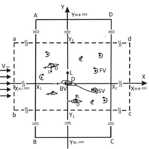
Figure 1: Ccontrol volumes: the solid box ABCD defines a vertical control volume $(X_{1},X_{2})\times(-\infty,\infty)$  and the dashed box abcd defines a horizontal control volume $(-\infty,\infty)\times(Y_{1},Y_{2})$.

2.2 Singularity velocity method

Now we use a momentum balance approach, based on the control volumes (vertical control volume and horizontal control volume) defined in Fig.1, to study the forces. The use of two types of control volumes is just for simplification of some algebraic operations during the derivation of forces.

We assume the boundaries of the control volume to be far enough away from the body and singularities, so that the momentum balance approach used here will be linear and therefore the contributions by various singularities (when the body is regarded fixed) and by body generated flow (when the body is accelerating and rotating) can be decomposed.

A) forces due to vortices. For lift, we use the vertical control volume for momentum balance. The body is subjected to a lift force $(L_{v})$, due to vortices, so that the fluid in the control volume is subjected to a force of equal magnitude but with an opposite direction, and this force is balanced by the momentum flux across the left and right boundaries $(x=X_{1}$, $x=X_{2}$) and the time variation of the momentum inside the control volume excluding the body, i.e.,

$${\normalsize L}_{v}{\normalsize=\rho\underset{i}{\sum}\int_{x=x_{1}}V_{\infty}v^{(i)}dy-\rho\underset{i}{\sum}\int_{x=x_{2}}V_{\infty}v^{(i)}dy-}\underset{i}{\sum}\frac{dm_{y}^{(i)}}{dt}+L_{av}$$ (5)

The last two terms on the right hand side represent the momentum change in the control volume excluding the region occupied by the body. Hence if $\frac{dm_{y}^{(i)}}{dt}$ is defined for the whole space in the control volume, i.e.,

$$\frac{dm_{y}^{(i)}}{dt}=\frac{d}{dt}\overset{X_{2}}{\underset{X_{1}}{\int}}\overset{\infty}{\underset{-\infty}{\int}}\rho v^{(i)}dydx$$

then, $L_{av}$ represents the momentum variation rate of the fictitious fluid inside the body. The specific role of $L_{av}$ will be further discussed in the end of this subsection.

To find the explicit form of the integrals involved in (5), we use the identity

$$\int_{-\infty}^{\infty}\frac{c}{b^{2}+(y-d)^{2}}dy=\frac{\pi c}{\left|b\right|}$$

which holds for any set of parameters $b,c,d$ independent of $y$. Hence

$$\left\{\begin{array}[]{l}\rho\overset{\infty}{\underset{-\infty}{\int}}\left.V_{\infty}v^{(i)}\right|_{X_{1}}dy=\frac{\rho V_{\infty}\Gamma_{i}}{2}\frac{X_{1}-x_{i}}{\left|X_{1}-x_{i}\right|}=-\frac{1}{2}\rho V_{\infty}\Gamma_{i}\\ \rho\overset{\infty}{\underset{-\infty}{\int}}\left.V_{\infty}v^{(i)}\right|_{X_{2}}dy=\frac{\rho V_{\infty}\Gamma_{i}}{2}\frac{X_{2}-x_{i}}{\left|X_{2}-x_{i}\right|}=\frac{1}{2}\rho V_{\infty}\Gamma_{i}\\ \frac{d}{dt}\overset{X_{2}}{\underset{X_{1}}{\int}}\overset{\infty}{\underset{-\infty}{\int}}\rho v^{(i)}dydx=\rho\frac{1}{2\pi}\frac{d}{dt}\left(\Gamma_{i}\overset{x_{i}}{\underset{X_{1}}{\int}}\frac{\pi(x-x_{i})}{\left|x-x_{i}\right|}+\Gamma_{i}\overset{X_{2}}{\underset{x_{i}}{\int}}\frac{\pi(x-x_{i})}{\left|x-x_{i}\right|}\right)dx\\ \text{ \ \ \ \ \ \ \ \ \ \ \ \ \ \ \ }=\rho\frac{1}{2\pi}\frac{d}{dt}\left(-\pi\left(x_{i}-X_{1}\right)\Gamma_{i}+\pi\left(X_{2}-x_{i}\right)\Gamma_{i}\right)\\ \text{ \ \ \ \ \ \ \ \ \ \ \ \ \ \ \ }=-\rho\Gamma_{i}\frac{d\left(\Gamma_{i}x_{i}\right)}{dt}+\rho\frac{1}{2\pi}\left(\pi(X_{2}+X_{1})\right)\frac{d\Gamma_{i}}{dt}\end{array}\right.$$

Inserting these formulas into (5) we get

$$L_{v}=-\rho\underset{i}{\sum}\left(V_{\infty}\Gamma_{i}-\frac{d\left(\Gamma_{i}x_{i}\right)}{dt}\right)+L_{av}+\rho\frac{1}{2\pi}\left(\pi(X_{2}+X_{1})\right)\underset{i}{\sum}\frac{d\Gamma_{i}}{dt}$$

Using (1) to eliminate the last term on the right hand side we obtain

$$L_{v}=-\rho\underset{i}{\sum}\left(V_{\infty}\Gamma_{i}-\frac{d\left(\Gamma_{i}x_{i}\right)}{dt}\right)+L_{av}$$ (6)

Similarly, by using the horizontal control volume, we obtain the drag force formula

$$D_{v}=-\rho\underset{i}{\sum}\frac{d\left(\Gamma_{i}y_{i}\right)}{dt}+D_{av}$$ (7)

where $D_{av}$ represents the change of $x$-momentum inside the body.

B) forces due to sources.  As remarked in the last subsection, the functional form of the velocity components $u$ and $v$ due to a point source is the same as that of $v$ and $-u$ for a vortex. Hence we can use the results of vortices and directly write down the force formulas for point sources as

$$L_{st}=\rho\underset{i}{\sum}\frac{d\left(m_{i}y_{i}\right)}{dt}+L_{as},D_{st}=\rho\underset{i}{\sum}\frac{d\left(m_{i}x_{i}\right)}{dt}+D_{as}$$ (8)

and $L_{as}$ and $D_{as}$ represent the momentum change inside the body due to sources.

C) momentum change inside the body. Now consider the momentum changes inside the body due to vortices ($L_{av},D_{av}$) and sources ($L_{as},D_{as}$). With  $L_{a}=L_{av}+L_{as}$ and $D_{a}=D_{av}+D_{as}$ we may write

$$L_{a}=\underset{i}{\sum}\frac{d}{dt}\int\int_{A}\rho vdydx\text{, }D_{a}=\underset{i}{\sum}\frac{d}{dt}\int\int_{A}\rho udydx$$ (9)

with the body fixed since the role due to accelerating translation and rotation will be treated separately below.

In appendix A, we will prove that

$$L_{a}=0,D_{a}=0$$ (10)

D) body acceleration and rotation, added mass effect. The forces $(L_{add},D_{add})$ due to body acceleration and rotation have been well studied in the past using either the kinetic energy method (cf Lamb(1932)) or the unsteady Blasius equation (cf. Wu, Yang &Young (2012)), and have been shown, by Wu, Yang &Young (2012), as

$$\left\{\begin{array}[]{c}L_{add}=-\frac{d}{dt}\left(UA_{uu}+VA_{uv}+\Omega A_{u\Omega}\right)\\ D_{add}=-\frac{d}{dt}\left(UA_{uv}+VB_{vv}+\Omega B_{v\Omega}\right)\end{array}\right.$$ (11)

where $A_{uu}$,$A_{uv},A_{u\Omega}$ and $B_{uu}$,$B_{uv},B_{u\Omega}$ are added mass coefficients. The general method for computing added mass coefficients can be found in Lamb (1932).

E) Summary. Summing the force components defined in (6),(7), (8) and (10), we obtain the lift and drag forces as

$$\left\{\begin{array}[]{l}L=-\rho\underset{i}{\sum}\left(V_{\infty}\Gamma_{i}-\frac{d\left(\Gamma_{i}x_{i}\right)}{dt}\right)+\rho\underset{i}{\sum}\frac{d\left(m_{i}y_{i}\right)}{dt}+L_{add}\\ D=-\rho\underset{i}{\sum}\frac{d\left(\Gamma_{i}y_{i}\right)}{dt}+\rho\underset{i}{\sum}\frac{d\left(m_{i}x_{i}\right)}{dt}+D_{add}\end{array}\right.$$ (12)

Here each sum is performed over all the inner and outer singularities. The relation of (12) with other known theories will be discussed in section 2.6 (Remark 2.1).

2.3 Induced velocity method

In (12), the forces are related to the speeds of the singularities. Now we replace the speeds of the free singularities in terms of the induced velocities. For convenience, we use the condition (1) to make the term $-\rho\sum_{i}V_{\infty}\Gamma_{i}$ disappeared in (12) and rewrite (12) as

$$\left\{\begin{array}[]{l}L=\rho\underset{j,ou}{\sum}\frac{dx_{j}}{dt}\Gamma_{j}+\rho\underset{j,ou}{\sum}\frac{dy_{j}}{dt}m_{j}+L_{r}\\ D=-\rho\underset{j,ou}{\sum}\frac{dy_{j}}{dt}\Gamma_{j}+\rho\underset{j,ou}{\sum}\frac{dx_{j}}{dt}m_{j}+D_{r}\end{array}\right.$$ (13)

Here $(L_{r},D_{r})$ includes all the rest terms

$$\left\{\begin{array}[]{l}L_{r}=\rho\underset{k,in}{\sum}\left(\frac{d\left(x_{k}\Gamma_{k}\right)}{dt}+\frac{d\left(m_{k}y_{k}\right)}{dt}\right)+\rho\underset{j,ou}{\sum}\left(x_{j}\frac{d\Gamma_{j}}{dt}+y_{j}\frac{dm_{j}}{dt}\right)+L_{add}\\ D_{r}=-\rho\underset{k,in}{\sum}\left(\frac{d\left(y_{k}\Gamma_{k}\right)}{dt}-\frac{d\left(m_{k}x_{k}\right)}{dt}\right)-\rho\underset{j,ou}{\sum}\left(y_{j}\frac{d\Gamma_{j}}{dt}-x_{j}\frac{dm_{j}}{dt}\right)+D_{add}\end{array}\right.$$ (14)

The symbol $\underset{j,ou}{\sum}$ means summation over all the vortices and sources outside of the body, while $\underset{k,in}{\sum}$ means for those inside the body.

The velocity ($\frac{dx_{j}}{dt},\frac{dy_{j}}{dt}$) for any free singularities involved in (13) is due to  freestream convection and induction by all the inner and outer singularities except itself, i.e.,

$$\left\{\begin{array}[]{l}\frac{dx_{j}}{dt}=V_{\infty}-\sum\limits_{k,in}\left(\Gamma_{k}Y_{jk}-m_{k}X_{jk}\right)-\sum\limits_{l,l\neq j,ou}\left(\Gamma_{l}Y_{jl}-m_{l}X_{jl}\right)\\ \frac{dy_{j}}{dt}=\sum\limits_{k,in}\left(\Gamma_{k}X_{jk}+m_{k}Y_{jk}\right)+\sum\limits_{l,l\neq j,ou}\left(\Gamma_{l}X_{jl}+m_{l}Y_{jl}\right)\end{array}\right.$$

Here

$$X_{jk}=\frac{x_{j}-x_{k}}{2\pi d_{lj}^{2}},Y_{jk}=\frac{y_{j}-y_{k}}{2\pi d_{jk}^{2}}$$

with $d_{jk}^{2}=(x_{j}-x_{k})^{2}+(y_{j}-y_{k})^{2}$.   Inserting this into (13) to replace the factors $dx_{j}/dt$ and $dy_{j}/dt$, we may write

$$\left\{\begin{array}[]{l}L=L_{b}+L_{if}+L_{ff}+L_{t}+L_{p}+L_{add}\\ D=D_{b}+D_{if}+D_{ff}+D_{t}+D_{p}+D_{add}\end{array}\right.$$ (15)

where the various components on the right hand sides are given and discussed below.

a) The component ($L_{b}$,$D_{b}$) is

$$L_{b}=\rho V_{\infty}\sum\limits_{j,ou}\Gamma_{j},\text{ }D_{b}=0$$

Since $\Gamma_{b}=-\sum\limits_{j,ou}\Gamma_{j}$ is equal to the circulation of the total bound vortices, we have $L_{b}=-\rho V_{\infty}\Gamma_{b}$ and $D_{b}=0$.  This is just the basic force given by the Kutta-Joukowski theorem.

b) The force ($L_{if},D_{if}$) defined as

$$\left\{\begin{array}[]{l}L_{if}=-\rho\underset{j,ou}{\sum}\left(\sum\limits_{k,in}\left(\Gamma_{k}Y_{jk}-m_{k}X_{jk}\right)\Gamma_{j}-\sum\limits_{k,in}\left(\Gamma_{k}X_{jk}+m_{k}Y_{jk}\right)m_{j}\right)\\ D_{if}=-\rho\underset{j,ou}{\sum}\left(\sum\limits_{k,in}\left(\Gamma_{k}X_{jk}+m_{k}Y_{jk}\right)\Gamma_{j}^{(f)}+\sum\limits_{k,in}\left(\Gamma_{k}Y_{jk}-m_{k}X_{jk}\right)m_{j}\right)\end{array}\right.$$

is due to the interaction between the inner singularities and outer singularities.  Putting those terms with a factor $\Gamma_{k}$ (and similarly $m_{k}$) together and then exchanging the order of the double sum, as

$$\left\{\begin{array}[]{l}L_{if}=-\rho\sum\limits_{k,in}\Gamma_{k}\underset{j,ou}{\sum}\left(Y_{jk}\Gamma_{j}-X_{jk}m_{j}\right)+\rho\sum\limits_{k,in}m_{k}\underset{j,ou}{\sum}\left(X_{jk}\Gamma_{j}+Y_{jk}m_{j}\right)\\ D_{if}=-\rho\sum\limits_{k,in}\Gamma_{k}\underset{j,ou}{\sum}\left(X_{jk}\Gamma_{j}+Y_{jk}m_{j}\right)-\rho\sum\limits_{k,in}m_{k}\underset{j,ou}{\sum}\left(Y_{jk}\Gamma_{j}^{(f)}-X_{jk}m_{j}\right)\end{array}\right.$$

we obtain

$$L_{if}=-\rho\sum\limits_{k,in}u_{k}\Gamma_{k}-\rho\sum\limits_{k,in}m_{k}v_{k}\text{, }D_{if}=\rho\sum\limits_{k,in}v_{k}\Gamma_{k}-\rho\sum\limits_{k,in}u_{k}m_{k}$$ (16)

where $\left({\small u}_{k},{\small v}_{k}\right)$, defined as

$${\small u}_{k}=\sum\limits_{j,ou}\left(Y_{jk}\Gamma_{j}-X_{jk}m_{j}\right)\text{, \ }{\small v}_{k}=-\sum\limits_{j,ou}\left(X_{jk}\Gamma_{j}+Y_{jk}m_{j}\right)$$ (17)

is the fluid velocity, at the location of the inner singularity $(k)$, induced by all the outside singularities.

c) The force ($L_{ff},D_{ff}$), defined as

$$\left\{\begin{array}[]{l}L_{ff}=\rho\underset{j,ou}{\sum}\sum\limits_{l,l\neq j,ou}\left(\Gamma_{l}Y_{jl}-m_{l}X_{jl}\right)\left(m_{j}-\Gamma_{j}\right)\\ D_{ff}=-\rho\underset{j,ou}{\sum}\sum\limits_{l,l\neq j,ou}\left(\Gamma_{l}X_{jl}+m_{l}Y_{jl}\right)\left(m_{j}+\Gamma_{j}\right)\end{array}\right.$$

is due to the mutual interaction between the free singularities. It is obvious that the contributions to this force by each pair of $j,l$ with $j\neq l$   mutually cancel and thus

$$L_{ff}=D_{ff}=0$$

Hence the force due to mutual interaction between the free singularities does not contribute to forces.

d)  The force component ($L_{t},D_{t}$) defined as

$$L_{t}=\rho\sum\limits_{k,in}\left(\frac{d\left(x_{i}\Gamma_{i}\right)}{dt}-\frac{d\left(y_{k}m_{k}\right)}{dt}\right),\text{ }D_{t}=-\rho\sum\limits_{k,in}\left(\frac{d\left(y_{k}\Gamma_{k}\right)}{dt}+\frac{d\left(x_{k}m_{k}\right)}{dt}\right)$$

is due to the motion and production of strengths of the inner singularities.

e) The force component ($L_{p},D_{p}$) defined as

$$L_{p}=\rho\underset{j,ou}{\sum}\left(x_{j}\frac{d\Gamma_{j}}{dt}-y_{j}\frac{dm_{j}}{dt}\right),D_{p}=-\rho\underset{j,ou}{\sum}\left(y_{j}\frac{d\Gamma_{j}}{dt}+x_{j}\frac{dm_{j}}{dt}\right)$$ (18)

is due to production of vortices and sources outside of the body. If there are no vortex production, then $\frac{d\Gamma_{j}^{(f)}}{dt}=0$ for each free vortex and $L_{p}=D_{p}=0$.

f) In the above derivation, the doublets have been grouped into vortices, since each doublet can be represented by a vortex pair. Now we make the force contribution due to doublets (inside the body) in an explicit form.  As shown in section 2.1, each doublet of strength $\mu_{i}$ and at position $(x_{i},y_{i})$ can be considered as a vortex pair of strength  ${\normalsize\mp}$$\Gamma_{i}$ at $(x_{i},y_{i}\pm\varepsilon)$ with $\varepsilon\rightarrow 0$ and $2\varepsilon\Gamma_{i}=\mu_{i}$.  Apply (16) to the corresponding vortex pairs yields, for $\varepsilon\rightarrow 0$, a force component $(L_{u},D_{u})$ with $L_{\mu}=\rho\sum_{i=1}^{I_{d}}\frac{\partial u_{i}^{(\mu)}}{\partial y}2\varepsilon\Gamma_{i}^{(\mu)}$, $D_{\mu}=-\rho\sum_{i=1}^{I_{d}}\frac{\partial v_{i}^{(\mu)}}{\partial y}2\varepsilon\Gamma_{i}^{(\mu)}$ , or

$$L_{\mu}=\rho\sum_{i,in}\frac{\partial u_{i}}{\partial y}\mu_{i},\text{ }D_{\mu}=-\rho\sum_{i,in}\frac{\partial v_{i}}{\partial y}\mu_{i}$$

The various force components above will be put in compact form in section 2.4. Before doing this we would like to remark that the above analysis appears to have given a way to interpret the physical origin of each force component. This is not seen elsewhere according to the knowledge of the present authors. The force due to vortex production will be further discussed in sections 2.4-2.6.

2.4 Summary of the induced velocity method and multibody extension  

Now assume there are vortices (not including the doublets now), sources and doublets inside the body, and outside of the body there are a number of free vortices and sources. Inserting the force components defined in items a)-e) in section 2.3 into (15) we obtain the force formulas below

$$\left\{\begin{array}[]{l}L=-\rho V_{\infty}\Gamma_{b}+L_{ind}+L_{t}+L_{p}+L_{add}\\ D=D_{ind}+D_{t}+D_{p}+D_{add}\end{array}\right.$$ (19)

Here ($L_{ind},D_{ind}$), defined as

$$\left\{\begin{array}[]{l}L_{ind}=-\sum\limits_{i,in}\rho u_{i}\Gamma_{i}-\sum\limits_{i,in}\rho v_{i}m_{i}+\rho\sum\limits_{i,in}\frac{\partial u_{i}}{\partial y}\mu_{i}\\ D_{ind}=\sum\limits_{i,in}\rho v_{i}\Gamma_{i}-\sum\limits_{i,in}\rho u_{i}m_{i}-\rho\sum\limits_{i,in}\frac{\partial v_{i}}{\partial y}\mu_{i}\end{array}\right.$$ (20)

is due to the induced velocity effect at the inner singularities, and  $(u_{i},v_{i})$, defined by (17) and rewritten here as

$${\small u}_{i}=\sum\limits_{j,ou}\left(-\frac{\Gamma_{j}(y_{i}-y_{j})}{2\pi d_{ji}^{2}}+\frac{m_{j}(x_{i}-x_{j})}{2\pi d_{ji}^{2}}\right)\text{, }{\small v}_{i}{\small=}\sum\limits_{j,ou}\left(\frac{\Gamma_{j}(x_{i}-x_{j})}{2\pi d_{ji}^{2}}+\frac{m_{j}(y_{i}-y_{j})}{2\pi d_{ji}^{2}}\right)$$ (21)

denotes the fluid velocities induced at the location of the inner singularities by all the outside singularities, not including induction by other inner singularities. The force component ($L_{t},D_{t}$), due to motion and production of inner singularities, is defined by

$$L_{t}=\rho\sum\limits_{i,in}\left(\frac{d\left(x_{i}\Gamma_{i}\right)}{dt}-\frac{d\left(y_{i}m_{i}\right)}{dt}\right),\text{ }D_{t}=-\rho\sum\limits_{i,in}\left(\frac{d\left(y_{i}\Gamma_{i}\right)}{dt}+\frac{d\left(x_{i}m_{i}\right)}{dt}\right)$$ (22)

Finally the component ($L_{p},D_{p}$), defined by (18), is due to production of singularities outside of the body. Due to Kelvin theorem of conservation of circulation, we have $\frac{d\Gamma_{j}}{dt}=0$ once the vortex is produced and is moving freely. Hence it remains only those just in production. Generally, vortices will be produced at some geometric singularities, such as the trailing edge of a body. Moreover, we do not consider the possible case of source production outside of the body. Then

$$L_{p}=\rho\underset{s}{\sum}x_{s}\frac{d\Gamma_{s}}{dt},D_{p}=-\rho\underset{s}{\sum}y_{s}\frac{d\Gamma_{s}}{dt}$$ (23)

Here the summation is performed over the points on the surface of the body where we have vortex production at rate $d\Gamma_{s}/dt$. The usefulness of this term will become clear in for instance the treatment of Wagner problem with vortex production.

The similarity and essential difference of (19) comparing to the force formula of Wu, Yang &Young (2012) will be discussed in section 2.6 (Remark 2.3).

Now we discuss the extension of the force formula (19) to the case of multiple bodies. This force formula has been obtained for a single body without using pressure integration. If the pressure $p$ is used to integrate the force, as $L=\oint\limits_{\partial A}pdx,$ $D=-\oint\limits_{\partial A}pdy$, we of course should have the same forces as given by (19). Now remark that the forces in the form of (19) only depend on the induced velocities inside the body and the motion and production of singularities inside and on the body, and that the flow pattern (such as induced velocity and their derivatives) inside the body is the same whether the outside singularities are free ones or bound ones (as created by another body). We thus have the same force formula if there are outside bodies, provided the flow induced by the outside bodies be represented by a flow induced by equivalent singularities.

Consider, for the case of multiple bodies (namely body $A$, $B$, $C$, $\cdots$), the force formulas for the body $A$ with contours $\partial A$. Then, according to the above remark, the force formula for body $A$ is

$$\left\{\begin{array}[]{l}L_{A}=-\rho V_{\infty}\Gamma_{b}^{(A)}+L_{ind}^{(A)}+L_{t}^{(A)}+L_{p}^{(A)}+L_{add}^{(A)}\\ D_{A}=D_{ind}^{(A)}+D_{t}^{(A)}+D_{p}^{(A)}+D_{add}^{(A)}\end{array}\right.$$ (24)

where $\Gamma_{b}^{(A)}$ is the circulation around body $A$,

$$\left\{\begin{array}[]{l}L_{ind}^{(A)}=-\sum\limits_{i,A}\rho u_{i}\Gamma_{i}-\sum\limits_{i,A}\rho v_{i}m_{i}+\rho\sum\limits_{i,A}\frac{\partial u_{i}}{\partial y}\mu_{i}\\ D_{ind}^{(A)}=\sum\limits_{i,A}\rho v_{i}\Gamma_{i}-\sum\limits_{i,A}\rho u_{i}m_{i}+\rho\sum\limits_{i,A}\frac{\partial u_{i}}{\partial x}\mu_{i}\end{array}\right.$$

is the induced velocity effect, with summation performed over all singularities inside body $A$,  $(u_{i},v_{i})$ is the velocity at $(x_{i},y_{i})$ induced by all the outside singularities and bodies. The unsteady term ($L_{t}^{(A)},D_{t}^{(A)}$), now defined by

$$L_{t}^{(A)}=\rho\sum\limits_{i,A}\left(\frac{d\left(x_{i}\Gamma_{i}\right)}{dt}-\frac{d\left(y_{i}m_{i}\right)}{dt}\right),\text{ }D_{t}^{(A)}=-\rho\sum\limits_{i,A}\left(\frac{d\left(y_{i}\Gamma_{i}\right)}{dt}+\frac{d\left(x_{i}m_{i}\right)}{dt}\right)$$

is due to the motion and production of singularities inside body $A$. Finally,

$$L_{p}^{(A)}=\rho\underset{s,A}{\sum}x_{s}\frac{d\Gamma_{s}}{dt},D_{p}^{(A)}=-\rho\underset{s,A}{\sum}y_{s}\frac{d\Gamma_{s}}{dt}$$

is due to the vortex production (at for instance geometric singularities) on the surface of body $A$.

The force formulas for bodies $B$,$C$, $\cdots$ can be similarly defined.

2.5 Force formula for distributed sources

Let $\omega=\omega(x,y,t)$, $m=m(x,y,t)$ and $\mu=\mu(x,y)$ be the continuous distributions of vortices, sources and doublets, and let $(\widetilde{u},\widetilde{v})=(\widetilde{u}(x,y),\widetilde{v}(x,y))$ be the velocity inside the body and induced by all the outside vortices, sources and doublets, free or body generated. With the help of Dirac delta function we may transform the force formulasabove into integral forms.

A) Singularity velocity method. For the force formula (12), the integral form is

$$\left(\begin{array}[]{l}L=\rho\frac{d}{dt}\int\int_{D_{\infty}}\omega xdxdy+\rho\frac{d}{dt}\int\int_{D_{\infty}}mydxdy+L_{add}\\ D=-\rho\frac{d}{dt}\int\int_{D_{\infty}}\omega ydxdy+\rho\frac{d}{dt}\int\int_{D_{\infty}}mxdxdy+D_{add}\end{array}\right.$$ (25)

where $D_{\infty}$ is the region occupied by both the fluid and solid. Here we have used $\int\int_{D_{\infty}}\omega dxdy=0$.

B) induced velocity method. Consider only multibody problems since the single body problem is only one such a special case. For body $A$, the integral form for (19) and (24) is

$$\left\{\begin{array}[]{l}L_{A}=-\rho V_{\infty}\int\int_{A}\omega dxdy-\rho\int\int_{A}\left(\widetilde{u}\omega+m\widetilde{v}-\frac{\partial\widetilde{u}}{\partial y}\mu\right)dxdy+L_{t}^{(A)}+L_{p}^{(A)}+L_{add}^{(A)}\\ D_{A}=\rho\int\int_{A}\left(\widetilde{v}\omega-\widetilde{u}m+\frac{\partial\widetilde{u}}{\partial x}\mu\right)dxdy+D_{t}^{(A)}+D_{p}^{(A)}+D_{add}^{(A)}\end{array}\right.$$ (26)

where

$$L_{t}^{(A)}=\rho\frac{d}{dt}\int\int_{A}\left(x\omega-ym\right)dxdy,\text{ }D_{t}^{(A)}=-\rho\frac{d}{dt}\int\int_{A}\left(y\omega+xm\right)dxdy$$ (27)

and

$$L_{p}^{(A)}=\rho\underset{s,A}{\sum}x_{s}\frac{d\Gamma_{s}}{dt},D_{p}^{(A)}=-\rho\underset{s,A}{\sum}y_{s}\frac{d\Gamma_{s}}{dt}$$ (28)

Both (25) and (26) will be validated against the problem of an impulsively starting plate (section 3.3), where we have vortex production. We should emphasize that the influence due to vortex production inside the body is embedded in (27).

2.6 General remarks

Now we provide some general remarks about the force formulas derived above, including the connections to known theories and the new features.

Remark 2.1. The formula (12) (singularity velocity method) is rather general, including the contribution from both the inner and outer singularities. The way to express the forces and the way to obtain this formula are new. Its integral form (25) is the same as the integral approach of Wu (1981) for inviscid two dimensional flow, except we have an additional term due to sources. When $\Gamma_{i}$ is constant and when the body is fixed, the force formula (12) simplifies as

$$L=-\underset{i}{\sum}\rho\left(V_{\infty}-\frac{dx_{i}}{dt}\right)\Gamma_{i},D=-\underset{i}{\sum\rho}\frac{dy_{i}}{dt}\Gamma_{i}\text{ }$$ (29)

In the special case that the outside vortices, for instance the starting vortices, move at the freestream speed and the internal vortices are fixed, as in the case of steady flow, we recover the classical KJ theorem from (29)

$$L=-\rho V_{\infty}\Gamma_{b}\text{; \ \ \ }D=0\text{ \ (KJ theory)}$$

Here $\Gamma_{b}=\underset{in}{\sum}\Gamma_{i}$. In order to recover the Kutta Joukowski theorem, the far away starting vortex must be taken into account by the integral approaches of Wu (1981,p438) and Howe (1995,p416), even for steady flow. When the reference frame is such that the far flow field is still, an artificially built image distribution inside the body is needed to recover the Kutta Joukowski theorem in the approach of Saffman (1992,p48).  The forces expressed in the form of (29) or (12) mean that it is instead the relative velocity of each vortex that determines the force. For instance, for the free vortex $i$, the force components are proportional to its relative velocity ($V_{\infty}-\frac{dx_{i}}{dt},-\frac{dy_{i}}{dt}$). Hence the way to express the forces here is frame independent.

Remark 2.2. The forces due to vortex formation, for instance in the form of (23), is strange due to the dependence on the position $x_{s}$ and $y_{s}$. This would mean that the magnitude of the forces depend on the choice of the reference frame. This is in fact not so since in real problems the vortices always produce in pair due to conservation of vorticity. This means that the production of one vortex of circulation $\Gamma_{n}$ at $x_{n}$ (which may be some point near the trailing edge of an airfoil) is at the consequence of the production of another vortex of circulation $-\Gamma_{n}$ at a point $\widetilde{x}_{n}$ (which may be a point inside the body close to the trailing edge) close to $x_{n}$. Since the momentum due to this vortex pair is

$$m_{y}(t) = \sum_{n}\overset{X_{2}}{\underset{X_{1}}{\int}}\overset{\infty}{\underset{-\infty}{\int}}\rho v^{(n)}dydx$$

$$= \sum_{k}\rho\left(\frac{\Gamma_{n}}{2}\left(X_{1}+X_{2}-2x_{n}\right)-\frac{\Gamma_{n}}{2}\left(X_{1}+X_{2}-2\widehat{x}_{n}\right)\right)$$

$$= \sum_{n}\rho\Gamma_{n}(\widehat{x}_{n}-x_{n})\text{,}$$

the forces due to this production, when motion is excluded, are thus

$$L_{p}=-\sum_{n}\rho\frac{d\Gamma_{n}}{dt}(\widehat{x}_{n}-x_{n}),D_{p}=\sum_{n}\rho\frac{d\Gamma_{n}}{dt}\left(\widetilde{y}_{n}-y_{n}\right)$$ (30)

Hence the magnitude of the force due to vortex production is frame independent. The way to treat the vortex production outside the body in the way of expression (28) and that inside the body embedded in (27) is very convenient, see section 3.3 for the Wagner problem with vortex production.

Remark 2.3 Compared to Wu, Yang &Young (2012), where the force formula has been obtained directly through the unsteady Blasius equation (though suitable only for irrotational flow so that it does not apply to the case when vortices are produced on the surface of the body), the force formulas (19) and (24) based on the induced velocity method are more general since here we include the role of bound vortices and vortex production. Moreover, the induced velocity in the force formula of Wu, Yang &Young (2012) is due to all the singularities (including the inner ones) while the present one this induced velocity is only due to outside singularities (and bodies). As remarked by them, the contributions to induced velocity effect from any pair of interior singularities cancel out and only the contributions from the external vortices remain. Thus both approaches yield the same force for induced velocity effect.

Remark 2.4 The force formula (26) is in fact some new form of integral approaches, valid for multiple bodies. The past force formulas based on integral approaches involve volume (and sometimes boundary) integrals defined either in the entire space or in the fluid regime, and requiring the use of auxiliary potential functions for multibody force decomposition. The present one uses integral only defined inside the actual body and has the advantage that it does need auxiliary potential functions. As shown in section 3.3, it will be very convenient to be used for airfoil problems where the internal singularity distribution can be found through standard methods.

3 Validation and application

The force formulas given in section 2 rely on the knowledge of the circulation of the bound vortex and its time variation, position and speed of the vortices, sources and doublets, in discrete form or distributed form. In this section we give several examples to demonstrate the application of the force formulas. In section 3.1 we apply the induced velocity method to circular cylinders for which the singularities can be determined by the method of images. In section 3.2 we use the singularity velocity method to study the force for Karman vortex street, which involves an infinite number of discrete vortices and the force formula need be specially adapted to this case. In section 3.3 we use the integral form of both the singularity velocity method and the induced velocity method to study the lift of a thin airfoil with vortex shedding or interacting with another airfoil presently represented by a lumped vortex.

3.1 Problems of circular cylinder

Here we first simplify the induced velocity method for the case of circular cylinders, then we apply the results to study one cylinder with a pair of outside standing vortices and a source doublet, and the problem of two circular cylinders with given circulation. All the problems have known solutions so that they are used to validate the present force formulas.

3.1.1 Simplified force formula for a circular cylinder

For each vortex $j$ of circulation $\Gamma_{j}^{(f)}$ outside of a circular cylinder, there is one image vortex of circulation $\Gamma_{j}^{(o)}=\Gamma_{j}^{(f)}$ at the origin, and one of circulation $\Gamma_{j}^{(m)}=-\Gamma_{j}^{(f)}$ at the inverse point $(x_{j}^{(m)},y_{j}^{(m)})$. An outside source doublet at $(x_{j}^{(\sigma)},y_{j}^{(\sigma)})$ and with strength $\sigma_{j}$, has an image doublet of strength

$$\sigma_{j}^{(m)}=\frac{a^{2}}{f_{j}^{2}}\sigma_{j}$$

at its inverse point, where $f_{j}$ is the distance of the outside doublet to the body center. The force formula (19) applied here yields the following force decomposition

$$\left\{\begin{array}[]{l}L=L_{B}+L_{b}+L_{o}+L_{m}+L_{\mu}+L_{f}+L_{n}\\ D=D_{B}+D_{b}+D_{o}+D_{m}+D_{\mu}+D_{f}+D_{n}\end{array}\right.$$

with

$$\left\{\begin{array}[]{l}L_{B}=-\rho V_{\infty}\Gamma_{b}\text{, }D_{B}=0\text{ \ \ \ \ \ \ \ \ \ \ \ \ \ }\\ L_{b}=-\rho\sum\limits_{i,in}\widehat{u}_{i}\Gamma_{i}^{(b)}\text{, }D_{b}=\rho\sum\limits_{i,in}\widehat{v}_{i}\Gamma_{i}^{(b)}\\ L_{o}=-\rho\sum\limits_{i,in}\widehat{u}_{i}\Gamma_{i}^{(o)}\text{, }D_{o}=\rho\sum\limits_{l=1}^{J}\widehat{v}_{i}\Gamma_{i}^{(o)}\\ L_{m}=-\rho\sum\limits_{i,in}\widehat{u}_{l}\Gamma_{l}^{(m)}\text{, }D_{m}=\rho\sum\limits_{i,in}\widehat{v}_{l}\Gamma_{l}^{(m)}\\ L_{\mu}=\rho\sum\limits_{i,in}\frac{\partial u_{i}}{\partial y}\mu_{i},D_{\mu}=-\rho\sum\limits_{i,in}\frac{\partial v_{i}}{\partial y}\mu_{i}\\ L_{\sigma}=\rho\sum\limits_{j,ou}\frac{\partial u_{j}}{\partial y}\frac{a^{2}\sigma_{j}}{f_{j}^{2}},D_{\sigma}=-\rho\sum\limits_{j,ou}\frac{\partial v_{j}}{\partial y}\frac{a^{2}\sigma_{j}}{f_{j}^{2}}\\ L_{f}=0,\ \ D_{f}=0\end{array}\right.$$ (31)

Here $(L_{B},D_{B}$) is the basic bound vortex force, the components $(L_{b},D_{b}$), $(L_{o},D_{o}$) and $(L_{m},D_{m}$) are due to induced velocities at the locations of bound vortices, image vortices at body center and image vortices at inverse point, respectively.  The component $(L_{\mu},D_{{}_{\mu}}$) is due to the induced velocity gradient at the location of inner real doublets, and the component $(L_{\sigma},D_{\sigma}$) is due to the images (at the inverse point) of the outside doublets.  The velocity $\left(\widehat{u}_{i},\widehat{v}_{i}\right)$ is the induced fluid velocity (induced by all the outside vortices and source doublets) relative to the speed of the internal singularity ($i$). Finally the component $(L_{n},D_{n})$ with $L_{n}=-\sum_{n}\rho\frac{d\Gamma_{n}}{dt}(\widehat{x}_{n}-x_{n}),$ $D_{n}=\sum_{n}\rho\frac{d\Gamma_{n}}{dt}\left(\widehat{y}_{n}-y_{n}\right)$ is due to vortex production,  $(x_{n},y_{n})$ and $(\widehat{x}_{n},\widehat{y}_{n})$ denote the position of the vortex pair with circulation production.

3.1.2 Standing vortex pair behind a circular cylinder

It is well known that at moderate Reynolds numbers, the flow around a circular cylinder involves two standing, oppositely rotating vortices behind its cylinder. An inviscid model for this consists of two equal and opposite point vortices, of circulation $\Gamma>0$ and $-\Gamma<0$, standing symmetrically behind the cylinder (Saffman 1992,p42, Milne-Thomson 1968,p370), at the positions $\overrightarrow{x}_{+}=(r_{f}\cos\theta_{f},r_{f}\sin\theta_{f})$ and $\overrightarrow{x}_{-}=(r_{f}\cos\theta_{f},-r_{f}\sin\theta_{f})$, respectively.

The image vortices at the inverse points are respectively at $\overrightarrow{x}_{+}^{(m)}=(\frac{a^{2}}{r_{f}}\cos\theta_{f},\frac{a^{2}}{r_{f}}\sin\theta_{f})$ and $\overrightarrow{x}_{-}^{(m)}=(\frac{a^{2}}{r_{f}}\cos\theta_{f},-\frac{a^{2}}{r_{f}}\sin\theta_{f})$. On the Foppl line (see for instance Saffman 1992,p.43) defined by

$$\left(r_{f}^{2}-a^{2}\right)^{2}=4r_{f}^{4}\sin^{2}\left(\theta_{f}\right)\text{ or }4r_{f}^{4}-\left(r_{f}^{2}-a^{2}\right)^{2}=4r_{f}^{4}\cos^{2}\left(\theta_{f}\right),$$

the two vortices, though under the convection by stream flow and under induction by the vortices (including images) and source doublet of strength $\mu=2\pi a^{2}V_{\infty}$, remain stationary if the circulation is given by

$$\Gamma_{\pm}=\mp\Gamma,\text{ }\Gamma=4\pi V_{\infty}r_{f}\sin\left(\theta_{f}\right)\left(1-\frac{a^{4}}{r_{f}^{4}}\right)$$

It is well known that for this case the drag vanishes, either by direct calculation of pressure on the cylinder or by considering the vortex pair as a source doublet at far enough distance (Saffman 1992,p43).  Now we will check if we recover this conclusion by the force formula in terms of the induced velocity. The induced velocities $v_{+}^{(m)}$ and $v_{-}^{(m)}$ at the two inverse points  and the induced velocity $v^{(o)}$ and its derivative $\frac{\partial v^{(o)}}{\partial y}$ at the center of the cylinder  are found to be

$$\left(\begin{array}[]{l}v_{+}^{(m)}=\frac{a^{2}V_{\infty}\sin\left(2\theta_{f}\right)}{r_{f}^{2}},v_{-}^{(m)}=-\frac{a^{2}V_{\infty}\sin\left(2\theta_{f}\right)}{r_{f}^{2}}\\ v^{(o)}=0,\frac{\partial v^{(o)}}{\partial y}=-\frac{\Gamma}{\pi}\frac{\sin 2\theta_{f}}{r_{f}^{2}}\end{array}\right.$$

The drag force due to the induced velocities at the two image points is, due to the force relation in (31),

$$D_{m}=\rho\Gamma_{+}^{(m)}v_{+}^{(m)}+\rho\Gamma_{-}^{(m)}v_{-}^{(m)}=\frac{2\rho\Gamma a^{2}V_{\infty}\sin\left(2\theta_{f}\right)}{r_{f}^{2}}$$

and the drag due to the doublet at the body center is, according to the fifth relation in (31),

$$D_{\mu}=-\rho\mu\frac{\partial v^{(o)}(0,0)}{\partial y}=-\frac{2a^{2}\rho V_{\infty}\Gamma\sin 2\theta_{f}}{r_{f}^{2}}$$

Hence $D_{m}$ cancels $D_{\mu}$, and the total drag obtained by the present method vanishes.

3.1.3 A doublet outside of a circular cylinder

Consider a doublet of strength $\sigma$ at $y=f$, then the velocity induced by this doublet on the line $x=0$ is $u^{(\mu)}(0,y)=\frac{\sigma}{2\pi(f-y)^{2}}$ so that its derivatives at the center and inverse point are

$$\frac{\partial u^{(\mu)}}{\partial y}(0,0)=\frac{\sigma}{\pi f^{3}},\frac{\partial u^{(\sigma)}}{\partial y}(0,y_{m})=\frac{\sigma}{\pi\left(f-a^{2}/f\right)^{3}}$$

According to the fifth and sixth relations in (31), if there is a doublet of strength $\mu$ at the center of the cylinder, there is a lift force given by

$$L_{\mu}=\rho\frac{\partial u^{(\mu)}}{\partial y}(0,0)\mu=\rho\frac{\sigma\mu}{\pi f^{3}}$$

and there is an outside doublet, there is a lift due to the image of this doublet

$$L_{\sigma}=\rho\frac{\partial u^{(\sigma)}}{\partial y}(0,y_{m})\frac{\sigma a^{2}}{f^{2}}=\frac{\rho a^{2}f}{\pi\left(f^{2}-a^{2}\right)^{3}}\sigma^{2}$$

The latter is the same as that given by the Blasius theorem or by Lagally theorem (cf. Milne-Thomson,1992,p232). This is a force which points to the doublet.

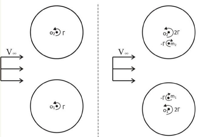
Figure 2: Staggered two cylinder problem of Crowdy (2006). Left: staggered cylinders with bound vortices. Right: vortex system with image vortices for the equivalent inverse point model.

3.1.4  Two circular cylinders with circulation

Crowdy (2006) gives a general theory which permits the calculation of lift for a finite number of staggered cylinders with bound vortex. Here we apply (31) to obtain the lift for his example of two vertically aligned cylinders (see Fig.2), both of radius $a=1/2$ and of given circulation $\Gamma_{1}=\Gamma_{2}=\Gamma$ ($\Gamma=-5,-2,0$), immersed in a uniform stream $V_{\infty}=1$ and placed at a distance $h\geq 1$ between their centers. The bound vortex associated with one cylinder has an image pair of two counter rotating vortices in the other, at the center and inverse point respectively. An image pair in one cylinder also has two counter rotating image vortices in the corresponding inverse points of the other cylinder, plus two cancelling images at the center of the other cylinder cancel. Thus in each cylinder, there are an infinite number of such inverse points, with counter rotating vortices of equal strength between any two adjacent inverse points, with distance becoming closer for newer generated images. If, for the $i$th cylinder,  the distance of the $k$th inverse point to the center of this cylinder is denoted as $h_{k}^{(i)}$, then

$$h_{1}^{(i)}h=a^{2}\text{, and }h_{k}^{(i)}\left(h-\frac{a^{2}}{h-h_{k-1}^{(i)}}\right)=a^{2}\text{ for }k>1$$ (32)

For an exact solution with  (31), we have to work with such infinite number of inverse points. Here we instead use an approximate method based on the remark that the inverse points in each cylinder are distributed in a narrow region. To see this, let $h_{k}^{(i)}=g^{(i)\text{ }}$ for $k\rightarrow\infty$, then by (32) we have $g^{(i)\text{ }}\left(h-\frac{a^{2}}{h-g^{(i)\text{ }}}\right)=a^{2}$, which can be solved to give

$$g^{(i)\text{ }}=\frac{1}{2}\left(h-\sqrt{h^{2}-4a^{2}}\right)$$ (33)

and one can verify that $a^{2}/h<h_{k}^{(i)}<g^{(i)\text{ }}$ for $k>1$. It can be further verified that the region between $y=a^{2}/h$ and $y=g^{(i)\text{ }}$ is very narrow even for $h$ close to $1$.

Hence within the framework of approximate solution we may merge all the inverse points into an equivalent one, with a distance $h_{e}^{(i)}$ to the center of the corresponding cylinder satisfying $a^{2}/h<h_{e}^{(i)}<g^{(i)\text{ }}$. Moreover, since these inverse points are denser close to $y=g^{(i)\text{ }}$, we just set $h_{e}^{(i)}=a^{2}/$$h$. With $a=\frac{1}{2}$, we have $h_{e}^{(i)}=h_{e}=0.5^{2}/h$.  Let $h_{ee}$ be the distance between the equivalent inverse points of the two cylinders, and $h_{eo}$ be the distance between the equivalent inverse point of one cylinder to the center of the other. Then

$$h_{ee}=h-2h_{e},\text{ \ }h_{eo}=h-h_{e}$$

With the approximation of equivalent inverse point, and considering the conservation of circulation, the vortex system in each cylinder can be simplified in the following way.

For the $1$st cylinder, there is one given bound vortex of circulation $\Gamma_{1}^{(b)}=\Gamma_{1}$ and one image vortex of circulation $\Gamma_{1}^{(o)}=\Gamma_{2}$ at the center of this cylinder, plus one equivalent image vortex of circulation $\Gamma_{1}^{(m)}=-\Gamma_{2}$ at the equivalent inverse point $y=h_{e}^{(i)}$. For the $2nd$ cylinder, this can be similarly defined. Moreover, each cylinder has a doublet of strength $\mu_{1}=\mu_{2}=\mu=2\pi a^{2}V_{\infty}=\frac{\pi}{2}$. There are also an infinite number of image doublets at the inverse points. When the equivalent inverse point is applied to the doublet, the strength of the doublet at this inverse point is $\mu_{1}^{(e)}=\mu_{2}^{(e)}=\mu^{(e)}\approx\mu a^{2}/h_{eo}^{2}$.

The velocities induced at the center and at the equivalent inverse points of the $1st$ and $2nd$ cylinders by the bound and image vortices and doublet of the $2nd$ and $1st$ cylinders are thus   

$$\left\{\begin{array}[]{c}u_{1}^{(o)}=-u_{2}^{(o)}=\frac{2\Gamma}{2\pi h}+\frac{-\Gamma}{2\pi h_{eo}}+\frac{\mu}{2\pi h^{2}}+\frac{\mu^{(e)}}{2\pi h_{eo}^{2}}\\ u_{1}^{(m)}=-u_{2}^{(m)}=\frac{2\Gamma}{2\pi h_{eo}}+\frac{-\Gamma}{2\pi h_{ee}}+\frac{\mu}{2\pi h_{eo}^{2}}+\frac{\mu^{(e)}}{2\pi h_{ee}^{2}}\end{array}\right.$$

The derivatives of the corresponding induced velocities are

$$\left\{\begin{array}[]{c}\frac{\partial u_{1}^{(\mu)}}{\partial y}=-\frac{\partial u_{2}^{(\mu)}}{\partial y}=\frac{2\Gamma}{2\pi h^{2}}+\frac{-\Gamma}{2\pi h_{eo}^{2}}+\frac{\mu}{\pi h^{3}}+\frac{\mu^{(e)}}{\pi h_{eo}^{3}}\\ \frac{\partial u_{1}^{(\sigma)}}{\partial y}=-\frac{\partial u_{2}^{(\sigma)}}{\partial y}=\frac{2\Gamma}{2\pi h_{eo}^{2}}+\frac{-\Gamma}{2\pi h_{ee}^{2}}+\frac{\mu}{\pi h_{eo}^{3}}+\frac{\mu^{(e)}}{\pi h_{ee}^{3}}\end{array}\right.$$

According to (31), the force formula for the lower airfoil is $L^{(1)}=L_{B}^{(1)}+L_{b}^{(1)}+L_{o}^{(1)}+L_{m}^{(1)}+L_{\mu}^{(1)}$ with $L_{B}^{(1)}=-\rho V_{\infty}\Gamma_{1}$, $L_{b}^{(1)}=-\rho u_{1}^{(o)}\Gamma_{1}$, $L_{o}^{(1)}=-\rho u_{1}^{(o)}\Gamma_{2}^{(o)}$, $L_{m}^{(1)}=-\rho u_{1}^{(m)}\Gamma_{2}^{(m)}$, $L_{\mu}^{(1)}=\rho\frac{\partial u_{1}^{(\mu)}}{\partial y}\mu_{1}$,$L_{\sigma}^{(1)}=\rho\frac{\partial u_{1}^{(\sigma)}}{\partial y}\mu^{(e)}$.

With $\rho=V_{\infty}=1$, $\Gamma_{1}=\Gamma_{2}^{(o)}=-\Gamma_{2}^{(m)}=\Gamma$ and $\mu_{1}=\mu=\frac{1}{2}\pi$, we have

$$L^{(1)}=-\Gamma-2u_{1}^{(o)}\Gamma+u_{1}^{(m)}\Gamma+\frac{\partial u_{1}^{(\mu)}}{\partial y}\mu+\frac{\partial u_{1}^{(\sigma)}}{\partial y}\mu^{(e)}$$

where the induced velocities $u_{1}^{(o)}$,$u_{1}^{(o)}$ and their derivatives $\partial u_{1}^{(\mu)}/\partial y,\partial u_{1}^{(\sigma)}/\partial y$ have been given above.   Similarly for the upper airfoil,

$$L^{(2)}=-\Gamma-2u_{2}^{(o)}\Gamma+u_{2}^{(m)}\Gamma+\frac{\partial u_{2}^{(\mu)}}{\partial y}\mu+\frac{\partial u_{2}^{(\sigma)}}{\partial y}\mu^{(e)}$$

The results, compared to Crowdy (2006), are displayed in Fig 3. We remark that the agreement is acceptable even when $h$ is short and despite the use of equivalent inverse point to merge all the inverse points. The short distance behavior, that is, there is an attraction force when the cylinders are close, has been discussed by Crowdy. Here it is found that this is due to the influence of the real and image doublets and the induced velocity gradient, described by $L_{\mu}$ and $L_{\sigma}$ in (31).  

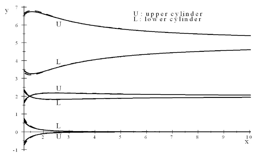
Figure 3: Comparison between the present result (solid lines) with Crowdy (2006, Fig.4)(dashed lines), for $\Gamma=0$ (lower),  $\Gamma=-2$ (middle) and $\Gamma=-5$ (upper). Dashed lines: Crowdy.

3.2 Karman vortex street

The problem of the Karman vortex street behind a bluff body (Fig.4) is rather special since the shape of the body is unknown. Hence we can only use the singularity velocity method to study the drag. The Karman vortex street is a double row of staggered and counter-rotating vortices of strength $\Gamma>0$ and $\Gamma<0$ and moving horizontally at speed

$$V=\frac{\Gamma\pi}{a}\tanh\frac{\pi b}{a}$$

Here $b$ is the vertical separation distance between these two rows and $a$ is the horizontal separation distance between adjacent two vortices in each row (see for instance Milne-Thomson 1968,p377). The period of vortex shedding in each row is thus

$$\tau=\frac{a}{V_{\infty}-V}$$

According to (30), the drag, averaged over $\tau$, due to the shedding of new vortex pair, separated at a distance $\widetilde{y}_{n}-y_{n}=b$, is

$$D_{u}=\rho\frac{1}{\tau}\int_{0}^{\tau}\frac{d\Gamma_{n}\left(\widetilde{y}_{n}-y_{n}\right)dt}{dt}=\frac{\rho\ }{\tau}\int_{0}^{\tau}d\left(\Gamma_{n}\left(\widetilde{y}_{n}-y_{n}\right)\right)=\frac{\rho b\Gamma}{\tau}$$

When the expressions for $V$ and $\tau$ are used, we obtain

$$D_{u}=\frac{\rho b\Gamma\left(V_{\infty}-V\right)}{a}=\frac{\rho b\Gamma}{a}\left(V_{\infty}-\frac{\Gamma\pi}{a}\tanh\frac{\pi b}{a}\right)$$

This is the well-known formula for the unsteady part of the drag, which has been otherwise obtained by sophisticate Blasius approach (Milne-Thomosn 1968,p382), impulse approach (Saffman 1992,p 137) or integral approach (Howe,1995,p417). The way to obtain this force using the present approach appears to be much easier.

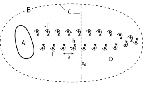
Figure 4: Control volume for the Karman Vortex street problem. A cutline $x=x_{d}$ separates the flow regime into an upstream part and a downstream part (D).

Remark also that, apart from the drag component $D_{u}$ due to shedding of new vortices, there is also another component $D_{s}$ due to quasi steady flow formed by two rows of periodically counter-rotating vortices spreading infinitely into the downstream direction. No existing force formula, including the present formula (12), can be directly applied to this case. One then needs to construct a special downstream boundary and relates this component of drag to the momentum flux across this boundary. For details, see Milne-Thomosn(1968,p382), (Saffman 1992,p 137) and Howe (1995,p417), where different ways for setting the downstream boundary are used.  Let $x=x_{d}$ be such a boundary downstream of the body and intersecting the vortex street in its uniform region. Let $(u_{k},v_{k})$ be the induced velocity by the vortex street. Then, in Appendix B, we shall prove that, the use of (12) leads to

$$D_{s}=\frac{1}{2}\rho\int_{x=x_{d}}\left(u_{k}^{2}-v_{k}^{2}\right)dy$$ (34)

which is exactly the same as obtained by Howe (1995, Eq.(5.11)) through an integral approach. Howe then shows that (34) yields

$$D_{s}=\frac{\Gamma^{2}}{2a^{2}}\left(\frac{a}{\pi}-b\tanh\frac{\pi b}{a}\right)$$

The total drag $D=D_{u}+D_{s}$ is thus

$$D=\frac{\rho b\Gamma\left(V_{\infty}-V\right)}{a}+\frac{\Gamma^{2}}{2a^{2}}\left(\frac{a}{\pi}-b\tanh\frac{\pi b}{a}\right)$$

3.3 Interaction of a thin airfoil with outside vortices

Consider a thin airfoil without thickness, for which the camber line is defined by

$$y=y_{a}(x)=-\alpha x+f(x),0<x<c_{A}$$ (35)

Here $\alpha$ is the angle of attack and $f(x)$ is small with respect to $c_{A}$. The upstream inflow is assumed horizontal. First we need to find the distribution of vortices. Then we apply both (25) (singularity velocity method) and (26) (induced velocity method) to obtain the force formulas. The results will be validated through the problem of Wagner with vortex shedding. Finally the interaction of the airfoil with another one, represented by a bound vortex, is studied.

3.3.1 Method of solution

To solve this problem we assume a distribution of vorticity $\gamma(x)$ on the airfoil so that the velocity at any point on the airfoil is

$$u_{A}(x) = V_{\infty}-\displaystyle\int\limits_{0}^{c_{A}}\frac{\gamma(\xi)(y-y_{a}(\xi))d\xi}{2\pi\left((x-\xi)^{2}+(y-y_{a}(\xi))^{2}\right)}+u_{v}(x)\approx V_{\infty}+u_{v}(x)$$

$$v_{A}(x) = \displaystyle\int\limits_{0}^{c_{A}}\frac{\gamma(\xi)(x-\xi)d\xi}{2\pi\left((x-\xi)^{2}+(y-y_{a}(\xi))^{2}\right)}+v_{v}(x)\approx\displaystyle\int\limits_{0}^{c_{A}}\frac{\gamma(\xi)d\xi}{2\pi(x-\xi)}+v_{v}(x)$$

where $(u_{v}(x),v_{v}(x))$ is the velocity on the airfoil induced by vortices outside of the airfoil and is the only correction to the standard method for thin airfoil theory (Anderson 2010). Substituting the expressions of $u_{A}(x)$ and $v_{A}(x)$  into the boundary condition

$$\frac{v_{A}}{u_{A}}=-\alpha+\frac{df(x)}{dx}$$

we obtain the equation for $\gamma(x)$,

$$\int\limits_{0}^{c_{A}}\frac{\gamma(\xi)d\xi}{2\pi(x-\xi)}=V_{\infty}\left(\frac{df(x)}{dx}-\alpha+g(x)\right)\text{\ }$$

where the function

$$g(x)=\frac{u_{v}(x)}{V_{\infty}}\left(\frac{df(x)}{dx}-\alpha\right)-\frac{v_{v}(x)}{V_{\infty}}$$

is due to the induction by the outside vortices. The standard thin airfoil theory is recovered if $g(x)=0$. Let $x=\frac{c_{A}}{2}\left(1-\cos\theta\right),\xi=\frac{c_{A}}{2}\left(1-\cos\beta\right)$ for $0<\theta,\beta<\pi$, then $\gamma(x)$ can be expressed as

$$\gamma(\theta)=2V_{\infty}\left(A_{0}\frac{1+\cos\theta}{\sin\theta}+\sum_{n=1}^{n=\infty}A_{n}\sin\left(n\theta\right)\right)$$ (36)

with    

$$\left\{\begin{array}[]{l}A_{0}=-\alpha+\frac{1}{\pi}\int_{0}^{\pi}\frac{df(\xi)}{d\xi}d\beta+a_{0}\\ A_{n,n>1}=-\frac{2}{\pi}\int_{0}^{\pi}\frac{df(\xi)}{d\xi}\cos\left(n\beta\right)d\beta+a_{n}\end{array}\right.$$ (37)

where the coefficients

$$\left\{\begin{array}[]{l}a_{0}=-\frac{1}{\pi V_{\infty}}\int_{0}^{\pi}\left(v_{v}(\xi)-u_{v}(\xi)\left(\frac{df(\xi)}{d\xi}-\alpha\right)\right)d\beta\\ a_{n,n>1}=\frac{2}{\pi V_{\infty}}\int_{0}^{\pi}\left(v_{v}(\xi)-u_{v}(\xi)\left(\frac{df(\xi)}{d\xi}-\alpha\right)\right)\cos\left(n\beta\right)d\beta\end{array}\right.$$ (38)

are due to the outside vortices, and the remaining parts in $A_{0},A_{n}$ are given by the classical thin airfoil theory.

Remark that in the case of a thin airfoil with thickness, we may add, in addition to the vorticity distribution $\gamma(x)$, a distribution of source doublet $\mu(x)$ on the camber line. Then the boundary conditions should be defined for both the upper and lower surfaces of the airfoil which will provide us the necessary conditions to determine both $\gamma(x)$ and $\mu(x)$.

To find $(u_{v}(x),v_{v}(x))$ the position of each outside vortex $(i)$ must be determined, through solving the equations

$$\left\{\begin{array}[]{l}\frac{dx_{i}}{dt}=V_{\infty}-\displaystyle\int\limits_{0}^{c_{A}}\frac{\gamma(\xi)(y_{i}-y_{a}(\xi))d\xi}{2\pi\left((x_{v}-\xi)^{2}+(y_{v}-y_{a}(\xi))^{2}\right)}-\displaystyle\sum\limits_{j,j\neq i}\frac{\Gamma_{j}(\xi)(y_{i}-y_{j})d\xi}{2\pi\left((x_{i}-x_{j})^{2}+(y_{i}-y_{j})^{2}\right)}\\ \frac{dy_{i}}{dt}=\displaystyle\int\limits_{0}^{c_{A}}\frac{\gamma(\xi)(x_{i}-\xi)d\xi}{2\pi\left((x-\xi)^{2}+(y-y_{a}(\xi))^{2}\right)}+\displaystyle\sum\limits_{j,j\neq i}\frac{\Gamma_{j}(\xi)(x_{i}-x_{j})d\xi}{2\pi\left((x_{i}-x_{j})^{2}+(y_{i}-y_{j})^{2}\right)}\end{array}\right.$$ (39)

3.3.2 Lift force by the singularity velocity method

The lift force in the form (25) can be rewritten here as

$$L=-\rho V_{\infty}\int_{0}^{c_{A}}\gamma dx+\rho\frac{d}{dt}\int_{0}^{c_{A}}\gamma xdx+L_{out}$$

where $L_{out}$ is due to the outside vortices. For point vortices of circulation $\Gamma_{i}$

$$L_{out}=-\rho\sum_{i}\left(V_{\infty}-\frac{d\left(\Gamma_{i}x_{i}\right)}{dt}\right)$$

and for a distribution of outside vortices of strength $k$

$$L_{out}=-\rho V_{\infty}\int\int_{ou}kdxdy+\rho\frac{d}{dt}\int\int_{ou}kxdxdy$$ (40)

With $\gamma(x)$ in the form (36), we get for the circulation of bound vortex

$$\Gamma_{b}=\int_{0}^{c_{A}}\gamma dx=\pi c_{A}V_{\infty}\left(A_{0}+\frac{1}{2}A_{1}\right)$$ (41)

and the moment of inner vortices   

$$\int_{0}^{c_{A}}\gamma xdx = \frac{V_{\infty}c_{A}^{2}}{2}\int_{0}^{\pi}\left(A_{0}\frac{1+\cos\theta}{\sin\theta}+\sum_{n=1}^{n=\infty}A_{n}\sin\left(n\theta\right)\right)\left(1-\cos\theta\right)\sin\theta d\theta$$

$$= \frac{\pi V_{\infty}c_{A}^{2}}{4}\left(A_{0}+A_{1}-\frac{1}{2}A_{2}\right)$$

Thus the formula for the lift force is

$$L=-\rho V_{\infty}\Gamma_{b}+L_{int}+L_{out}$$ (42)

where

$$L_{int}=\frac{\pi\rho V_{\infty}c_{A}^{2}}{4}\frac{d}{dt}\left(A_{0}+A_{1}-\frac{A_{2}}{2}\right)$$ (43)

When the outside vortices are given and when $f(\xi)$ and $\alpha$ are known,  the formulas (37) and (38) with $\xi=\frac{c_{A}}{2}\left(1-\cos\beta\right)$ yield the required coefficients $A_{0}$, $A_{1}$ and $A_{2}$.

3.3.3 Lift force by the induced velocity method

If we use (26) then

$$L=-\rho V_{\infty}\int_{0}^{c_{A}}\gamma dx-\rho\int_{0}^{c_{A}}\widetilde{u}\gamma dx+\rho\frac{d}{dt}\int_{0}^{c_{A}}\gamma xdx+L_{p}$$

where $\int_{0}^{c_{A}}\gamma xdx=\frac{\pi V_{\infty}c_{A}^{2}}{4}\left(A_{0}+A_{1}-\frac{1}{2}A_{2}\right)$ as above,  $L_{p}=\rho\sum x_{s}\frac{d\Gamma_{s}}{dt}$  is due to vortex production outside of the airfoil (that due to vortex production inside the body is included in the third term on the right hand side).

Assume that for the present problem, vortex is shed only at the trailing edge, so that $x_{s}=c_{A},\frac{d\Gamma_{s}}{dt}=\frac{d}{dt}\int\int_{ou}kdxdy=-\ \frac{d\Gamma_{b}}{dt}$, and

$$L_{p}=-\rho c_{A}\frac{d\Gamma_{b}}{dt}$$

Moreover, since the vortex sheet, inducing $\widetilde{u}$, is on the horizontal line downstream of the plate, $\int_{0}^{c_{A}}\widetilde{u}\gamma dx\approx 0$, and thus

$$L=-\rho V_{\infty}\Gamma_{b}-\rho\int_{0}^{c_{A}}\widetilde{u}\gamma dx+\frac{\pi\rho V_{\infty}c_{A}^{2}}{4}\frac{d}{dt}\left(A_{0}+A_{1}-\frac{A_{2}}{2}\right)-\rho c_{A}\frac{d\Gamma_{b}}{dt}$$ (44)

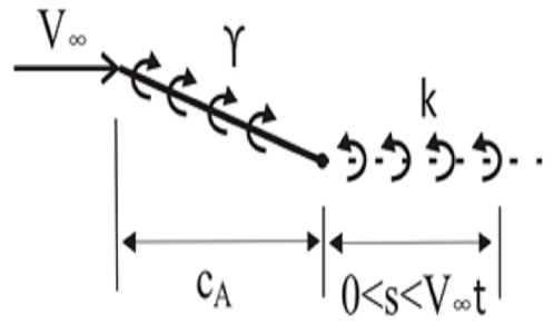
Figure 5: Impulsively started plate with vortex shedding

3.3.4 Wagner problem for impulsively starting plate

Consider a flat plate of length $c_{A}$ at small incidence $\alpha$, impulsively set into motion with constant velocity $V_{\infty}$ (Fig.5). At a distance $s$ from the trailing edge, a vortex sheet of strength $k(s,t)$ spreading over $0<s<V_{\infty}t$ and satisfying $\frac{Dk}{Dt}=\frac{\partial k}{\partial t}+V_{\infty}\frac{\partial k}{\partial x}=0$ under the assumption of negligible self-induced motion. Moreover, since the total circulation is conserved, that is $\Gamma_{b}+\int_{0}^{V_{\infty}t}k(s,t)ds=0$, we may use (41) to write the relation for determining $k(s,t)$

$$\int_{0}^{V_{\infty}t}k(s,t)ds+\pi c_{A}V_{\infty}\left(A_{0}+\frac{1}{2}A_{1}\right)=0$$ (45)

In Appendix C we shall prove that

$$A_{0}+\frac{1}{2}A_{1}=-\alpha-\frac{1}{\pi V_{\infty}c_{A}}\int_{0}^{V_{\infty}t}\left(1-\frac{\sqrt{c_{A}+s}}{\sqrt{s}}\right)k(s,t)ds$$ (46)

Inserting (46) into (45), we obtain the required equation for $k(s,t)$

$$\int_{0}^{V_{\infty}t}\frac{\sqrt{c_{A}+s}}{\sqrt{s}}k(s,t)ds=\pi c_{A}V_{\infty}\alpha$$ (47)

which is exactly the same as given by the method of conformal mapping, see for instance Saffman (1992,p111,eq (8)).

In Appendix C we also show that

$$A_{0}+A_{1}-\frac{1}{2}A_{2}=-\alpha-\frac{1}{\pi V_{\infty}}\int_{0}^{V_{\infty}t}H(s)k(s,t)ds$$

where $H(s)=\frac{4}{c_{A}^{2}}\left(s-\sqrt{sc_{A}+s^{2}}\right)-\frac{2}{c_{A}}\frac{\sqrt{c_{A}+s}}{\sqrt{s}}+\frac{4}{c_{A}}$.  Using (47) we may further write

$$A_{0}+A_{1}-\frac{1}{2}A_{2}=\alpha-\frac{4}{\pi V_{\infty}c_{A}}\int_{0}^{V_{\infty}t}k(s,t)ds-\frac{4}{\pi V_{\infty}c_{A}^{2}}\int_{0}^{V_{\infty}t}\left(s-\sqrt{sc_{A}+s^{2}}\right)k(s,t)ds$$ (48)

  

For the singularity velocity method, the component $L_{int}$ defined by (43) now becomes

$$L_{int}=-\rho c_{A}\frac{d}{dt}\int_{0}^{V_{\infty}t}k(s,t)ds-\rho\frac{d}{dt}\int_{0}^{V_{\infty}t}\left(s-\sqrt{sc_{A}+s^{2}}\right)k(s,t)ds$$

when (48) is used, and $L_{out}$ by (40)  becomes

$$L_{out}=-\rho V_{\infty}\int_{0}^{V_{\infty}t}k(s,t)ds+\rho\frac{d}{dt}\int_{0}^{V_{\infty}t}k(s,t)\left(c_{A}+s\right)ds$$

Inserting these into the force formula (42) and making use of $\Gamma_{b}+\int_{0}^{V_{\infty}t}k(s,t)ds=0$, we obtain

$$L=\rho\frac{d}{dt}\int_{0}^{V_{\infty}t}\sqrt{sc_{A}+s^{2}}k(s,t)ds$$ (49)

For the induced velocity method, inserting (48) into the force formula (44)  and remarking that $\int_{0}^{c_{A}}\widetilde{u}\gamma dx\approx 0$ since the vortex sheet, inducing $\widetilde{u}$, is on the horizontal line downstream of the plate, we get

$$L=-\rho V_{\infty}\Gamma_{b}-\ \left(\rho c_{A}\frac{d}{dt}\int_{0}^{V_{\infty}t}k(s,t)ds+\ \rho\frac{d}{dt}\int_{0}^{V_{\infty}t}\left(s-\sqrt{sc_{A}+s^{2}}\right)k(s,t)ds\right)-\rho c_{A}\frac{d\Gamma_{b}}{dt}$$

which, when $\Gamma_{b}=-\int_{0}^{V_{\infty}t}k(s,t)ds$ is used, yields

$$L=-\rho V_{\infty}\Gamma_{b}-\ \ \rho\frac{d}{dt}\int_{0}^{V_{\infty}t}\left(s-\sqrt{sc_{A}+s^{2}}\right)k(s,t)ds$$ (50)

The force formula (50) based on the singularity velocity method and that (49) based on the induced velocity are in fact identical since it can be shown that

$$V_{\infty}\Gamma_{b}+\ \ \frac{d}{dt}\int_{0}^{V_{\infty}t}sk(s,t)ds=0$$ (51)

The identity (51) will be proved below just for small time.

Now we use (50) to study the lift for two extreme case, $t\rightarrow$${\normalsize\infty}$ and $t\rightarrow 0$. For $t\rightarrow$${\normalsize\infty}$, Saffman (1992,p114) shows that

$$\frac{d}{dt}\int_{0}^{V_{\infty}t}\left(s-\sqrt{sc_{A}+s^{2}}\right)k(s,t)ds=0$$

Hence, by (50),

$$L=L_{\infty}=-\rho V_{\infty}\Gamma_{b}(\infty)$$

where $\Gamma_{b}(\infty)=\pi V_{\infty}c_{A}\alpha$ is the steady state circulation.

For small time $t\rightarrow 0$, we may write $\left(s-\sqrt{sc_{A}+s^{2}}\right)$$\rightarrow$$\sqrt{sc_{A}}$, thus by (50),

$$L\approx-\rho V_{\infty}\Gamma_{b}+\ \ \rho\frac{d}{dt}\int_{0}^{V_{\infty}t}\sqrt{sc_{A}}k(s,t)ds$$

Furthermore, it can be straightforwardly verified that the solution for (47) satisfying $\frac{Dk}{Dt}=0$ in addition is

$$k(s,t)\approx\frac{V_{\infty}\alpha\sqrt{c_{A}}}{\sqrt{V_{\infty}t-s}},t\rightarrow 0$$

and thus

$$\Gamma_{b}=-\int_{0}^{V_{\infty}t}k(s,t)ds=-2V_{\infty}\alpha\sqrt{c_{A}}\sqrt{V_{\infty}t}\text{, }\int_{0}^{V_{\infty}t}sk(s,t)ds\ =V_{\infty}\alpha\sqrt{c_{A}}\frac{4\left(V_{\infty}t\right)^{\frac{3}{2}}}{3}$$

Due to the above expressions, (51) obviously holds.

Now for small time, it holds that , $\Gamma_{b}\rightarrow 0$, thus

$$L\approx\rho\frac{d}{dt}\int_{0}^{V_{\infty}t}\sqrt{sc_{A}}k(s,t)ds\approx\rho c_{A}V_{\infty}\alpha\frac{d}{dt}\int_{0}^{V_{\infty}t}\frac{\sqrt{s}}{\sqrt{V_{\infty}t-s}}ds$$

Let $S=\sqrt{s}$, then

$$\int\frac{\sqrt{s}}{\sqrt{V_{\infty}t-s}}ds=2\int\frac{S^{2}}{\sqrt{V_{\infty}t-S^{2}}}dS=-S\sqrt{V_{\infty}t-S^{2}}+V_{\infty}t\arcsin\frac{S}{\sqrt{V_{\infty}t}}+C$$

Hence $\int_{0}^{V_{\infty}t}\frac{\sqrt{s}}{\sqrt{V_{\infty}t-s}}ds=\frac{\pi V_{\infty}t}{2}$ and therefore

$$L=\frac{1}{2}\pi\rho V_{\infty}^{2}c_{A}\alpha$$

Thus we recover the well-known result that for a flat plate impulsively generated, the initial lift on the plate is only one-half of the final lift $L_{\infty}=\pi\rho V_{\infty}^{2}c_{A}\alpha$.  Note also that the initial lift for airfoils with thickness has also been studied, see Chow& Huang (1982) and Graham (1983).

3.3.5 A bound vortex above a flat plate

The lift for an airfoil with a free line vortex over the airfoil has been studied, for instance by Saffman&Shefield (1977) using the method of conformal mapping. There is a condition for the vortex strength such that the free vortex is standing. First we apply the present theory to this case to provide another validation against known results. Then we replace this free vortex by a bound vortex, to find the force due to interaction between a flat plate with another airfoil represented by a lumped vortex.

Consider an outside vortex of strength $\Gamma_{v}>0$ at a distance $h$ above the midpoint ($x_{m}=\frac{c_{A}}{2}$) of a flat plate of length $c_{A}=2a$ parallel to a stream of velocity $V_{\infty}$ (Fig.6) .  The formulas (37) and (38) now reduce to

$${\normalsize A_{0}=-\frac{1}{\pi V_{\infty}}\int_{0}^{\pi}v_{v}(\xi)d\beta}\text{, }{\normalsize\ A_{n,n>1}=\frac{2}{\pi V_{\infty}}\int_{0}^{\pi}v_{v}(\xi)\cos\left(n\beta\right)d\beta}$$

Denote $\overline{h}=\frac{h}{\frac{1}{2}c_{A}}$. With $v_{v}(\xi)$ given by

$$v_{v}(\xi)=\frac{\Gamma_{v}}{2\pi}\frac{\xi-x_{m}}{(\xi-x_{m})^{2}+h^{2}}=-\frac{\Gamma_{v}}{2\pi x_{m}}\frac{\cos\beta}{\cos^{2}\beta+\overline{h}^{2}},$$

we get $A_{0}=A_{2}=0$ and

$$A_{1}=-\frac{2\Gamma_{v}}{\pi V_{\infty}c_{A}}\left(1-\frac{\overline{h}}{\sqrt{1+\overline{h}^{2}}}\right)=-\frac{2\Gamma_{v}}{\pi V_{\infty}c_{A}}\Upsilon(\overline{h})\left(\sqrt{1+\overline{h}^{2}}+\overline{h}\right)$$ (52)

where

$$\Upsilon(\overline{h})=\left(\sqrt{1+\overline{h}^{2}}+\overline{h}\right)^{-2}\left(1+\overline{h}^{2}\right)^{-\frac{1}{2}}$$ (53)

Hence, with (36) and (41), we obtain $\gamma(\theta)=2V_{\infty}A_{1}\sin\theta$ and

$$\Gamma_{b}=-\Upsilon(\overline{h})\left(\sqrt{1+\overline{h}^{2}}+\overline{h}\right)\Gamma_{v}$$ (54)

This condition holds independent of whether the vortex is free or bounded.

A) Free vortex case.  Apply (39) to the present case, and with $\gamma(\beta)=2V_{\infty}A_{1}\sin\beta$, we obtain the velocity of the vortex (if it is free)

$$\frac{dx_{v}}{dt}=V_{\infty}+\frac{2\Upsilon(\overline{h})\Gamma_{v}}{\pi c_{A}}\text{, \ }\frac{dy_{v}}{dt}=0$$

Set $\frac{dx_{v}}{dt}=0$, we obtain

$$\Gamma_{v}=-\frac{\pi V_{\infty}c_{A}}{2\Upsilon(\overline{h})}$$ (55)

The method of singularity approach (42) gives a lift $L=-\rho V_{\infty}\Gamma_{b}-\rho\left(V_{\infty}-\frac{dx_{v}}{dt}\right)\Gamma_{v}$, and since  $\frac{dx_{v}}{dt}=0$, we have    

$$L=\rho V_{\infty}\left(\Upsilon(\overline{h})\left(\sqrt{1+\overline{h}^{2}}+\overline{h}\right)-1\right)\Gamma_{v}$$ (56)

Thus if $\Gamma_{v}$ is given by (55) and $\Gamma_{b}$ is given by (54), then the outside vortex will be stationary and the lift is given by (56). This result is exactly the same as given by  the method of conformal mapping (cf. Saffman1992,p122).

B) Bound vortex case. This is a multibody case, though the body above the plate is represented by a bound vortex. The force formula (44) (induced velocity method) applied here gives

$$L=-\rho V_{\infty}\Gamma_{b}-\rho\int_{0}^{c_{A}}\widetilde{u}\gamma dx$$ (57)

Here

$$\widetilde{u}=u_{v}(\xi)=\frac{\Gamma_{v}}{2\pi}\frac{h}{(\xi-x_{m})^{2}+h^{2}}=\frac{\Gamma_{v}}{2\pi x_{m}}\frac{\overline{h}}{\cos^{2}\beta+\overline{h}^{2}}$$

is the velocity in the airfoil induced by the outside bound vortex. With $\gamma(\beta)=2V_{\infty}A_{1}\sin\beta$ and with $A_{1}$ given by (52), we have

$$\int_{0}^{c_{A}}\widetilde{u}\gamma dx=\frac{\Gamma_{v}V_{\infty}A_{1}\overline{h}}{\pi}\int_{0}^{\pi}\frac{\sin\beta\sin\beta}{\cos^{2}\beta+\overline{h}^{2}}d\beta=-\frac{2\Upsilon(\overline{h})\Gamma_{v}^{2}}{c_{A}}$$ (58)

since

$${\normalsize\displaystyle\int\limits_{0}^{\pi}\frac{\sin\beta\sin\beta d\beta}{\cos^{2}\beta+\overline{h}^{2}}=-\pi+\frac{\overline{h}^{2}+1}{\overline{h}\sqrt{1+\overline{h}^{2}}}\pi.}$$

Inserting (58) and (54) into (57) we obtain finally

$$L=\rho V_{\infty}\Upsilon(\overline{h})\left(\sqrt{1+\overline{h}^{2}}+\overline{h}\right)\Gamma_{v}+\rho\frac{2\Upsilon(\overline{h})\Gamma_{v}^{2}}{c_{A}}$$ (59)

Remark 3.1. The formula (59) with $\Upsilon(\overline{h})$ defined by (53) gives the lift of a horizontal flat plate with another airfoil of any given circulation $\Gamma_{v}$ and at a distance $h$ above the middle point of the plate, provided the additional airfoil is simplified as a lumped vortex.

Remark 3.2. When, in addition, the circulation $\Gamma_{v}$ satisfies (55), then it is clear that (59) gives exactly the same force as (56). This is because that when (55) is satisfied, the vortex is standing for the free vortex case so that we shall have the same force as for a bound vortex.

Define the lift coefficient as $c_{l}=2L/\rho V_{\infty}^{2}c_{A}$ and the normalized vortex strength as $\overline{\Gamma}_{v}=\overline{\Gamma}_{v}/V_{\infty}c_{A}$, we obtain from (59) the lift coefficient for the flat plate

$$c_{l}=2\left(\sqrt{1+\overline{h}^{2}}+\overline{h}+2\overline{\Gamma}_{v}\right)\Upsilon(\overline{h})\overline{\Gamma}_{v}$$

The lift coefficient as a function of $\overline{h}$ for $\overline{\Gamma}_{v}=-1$ and $\overline{\Gamma}_{v}=1$ is displayed in Fig 6. When the upper vortex has a clockwise circulation ($\overline{\Gamma}_{v}=-1$), the lift of the airfoil, produced by interaction, is negative for $\sqrt{1+\overline{h}^{2}}+\overline{h}<-2\overline{\Gamma}_{v}$ or $\overline{h}<\frac{3}{4}$, and positive for $\overline{h}>\frac{3}{4}$. Hence there is a distance at which the flat plate has no lift gain from the upper vortex. When the upper vortex has anticlockwise circulation ($\overline{\Gamma}_{v}=1$), the lift is always positive.

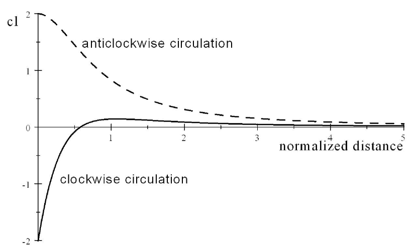
Figure 6: Lift coefficient of the flat plate, which is interaction with a bound vortex at $\overline{h}$ above the middle point of the plate.

4 Summary

Started from a momentum balance analysis, and proceeded with inter exchange between the singularity velocity and induced flow velocity, we have obtained force formulas in both singularity form ( see (12) for method of singularity velocity, and (19) or (24) for single body or multibody method of induced velocity) and integral form  (see (25) for method of singularity velocity and (26) for multibody method of induced velocity), for which bound singularities, multiple free singularities and multiple bodies can be considered. The influence of the adjacent bodies on the actual body can be simply treated as influence of singularities representing the adjacent bodies, in a similar way as free singularities. Moreover, the influence on the force by vortex production is treated in a simple and explicit way (see (23) and (28), or Remark 2.2 in section 2.6).

The present work is new for four reasons. First, it covers the work of Wu, Yang &Young (2012) as a special case, and includes in addition the effect of bound vortices and vortex production (see Remark 2.3 in section 2.6). Second, the way to obtain the force formulas is based on the interaction of various singularities, and thus is useful for explicitly interpreting the influence due to various resources. For instance, we have shown that the interaction between free singularities do not contribute to forces, while the induced velocity effect is due to interaction between free singularities and inner singularities (see section 2.3). Third, the present result includes the situation where the discrete singularities are replaced by a distribution of vortices and source doublets, thus we have an integral approach which, without the use of an auxiliary function, gives individual forces for each body in the case of multiple bodies (see section 2.5). Last, the present study appears to provide a bridge between the singularity velocity approach, induced velocity approach and some integral approaches.

The present results appear to be useful for deriving analytical force formulas even when multibody is considered. The validation study presented in section 3 demonstrates that analytical force formulas can be obtained even for rather complex problems. The example for an airfoil on top of which there is another airfoil (actually represented by a bound vortex) shows that it is possible to use the present method to derive analytical interaction forces for multiple airfoils, and this will be for a future study.

The present results are actually restricted to two dimensional inviscid flow. For viscous flow it appears that the viscous effect can be treated separately, by simply adding an additional boundary integral (Howe 1995).  Moreover, we did not consider the influence of body deformation, for which well established theories exist (Landweber&Miloh 1980, Howe 1995, Kanso&Oskouei 2008). Finally, the case with body acceleration and rotation has not been tested in this paper. These problems need further studies.

Similar analysis for axisymmetric flow has been carried out for insect flights (Wang&Wu 2010, Wang&Wu,2012), for which the influence of free vortices (in the form of vortex rings, or axisymmetric Karman vortex street) and insect body on the lift produced by the flapping wing is related to the induced velocity. In these studies the influence of the speeds of image vortices has been neglected, hence requiring further studies.

Appendix A Momentum change inside a fixed body

Now will show that

$$L_{a}\doteq\frac{d}{dt}\int\int_{A}\rho vdydx=0\text{, }D_{a}\doteq\frac{d}{dt}\int\int_{A}\rho udydx=0$$ (60)

when the body $A$ is considered fixed.

For each vortex or source $i$ inside the body,  we define an infinitesimal fixed circle of radius $r_{t}\triangleq\sqrt{(x-x_{i})^{2}+(y-y_{i})^{2}}=\varepsilon$ whose center instantaneously coincides with the vortex. For convenience we use here the subscript $x,y$ and $t$ denote the partial differentials with respect to $x$,$y$ and $t$. Let $\Sigma$ be the region bounded by the contour of the body $\partial A$ and the circumferences of the circles $r_{i}=\varepsilon$. Below are some additional relations.

Decompose $L_{a}$ defined in (60) as

$$L_{a}=\text{\ \ }\rho\frac{d}{dt}\int\int_{\Sigma}vdydx+\rho\sum_{i,in}\frac{d}{dt}\int\int_{r_{i}<\varepsilon}vdydx\text{\ }$$

Since $v=-\psi_{x}$ and since $\psi$ is analytical in $\Sigma$, we use the divergence theorem to write

$$\int\int_{\Sigma}vdydx=-\int\int_{\Sigma}\psi_{x}dydx=-\oint\limits_{\partial A}\psi dy+\sum_{i,in}\oint\limits_{r_{i}=\varepsilon}\psi dy$$

Hence

$$L_{a}=-\frac{d}{dt}\oint\limits_{\partial A}\psi dy+\sum_{i,in}\frac{d}{dt}\oint\limits_{r_{i}=\varepsilon}\psi dy+\rho\sum_{i,in}\frac{d}{dt}\int\int_{r_{i}<\varepsilon}vdydx$$

Consider the last term on the right hand side. Across an element of length $r_{i}d\theta_{i}$ at $(r_{i},\theta_{i})$ on the circumference of the circle $r_{i}<\varepsilon$, the loss of momentum due to the movement of the vortex $(i)$ is

$$dm_{i}=-v^{(i)}\left(x_{i,t}\cos\theta_{i}+y_{i,t}\sin\theta_{i}\right)r_{i}d\theta_{i}$$

Remark that $v^{(i)}=\frac{\Gamma_{i}\cos\theta_{i}}{2\pi r_{i}}$  and

$$\frac{d}{dt}\int\int_{r_{i}<\varepsilon}vdydx=\sum_{i,in}\int_{0}^{2\pi}dm_{i}=-\sum_{i,in}\frac{\Gamma_{i}}{2\pi}\int_{0}^{2\pi}\cos\theta_{i}\left(x_{i,t}\cos\theta_{i}+y_{i,t}\sin\theta_{i}\right)d\theta_{i}$$

Hence

$$\sum_{i,in}\frac{d}{dt}\int\int_{r^{(i)}<\varepsilon}vdydx=-\sum_{i,in}\frac{\Gamma_{i}}{2}x_{i,t}$$

If sources can be similarly analyzed.  When both vortices and sources are present we may write

$$\sum_{i,in}\frac{d}{dt}\int\int_{r^{(i)}<\varepsilon}vdydx=-\sum_{i,in}\left(\frac{\Gamma_{i}}{2}x_{i,t}-\frac{m_{i}}{2}y_{i,t}\right)$$

Now consider the second term on the right hand side. First consider vortices.

$$\psi_{t}^{(i)}=-\frac{\partial}{\partial t}\left(\frac{\Gamma_{i}}{2\pi}\ln r_{i}\right)=-\frac{\Gamma_{i}}{2\pi r_{i}}r_{i,t}$$

Let $\left(x,y\right)$ be a fixed point on the circle. Differentiating $x-x_{i}=r_{i}\cos\theta_{i}$ and $y-y_{i}=r_{i}\sin\theta_{i}$ with respect to time we obtain

$$r_{i}\theta_{i,t}=x_{i,t}\sin\theta_{i}-y_{i,t}\cos\theta_{i}\text{, \ }r_{i,t}=-x_{i,t}\cos\theta_{i}-y_{i,t}\sin\theta_{i}$$

Remark also that $\int_{0}^{2\pi}\cos^{2}\theta^{(i)}d\theta^{(i)}=\pi$ and $\int_{0}^{2\pi}\cos\theta^{(i)}\sin\theta^{(i)}d\theta^{(i)}=0$. Thus and similarly we have

$$\oint\limits_{r_{i}=\varepsilon}\psi_{i,t}dy=-\frac{\Gamma_{i}}{2\pi}\int_{0}^{2\pi}r_{i,t}\cos\theta_{i}d\theta_{i}=\frac{\Gamma_{i}}{2}x_{i,t}$$

Hence

$$\sum_{i,in}\frac{d}{dt}\oint\limits_{r_{i}=\varepsilon}\psi dy=\sum_{i,in}\frac{\Gamma_{i}}{2}x_{i,t}$$ (61)

When sources are included, the analysis is similar and we may write

$$\sum_{i,in}\frac{d}{dt}\oint\limits_{r_{i}=\varepsilon}\psi dy=\sum_{i,in}\left(\frac{\Gamma_{i}}{2}x_{i,t}-\frac{m_{i}}{2}y_{i,t}\right)$$

In summary we have proved

$$L_{a}=-\frac{d}{dt}\oint\limits_{\partial A}\psi dy$$

Since here the body is assumed stationary so that $\psi$ is a constant along the body, and thus $\oint\limits_{\partial A}\psi dy=0$. This means $L_{a}=0.$

Similarly we may prove $D_{a}=0.$

Appendix B Additional expression for Karman vortex street

To prove (34) using the present force formula (12),  we need a relation between the velocities of the inner and outer vortices. For this purpose will define a large contour $\partial C$ enclosing the body and a part of outer vortices. Moreover, for each outer vortex inside $\partial C$ , we define an infinitesimal fixed circle of radius $r_{i}=\varepsilon$ whose center instantaneously coincides with the vortex. Now consider the fluid region $\digamma$ enclosed by $\partial C$, $\partial A$ and $\Lambda$, where $\Lambda$ denote the perimeters of all the fixed circles $r_{i}=\varepsilon$.  We derive some integrals along  the contours $\partial{\normalsize\digamma}$.

Since $\phi$ and $\psi$ are analytical in $\digamma$, we may use the divergence theorem and the identity $\phi_{y}\equiv-\psi_{x}$ , $\phi_{x}\equiv\psi_{y\text{ }}$to write

$$\oint\limits_{\partial{\normalsize\digamma}}\left(\phi dx-\psi dy\right) = -\int\int_{\digamma}\left(\phi_{y}+\psi_{x}\right)dxdy=0$$

$$\oint\limits_{\partial{\normalsize\digamma}}\left(\phi dy+\psi dx\right) = \int\int_{\digamma}\left(\phi_{x}-\psi_{y\text{ }}\right)dxdy=0$$

Hence

$$\left\{\begin{array}[]{c}\oint\limits_{\partial A}\left(\psi dy-\phi dx\right)-\oint\limits_{\Lambda}\left(\phi dx-\psi dy\right)=\oint\limits_{\partial C}\left(\psi dy-\phi dx\right)\\ \oint\limits_{\partial A}\left(\psi dx+\phi dy\right)+\oint\limits_{\Lambda}\left(\phi dy+\psi dx\right)=\oint\limits_{\partial C}\left(\phi dy+\psi dx\right)\end{array}\right.$$ (62)

Similarly, for each vortex inside $\partial A$, we define an infinitesimal fixed circle of radius $r_{i}=\varepsilon$ whose center instantaneously coincides with the vortex. Now consider the region $\Sigma$ enclosed by $\partial A$ and $\Theta$, where $\Theta$ denote the perimeters of all the fixed circles $r_{i}=\varepsilon$ inside $\partial A$.  Since $\phi$ and $\psi$ are analytical inside the region $\Sigma$, we can apply the divergence theorem to $\oint\limits_{\partial A}\left(\psi dy-\phi dx\right)$ to write

$$\oint\limits_{\partial A}\left(\psi dy-\phi dx\right)-\oint\limits_{\Theta}\left(\psi dy-\phi dx\right) = \int\int_{\Sigma}\left(\phi_{y}+\psi_{x}\right)dxdy=0$$

$$\oint\limits_{\partial A}\left(\psi dx+\phi dy\right)-\oint\limits_{\Theta}\left(\psi dx+\phi dy\right) = \int\int_{\Sigma}\left(\phi_{x}-\psi_{y}\right)dxdy=0$$

Hence

$$\oint\limits_{\partial A}\left(\psi dy-\phi dx\right)=\oint\limits_{\Theta}\left(\psi dy-\phi dx\right)\text{, }\oint\limits_{\partial A}\left(\psi dx+\phi dy\right)=\oint\limits_{\Theta}\left(\psi dx+\phi dy\right)$$

With the above relations we may rewrite (62) as

$$\left\{\begin{array}[]{c}\oint\limits_{\partial C}\left(\psi dy-\phi dx\right)=\oint\limits_{\Theta}\left(\psi dy-\phi dx\right)-\oint\limits_{\Lambda}\left(\phi dx-\psi dy\right)\\ \oint\limits_{\partial C}\left(\phi dy+\psi dx\right)=\oint\limits_{\Theta}\left(\psi dx+\phi dy\right)+\oint\limits_{\Lambda}\left(\phi dy+\psi dx\right)\end{array}\right.$$ (63)

As for (61) in Appendix A, we may similarly show that

$$\left\{\begin{array}[]{l}\oint\limits_{r^{(i)}=\varepsilon}\phi_{t}dx=-\oint\limits_{r^{(i)}=\varepsilon}\psi_{t}dy=-\frac{\Gamma_{i}}{2}\frac{dx_{i}}{dt}\\ \oint\limits_{r^{(i)}=\varepsilon}\phi_{t}dy=\oint\limits_{r^{(i)}=\varepsilon}\psi_{t}dx=-\frac{\Gamma_{i}}{2}\frac{dy_{i}}{dt}\end{array}\right.$$

Inserting these expressions into (63), we obtain

$$\left\{\begin{array}[]{c}\sum_{i,in}\Gamma_{i}\frac{dx_{i}}{dt}+\sum_{i,{\normalsize\digamma}}\Gamma_{i}\frac{dx_{i}}{dt}=\frac{d}{dt}\oint\limits_{\partial C}\left(\psi dy-\phi dx\right)\\ -\sum_{i,in}\Gamma_{i}\frac{dy_{i}}{dt}-\sum_{i,{\normalsize\digamma}}\Gamma_{i}\frac{dy_{i}}{dt}=\frac{d}{dt}\oint\limits_{\partial C}\left(\phi dy+\psi dx\right)\end{array}\right.$$ (64)

where $\sum_{i,in}$ is for vortices inside $A$ and $\sum_{i,{\normalsize\digamma}}$ is over vortices inside ${\normalsize\digamma}$.

The force formula (12) is split here as

$$L = \rho\sum_{i,in}\Gamma_{i}\frac{dx_{i}}{dt}+\rho\underset{i,ou}{\sum}\Gamma_{i}\frac{dx_{i}}{dt}$$

$$D = -\rho\underset{i,in}{\sum}\Gamma_{i}\frac{dy_{i}}{dt}-\rho\underset{i,ou}{\sum}\Gamma_{i}\frac{dy_{i}}{dt}$$

which, when using (64) to replace the first terms on the right hand side, yields

$$\left\{\begin{array}[]{c}L=\rho\frac{d}{dt}\oint\limits_{\partial C}\left(\psi dy-\phi dx\right)-\rho\underset{i,D}{\sum}\Gamma_{i}\frac{dx_{i}}{dt}\\ D=\rho\frac{d}{dt}\oint\limits_{\partial C}\left(\phi dy+\psi dx\right)+\rho\underset{i,D}{\sum}\Gamma_{i}\frac{dy_{i}}{dt}\end{array}\right.$$ (65)

Here $D$ denotes the region outside of the contour $C$.

Now, we introduce a downstream boundary $x=x_{d}$ and assume that this is the contour $\partial C$. Then with (65) we may write

$$D=\rho\frac{d}{dt}\int_{x=x_{d}}\phi dy+\rho\underset{i,x_{i}>x_{d}}{\sum}\Gamma_{i}\frac{dy_{i}}{dt}$$

Through defining $\omega(x,y)=\sum\limits_{j}\Gamma_{j}\delta(x-x_{j},y-y_{j})$ (where $\delta$ is the Dirac function), we may write

$$\underset{i,x_{i}>x_{d}}{\sum}\Gamma_{i}\frac{dy_{i}}{dt}=\rho\frac{d}{dt}\int_{x>x_{c}}y\omega dxdy$$

With the identity $y\omega=\nabla\cdot\left(yv,-yu\right)+u$, and the divergence theorem so that $\int_{x>x_{d}}\nabla\cdot\left(yv,-yu\right)dxdy=-\int_{x=x_{c}}yvdy$, we further have

$$\underset{i,x_{i}>x_{d}}{\sum}\Gamma_{i}\frac{dy_{i}}{dt} = \rho\frac{d}{dt}\int_{x>x_{d}}\nabla\cdot\left(yv,-yu\right)dxdy+\rho\frac{d}{dt}\int_{x>x_{d}}udxdy$$

$$= -\rho\frac{d}{dt}\int_{x=x_{d}}yudy+\rho\frac{d}{dt}\int_{x>x_{d}}udxdy$$

$$= \rho\frac{d}{dt}\int_{x=x_{d}}\phi dy+\rho\frac{d}{dt}\int_{x>x_{d}}udxdy$$

where we have used $\int_{x=x_{d}}yvdy=\int_{x=x_{d}}y\phi_{y}dy=-\int_{x=x_{d}}\phi dy$. Hence

$$D=2\rho\frac{d}{dt}\int_{x=x_{d}}\phi dy+\rho\frac{d}{dt}\int_{x>x_{d}}udxdy$$

Using the integral form of the $y$ momentum equation for $x>x_{d}$, we have

$$\rho\frac{d}{dt}\int_{x>x_{d}}udxdy=\int_{x=x_{c}}\left(\rho u^{2}+p-\rho u_{\infty}^{2}-p_{\infty}\right)dy$$

and with the Bernoulli equation $p=-\frac{1}{2}(u^{2}+v^{2})-\phi_{t}+p_{\infty}+\frac{1}{2}u_{\infty}^{2}$, we have

$$D=\rho\frac{d}{dt}\int_{x=x_{d}}\phi dy+\frac{1}{2}\rho\int_{x=x_{d}}\left(u^{2}-v^{2}-u_{\infty}^{2}\right)dy$$

Since the above analysis is frame independent, we may choose a frame attached to the vortex street and therefore $\phi_{t}=0$ on the line $x=x_{d}$, which is assumed to intersect the vortex street in its uniform region. Hence $D=\frac{1}{2}\rho\int_{x=x_{d}}\left(u^{2}-v^{2}-u_{\infty}^{2}\right)dy$. Now we decompose $(u,v)$ as $u=u_{\infty}+u_{k}$, $v=v_{\infty}+v_{k}=v_{k}$, where $(u_{k},v_{k})$ is the induced velocity by the vortex street, then

$$D=\frac{1}{2}\rho\int_{x=x_{d}}\left(u_{k}^{2}-v_{k}^{2}\right)dy+D_{r}$$

where $D_{r}=\rho u_{\infty}\int_{x=x_{d}}u_{k}dy$. It is obvious that $D_{r}=0$ since the contribution to $u_{k}$ by any vortex is antisymmetric about the $y$ position of this vortex. Thus we proved (34) in section 3.2.

Appendix C Additional expression for the Wagner problem

Remark that for the Wagner problem

$$A_{0}=-\alpha-\frac{1}{\pi V_{\infty}}\int_{0}^{\pi}v_{v}(\xi)d\beta,\text{ \ }A_{n,n>1}=\frac{2}{\pi V_{\infty}}\int_{0}^{\pi}v_{v}(\xi)\cos\left(n\beta\right)d\beta$$

where $v_{v}(\xi)$ is induced by the vortex sheet and is given by

$$v_{v}(\xi)=-\frac{1}{2\pi}\int_{0}^{V_{\infty}t}\frac{k(s,t)ds}{c_{A}+s-\xi}=-\frac{1}{2\pi}\int_{0}^{V_{\infty}t}\frac{k(s,t)}{\frac{c_{A}}{2}\left(\cos\beta+1\right)+s}ds$$

Thus

$$\left\{\begin{array}[]{c}A_{0}=-\alpha+\frac{1}{2\pi^{2}V_{\infty}}\int_{0}^{V_{\infty}t}\int_{0}^{\pi}\frac{d\beta}{\frac{c_{A}}{2}\left(\cos\beta+1\right)+s}k(s,t)ds\\ A_{1}=\frac{1}{2\pi^{2}V_{\infty}}\int_{0}^{V_{\infty}t}\int_{0}^{\pi}\int_{0}^{\pi}\frac{-2\cos\beta d\beta}{\frac{c_{A}}{2}\left(\cos\beta+1\right)+s}k(s,t)ds\\ A_{2}=\frac{1}{2\pi^{2}V_{\infty}}\int_{0}^{V_{\infty}t}\int_{0}^{\pi}\int_{0}^{\pi}\frac{-2\cos 2\beta d\beta}{\frac{c_{A}}{2}\left(\cos\beta+1\right)+s}k(s,t)ds\end{array}\right.$$

Hence

$$A_{0}+\frac{1}{2}A_{1} = -\alpha-\frac{1}{2\pi^{2}V_{\infty}}\int_{0}^{V_{\infty}t}\int_{0}^{\pi}\frac{\left(\cos\beta-1\right)d\beta}{\frac{c_{A}}{2}\left(\cos\beta+1\right)+s}k(s,t)d$$

$$A_{0}+A_{1}-\frac{1}{2}A_{2} = -\alpha+\frac{1}{2\pi^{2}V_{\infty}}\int_{0}^{V_{\infty}t}\int_{0}^{\pi}\frac{2\left(\cos^{2}\beta-\cos\beta\right)d\beta}{\frac{c_{A}}{2}\left(\cos\beta+1\right)+s}k(s,t)ds$$

It is straightforward to show that

$$\left\{\begin{array}[]{l}A_{0}+\frac{1}{2}A_{1}=-\alpha-\frac{1}{\pi V_{\infty}c_{A}}\int_{0}^{V_{\infty}t}\left(1-\frac{\sqrt{c_{A}+s}}{\sqrt{s}}\right){\normalsize k(s,t)}ds\\ A_{0}+A_{1}-\frac{1}{2}A_{2}=-\alpha-\frac{4}{\pi V_{\infty}c_{A}}\int_{0}^{V_{\infty}t}\left({\normalsize\frac{s-\sqrt{sc_{A}+s^{2}}}{c_{A}}-\frac{\sqrt{c_{A}+s}}{2\sqrt{s}}+1}\right){\normalsize k(s,t)}ds\\ \text{ \ \ \ \ \ \ \ \ \ \ \ \ \ \ }=-\alpha{\normalsize+\frac{1}{2}\frac{4}{\pi V_{\infty}c_{A}}\int_{0}^{V_{\infty}t}\frac{\sqrt{c_{A}+s}}{\sqrt{s}}k(s,t)ds}\\ \text{ \ \ \ \ \ \ \ \ \ \ \ \ \ \ \ \ }{\normalsize-}\frac{4}{\pi V_{\infty}c_{A}}\int_{0}^{V_{\infty}t}k(s,t)ds-\frac{4}{\pi V_{\infty}c_{A}}\int_{0}^{V_{\infty}t}{\normalsize\frac{s-\sqrt{sc_{A}+s^{2}}}{c_{A}}k(s,t)ds}\end{array}\right.$$

by using

$$\left\{\begin{array}[]{l}\int_{0}^{\pi}\frac{d\beta}{\frac{c_{A}}{2}\left(\cos\beta+1\right)+s}=\frac{\pi}{\sqrt{s}\sqrt{c_{A}+s}}\\ \frac{\cos\beta-1}{\frac{c_{A}}{2}\left(\cos\beta+1\right)+s}=\frac{2}{c_{A}}-\frac{2\left(c_{A}+s\right)}{c_{A}\left(\frac{c_{A}}{2}\left(\cos\beta+1\right)+s\right)}\\ \frac{\cos^{2}\beta-\cos\beta}{\frac{c_{A}}{2}\left(\cos\beta+1\right)+s}=\frac{2\cos\beta}{c_{A}}-\frac{4\left(c_{A}+s\right)}{c_{A}^{2}}+\frac{2\left(c_{A}+2s\right)\left(c_{A}+s\right)}{c_{A}^{2}\left(\frac{c_{A}}{2}\left(\cos\beta+1\right)+s\right)}\end{array}\right.$$

References

- [1] Anderson J. 2010 Fundamentals of Aerodynamics, Mcgraw-Hill Series in Aeronautical and Aerospace Engineering, McGraw-Hill Education,New York
- [2] Aref H. 2007 Point vortex dynamics: a classical mathematics playground, Journal of Mathematical Physics. 48, 065401.
- [3] Bai CY & Wu ZN 2013 Generalized Kutta-Joukowski Theorem for multi-vortices and multi-airfoil flow (lumped vortex model), Chinese Journal of Aeronautics, accepted.
- [4] Batchelor F.R.S. 1967 An introduction to fluid dynamics, Cambridge University Press, Cambridge.
- [5] Chang C.C., Yang S.H. & Chu C.C. 2008 A many-body force decomposition with applications to flow about bluff bodies, Journal of Fluid Mechanics,600,95-104.
- [6] Chow C.Y. & Huang M.K. 1982 The initial lift and drag of an impulsively started aerofoil of finite thickness, Journal of Fluid Mechanics. 118, 393-409.
- [7] Crighton D.G. 1985 The Kutta condition in unsteady flow, Annual Review of Fluid Mechanics, 17, 411-445.
- [8] Crowdy D. 2006 Calculating the lift on a finite stack of cylindrical aerofoils, Proceeding of the Royal Society A., 462, 1387-1407.
- [9] Eames I, Landeryou M & Lore JB, 2008, Inviscid coupling between point symmetric bodies and singular distributions of vorticity, Journal of Fluid Mechanics. 589, 33-56.
- [10] Graham J.M.R. 1983 The initial lift on an aerofoil in starting flow, Journal of Fluid Mechanics,133, 413-425.
- [11] Howe M.S. 1995 On the force and moment on a body in an incompressible fluid, with application to rigid bodies and bubbles at high Reynolds numbers, Quartly Journal of Mechanics and Applied Mathematics, 48, 401-425.
- [12] Hsieh C.T., Kung C.F.&Chang C.C. 2010, Unsteady aerodynamics of dragonfly using a simple wing-wing model from the perspective of a force decomposition, Journal of Fluid Mechanics, 663, 233-252.
- [13] Kanso E. & Oskouei B.G. 2008, Stability of a coupled body–vortex system, Journal of Fluid Mechanics, 600, 77-94.
- [14] Katz J. & Plotkin A. 2001 Low Speed Aerodynamics, Cambridge University Press, Cambridge.
- [15] Lamb H. 1932, Hydrodynamics, Dover Publications, New York.
- [16] Landweber L & Chwang A 1989 Generalization of Taylor’s added-mass formula for two bodies, Journal of Ship Research 33, 1–9.
- [17] Landweber L & Miloh T. 1980 Unsteady Lagally theorem for multipoles and deformable bodies, Journal of Fluid Mechanics 96, 33-46.
- [18] Lee F.J. & Smith C.A. 1991 Effect of vortex core distortion on blade-vortex interaction, AIAA Journal, 29,1355-1362.
- [19] Milne-Thomson L.M. 1968 Theoretical Hydrodynamics, Macmillan Education LTD, Hong Kong.
- [20] Noca, F., Shiels, D. & Jeon, D. 1999 A comparison of methods for evaluating time-dependent fluid dynamic forces on bodies, using only velocity fields and their derivatives, Journal of Fluids and Structure, 13, 551–578.
- [21] Oterberg D. 2010 Multi-body unsteady aerodynamics in 2D applied to a vertical-axis wind turbine using a vortex method, Master Thesis, Uppsala Universtity,Uppsala.
- [22] Ramodanov, SM,2002, Motion of a circular cylinder and N point vortices in a perfect fluid, Regular and Chaotic Dynamics, 7, 291-298.
- [23] Ragazzo, C. G. & Tabak, E. G. 2007 On the force and torque on systems of rigid bodies: a remark on an integral formula due to Howe. Physics of Fluids 19, 057108.
- [24] Saffman P.G. 1992 Vortex dynamics, Cambridge University Press, New York.
- [25] Shashikanth B.N., Marsden J.E., Burdick J.W. &Kelly S.D. 2002 The Hamiltonian structure of a two-dimensional rigid circular cylinder interacting dynamically with N point vortices, Physics of Fluids, 14, 1214-1227.
- [26] Smith F.T. & Timoshin S.N. 1996 Planar flows past thin multi-blade configurations, Journal of Fluid Mechanics, 324, 355-377.
- [27] Wang X.X. & Wu Z.N. 2010 Stroke-averaged lift forces due to vortex rings and their mutual interactions for a flapping flight model, Journal of Fluid Mechanics, 654, 453–472.
- [28] Wang X.X. & Wu Z.N. 2012 Lift force reduction due to body image of vortex for a hovering flight model, Journal of Fluid Mechanics, 709, 648-658.
- [29] Wu C.T., Yang F.L. & Young D.L. 2012 Generalized two-dimensional Lagally theorem with free vortices and its application to fluid-body interaction problems, Journal of Fluid Mechanics, 698, 73–92.
- [30] Wu J.C. 1981 Theory for aerodynamic force and moment in viscous flows, AIAA Journal, 19, 432-441.
- [31] Wu J.C., Lu X.Y. & Zhuang L.X. 2007 Integral force acting on a body due to local flow structures, Journal of Fluid Mechanics, 576, 265-286.