“Superluminal” FITS File Processing on Multiprocessors: Zero Time Endian Conversion Technique

Abstract

The FITS is the standard file format in astronomy, and it has been extended to agree with astronomical needs of the day. However, astronomical datasets have been inflating year by year. In case of ALMA telescope, a $\sim$ TB scale 4-dimensional data cube may be produced for one target. Considering that typical Internet bandwidth is a few 10 MB/s at most, the original data cubes in FITS format are hosted on a VO server, and the region which a user is interested in should be cut out and transferred to the user (Eguchi et al., 2012). The system will equip a very high-speed disk array to process a TB scale data cube in a few 10 seconds, and disk I/O speed, endian conversion and data processing one will be comparable. Hence to reduce the endian conversion time is one of issues to realize our system. In this paper, I introduce a technique named “just-in-time endian conversion”, which delays the endian conversion for each pixel just before it is really needed, to sweep out the endian conversion time; by applying this method, the FITS processing speed increases 20% for single threading, and 40% for multi-threading compared to CFITSIO. The speed-up by the method tightly relates to modern CPU architecture to improve the efficiency of instruction pipelines due to break of “causality”, a programmed instruction code sequence.

1 Introduction

The Flexible Image Transport System (FITS) is the standard data format for astronomical observed data even though they are products through calibration pipelines or otherwise. One FITS file can store multiple CCD images and photon event lists as tables, and this feature makes FITS format prevail from the radio band to the X-ray band. Especially, most archival datasets and source catalogs are provided as FITS files in these days.

The original purpose of the FITS format was to transport digital astronomical images from a computer to another with a magnetic tape (Wells et al., 1981). There were no unified standard for computers at that time, and bit size assigned to a character and an integer was quite different from one model to another, even from the same makers. Thus the authors newly had to create a machine independent and future expandable image format for data exchange, FITS. Since then the FITS format has been repeatedly extended to agree with astronomical needs of the day (e.g., Greisen & Harten, 1981; Grosbol et al., 1988).

However, we will look at the issue of astronomical data inflation, not of the format, in the years ahead; Atacama Large Millimeter/submillimeter Array (ALMA), which is the largest radio telescope built on the Chajnantor plateau in northern Chile, started observations last year. ALMA is estimated to generate $\sim$200 TB observational raw data every year, and the volume of a processed 4-dimensional data cube for one target may exceed $\gtrsim$2 TB (Lucas et al., 2004). Furthermore, Large Synoptic Survey Telescope (LSST), a project in 2020s, will generate 30 TB data every night. We need a system which assists astronomers to find something interested in such big data.

Looking at such future, National Astronomical Observatory of Japan has been developing a large data providing system for ALMA utilizing the technology of Virtual Observatory (VO) to share our outputs with global astronomical communities; all processed datasets (FITS files) are hosted on a VO server, and an user can select cut-out region to download by a web-based graphical user interface (Eguchi et al., 2012, Paper I hereafter).

A prototype service is already public, and I am working on its optimization now. The system has to process a TB scale data cube in a few 10 seconds for users’ convenience, thus it is planned to equip a very high-speed disk array and disk I/O speed and data processing one will be comparable. All the components of the system consist of Intel platform, which adopts little endian, while the FITS format does big endian. For the interactive TB size FITS file processing system, the endian conversion time is not negligible.

In this paper, I introduce a technique to make the endian conversion time apparently disappear, and to make the system much faster by multiprocessing. I describe the hardware and software configuration for evaluation in Section 2, and compare endian conversion algorithms and their performance in Section 3. In Section 4, I examine the best timing for endian conversion, and discuss the performance increase by the conversion timing in Section 5. Through the paper, I repeated measurements 100 times for each item, and adopted its sample standard deviation (a square root of unbiased variance) as 1-$\sigma$ statistical error, ignoring any systematic ones.

2 Configuration and Test Data

Table 1: The hardware and software information used for the evaluations

	Machine A	Machine B
CPU	Intel Core i7-2600 (3.4 GHz)	AMD FX-8350 (4.0 GHz)
RAM	8 GB ($8.80\pm 0.03$ GB/s)	16 GB ($22.04\pm 0.07$ GB/s)
Storage	SSD (Read: $506.5\pm 0.7$ MB/s)	HDD (Read: $143\pm 2$ MB/s)
Operating System	Ubuntu 12.04.1 (amd64)
C/C++ Compiler	GNU Compiler Collection Version 4.6
FITS Library	CFITSIO Version 3.310

Note. — Intel Turbo Boost and Hyper-Threading Technologies (for Machine A), AMD Turbo CORE Technology (for Machine B) are disabled through the paper. Hence 4 and 8 physical processors are available for Machine A and B, respectively.

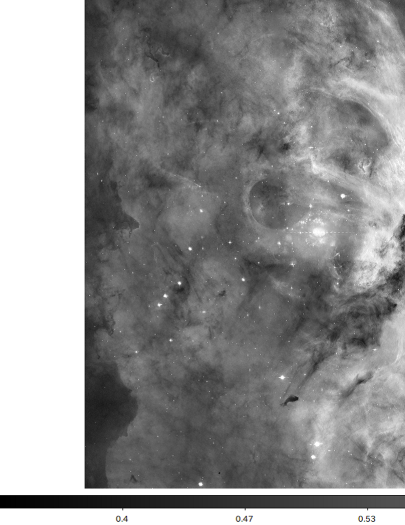
Figure 1: Test FITS image to evaluate parallelization efficiencies: a false color mosaic image of Carina Nebula obtained with Hubble Space Telescope, consisting of 29,566$\times$14,321 pixels (3.4 GB).

Table 1 shows the hardware and software configuration used for verification of the method. I used two types of CPUs, Intel Core i7-2600 (for Machine A) and AMD FX-8350 (for Machine B), to prevent bias due to microarchitecture. Through the paper, Intel Turbo Boost Technology (the former) and AMD Turbo CORE Technology (the latter) are disabled by BIOS for simplicity. In addition, Intel Hyper-Threading Technology (the former) is also disabled for the same reason. Thus Machine A and B are available 4 and 8 physical processors, respectively. The memory bandwidths and storage speeds were obtained the following commands: dd if=/dev/zero of=/dev/null bs=1G count=100, and hdparm -t (device), respectively.

The same software is installed in both computers: Ubuntu 12.04.1 LTS (amd64), a Debian based 64-bit Linux, for operating system, GNU Compiler Collection (GCC) Version 4.6 for C/C++ compiler (gcc/g++), and CFITSIO Version 3.310 for C language FITS library (Pence, 2010). I applied the -O2 -pipe -Wall compile options to CFITSIO and programs used in the paper. The Streaming SIMD Extensions 2 (SSE2) codes in CFITSIO was enabled since I built the library on a 64-bit Linux, but the SSSE3 option was disabled since the SSSE3 instruction set is treated as an extension in the amd64 environment.

I use a false color mosaic image of Carina Nebula obtained with Hubble Space Telescope for test data. The image is public in Tagged Image File Format (TIFF), thus I converted it into a gray scale double precision FITS file with convert command provided by ImageMagick. The size is 29,566 pixels in width and 14,321 pixels in height. The file volume is 3.4 GB (Figure 1). Through the paper, I put this FITS file on a tmpfs (Rohland, 2001) mounted on /run/shm, to ensure that the file is always on memory for fast access. See Appendix A for the difference between tmpfs and ramdisk.

3 Endian Conversion Algorithms

Figure 2: The schematic diagram of a permutation operator $\sigma$ for the endian conversion of a 64-bit value.

3.1 Formalism

Let $\left(b_{1},b_{2},\cdots,b_{8}\right)$ be a byte sequence of an internal expression of a 64-bit size value $a$. The 64-bit endian conversion of $a$ can be expressed with a permutation $\sigma$ as

$$a^{\prime}=\left(b_{\sigma\left(1\right)},b_{\sigma\left(2\right)},\cdots,b_{\sigma\left(8\right)}\right),$$ (1)

where

$$\sigma=\left(\begin{array}[]{cccccccc}1&2&3&4&5&6&7&8\\ 8&7&6&5&4&3&2&1\end{array}\right)$$ (2)

in Cauchy’s two-line notation, and $\sigma^{2}={\bf 1}$ (Figure 2).

3.2 Implementation

3.2.1 Byte Shuffle: Straightforward Implementation

A straightforward implementation of Eq. (1) and Eq. (2) can be written as follows:

uint64_t byte_shuffle(uint64_t a)
{
  unsigned char *p = (unsigned char *)&a;
  unsigned char tmp;

  tmp = p[7]; p[7] = p[0]; p[0] = tmp;
  tmp = p[6]; p[6] = p[1]; p[1] = tmp;
  tmp = p[5]; p[5] = p[2]; p[2] = tmp;
  tmp = p[4]; p[4] = p[3]; p[3] = tmp;

  return a;
}

I now call this method “byte shuffle”. One will find a short discussion about another implementation of byte shuffle algorithm in Appendix B.

3.2.2 Bit Shift

Another implementation to perform endian conversion is to use both bit shift and logical operations:

uint64_t bit_shift(uint64_t a)
{
  return   ((a & 0x00000000000000FFULL)
             << 56)
         | ((a & 0x000000000000FF00ULL)
             << 40)
         | ((a & 0x0000000000FF0000ULL)
             << 24)
         | ((a & 0x00000000FF000000ULL)
             << 8)
         | ((a & 0x000000FF00000000ULL)
             >> 8)
         | ((a & 0x0000FF0000000000ULL)
             >> 24)
         | ((a & 0x00FF000000000000ULL)
             >> 40)
         | ((a & 0xFF00000000000000ULL)
             >> 56);
}

Hereafter, I call this method “bit shift”.

3.2.3 BSWAP

Intel i486 and later processors have the BSWAP instruction, which converts the endian on a given 32-bit register. The instruction is extended in order to accept a 64-bit register in amd64 (Intel, 2012). Furthermore, GCC Version 4.3 and later have a helper function to call the instruction, and its prototype is uint64_t __builtin_bswap64(uint64_t x);. Now I call endian conversions utilizing this function “BSWAP”.

3.2.4 SSE2

SSE2 is a set of vector instructions for Intel platform, became a part of default instruction set for amd64 environment. The endian conversion codes utilizing SSE2 can process two 64-bit values at once, and be written as follows:

#include <emmintrin.h>
void sse2(uint64_t a[2])
{
  __m128i r0 = _mm_load_si128((__m128i *)a);
                // r0 <- a
  __m128i r1 = _mm_srli_epi16(r0, 8);
                // 8-bit shifts towards right
                // for four 2-byte integers
  __m128i r2 = _mm_slli_epi16(r0, 8);
                // 8-bit shifts towards left
                // for four 2-byte integers
  r0 = _mm_or_si128(r1, r2);
                // 128-bit or operation
                // on r1 and r2
  r0 = _mm_shufflelo_epi16(r0,
               _MM_SHUFFLE(0, 1, 2, 3));
                // byte shuffle for the
                // lower half of r0 register
  r0 = _mm_shufflehi_epi16(r0,
               _MM_SHUFFLE(0, 1, 2, 3));
                // byte shuffle for the
                // higher half of r0 register
  _mm_store_si128((__m128i *)a, r0);
                // a <- r0
}

There are almost the same codes in CFITSIO and SLLIB/SFITSIO. I call these codes simply “SSE2”, hereafter.

3.3 SSSE3

Another vector instruction set called “SSSE3” is available for Intel Core series and later CPUs. Utilizing this instruction set, one can perform endian conversion of two 64-bit values at one instruction. An example is follows:

#include <tmmintrin.h>
void ssse3(uint64_t a[2])
{
  static const __m128i mask
    = _mm_set_epi8(
        8, 9, 10, 11, 12, 13, 14, 15,
        0, 1, 2 ,3, 4, 5, 6, 7
      );
  __m128i r = _mm_load_si128((__m128i *)a);
  __m128i r = _mm_shuffle_epi8(r, mask);
  _mm_store_si128((__m128i *)a, r);
}

There are almost same codes in CFITSIO too. I call these codes simply “SSSE3”, hereafter.

Table 2: Endian Conversion Time

Machine	Bit Shift (msec)	BSWAP (msec)	SSE2 (msec)	SSSE3 (msec)	Byte Shuffle (msec)
Machine A	$410\pm 2$	$410\pm 2$	$405\pm 2$	$372.4\pm 0.1$	$3190.3\pm 0.6$
Machine B	$601.3\pm 0.6$	$605.8\pm 0.7$	$582.3\pm 0.7$	$598\pm 2$	$8056.3\pm 0.3$

Note. — The endian conversion time of 423,414,686 ($=$29,566$\times$14,321) double-type elements with various algorithms.

3.4 Benchmark

To see which one is fastest and how they behave towards parallelization, I performed simple benchmark. In the benchmark, I reserved a double-type array whose number of elements were set to 29,566$\times$14,321 = 423,414,686, just the number of pixels in Figure 1, and filled the array for uniform real random numbers of 32-bit resolution on $[-1000,1000]$ generated with Mersenne Twister (Matsumoto & Nishimura, 1998).

3.4.1 Single Thread

The results are summarized in Table 2. For Machine A, three algorithms except for SSSE3 and byte shuffle process the test data in about 410 milliseconds, while SSSE3 does about 370 millisecond. On the other hand, for Machine B, four algorithms except for byte shuffle process the test data in about 600 milliseconds, and the SSE2 algorithm is fastest in the all ones. The byte shuffle algorithm is slowest by one oder compared to the others.

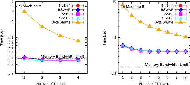
Figure 3: CPU-scalability comparison between the endian coversion algorithms. All the algorithms except for byte shuffle seem to behave in the same way and scale up to only the half number of CPU cores due to the hardware I/O limits.

Table 3: The CPU-scalability of the endian conversion alogorithms on Machine A

Number of Threads	Bit Shift (msec)	BSWAP (msec)	SSE2 (msec)	SSSE3 (msec)	Byte Shuffle (msec)
1	$410\pm 2$	$411\pm 3$	$404\pm 2$	$372.4\pm 0.2$	$3191.8\pm 0.7$
2	$366\pm 3$	$366\pm 3$	$367\pm 2$	$360.4\pm 0.5$	$1605\pm 2$
3	$362\pm 3$	$362\pm 3$	$362\pm 3$	$354.9\pm 0.3$	$1082\pm 6$
4	$365\pm 4$	$365\pm 4$	$365\pm 4$	$358.8\pm 0.5$	$860\pm 20$

Note. — The CPU-scalability of 423,414,686 ($=$29,566$\times$14,321) double-type element endian conversion with various algorithms on Machine A. Different from Table 2, 16-byte memory alignment is adopted.

Table 4: The CPU-scalability of the endian conversion alogorithms on Machine B

Number of Threads	Bit Shift (msec)	BSWAP (msec)	SSE2 (msec)	SSSE3 (msec)	Byte Shuffle (msec)
1	$597.8\pm 0.7$	$605.1\pm 0.7$	$579.3\pm 0.9$	$597\pm 2$	$8056.2\pm 0.2$
2	$484\pm 1$	$499\pm 1$	$484\pm 1$	$495\pm 1$	$4046\pm 3$
3	$429.9\pm 0.8$	$445\pm 3$	$432\pm 1$	$440\pm 1$	$2699\pm 4$
4	$413\pm 3$	$412\pm 2$	$413\pm 3$	$419\pm 7$	$2031\pm 8$
5	$418\pm 3$	$417\pm 1$	$422\pm 2$	$424\pm 2$	$1661\pm 5$
6	$412\pm 1$	$411.5\pm 0.8$	$413\pm 1$	$416\pm 1$	$1388\pm 4$
7	$412.3\pm 0.9$	$412.2\pm 0.5$	$411.9\pm 0.6$	$414.1\pm 0.5$	$1192\pm 4$
8	$416.1\pm 0.6$	$415.1\pm 0.7$	$415.5\pm 0.4$	$414.5\pm 0.4$	$1043\pm 2$

Note. — All conditions are same as Table 3.

3.4.2 Multi-Thread

I also examined the CPU-scalability of these algorithms. I adopted pthread for parallelization, and simply divided the array containing the test data into equal-size segments so that the total number of the segments were equal to the number of threads. Then I assigned each thread with each segment.

Figure 3 represents the results. I also list the observed values for detailed comparison of the algorithms in Table 3 (for Machine A) and Table 4 (for Machine B). Except for byte shuffle algorithm, I observed $\simeq 10\%$ performance gain for Machine A, and $\simeq 40\%$ up to four threads for Machine B with the four algorithms.

It seems strange that the memory bandwidth of Machine B is sufficient for the test data size but the four algorithms show performance cutoff at four threads. I performed detailed hardware benchmark utilizing LMbench, and found that context switching time and the latency of L2 cache memory normalized in CPU cycles of Machine B are 2.4 times and 4.6 times, respectively, larger than those of Machine A. Hence I conclude that there are some hardware bottlenecks in Machine B, which cause the plateau in Figure 3.

The behaviors of the four algorithms with respect to the number of threads are very similar, and I adopt bit shift algorithm in the next section because of its compiler portability and identicalness to BSWAP (see Appendix C).

4 Endian Conversion Timing

A modern CPU has multiple arithmetic logic units (ALUs) and instruction pipelines to boost the operating rates of ALUs. As seen in the previous section, the hardware limitation lies just below the endian conversion time of single thread (Figure 3, Machine A), preventing the CPU scalability. This may lead to many holes (or “no operation” instructions) in the pipelines and reduce the performance. If this is the case, shuffling instructions in source codes can produce improvement.

To verify this assumption, I disabled the endian conversion functionality in CFITSIO; I changed the BYTESWAPPED macros for i386 and amd64 architectures from TRUE into FALSE in fitsio2.h, and commented out the codes which CFITSIO perform runtime check to verify whether the machine endian definition by the above macro is consistent with the execution environment in cfileio.c, and I rebuilt the library. The patches for those files are shown in Appendix E.

I compare the following two methods;

1. It loads the full test image (Figure 1) from tmpfs (see §2) onto an array, then it converts the endian by the parallelized bit shift algorithm (described in §3.4.2), and it sums up all the elements.

2. It loads the full test image onto an array, and it sums up all the elements with converting the endian one after another by the bit shift algorithm.

From here, I refer to the former as “on ahead endian conversion method”, and to the latter as “just-in-time endian conversion method”.

On ahead endian conversion method can be written as follows:

{
  double *v;   // an array to store
               // a FITS image
  size_t len;  // the length of
               // the array v

  // load a byte sequence from a FITS
  // file into v here...

  // endian conversion
  for (size_t i = 0; i < len; ++i) {
    uint64_t *p = (uint64_t *)&v[i];
    uint64_t a = bit_shift(*p);
    double *q = (double *)&a;
    v[i] = *q;
  }

  // process v here...
}

and just-in-time endian conversion method can be written as follows:

{
  double *v;   // an array to store
               // a FITS image
  size_t len;  // the length of
               // the array v

  // load a byte sequence from a FITS
  // file into v here...

  // image processing...
  {
    // something...

    // one needs to refer the value
    // of v[i] here

    // endian conversion
    uint64_t *p = (uint64_t *)&v[i];
    uint64_t a = bit_shift(*p);
    double *q = (double *)&a;
    double x = *q;
    // use x instead of v[i] below

    // something...
  }
}

where bit_shift() is the endian conversion function defined in §3.2.2.

In this section, I adopt summing up all the elements in the test image as an example of image processing.

4.1 Single Thread

I implemented both methods in single thread and performed benchmark. The codes of on ahead conversion method are following:

{
  // endian conversion
  for (size_t i = 0; i < len; ++i) {
    uint64_t *p = (uint64_t *)&v[i];
    uint64_t a = bit_shift(*p);
    double *q = (double *)&a;
    v[i] = *q;
  }

  // summation
  double sum = 0.0;
  for (size_t i = 0; i < len; ++i) {
    sum += v[i];
  }
}

and those of just-in-time endian conversion method are following:

{
  double sum = 0.0;
  for (size_t i = 0; i < len; ++i) {
    // endian conversion
    uint64_t *p = (uint64_t *)&v[i];
    uint64_t a = bit_shift(*p);
    double *q = (double *)&a;

    // summation
    sum += *q;
  }
}

Note that the former codes are identical to those with original CFITSIO.

The results are summarized in Table 5. I obtained slightly faster ($\simeq 5\%$) total processing time of $2.22\pm 0.04$ sec and $3.62\pm 0.04$ sec for Machine A and B, respectively, with on ahead endian conversion method, while that with original CFITSIO is $2.38\pm 0.04$ and $3.79\pm 0.03$ for Machine A and B, respectively.

On the other hand, I obtained significantly faster time of $1.85\pm 0.04$ and $3.05\pm 0.03$ for Machine A and B, respectively, which corresponds to $\simeq 25\%$ performance gain, with just-in-time endian conversion method.

4.2 Multi-Thread

I made both methods multithreaded by utilizing OpenMP APIs for its simple implementation. The codes of just-in-time endian conversion method, for example, are below:

{
  double sum = 0.0;
  #pragma omp parallel for reduction (+:sum)\\
schedule (auto)
  for (size_t i = 0; i < len; ++i) {
    // endian conversion
    uint64_t *p = (uint64_t *)&v[i];
    uint64_t a = bit_shift(*p);
    double *q = (double *)&a;

    // summation
    sum += *q;
  }
}

On the other hand, I could not find the best parameters in OpenMP APIs for the endian conversion routine in on ahead conversion method, hence I applied OpenMP only to the summation routine, and adopted the pthread-based parallelization described in §3.4.2 for the endian conversion routine in on ahead conversion method; the number of the threads for OpenMP was set to that for the endian conversion.

The results obtained with these programs are summarized in Table 6 (for Machine A), Table 7 (for Machine B), Figure 4 (for on ahead endian conversion method), and Figure 5 (for just-in-time endian conversion method). Note that the endian conversion time of on ahead endian conversion method is included in the FITS reading time. The total time to perform the same things with the original CFITSIO in single thread is superimposed on these figures as a dotted line: $2.38\pm 0.04$ seconds for Machine A, and $3.79\pm 0.03$ seconds for Machine B.

For the on ahead endian conversion method, the total time slightly scales the number of threads and gets faster than original CFITSIO, while the file reading time (including endian conversion time) seems to be little scalable. The scalability of the total time mostly owes that of the summation routine, and the parallelization of the endian conversion has little impact due to the hardware limit seen in §3.4.2.

On the other hand, for the just-in-time endian conversion method, the total time is interestingly smaller than that of original CFITSIO even for single thread. The summation routine seems to be scalable almost in the full range, while the total time scales up to four threads.

Table 5: The data processing times with two different method in single thread

Method	Machine	FITS Read Time (sec)	Sum Up Time (sec)	Total Time (sec)
	Machine A	$1.006\pm 0.003$	$0.4198\pm 0.0002$	$2.22\pm 0.04$
On Ahead Endian Conversion	Machine B	$1.859\pm 0.007$	$0.557\pm 0.001$	$3.62\pm 0.04$
	Machine A	$1.010\pm 0.003$	$0.44003\pm 0.00008$	$1.85\pm 0.04$
Lasy Endian Conversion	Machine B	$1.874\pm 0.007$	$0.621\pm 0.002$	$3.06\pm 0.03$

Note. — The total time with original CFITSIO is $2.38\pm 0.04$ and $3.79\pm 0.03$ for Machine A and B, respectively.

Table 6: The CPU-scalability of on ahead and just-in-time endian conversion methods on Machine A

Method	Number of Threads	FITS Read Time (sec)	Sum Up Time (sec)	Total Time (sec)
	1	$1.445\pm 0.003$	$0.4205\pm 0.0001$	$2.38\pm 0.04$
	2	$1.404\pm 0.003$	$0.220\pm 0.004$	$2.1\pm 0.1$
On Ahead Endian Conversion Method	3	$1.401\pm 0.003$	$0.181\pm 0.002$	$2.11\pm 0.09$
	4	$1.403\pm 0.003$	$0.177\pm 0.002$	$2.09\pm 0.03$
	1	$1.048\pm 0.003$	$0.4416\pm 0.0009$	$2.0\pm 0.1$
	2	$1.051\pm 0.003$	$0.2262\pm 0.0005$	$1.8\pm 0.1$
Just-in-Time Endian Conversion Method	3	$1.051\pm 0.003$	$0.183\pm 0.001$	$1.77\pm 0.02$
	4	$1.052\pm 0.003$	$0.177\pm 0.002$	$1.76\pm 0.02$

Note. — The endian conversion time is included in the FITS reading time for on ahead endian conversion method.

Table 7: The CPU-scalability of on ahead and just-in-time endian conversion methods on Machine B

Method	Number of Threads	FITS Read Time (sec)	Sum Up Time (sec)	Total Time (sec)
	1	$2.526\pm 0.005$	$0.5522\pm 0.0006$	$3.76\pm 0.03$
	2	$2.403\pm 0.005$	$0.299\pm 0.003$	$3.39\pm 0.01$
	3	$2.347\pm 0.005$	$0.220\pm 0.002$	$3.253\pm 0.010$
	4	$2.326\pm 0.005$	$0.193\pm 0.003$	$3.203\pm 0.008$
On Ahead Endian Conversion Method	5	$2.334\pm 0.006$	$0.205\pm 0.003$	$3.224\pm 0.010$
	6	$2.326\pm 0.005$	$0.189\pm 0.003$	$3.20\pm 0.01$
	7	$2.325\pm 0.006$	$0.178\pm 0.002$	$3.19\pm 0.01$
	8	$2.334\pm 0.005$	$0.174\pm 0.003$	$3.19\pm 0.01$
	1	$1.914\pm 0.003$	$0.582\pm 0.002$	$3.19\pm 0.05$
	2	$1.917\pm 0.003$	$0.328\pm 0.002$	$2.934\pm 0.009$
	3	$1.916\pm 0.004$	$0.242\pm 0.002$	$2.853\pm 0.008$
	4	$1.916\pm 0.004$	$0.205\pm 0.002$	$2.812\pm 0.009$
Just-in-Time Endian Conversion Method	5	$1.918\pm 0.003$	$0.205\pm 0.001$	$2.816\pm 0.009$
	6	$1.918\pm 0.003$	$0.1948\pm 0.0009$	$2.801\pm 0.010$
	7	$1.917\pm 0.004$	$0.185\pm 0.001$	$2.791\pm 0.010$
	8	$1.917\pm 0.003$	$0.178\pm 0.003$	$2.781\pm 0.010$

Note. — The endian conversion time is included in the FITS reading time for on ahead endian conversion method.

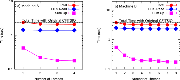
Figure 4: The CPU-scalability of the FITS reading and processing time by applying the bit shift parallel algorithm to CFITSIO. I also applied a simple OpenMP parallelization to the summation routine.

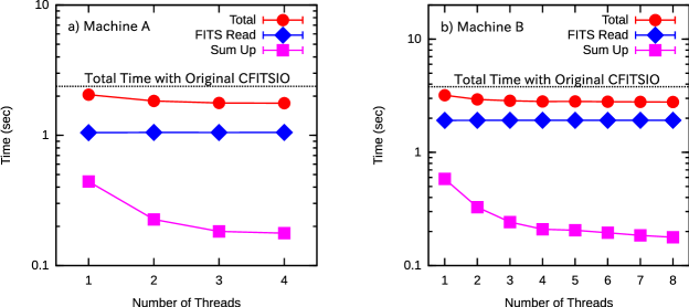
Figure 5: The CPU-scalability of the just-in-time endian conversion algorithm. Endian conversions are performed in the summation routine, which is applied a simple OpenMP parallelization.

5 Discussion

5.1 Performance Analysis of the Simple Summation Codes

There is a well-known equation to estimate the increase by parallelization, Amdahl’s law (Amdahl, 1967):

$$T_{\rm parallel}=\left\{\left(1-P\right)+\frac{P}{N}+\alpha\right\}T_{\rm single},$$ (3)

where $T_{\rm single}$ and $T_{\rm parallel}$ represent processing time in single thread and mult-thread cases, respectively, $P$ is the ratio of codes which parallelization methods are applied to, $N$ is the number of threads, and $\alpha$ is the overhead caused by parallelization.

To quantify the performance increase of on ahead endian conversion method and just-in-time endian conversion method, I performed model fitting to the total time of both methods with Eq.(3). I found that $\alpha\sim O\left(10^{-30}\right)$ while the fitting, thus I fixed $\alpha$ at 0. The results are summarized in Table 8 and Figure 6. The increasing rates of performance compared to original CFITSIO ($T_{\rm single}=2.38\pm 0.04$ for Machine A and $T_{\rm single}=3.79\pm 0.03$ for Machine B) are also listed in the table.

The figure shows that the above results are explained well by Amdahl’s law, and that the on ahead endian conversion method for single thread has almost the same performance as original CFITSIO. In fact, these two agree with each other in $\lesssim 5\%$ errors according to the table. The table also suggests that multi-threading boosts this method up about 20%. Considering the parallelization rate $P\simeq 16\%$, one cannot expect further speed up by multi-threading in $N\gtrsim 4$. This suggests that the bottlenecks of other hardwares disrupt order in the instruction pipelines and leads to the decrease of operating ratio of ALUs.

On the other hand, the just-in-time endian conversion method is 20% faster than both of original CFITSIO and the single thread version of on ahead one, surprisingly. This seems as if the endian conversion process disappeared. In the parallelized case, the just-in-time conversion method is 40% faster than the others in single thread. However, the performance increase by multi-threading can be expected only in $N\lesssim 4$ since the parallelization rate $P\simeq 16\%$, due to the hardware bottlenecks mentioned above.

For further investigation, I fitted the summation time of these methods with Eq.(3) to investigate the impact of the endian conversion codes in the summation routine on performance; there are endian conversion codes in the summation routine in case of just-in-time endian conversion method, but not in case of on ahead endian conversion method. The results are summarized in Table 9 and Figure 7. I found that the parallelization rate $P\approx 85\%$ in both cases, and that the ratio of $T_{\rm single}$ of just-in-time endian conversion method against that of on ahead one $r=T_{\rm single}\left({\rm Just-in-Time}\right)/T_{\rm single}\left({\rm On\ Ahead}\right)$ was equal to $r=1.02\pm 0.05$ for Machine A and $r=1.03\pm 0.04$ for Machine B. There is no overhead of endian conversion in the summation routine, since the shift of $r$ from unity is not significant statistically.

Thus I conclude that endian conversion is so simple operation for a modern CPU that the bottlenecks of other hardwares disrupt order in the instruction pipelines; to prevent the disruption, the endian conversion should be done just before a value is referred.

Table 8: The fitting results of the total processing time

					Increase Rate of Performance
Method	Machine	$T_{\rm single}$ (sec)	$P$	$\chi^{2}$ (d.o.f.a)	Single Thread	Multi-Thread
	Machine A	$2.377\pm 0.009$	$0.164\pm 0.006$	0.09 (2)	$1.00\pm 0.02$	$1.20\pm 0.02$
On Ahead Endian Conversion	Machine B	$3.68\pm 0.05$	$0.16\pm 0.02$	49b (6)	$1.03\pm 0.02$	$1.22\pm 0.03$
	Machine A	$2.02\pm 0.05$	$0.17\pm 0.03$	0.5 (2)	$1.18\pm 0.04$	$1.42\pm 0.07$
Just-in-Time Endian Conversion	Machine B	$3.13\pm 0.02$	$0.130\pm 0.009$	8.5 (6)	$1.21\pm 0.01$	$1.39\pm 0.02$

Note. — The fitting results of the total processing time with respect to two different endian conversion methods with Amdahl’s law and their increase rate of performance compared with original CFITSIO ($T_{\rm single}=2.38\pm 0.04$ for Machine A and $T_{\rm single}=3.79\pm 0.03$ for Machine B). The errors are 1-$\sigma$ confidence limits for a single parameter.

Table 9: The fitting results of the time to sum up all elements

Method	Machine	$T_{\rm single}$ (msec)	$P$	$\chi^{2}$ (d.o.f.)
	Machine A	$420\pm 1$	$0.82\pm 0.04$	127.9 (2)
On Ahead Endian Conversion	Machine B	$551\pm 6$	$0.81\pm 0.02$	491.1 (6)
	Machine A	$430\pm 20$	$0.92\pm 0.06$	913.4 (2)
Just-in-Time Endian Conversion	Machine B	$570\pm 20$	$0.80\pm 0.02$	312.7 (6)

Note. — $T_{\rm single}\left({\rm Just-in-Time}\right)/T_{\rm single}\left({\rm On\ Ahead}\right)=1.02\pm 0.05$ (for Machine A), $1.03\pm 0.04$ (for Machine B).

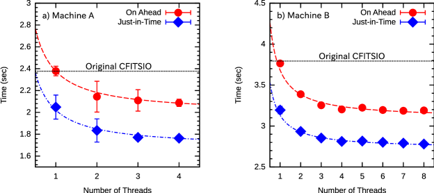
Figure 6: The fitting results of on ahead and just-in-time endian conversion method with respect to total processing time with Amdahl’s law. The red dashed and blue dash dotted lines correspond to the law for on ahead and just-in-time endian conversion method, respectively.

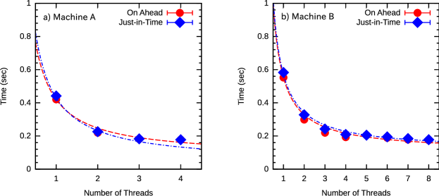
Figure 7: The fitting results of on ahead and just-in-time endian conversion method with respect to summation time with Amdahl’s law. The red dashed and blue dash dotted lines correspond to the law for on ahead and just-in-time endian conversion method, respectively.

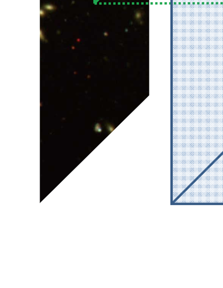
Figure 8: The schematic illustration of a data cube of ALMA Science Verification Data.

Table 10: Image Extraction Time

File Size (MB)	On Ahead Endian Conversion Method	Just-in-Time Endian Conversion Method
$21.4$	$0.02953\pm 0.00006$	$0.0361\pm 0.0004$
$55.0$	$0.75214\pm 0.00003$	$0.0910\pm 0.0001$
$66.9$	$0.10007\pm 0.00006$	$0.10295\pm 0.00008$
$78.4$	$0.13136\pm 0.00008$	$0.12371\pm 0.00008$
$88.7$	$0.14435\pm 0.00007$	$0.1299\pm 0.0001$
$106.9$	$0.1835\pm 0.0001$	$0.1606\pm 0.0002$
$150.3$	$0.2333\pm 0.0001$	$0.21006\pm 0.00008$

Note. — The time to extract an image from an ALMA data cube on Machine A in single thread.

Table 11: Spectrum Extraction Time

File Size (MB)	On Ahead Endian Conversion Method	Just-in-Time Endian Conversion Method
$21.4$	$0.02743\pm 0.00002$	$0.0344\pm 0.0004$
$55.0$	$0.06970\pm 0.00002$	$0.07527\pm 0.00008$
$66.9$	$0.08512\pm 0.00002$	$0.08583\pm 0.00010$
$78.4$	$0.09861\pm 0.00003$	$0.0909\pm 0.0001$
$88.7$	$0.11271\pm 0.00003$	$0.10539\pm 0.00008$
$106.9$	$0.13394\pm 0.00004$	$0.1153\pm 0.0003$
$150.3$	$0.18769\pm 0.00005$	$0.15503\pm 0.00006$

Note. — The time to extract a spectrum from an ALMA data cube on Machine A in single thread.

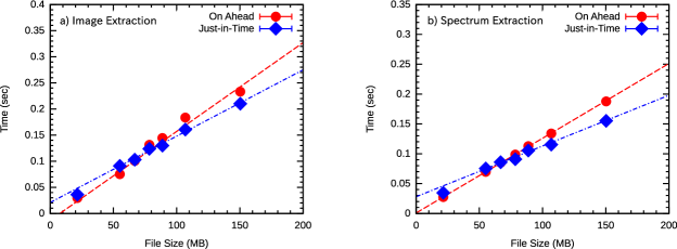
Figure 9: The image (left) and spectrum (right) extraction time with respect to file size of ALMA data cube. The red dashed and blue dash dotted lines correspond to the best fit ones for on ahead and just-in-time endian conversion method, respectively.

5.2 Application to ALMAWebQL

From here, I only investigated the performance increase of summing up all the elements in a large FITS file by just-in-time endian conversion method. In this subsection, I apply the method to ALMAWebQL, our interactive web viewer for ALMA data cubes described in Paper I, to obtain more realistic benchmark data. For realistic and fair comparison, the SSE2 boosted endian conversion codes in CFITSIO are enabled for on ahead endian conversion method, while there is no SSE2 code in just-in-time endian conversion method.

ALMA data cubes not contain information of polarization currently, and they are simple 3-dimensional FITS files (Figure 8). For image extraction, one have to integrate the cube along the spectral direction; for spectrum extraction, one convolute all spatial information.

I measured the time to complete these computations in single thread with various size data on Machine A. The results for image extraction are summarized in Table 10, and those for spectrum extraction are summarized in Table 11. From these tables, I obtain

$$T\left({\rm On\ Ahead}\right) = \left(1.7\pm 0.1\right)\times 10^{-3}\left(\frac{V}{\rm MB}\right)$$ (4)

$$-\left(0.013\pm 0.007\right)\ \sec,$$

$$T\left({\rm Just-in-Time}\right) = \left(1.27\pm 0.04\right)\times 10^{-3}\left(\frac{V}{\rm MB}\right)$$ (5)

$$+\left(0.021\pm 0.003\right)\ \sec$$

for image extraction and

$$T\left({\rm On\ Ahead}\right) = \left(1.252\pm 0.007\right)\times 10^{-3}\left(\frac{V}{\rm MB}\right)$$ (6)

$$+\left(0.0008\pm 0.0004\right)\ \sec,$$

$$T\left({\rm Just-in-Time}\right) = \left(0.85\pm 0.02\right)\times 10^{-3}\left(\frac{V}{\rm MB}\right)$$ (7)

$$+\left(0.028\pm 0.002\right)\ \sec$$

for spectrum extraction, where $T\left({\rm On\ Ahead}\right)$ and $T\left({\rm Just-in-Time}\right)$ represent the time with on ahead and just-in-time endian conversion methods, respectively, and $V$ is file size in the MB unit (Figure 9). Hence just-in-time endian conversion method in single thread is $\gtrsim 20\%$ faster than on ahead conversion method boosted by SSE2 above $V\gtrsim 200\ \rm{MB}$. This demonstrates that just-in-time endian conversion method can be very powerful when one performs convolution and stacking of very large images, which are very common analysis techniques in optical band, obtained with future large telescopes.

5.3 Data Types

In this paper, I only treated a double precision FITS file, but one could expect almost the same results for float and LONG data types, which correspond to BITPIX $=$ -32 and 32, respectively; as demonstrated in Appendix C, bit_shift() function is compiled into BSWAP instruction. The amd64 architecture can handle both of 32 bit and 64 bit operation codes and their operands seamlessly. On the other hand, for byte and short data type, there may be little advantage of just-in-time endian conversion method since BSWAP instruction cannot take any 16 bit values as its operand, and up-casting into 32 bit integer always occurs in arithmetic operations in both cases.

6 Summary

The FITS format was originally developed to exchange digital astronomical datasets from a computer to another, but the progress of computation power and software technology enables one to process FITS files through web browsers. In addition, data size has been inflating year by year, and it will exceed $\sim$ TB in the year ahead. To handle such big FITS file with web applications, the endian conversion time from the FITS native to the machine one cannot be negligible, and a solution for this problem is required.

In this paper, I compared the features of four typical endian conversion algorithms under multi-thread environment, and found the bit shift one was suitable for parallelization. Then I examined the best timing for endian conversion under multi-thread environment. I found that one should postpone the endian conversion until a value is really referred in a program, because endian conversion is so simple for a modern CPU that the bottlenecks of other hardwares disrupt order in the instruction pipelines, which leads to the decrease of operating ratio of ALUs. In fact, by applying this method to loading 3.4 GB FITS file and sum up all the elements, the performance increased 20% for single thread and 40% for multi-thread compared to CFITSIO, which corresponded to $\gtrsim 600$ milliseconds, and one can be aware of the speed-up. No overhead of endian conversion was found on the summation routine; hence one can sweep the endian conversion time out of his/her codes. Note that parallelization of this method peaked out in four threads in the experiment.

CPU vendors introduce various techniques, such as speculative execution and branch prediction, to improve the efficiency of instruction pipelines; an executed instruction code sequence is apart from a programmed one. In this context, modern CPUs partially break “causality”, a programmed instruction code sequence, and gain speed. Just-in-time endian conversion method utilizes such boosting technology. There is nothing new in the method, but it must be a small step to handle astronomical big data generated by the next generation telescopes.

Appendix A Tmpfs and Ramdisk

Both tmpfs and ramdisk are a data space allocated on memory. One has to specify the size in advance for ramdisk, while one does not set the size for tmpfs in advance necessarily since it is under control of virtual memory manager and shares swap space.

When an application requests the operating system for memory blocks and when there does not remain sufficient physical memory space, the memory manager firstly swap out the files on tmpfs. Tmpfs is ideal space to put temporal files which one requires very fast access to.

Appendix B Another Implementation of Byte Shuffle Algorithm

One can also implements byte shuffle algorithm as follows:

uint64_t byte_shuffle2(uint64_t a)
{
  unsigned char *p = (unsigned char *)&a;
  uint64_t b;
  unsigned char *q = (unsigned char *)&b;

  q[0] = p[7];
  q[1] = p[6];
  q[2] = p[5];
  q[3] = p[4];
  q[4] = p[3];
  q[5] = p[2];
  q[6] = p[1];
  q[7] = p[0];

  return b;
}

The number of assignments of the codes ($=8$) is less than that shown in the main part of this paper ($=12$), and one would expect further performance improvement.

I disassembled both two codes compiled with the -O2 option, and obtained followings:

0000000000000000 <byte_shuffle>:
   0:Ψ49 89 fa             Ψmov    %rdi,%r10
   3:Ψ49 89 f8             Ψmov    %rdi,%r8
   6:Ψ89 fe                Ψmov    %edi,%esi
   8:Ψ48 89 f9             Ψmov    %rdi,%rcx
   b:Ψ89 fa                Ψmov    %edi,%edx
   d:Ψ48 89 f8             Ψmov    %rdi,%rax
  10:Ψ40 88 7c 24 ff       Ψmov    %dil,-0x1(%rsp)
  15:Ψ48 c1 e8 20          Ψshr    $0x20,%rax
  19:Ψ49 c1 ea 38          Ψshr    $0x38,%r10
  1d:Ψ49 c1 e8 30          Ψshr    $0x30,%r8
  21:Ψ66 c1 ee 08          Ψshr    $0x8,%si
  25:Ψ48 c1 e9 28          Ψshr    $0x28,%rcx
  29:Ψc1 ea 10             Ψshr    $0x10,%edx
  2c:Ψc1 ef 18             Ψshr    $0x18,%edi
  2f:Ψ44 88 54 24 f8       Ψmov    %r10b,-0x8(%rsp)
  34:Ψ40 88 74 24 fe       Ψmov    %sil,-0x2(%rsp)
  39:Ψ44 88 44 24 f9       Ψmov    %r8b,-0x7(%rsp)
  3e:Ψ88 54 24 fd          Ψmov    %dl,-0x3(%rsp)
  42:Ψ88 4c 24 fa          Ψmov    %cl,-0x6(%rsp)
  46:Ψ40 88 7c 24 fc       Ψmov    %dil,-0x4(%rsp)
  4b:Ψ88 44 24 fb          Ψmov    %al,-0x5(%rsp)
  4f:Ψ48 8b 44 24 f8       Ψmov    -0x8(%rsp),%rax
  54:Ψc3                   Ψretq

, and

0000000000000000 <byte_shuffle2>:
   0:Ψ49 89 fa             Ψmov    %rdi,%r10
   3:Ψ49 89 f9             Ψmov    %rdi,%r9
   6:Ψ49 89 f8             Ψmov    %rdi,%r8
   9:Ψ48 89 fe             Ψmov    %rdi,%rsi
   c:Ψ89 f9                Ψmov    %edi,%ecx
   e:Ψ89 fa                Ψmov    %edi,%edx
  10:Ψ89 f8                Ψmov    %edi,%eax
  12:Ψ49 c1 ea 38          Ψshr    $0x38,%r10
  16:Ψ49 c1 e9 30          Ψshr    $0x30,%r9
  1a:Ψ66 c1 e8 08          Ψshr    $0x8,%ax
  1e:Ψ49 c1 e8 28          Ψshr    $0x28,%r8
  22:Ψ48 c1 ee 20          Ψshr    $0x20,%rsi
  26:Ψc1 e9 18             Ψshr    $0x18,%ecx
  29:Ψc1 ea 10             Ψshr    $0x10,%edx
  2c:Ψ44 88 54 24 f8       Ψmov    %r10b,-0x8(%rsp)
  31:Ψ44 88 4c 24 f9       Ψmov    %r9b,-0x7(%rsp)
  36:Ψ44 88 44 24 fa       Ψmov    %r8b,-0x6(%rsp)
  3b:Ψ40 88 74 24 fb       Ψmov    %sil,-0x5(%rsp)
  40:Ψ88 4c 24 fc          Ψmov    %cl,-0x4(%rsp)
  44:Ψ88 54 24 fd          Ψmov    %dl,-0x3(%rsp)
  48:Ψ88 44 24 fe          Ψmov    %al,-0x2(%rsp)
  4c:Ψ40 88 7c 24 ff       Ψmov    %dil,-0x1(%rsp)
  51:Ψ48 8b 44 24 f8       Ψmov    -0x8(%rsp),%rax
  56:Ψc3                   Ψretq

, that is, there are less assignments in byte_shuffle2() ($=8$) than byte_shuffle() ($=12$), however, the former binary codes are longer than the latter ones. Hence one cannot expect more performance gain with the codes.

Appendix C Bit Shift Algorithm and BSWAP Instruction

The bit shift endian conversion codes is actually identical to BSWAP instruction when compiled with the optimization option of -O2. The disassembled codes obtained with objdump -d command are below:

0000000000000000 <bit_shift>:
   0:   48 89 f8                mov    %rdi,%rax
   3:   48 0f c8                bswap  %rax
   6:   c3                      retq

Table 12: The endian conversion time in case that memory alignment is random

Machine	Bit Shift (msec)	BSWAP (msec)	SSE2 (msec)	SSSE3 (msec)	Byte Shuffle (msec)
Machine A	$413\pm 2$	$416\pm 3$	$416\pm 5$	$377\pm 2$	$3220\pm 10$
Machine B	$624\pm 7$	$641\pm 9$	$602\pm 9$	$590\pm 3$	$8320\pm 90$

Note. — The endian conversion time of 423,414,686 ($=$29,566$\times$14,321) double-type elements with various algorithms in case that memory alignment is random.

Appendix D Endian Conversion Algorithms and Memory Alignment

It is ensured that the leading memory address (alignment) of an array is always in multiplies of 16 (16-byte alignment) in amd64 architecture. However, if one would like to read a file in multi-thread, he/she has to make the copy of the file image on memory. In such case, the alignment is not always 16-byte. Thus I performed the benchmark described in §3.4 (single thread case) but made alignment of the arraya random number.

For the benchmark, I modified _mm_load_si128() and _mm_store_si128() in the SSE2 codes into _mm_loadu_si128() and _mm_storeu_si128(), respectively, to make the codes operable. The results are summarized in Table 12.

The trend found in §3.4.1 is roughly true in this case though the all algorithms are slightly slower (within a few %) than 16-byte alignment case. Hence one does not have to get nervous about memory alignment.

Appendix E The Patches for CFITSIO

E.1 fitsio2.h

*** fitsio2.h.orgΨ2013-03-08 14:19:49.560538980 +0900
--- fitsio2.hΨ2013-01-15 14:43:10.000000000 +0900
***************
*** 96,102 ****

  #elif defined(__ia64__)  || defined(__x86_64__)
                    /*  Intel itanium 64-bit PC, or AMD opteron 64-bit PC */
! #define BYTESWAPPED TRUE
  #define LONGSIZE 64

  #elif defined(_SX)             /* Nec SuperUx */
--- 96,103 ----

  #elif defined(__ia64__)  || defined(__x86_64__)
                    /*  Intel itanium 64-bit PC, or AMD opteron 64-bit PC */
! /* #define BYTESWAPPED TRUE */
! #define BYTESWAPPED FALSE
  #define LONGSIZE 64

  #elif defined(_SX)             /* Nec SuperUx */
***************
*** 169,175 ****

  /*  generic 32-bit IBM PC */
  #define MACHINE IBMPC
! #define BYTESWAPPED TRUE

  #elif defined(__arm__)

--- 170,178 ----

  /*  generic 32-bit IBM PC */
  #define MACHINE IBMPC
! /* #define BYTESWAPPED TRUE */
! #define BYTESWAPPED FALSE
!

  #elif defined(__arm__)

E.2 cfileio.c

*** cfileio.c.orgΨ2013-03-08 14:20:09.052539296 +0900
--- cfileio.cΨ2013-01-16 19:57:46.000000000 +0900
***************
*** 3763,3769 ****
      }

      /*   test for correct byteswapping.   */
!
      u.ival = 1;
      if  ((BYTESWAPPED && u.cval[0] != 1) ||
           (BYTESWAPPED == FALSE && u.cval[1] != 1) )
--- 3763,3769 ----
      }

      /*   test for correct byteswapping.   */
! /*
      u.ival = 1;
      if  ((BYTESWAPPED && u.cval[0] != 1) ||
           (BYTESWAPPED == FALSE && u.cval[1] != 1) )
***************
*** 3776,3782 ****
        FFUNLOCK;
        return(1);
      }
!

      /*  test that LONGLONG is an 8 byte integer */

--- 3776,3782 ----
        FFUNLOCK;
        return(1);
      }
! */

      /*  test that LONGLONG is an 8 byte integer */

References

- Amdahl (1967) Amdahl, G. M., Proceedings of the April 18-20, 1967, Spring Joint Computer Conference, AFIPS ’67 (Spring), 483
- Eguchi et al. (2012) Eguchi, S., Kawasaki, W., Shirasaki, Y., et al. 2012, arXiv:1211.3790
- Greisen & Harten (1981) Greisen, E. W., & Harten, R. H. 1981, A&AS, 44, 371
- Grosbol et al. (1988) Grosbol, P., Harten, R. H., Greisen, E. W., & Wells, D. C. 1988, A&AS, 73, 359
- Intel (2012) Intel Corporation, 2012, Intel 64 and IA-32 Architectures Software Developer’s Manuals, Volume 2A, 3-78
- Lucas et al. (2004) Lucas, R., Richer, J., Shepherd, D., Testi, L., Wright, M., & Wilson, C. 2004, ALMA Memo #501
- Matsumoto & Nishimura (1998) Matsumoto, M., & Nishimura, T., 1998, ACM Trans. Model. Comput. Simul., 8, 3
- Pence (2010) Pence, W. D. 2010, Astrophysics Source Code Library, 10001
- Rohland (2001) Rohland, C., 2001, http://www.kernel.org/doc/Documentation/filesystems/tmpfs.txt
- Wells et al. (1981) Wells, D. C., Greisen, E. W., & Harten, R. H. 1981, A&AS, 44, 363