Sharp symplectic embeddings of cylinders

Abstract.

We show that the cylinder ${\rm Z}^{2n}(1):={\rm B}^{2}(1)\times\mathbb{R}^{2(n-1)}$ embeds symplectically into ${\rm B}^{4}(R)\times\mathbb{R}^{2(n-2)}$ if $R\geqslant\sqrt{3}$.

1. Introduction

On $\mathbb{R}^{2n}$ with points $(x_{1},y_{1},\ldots,x_{n},y_{n})$ consider the symplectic form ${\rm d}x_{1}\wedge{\rm d}y_{1}+\ldots+{\rm d}x_{n}\wedge{\rm d}y_{n}$. A smooth embedding $F:U\to V$ between open subsets of ${\mathbb{R}}^{2n}$ is symplectic if $F$ pulls back this form to itself. Let ${\rm B}^{2n}(R)$ denote the open ball of radius $R$ in $\mathbb{R}^{2n}$, where $R>0$, that is, the set of points $(x_{1},y_{1}\ldots,x_{n},y_{n})\in\mathbb{R}^{2n}$ such that $\sum_{i=1}^{n}(x_{i})^{2}+(y_{i})^{2}<R^{2}$.

Question 1.1 (Hind and Kerman [3, Question 2]). Can ${\rm B}^{2}(1)\times{\rm B}^{2(n-1)}(S)$ be symplectically embedded into ${\rm B}^{4}(R)\times{\mathbb{R}}^{2(n-2)}$ for arbitrarily large $S>0$? If so, what is the smallest $R>0$ for which this is possible?

Question 1 was settled by Guth and Hind-Kerman [2, 3] for all numbers $R$ but one: $R=\sqrt{3}$. They proved that there are embeddings when $R>\sqrt{3}$ for all $S>0$, but there are not such embeddings if $R<\sqrt{3}$ and $S$ is sufficiently large. Prior to their work it was known that the Ekeland-Hofer capacity implied $R>\sqrt{2}$, if such embeddings did exist (see [1]).

Let ${\rm Z}^{2n}(r)$ denote the cylinder of radius $r$ in $\mathbb{R}^{2n}$, where $r>0$, that is, the set of points $(x_{1},y_{1}\ldots,x_{n},y_{n})\in\mathbb{R}^{2n}$ such that $(x_{1})^{2}+(y_{1})^{2}<r^{2}$. The goal of this paper is to show the following theorem about symplectic embeddings of cylinders, which in particular completes the answer to Question 1 by answering the end-point case.

Theorem 1.2.

The cylinder ${\rm Z}^{2n}(1)$ embeds symplectically into the product ${\rm B}^{4}(R)\times\mathbb{R}^{2(n-2)}$ if $R\geqslant\sqrt{3}$.

It follows from combining Guth [2], Hind-Kerman [3], and Theorem 1.2 that the cylinder ${\rm Z}^{2n}(1)$ embeds symplectically into the product ${\rm B}^{4}(R)\times\mathbb{R}^{2(n-2)}$ if and only if $R\geqslant\sqrt{3}$. The proof of Theorem 1.2 relies on [2, 4] and follows closely essential ideas of [3].

Remark 1.3. Theorem 1.2 can be used to derive an alternative proof of the inexistence of symplectic $d$-capacities ($1<d<n$) proven in [4]. $\oslash$

2. Smoothness of families and Guth’s Lemma

Following [4, Section 3], let $P,M,N$ be smooth manifolds and let $(B_{p})_{p\in P}$ be a family of submanifolds of $N$. We say that a family of embeddings $(\phi_{p}\colon B_{p}\hookrightarrow M)_{p\in P}$ is a smooth family of embeddings if :

1. there is a smooth manifold $B$ and a smooth map $g:P\times B\to N$ such that $g_{p}:b\mapsto g(p,b)$ is an immersion and $B_{p}=g(p,B)$, for every $p\in P$;

2. the map $\Phi:P\times B\to M$ defined by $\Phi(p,b):=\phi_{p}\circ g(p,b)$ is smooth.

In this case we also say that $(\phi_{p}\colon B_{p}\hookrightarrow M_{p})_{p\in P}$ is a smooth family of embeddings when $M_{p}$ is a submanifold of $M$ containing $\phi_{p}(B_{p})$. If $M$ and $N$ are symplectic, then a smooth family of symplectic embeddings is a smooth family of embeddings $(\phi_{p})_{p\in P}$ such that each $\phi_{p}:B_{p}\hookrightarrow M$ is symplectic. If $P$ is a subset of a smooth manifold $\tilde{P}$, the family $(\phi_{p})_{p\in P}$ is smooth if there is an open neighborhood $U$ of $P$ such that the maps $g:P\times B\to N$ and $\Phi:P\times B\to M$ may be smoothly extended to $U\times B$.

For the proof of Theorem 1.2 we will use the following.

Theorem 2.1 ([4]).

Let $N$ be a symplectic manifold, and let $W_{t}\subset N$, $t\in(0,\,a)$, be a family of simply connected open subsets with $\overline{W_{s}}\subset W_{t}$, for $s,t\in(0,\,a)$ and $t<s$. Let $W_{0}:=\bigcup_{t\in(0,\,a)}W_{t}.$ Let $(\phi_{t}\colon W_{t}\hookrightarrow M)_{t\in(0,\,a)}$ be a smooth family of symplectic embeddings such that for any $t,s>0$, the set $\bigcup_{v\in[t,s]}\phi_{v}(W_{v})$ is relatively compact in $M$. Then there is a symplectic embedding $W_{0}\hookrightarrow M$.

We will also use the following result, which is a smooth family version of a result of Larry Guth [2, Section 2]. As before, $n\geqslant 3$.

Lemma 2.2 ([4]).

Let $\Sigma$ be the symplectic torus $\mathbb{T}^{2}=\mathbb{R}^{2}/\mathbb{Z}^{2}$ of area $1$ minus the “origin” (i.e. minus the lattice ${\mathbb{Z}}^{2}$, $\Sigma=({\mathbb{R}}^{2}\setminus{\mathbb{Z}}^{2})/{\mathbb{Z}}^{2}$). There is a smooth family $(i_{R})_{R>1/3}$ of symplectic embeddings $i_{R}\colon{\rm B}^{2(n-1)}(R)\hookrightarrow\Sigma\times{\rm B}^{2(n-2)}(10R^{2}).$

3. The Simple Spiral

The following lemma is similar to several statements in Schlenk’s book [5]. As in the previous section, we use the following notation: ${\rm R}(A,B):=(0,A)\times(0,B)$ and ${\rm Q}(A):={\rm R}(A,A)$ ($A,B>0$).

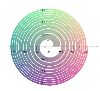
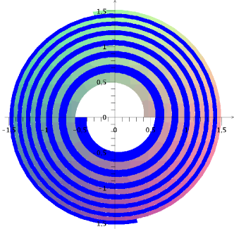
Figure 1. Numerical simulation of the simple spiral $\varphi_{A,B,\lambda,\delta,r}\colon(x,y)\mapsto(u,v)$ in Lemma 3.1.

Lemma 3.1 (Simple Spiral Lemma).

For any values $A>0,\,\,B>0,\,\,\lambda>0,\,\,\delta\geqslant 0,\,\,r\geqslant 0,$ the map

(1) $$\varphi_{A,B,\lambda,\delta,r}\colon{\rm R}(A,B)\to\mathbb{R}^{2},\,\,\,\,\,\,\,\,\,(x,y)\mapsto(u,v)$$

given by the formulas

(2) $$\begin{cases}u=\sqrt{\frac{I}{\pi}}\cos(2\pi\theta)\\ v=\sqrt{\frac{I}{\pi}}\sin(2\pi\theta),\end{cases}$$

where $I$ and $\theta$ are given by $I=y\lambda+r+\frac{x}{\lambda}(B\lambda+\delta)$ and $\theta=\frac{x}{\lambda}\mod 1$, satisfies the following properties:

1. $\varphi_{A,B,\lambda,\delta,r}$ is a symplectic embedding of ${\rm R}(A,B)$ into ${\rm B}^{2}(r)$, where the radius $r_{A}$ is given by $r_{A}=\sqrt{\frac{B\lambda+r+AB+\frac{A\delta}{\lambda}}{\pi}}.$

2. $\varphi_{A,B,\lambda,\delta,r}$ maps any subrectangle ${\rm R}(L,B)=(0,L)\times(0,B)$ for all $L\leqslant A,$ of ${\rm R}(A,B)$ into ${\rm B}^{2}(r_{L})$, where

   (3) $$r_{L}=\sqrt{\frac{B\lambda+r+LB+\frac{L\delta}{\lambda}}{\pi}}.$$

   (See Figure 1).

3. The image of $\varphi_{A,B,\lambda,\delta,r}$ avoids the closed ball $\overline{\textup{B}^{2}(\sqrt{r/\pi})}$.

4. Let $P$ be the closed subset of $\mathbb{R}^{5}\times\mathbb{R}^{5}\times\mathbb{R}^{5}$ :

   $$P=(\mathbb{R}^{*}_{+})^{5}\,\cup\Big{(}\underbrace{(\mathbb{R}^{*}_{+})^{4}}_{A,B,\lambda,\delta}\times\{r=0\}\Big{)}\,\cup\Big{(}\underbrace{(\mathbb{R}^{*}_{+})^{4}}_{A,B,\lambda,r}\times\{\delta=0\}\Big{)},$$

   where $\mathbb{R}^{*}_{+}$ denotes the set of strictly positive real numbers. Then the family $(\varphi_{A,B,\lambda,\delta,r})_{(A,B,\lambda,\delta,r)\in P}$ is smooth.

Proof.

Consider the symplectic maps:

(6) $$\left(\begin{array}[]{cc}\frac{1}{\lambda}&0\\ 0&\lambda\end{array}\right)\colon\mathbb{R}^{2}\to\mathbb{R}^{2},$$

(7) $$(\cdot,\cdot)+(0,r)\colon\mathbb{R}^{2}\to\mathbb{R}^{2},$$

(10) $$\left(\begin{array}[]{cc}1&0\\ B\lambda+\delta&1\end{array}\right)\colon\mathbb{R}^{2}\to\mathbb{R}^{2},$$

(11) $$\textup{projection onto}\,\,\mathbb{R}\times(\mathbb{R}/\mathbb{Z})\colon\mathbb{R}^{2}\to\mathbb{R}\times(\mathbb{R}/\mathbb{Z}).$$

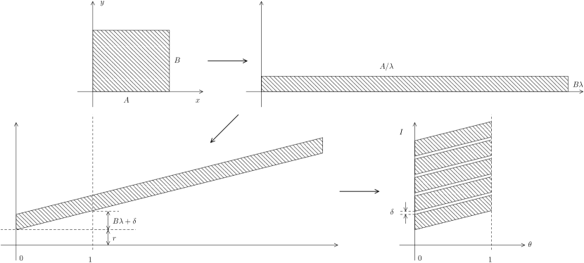
The composition of these maps gives the symplectomorphism depicted in Figure 2, and is expressed by the following formulas:

(12) $$\,\,\,\,\,\,\,\,\,\,\,(x,y)\stackrel{{\scriptstyle(\ref{map1})}}{{\longmapsto}}\Big{(}\frac{x}{\lambda},y\lambda\Big{)}\stackrel{{\scriptstyle(\ref{map2})}}{{\longmapsto}}\Big{(}\frac{x}{\lambda},y\lambda+r\Big{)}\stackrel{{\scriptstyle(\ref{map3})}}{{\longmapsto}}\Big{(}\frac{x}{\lambda},y\lambda+r+\frac{x}{\lambda}(B\lambda+\delta)\Big{)},$$

where each function in (12) is restricted to its domain in Figure 2 .

Figure 2. Domains and images of the transformations given by formulas (6), (7), (10), (11).

Then we compose the map (12) with symplectic polar coordinates $\mathbb{R}^{*}\times(\mathbb{R}/\mathbb{Z})\to\mathbb{R}^{2}\setminus\{(0,0)\}$, away from the singularity as in (2), and in this way obtain a symplectic embedding $\varphi_{A,B,\lambda,\delta,r}$ given in the statement of the lemma. The fact that $\varphi_{A,B,\lambda,\delta,r}$ is injective follows from $\delta\geqslant 0$ – see the Figure 2 – and the slope of the line in the third part of the figure is $B\lambda+\delta$. This can be also be easily checked from the formulas for $u$ and $v$. Finally, smoothness of the family follows from the fact that all transformations depend smoothly on the parameters in $P$. The singularity of the polar coordinates (2) is not included in the domain because the rectangles are open. ∎

4. Review of [4, Section 6]

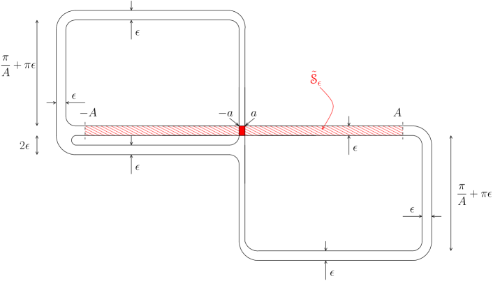
We need to use in the following sections the construction of a symplectic embedding given in [4, Section 6], and because it is essential for the proof, we review it next. It was proven therein that for sufficiently small fixed $\epsilon>0$ one can construct a symplectic immersion $i_{\epsilon}\colon\Sigma(\tilde{\epsilon})\hookrightarrow\mathbb{R}^{2}$ where $\tilde{\epsilon}:=100\epsilon$ as in Figure 3, with $a=\epsilon^{2}$. In particular, the double points of the immersion are concentrated in the small region $[-a,a]\times[-\epsilon/2,\epsilon/2]$.

Figure 3. The immersion $i_{\epsilon}\colon\Sigma(\tilde{\epsilon})\hookrightarrow\mathbb{R}^{2}$.

Consider a smooth cut-off function $\chi_{\epsilon}\colon\mathbb{R}\to[0,1]$ which is non decreasing on ${\mathbb{R}}^{-}$, non increasing on ${\mathbb{R}}^{+}$, $\chi_{\epsilon}\equiv 1$ on $[-a,\,a]$, $\chi_{\epsilon}\equiv 0$ on $\mathbb{R}\setminus[-A+\epsilon^{2},\,A-\epsilon^{2}]$, such that $|\chi^{\prime}_{\epsilon}(x)|\leqslant\frac{1}{A}+\epsilon$ for every $x\in\mathbb{R}$, and for every $x\in[-A+\frac{\epsilon}{2},\,A-\frac{\epsilon}{2}]$, one has that

(13) $$\biggl{\rvert}\chi_{\epsilon}(x)-\Big{(}1-\frac{|x|}{A}\Big{)}\biggr{\rvert}\leqslant\epsilon.$$

On $\mathbb{R}^{2}\times\mathbb{R}^{2}$ we define the smooth family of Hamiltonian functions

$$(\mathcal{H}_{\epsilon}(x_{1},y_{1},x_{2},y_{2}):=-\chi_{\epsilon}(x_{1})x_{2}\,\sqrt{\pi})_{\epsilon}$$

whose time-$1$ flows are given by the smooth family $(\Phi_{\epsilon})_{\epsilon}$ :

$$\,\,\,\,\,\,\,\,\,\,\Phi_{\epsilon}(x_{1},y_{1},x_{2},y_{2})=\Big{(}x_{1},\,\,y_{1}+\chi^{\prime}_{\epsilon}(x_{1})x_{2}\sqrt{\pi},\,\,x_{2},\,\,y_{2}+\chi_{\epsilon}(x_{1})\sqrt{\pi}\Big{)}.$$

Let ${\rm Q}(\sqrt{\pi})$ denotes the open square $(0,\sqrt{\pi})\times(0,\sqrt{\pi})$ and ${\rm R}(\sqrt{\pi},2\sqrt{\pi})$ be the open rectangle $(0,\sqrt{\pi})\times(0,2\sqrt{\pi})$. Let $\mathcal{S}_{\epsilon}$ be the connected subset of $\Sigma(\tilde{\epsilon})$ that is mapped to the horizontal strip $\widetilde{\mathcal{S}_{\epsilon}}=(-A,A)\times(-\frac{\epsilon}{2},\frac{\epsilon}{2})$ by the immersion $i_{\epsilon}$ (See Figure 3). We define $\mathcal{I}_{\epsilon}\colon\Sigma(\tilde{\epsilon})\times{\rm Q}(\sqrt{\pi})\to\mathbb{R}^{4}$ by

(14) $$\mathcal{I}_{\epsilon}(\sigma,\,b):=\begin{cases}\Phi_{\epsilon}(i_{\epsilon}(\sigma),b)&\text{ if }\sigma\in\mathcal{S}_{\epsilon};\\ (i_{\epsilon}(\sigma),b)&\text{ if }\sigma\notin\mathcal{S}_{\epsilon},\\ \end{cases}$$

which as shown in [4] is a symplectic embedding onto $\mathbb{R}^{2}\times{\rm R}(\sqrt{\pi},\,2\sqrt{\pi})$.

5. Embeddings into ${\rm B}^{4}(R)\times\mathbb{R}^{2(n-2)}$

The following is a smooth family version of the main statement in Hind and Kerman [3, Section 4.2].

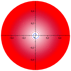
Figure 4. Numerical simulation of the embedding in Theorem 5.1 of a square of side $1$ into a ball of radius $1/\sqrt{\pi}$.

Theorem 5.1.

For any $\epsilon>0$, we let $\Sigma(\epsilon):=({\mathbb{R}}^{2}\setminus\sqrt{\epsilon}{\mathbb{Z}}^{2})/\sqrt{\epsilon}{\mathbb{Z}}^{2}$ be the scaling of $\Sigma$ with symplectic area $\epsilon$. There exist constants $\epsilon_{0}>0$, $c>0$, and a smooth family $({J}_{\epsilon})_{\epsilon\in(0,\epsilon_{0}]}$ of symplectic embeddings ${J}_{\epsilon}\colon\Sigma(\epsilon)\times{\rm B}^{2}(1)\hookrightarrow{\rm B}^{4}(\sqrt{3}+c\epsilon).$

Proof.

We will construct the embeddings explicitly, using spiral constructions.

Step 1 (A new embedding for $R(\sqrt{\pi},2\sqrt{\pi})$). We define $F:R(\sqrt{\pi},2\sqrt{\pi})\to{\mathbb{R}}^{2}$ to be the vertical analogue of the simple spiral

(15) $$\varphi_{A,B,\lambda,r,\delta},\,\,\textup{with}\,\,A=2\sqrt{\pi},\,\,\,B=\sqrt{\pi},\,\,\,\lambda=\epsilon,\,\,\,r=0,\,\,\,\delta=0$$

in Lemma 3.1 (and Figure 1). Precisely, we define

$$F:=\varphi_{A,B,\lambda,r,\delta}\circ R,$$

where $R$ is the rotation of angle $-\pi/2$ around the origin, followed by the translation of vector $(0,\sqrt{\pi})$.

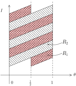
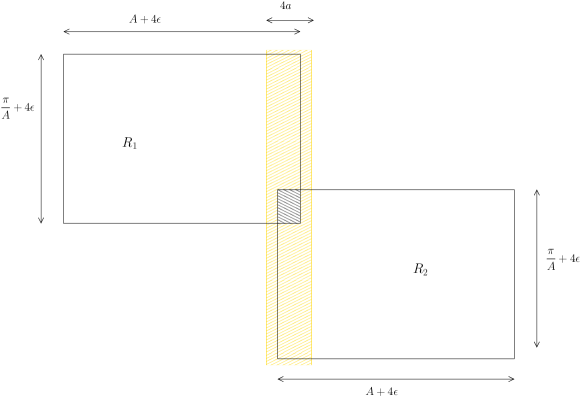
Step 2 (A new embedding of $D_{\epsilon}$). The construction of a new embedding $\Phi_{\epsilon}$ for $D_{\epsilon}$ is a bit more involved. The domain $D_{\epsilon}$ can be covered by two rectangles $R_{1},R_{2}$ (see Figure 5), and each rectangle will be sent to a spiral, in such a way that the spirals don’t overlap each other, and that there is enough space left in the image to properly glue the two spirals together.

Figure 5. Rectangles $R_{1},\,R_{2}$, and the central strip $E(4a)$.

We identify $R_{2}$ with the rectangle $R(A+4\epsilon,\tfrac{\pi}{A}+2\epsilon)$ and spiral it with the symplectic embedding $\varphi_{\tilde{A},B,\lambda,r,\delta}$, given by (1), where the parameters are :

(16) $$\,\,\,\,\,\,\,\,\,\,\,\tilde{A}=A+4\epsilon,\,\,\,\,\,\,\,B=\frac{\pi}{A}+4\epsilon,\,\,\,\,\,\,\,\lambda=\frac{\epsilon}{B},\,\,\,\,\,\,\,r=M\epsilon,\,\,\,\,\,\,\,\delta=\epsilon,$$

where the constant $M>0$ will be determined later. Thus we have a symplectic embedding $\beta_{2}\colon R_{2}\to\mathbb{R}^{2}$. Similarly, we have a symplectic embedding $\beta_{1}\colon R_{1}\to\mathbb{R}^{2}$ by rotating $R_{1}$ by the angle $\pi$ and translating it so that its lower right corner is at the origin $(0,0)$; we obtain $R(\tilde{A},B)$ and then we spiral it with a modified symplectic embedding $\tilde{\varphi}_{\tilde{A},B,\lambda,r,\delta}$, which is given as in Lemma 3.1, except that instead of $\theta=\frac{x}{\lambda}$ we use $\theta=\frac{x}{\lambda}+\frac{1}{2}$. See Figure 6.

Figure 6. Construction of the double spiral embedding

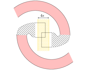
For $b>0$ we denote by $E(b)$ be the vertical strip $(-b/2,b/2)\times{\mathbb{R}}$. The final embedding $\Phi_{\epsilon}$ will be obtained by glueing the restrictions $\beta_{1}|_{R_{1}\setminus E(4\epsilon^{2})}$ and $\beta_{2}|_{R_{2}\setminus E(4\epsilon^{2})}$ to the central piece $W:=(R_{1}\cup R_{2})\cap E(4\epsilon^{2})$ (see Figure 7).

Figure 7. Gluing simple spirals in Step 1 of Theorem 5.1.

This can be done by sending $W$ inside the ball of radius $\sqrt{r/\pi}=\sqrt{M\epsilon/\pi}$, which is possible for $M$ large enough, since the area of $W$ is $\mathcal{O}(\epsilon^{2})$ (Lemma 3.1, part 3.)
Step 3 (Definition of $\mathcal{J}_{\epsilon}$). Let

$$\mathcal{J}_{\epsilon}\colon\Sigma(\epsilon)\times{\rm Q}(\sqrt{\pi})\to\mathbb{R}^{2}\times\mathbb{R}^{2}$$

be defined by $\mathcal{J}_{\epsilon}:=(\Phi_{\epsilon}\otimes F)\circ\mathcal{I}_{\epsilon}$, where $\mathcal{I}_{\epsilon}\colon\Sigma(\tilde{\epsilon})\times{\rm Q}(\sqrt{\pi})\to\mathbb{R}^{4}$ was defined in formula (14). We’ll write $(x_{1},y_{1},x_{2},y_{2})=\mathcal{I}_{\epsilon}(\sigma,b)$ and $(z_{1},z_{2})=\mathcal{J}_{\epsilon}(\sigma,b)$ and hence $z_{1}=\Phi_{\epsilon}(x_{1},y_{1})$ and $z_{2}=F(x_{2},y_{2})$. Our next goal is to show that there is some constant $c>0$, independent of $\epsilon,z_{1},z_{2}$, such that

(17) $$\mathcal{J}_{\epsilon}(\Sigma(\epsilon)\times{\rm Q}(\sqrt{\pi}))\subset{\rm B}^{4}(\sqrt{3}+c\epsilon),$$

and in order to do this, we will find upper estimates for $|z_{1}|$ and $|z_{2}|$.

Step 4 (The image of $\mathcal{J}_{\epsilon}$). In this step we will repeatedly use the formulas in (16). Consider the subrectangle $\hat{R}:={\rm R}(y_{2},A)=(0,y_{2})\times(0,A).$ Using the

Figure 8. Numerical approximation of $\Phi_{\epsilon}$ in Step 2 of proof of Theorem 5.1, before the gluing in Figure 7.

formulas for the parameters in (15) and formula (3) we obtain an inclusion

(18) $$F(\hat{R})\subset{\rm B}^{2}(r_{y_{2}}).$$

where

(19) $$r_{y_{2}}=\sqrt{\frac{\sqrt{\pi}\epsilon+0+\sqrt{\pi}y_{2}+0}{\pi}}=\sqrt{\frac{y_{2}+\epsilon}{\sqrt{\pi}}}.$$

Since $z_{2}\in\overline{F(\hat{R})}$, we get

(20) $$|z_{2}|\leqslant\sqrt{\frac{y_{2}+\epsilon}{\sqrt{\pi}}}.$$

Now we have two cases : (i) if $\sigma\notin\mathcal{S}_{\epsilon}$ then $0<y_{2}=b_{2}<\sqrt{\pi}$, and (ii) if $\sigma\in\mathcal{S}_{\epsilon}$ then $y_{2}=b_{2}+\chi_{\epsilon}(x_{1})\sqrt{\pi}$. Therefore $0<y_{2}<\sqrt{\pi}+\chi_{\epsilon}(x_{1})\sqrt{\pi}$, and hence the estimate (13) implies

(21) $$0<y_{2}\leqslant\sqrt{\pi}\Big{(}2-\frac{|x_{1}|}{A}+\epsilon\Big{)}.$$

It follows from putting together (20) and (21) that

(22) $$|z_{2}|^{2}\leqslant 2-\frac{|x_{1}|}{A}+\epsilon(1+1/\sqrt{\pi}).$$

This concludes the estimate for $|z_{2}|^{2}$.

Next we find an estimate for $|z_{1}|^{2}$. Recall that $(x_{1},y_{1})\in D_{\epsilon}$. If $(x_{1},y_{1})$ belongs to the central region $W$, then $\left|z_{1}\right|\leqslant{r/\pi}=\mathcal{O}(\epsilon)$. Otherwise, we may assume that $(x_{1},y_{1})$ lies in the rectangle $R_{2}$ (see Figure 5); the case $(x_{1},y_{1})\in R_{1}$ is symmetrically dealt with. Let us consider the subrectangle $R(x_{1},B)$; from (3) and (16) we get :

(23) $$|z_{1}| \leqslant \frac{1}{\sqrt{\pi}}\sqrt{\epsilon+M\epsilon+x_{1}\Big{(}\frac{\pi}{A}+4\epsilon\Big{)}+x_{1}\Bigl{(}\frac{\pi}{A}+4\epsilon\Bigr{)}}$$

$$\leqslant \sqrt{\frac{2x_{1}}{A}+\frac{\epsilon(1+M+8x_{1})}{\pi}}.$$

It follows from (23) that there exists a constant $C<\infty$ (recall that $0<x_{1}<A+4\epsilon$) such that

(24) $$\frac{|z_{1}|^{2}}{2}\leqslant\frac{|x_{1}|}{A}+C\epsilon,$$

and in particular

(25) $$\frac{\left|z_{1}\right|^{2}}{2}\leqslant 1+\tilde{C}\epsilon,$$

where $\tilde{C}=C+4/A$. Hence from (22) and (24) we get that

(26) $$\frac{|z_{1}|^{2}}{2}+|z_{2}|^{2}\leqslant 2+(1+C+1/\sqrt{\pi})\epsilon.$$

Adding (25) we obtain that :

$$|z_{1}|^{2}+|z_{2}|^{2}\leqslant 3+c\epsilon,$$

where $c:=1+2C+1/\sqrt{\pi}+4/A$ is a constant independent of $\epsilon,z_{1},z_{2}$. Hence we get (17), which concludes the proof of the theorem. ∎

The following corresponds to [3, Theorem 1.3] for smooth families.

Theorem 5.2.

Let $n\geqslant 3$. There exist constants $C,C^{\prime}>0$ and a smooth family of symplectic embeddings

$$i_{S,\,R}\colon{\rm B}^{2}(1)\times{\rm B}^{2(n-1)}(S)\hookrightarrow{\rm B}^{4}(R)\times\textup{B}^{2(n-2)}({\textstyle\frac{CS^{2}}{\sqrt{R-\sqrt{3}}}}),$$

where $(S,R)$ vary in the open set

(27) $$\{(S,R)\in{\mathbb{R}}^{2}\,\,|\qquad S>0,\quad\sqrt{3}<R<\sqrt{3}+C^{\prime}S^{2}\}.$$

Proof.

The proof is essentially identical to that of [4, Theorem 6.4]. Consider the embedding $i_{T}\colon{\rm B}^{2(n-1)}(T)\hookrightarrow\Sigma\times{\rm B}^{2(n-2)}(10T^{2})$, $T>{\textstyle\frac{1}{3}}$ in Lemma 2.2. For $\epsilon>0$, let $\tau_{\sqrt{\epsilon}}:{\mathbb{R}}^{2(n-1)}\to{\mathbb{R}}^{2(n-1)}$ be the dilation $\tau_{\sqrt{\epsilon}}(x)=\sqrt{\epsilon}x$. The corresponding quotient map $\bar{\tau}_{\sqrt{\epsilon}}$ maps $\Sigma\times{\mathbb{R}}^{2(n-2)}$ to $\Sigma(\epsilon)\times{\mathbb{R}}^{2(n-2)}$, The map $\bar{\tau}_{\sqrt{\epsilon}}\circ i_{T}\circ(\tau_{\sqrt{\epsilon}})^{-1}$ is a symplectic embedding of $\tau_{\sqrt{\epsilon}}({\rm B}^{2(n-1)}(T))={\rm B}^{2(n-1)}(\sqrt{\epsilon}T)$ into $\bar{\tau}_{\sqrt{\epsilon}}(\Sigma\times{\rm B}^{2(n-2)}(10T^{2}))=\Sigma(\epsilon)\times{\rm B}^{2(n-2)}(10\sqrt{\epsilon}T^{2}))$. Of course, as $T>\frac{1}{3}$ varies, the corresponding family of embeddings is smooth. By composing with the embeddings given by Theorem 5.1, we end up with a smooth family of symplectic embeddings :

$${\rm B}^{2}(1)\times{\rm B}^{2(n-1)}(\sqrt{\epsilon}T)\hookrightarrow{\rm B}^{4}(\sqrt{3}+c\epsilon)\times\textup{B}^{2(n-2)}(10\sqrt{\epsilon}T^{2}),$$

$$T>1/3,\quad\epsilon>0.$$

The conclusion follows by the smooth parameter change $(S,R):=(\sqrt{\epsilon}T,\sqrt{3}+c\epsilon)$, with $C=10\sqrt{c}$ and $C^{\prime}=9c$. ∎

6. Proof of Theorem 1.2

From [3, Theorem 1.1] we know that if $0<R<\sqrt{3}$ there are no symplectic embeddings of ${\rm B}^{2}(1)\times{\rm B}^{2(n-1)}(S)$ into ${\rm B}^{4}(R)\times\mathbb{R}^{2(n-2)}$ when $S$ is large. Therefore, it remains to prove that ${\rm B}^{2}(1)\times{\mathbb{R}}^{2(n-1)}$ symplectically embeds into ${\rm B}^{4}(\sqrt{3})\times\mathbb{R}^{2(n-2)}$.

The proof is analogous to the proof of [4, Theorem 3.3]. By Theorem 5.2 there exist some constants $C,C^{\prime}>0$ and a smooth family of symplectic embeddings $i_{S,\,R}\colon{\rm B}^{2}(1)\times{\rm B}^{2(n-1)}(S)\hookrightarrow{\rm B}^{4}(R)\times\textup{B}^{2(n-2)}({\textstyle\frac{CS^{2}}{\sqrt{R-\sqrt{3}}}}),$ where $(S,R)$ is in the region $A$ of $(S,R)\in{\mathbb{R}}^{2}$ such that $S>0$ and $\sqrt{3}<R<\sqrt{3}+C^{\prime}S^{2}$. For all $\epsilon>0$ small enough we may define a smooth family of symplectic embeddings

(28) $$\phi_{\epsilon}\colon{\rm B}^{2}(1-\epsilon)\times{\rm B}^{2(n-1)}(1/\epsilon)\hookrightarrow{\rm B}^{4}(\sqrt{3})\times\textup{B}^{2(n-2)}\Bigl{(}\frac{3^{-1/4}C}{\sqrt{\epsilon^{5}(1-\epsilon)}}\Bigr{)}$$

by $\phi_{\epsilon}(x):=(\frac{\sqrt{3}}{R})i_{S,R}(\frac{R}{\sqrt{3}}x)$ with $S=\frac{1}{\epsilon(1-\epsilon)}$ and $R=\frac{\sqrt{3}}{1-\epsilon}$. We apply Theorem 2.1 to the family (28) and get a symplectic embedding ${\rm B}^{2}(1)\times\mathbb{R}^{2(n-1)}\hookrightarrow{\rm B}^{4}(\sqrt{3})\times\mathbb{R}^{2(n-2)}.$

Acknowledgements. We thank Helmut Hofer for helpful discussions. AP was partly supported by NSF Grant DMS-0635607, an NSF CAREER Award DMS-1055897, a J. Tinsley Oden Faculty Fellowship at the Institute for Computational Engineering and Sciences (ICES) in Austin, a Leibniz Fellowship from Oberwolfach, Spain Ministry of Science Grant Sev-2011-0087. VNS is partially supported by the Institut Universitaire de France, the Lebesgue Center (ANR Labex LEBESGUE), and the ANR NOSEVOL grant. He gratefully acknowledges the hospitality of the IAS.

Álvaro Pelayo
School of Mathematics
Institute for Advanced Study
Einstein Drive
Princeton, NJ 08540 USA

Washington University, Mathematics Department
One Brookings Drive, Campus Box 1146
St Louis, MO 63130-4899, USA.
E-mail: apelayo@math.wustl.edu
E-mail: apelayo@math.ias.edu

San Vũ Ngọc
Institut Universitaire de France

Institut de Recherches Mathématiques de Rennes
Université de Rennes 1, Campus de Beaulieu
F-35042 Rennes cedex, France
E-mail: san.vu-ngoc@univ-rennes1.fr

References

• [1] I. Ekeland and H. Hofer: Symplectic topology and Hamiltonian dynamics. Math. Z. 200 (1989) 355–378.
• [2] L. Guth: Symplectic embeddings of polydisks. Invent. Math. 172 (2008) 477–489.
• [3] R. Hind and E. Kerman: New obstructions to symplectic embeddings. arXiv:0906.4296v2.
• [4] Á. Pelayo and S. Vũ Ngọc: The Hofer question on intermediate symplectic capacities. arXiv:1210.1537v3.
• [5] F. Schlenk: Embedding Problems in Symplectic Geometry. de Gruyter Expositions in Mathematics, vol. 40. Walter de Gruyter, Berlin (2005).