A geometric study of Wasserstein spaces: ultrametrics

Abstract

We study the geometry of the space of measures of a compact ultrametric space $X$, endowed with the $L^{p}$ Wasserstein distance from optimal transportation. We show that the power $p$ of this distance makes this Wasserstein space affinely isometric to a convex subset of $\ell^{1}$. As a consequence, it is connected by $\frac{1}{p}$-Hölder arcs, but any $\alpha$-Hölder arc with $\alpha>\frac{1}{p}$ must be constant.

This result is obtained via a reformulation of the distance between two measures which is very specific to the case when $X$ is ultrametric; however thanks to the Mendel-Naor Ultrametric Skeleton it has consequences even when $X$ is a general compact metric space. More precisely, we use it to estimate the size of Wasserstein spaces, measured by an analogue of Hausdorff dimension that is adapted to (some) infinite-dimensional spaces. The result we get generalizes greatly our previous estimate that needed a strong rectifiability assumption.

The proof of this estimate involves a structural theorem of independent interest: every ultrametric space contains large co-Lipschitz images of regular ultrametric spaces, i.e. spaces of the form $\{1,\dots,k\}^{\mathbb{N}}$ with a natural ultrametric.

We are also lead to an example of independent interest: a space of positive lower Minkowski dimension, all of whose proper closed subsets have vanishing lower Minkowski dimension.

1 Introduction

Given a metric space $X$, that we shall always assume to be compact, one can define its $L^{p}$ Wasserstein space $\mathop{\mathscr{W}}\nolimits_{p}(X)=(\mathop{\mathscr{missing}}{P}\nolimits(X),\mathop{\mathrm{W}}\nolimits_{p})$ as the set of its Borel probability measures $\mathop{\mathscr{missing}}{P}\nolimits(X)$ endowed with a distance $\mathop{\mathrm{W}}\nolimits_{p}$ defined using optimal transportation (see below for precise definitions). In some sense, $\mathop{\mathscr{W}}\nolimits_{p}(X)$ can be thought of as a geometric measure theory analogue of $L^{p}$ space, although its geometry is finely governed by the geometry of $X$ as $\mathop{\mathrm{W}}\nolimits_{p}$ involves the metric on $X$ in a crucial way; in particular, the great variety of metric spaces induces a great variety of Wasserstein spaces. As a consequence, the natural affine structure of $\mathop{\mathscr{missing}}{P}\nolimits(X)$ (i.e., its affine structure as a convex in the dual space of continuous functions) is in general only loosely related to the geometric structure of $\mathop{\mathrm{W}}\nolimits_{p}$.

The links between optimal transportation and geometry have been the object of a lot of studies in the past decade. In a series of papers we try to understand what kind of geometric information on $\mathop{\mathscr{W}}\nolimits_{p}(X)$ can be obtained from given geometric information on $X$. We considered for example isometry groups and embeddability questions when $X$ is a Euclidean space [Klo10] or, with Jérôme Bertrand, a Hadamard space [BK12], and the size of $\mathop{\mathscr{W}}\nolimits_{p}(X)$ when $X$ is (close to be) a compact manifold [Klo12].

Here we consider the case when $X$ is a compact ultrametric space, i.e. satisfies the following strengthening of the triangular inequality:

$$d(x,z)\leqslant\max(d(x,y),d(y,z)).$$

Examples of compact ultrametric spaces include notably the set of $p$-adic integers $\mathbb{Z}_{p}$ or more generally the set $\{1,\dots,k\}^{\mathbb{N}}$ of infinite words on an alphabet with $k$ letters, endowed with the distance $d(\bar{x},\bar{y})=q^{-\min\{i,x_{i}\neq y_{i}\}}$ where $q>1$ and $\bar{x}=(x_{1},x_{2},\dots)$, $\bar{y}=(y_{1},y_{2},\dots)$. We shall call these examples regular ultrametric spaces and denote them by $Y(k,q)$.

1.1 Embedding in snowflaked $\ell^{1}$

Ultrametric spaces are in some sense the simplest spaces in which to do optimal transportation, thanks to the very strong structure given by the ultrametric inequality. We are therefore able to give a very concrete description of $\mathop{\mathscr{W}}\nolimits_{p}(X)$.

.

If $X$ is a compact ultrametric space, then $(\mathop{\mathscr{missing}}{P}\nolimits(X),\mathop{\mathrm{W}}\nolimits_{p}^{p})$ is affinely isometric to a convex subset of $\ell^{1}$.

Another way to state this result is to say that $\mathop{\mathscr{W}}\nolimits_{p}(X)$ is affinely isometric to a convex subset of $\ell^{1}$ endowed with the “snowflaked” metric $\|\cdot\|_{1}^{1/p}$. Note that the existence of such an embedding, both affine and geometrically meaningful, of $\mathop{\mathscr{W}}\nolimits_{p}(X)$ into a Banach space seems to be quite exceptional; the closest case I know of is $\mathop{\mathscr{W}}\nolimits_{p}(\mathbb{R})$, which is isometric to a subset of increasing functions in $L^{p}([0,1])$, but even there the isometry is not affine. In fact, the absence of correlation between the affine structure of $\mathop{\mathscr{missing}}{P}\nolimits(X)$ and the geometry of $\mathop{\mathrm{W}}\nolimits_{p}$ is an important reason for the relevance of Wasserstein spaces, as the very fact that geodesics in the space of measures (when they exist) are usually not affine lines made it possible to define a new convexity assumption that turned out to be very successful, see notably [McC97]. In this sense, Theorem 1.1 is a negative result: when $X$ is ultrametric there is little more to $\mathop{\mathscr{W}}\nolimits_{p}(X)$ than to $\mathop{\mathscr{missing}}{P}\nolimits(X)$, as far as we are concerned with notions which are affine in nature (e.g. convexity). We shall see, however, that this result has nice consequences.

As is well-known, snowflaked metrics are geometrically very disconnected (all rectifiable curves are constant) and this affects the geometric connectivity of Wasserstein space.

.

If $X$ is a compact ultrametric space, $\mathop{\mathscr{W}}\nolimits_{1}(X)$ is a geodesic space, and for $p>1$, $\mathop{\mathscr{W}}\nolimits_{p}(X)$ is connected by $\frac{1}{p}$-Hölder arcs but any $\alpha$-Hölder arc with $\alpha>\frac{1}{p}$ must be constant.

1.2 Size estimates

While their strong structural properties make ultrametric spaces feel quite easy to deal with, they also happen to be ubiquitous, as shown by the ultrametric skeleton Theorem of Mendel and Naor [MN13a, MN13b]: very roughly, any metric space contains large almost ultrametric parts. This powerful result enables us to control very precisely the size of very general Wasserstein spaces.

.

Given any compact metric space $X$ (not necessarily ultrametric), we have

$$\mathop{\mathrm{missing}}{crit}\nolimits_{\mathscr{P}}\mathop{\mathscr{W}}\nolimits_{p}(X)\geqslant\dim X.$$

Here, $\dim$ denotes the Hausdorff dimension, and $\mathop{\mathrm{missing}}{crit}\nolimits_{\mathscr{P}}$ is the power-exponential critical parameter introduced in [Klo12], which is an extension of Hausdorff dimension that distinguishes some infinite-dimensional spaces. This bi-Lipschitz invariant is constructed simply by replacing the terms $\varepsilon^{s}$ by $\exp(-\varepsilon^{-s})$ in the definition of Hausdorff dimension. In particular, the above result implies that to cover $\mathop{\mathscr{W}}\nolimits_{p}(X)$ one needs at least very roughly $\exp(\varepsilon^{-\dim X})$ balls of radius $\varepsilon$.

.

It is in fact possible to give an elementary proof of Theorem 1.2 that does not use ultrametric spaces. We shall give such a proof in Section 6, but we feel the ultrametric proof has its own worth as it shows a way to use the ultrametric skeleton theorem and could apply more generally (notably to estimate the size of other large spaces, as spaces of closed subsets, spaces of Hölder functions, etc.).

In fact, the non-ultrametric proof was only found some time after submission of the first version of this article, and the ultrametric skeleton theorem played a key role in the author’s mind when thinking about the whole issue.

As we proved in [Klo12] that $\mathop{\mathrm{missing}}{crit}\nolimits_{\mathscr{P}}\mathop{\mathscr{W}}\nolimits_{p}(X)$ is at most the upper Minkowski dimension $\mathop{\operatorname{\overline{M}-dim}}\nolimits X$ of $X$, the following results follow at once from Theorem 1.2.

.

Let $X$ be any compact metric space (not necessarily ultrametric); if $\dim X=\mathop{\operatorname{\overline{M}-dim}}\nolimits X=d$, then $\mathop{\mathrm{missing}}{crit}\nolimits_{\mathscr{P}}\mathop{\mathscr{W}}\nolimits_{p}(X)=d$.

This greatly generalizes two of the main results of [Klo12], focused on $p=2$ and where either instead of $\dim X=d$ we had to assume the much stronger assumption that $X$ contains a bi-Lipschitz image of $[0,1]^{d}$, or we could only conclude a much weaker lower bound on the size of $\mathop{\mathscr{W}}\nolimits_{2}(X)$ (even weaker than $\mathop{\mathrm{missing}}{crit}\nolimits_{\mathscr{P}}\mathop{\mathscr{W}}\nolimits_{2}(X)>0$).

.

Let $X,X^{\prime}$ be two compact metric spaces. If $\dim X>\mathop{\operatorname{\overline{M}-dim}}\nolimits X^{\prime}$, then there is no bi-Lipschitz embedding $\mathop{\mathscr{W}}\nolimits_{p}(X)\to\mathop{\mathscr{W}}\nolimits_{p^{\prime}}(X^{\prime})$, for any $p,p^{\prime}\in[1,\infty)$.

Let us also note that the Mendel-Naor ultrametric skeleton Theorem readily implies that for all $\varepsilon>0$, $\mathop{\mathscr{W}}\nolimits_{p}(X)$ contains a subset $S$ with $\mathop{\mathrm{missing}}{crit}\nolimits_{\mathscr{P}}S\geq(1-\varepsilon)\dim X$ that embeds in an ultrametric space with distortion $O(1/\varepsilon)$.

It would be more natural to replace the inequality on dimensions in Theorem 1.2 by $\dim X>\dim Y$, but our method cannot give that stronger statement. This seems inevitable since the Hausdorff dimension of $X$ gives no upper bound on the critical parameter of its Wasserstein spaces.

.

There is an ultrametric space $X$ such that $X$ is countable (in particular $\dim X=0$) but $\mathop{\mathrm{missing}}{crit}\nolimits_{\mathscr{P}}\mathop{\mathscr{W}}\nolimits_{p}(X)=+\infty$ for all $p$.

1.3 Structure of ultrametric space

In addition to the Mendel-Naor theorem, one important ingredient in the first proof of Theorem 1.2 is a structural result that seems of interest in itself, according to which every compact ultrametric space contains (in a weak sense) a large regular part, which is easier to deal with.

.

Given any compact ultrametric space $X$ and any $s<\dim X$, there is a regular ultrametric space $Y=Y(k,q)$ of Hausdorff dimension at least $s$ and a co-Lipschitz map $\varphi:Y\to X$.

By a co-Lipschitz map we mean that for some $c>0$ and all $a,b\in Y$ one has

$$d(\varphi(a),\varphi(b))\geqslant c\cdot d(a,b).$$

This shows that, a bit like ultrametric spaces are ubiquitous in metric spaces, regular ultrametrics are ubiquitous in ultrametrics (and therefore in metric spaces). The fact that we only obtain a co-Lipschitz map is a strong limitation, but this is sufficient for our present purpose.

1.4 Organization of the article

In the next section, we introduce briefly some classical definitions and facts concerning Wasserstein spaces, ultrametric spaces and we recall some properties of critical parameters. In Section 3, we prove Theorem 1.1 and corollary 1.1. Section 4 is devoted the purely ultrametric Theorem 1.3, while Sections 5 and 6 give the two proofs of Theorem 1.2. Last, Section 7 gives two examples motivating the dimension hypothesis in Theorem 1.2, notably proving Proposition 1.2.

2 Preliminaries

2.1 Wasserstein spaces

We limit ourselves in this short presentation to the case of a compact metric spaces $X$ whose distance is denoted by $d$. The set of Borel probability measures $\mathop{\mathscr{missing}}{P}\nolimits(X)$ is naturally endowed with a set of “Wasserstein” distances that echo the distance of $X$: for any $p\in[1,+\infty)$, one sets

$$\mathop{\mathrm{W}}\nolimits_{p}(\mu,\nu)=\left(\inf_{\Pi\in\Gamma(\mu,\nu)}\int_{X\times X}d(a,b)^{p}\,\Pi(\mathrm{d}a\,\mathrm{d}b)\right)^{\frac{1}{p}}$$

where $\Gamma(\mu,\nu)$ is the set of transport plans, or coupling of $(\mu,\nu)$, that is to say the set of measures $\Pi$ on $X\times X$ that projects on each factor as $\mu$ and $\nu$:

$$\Pi(A\times X)=\mu(A),\quad\Pi(X\times B)=\nu(B)\quad\forall\mbox{ Borel }A,B\subset X.$$

In other words, a transport plan specifies a way of allocating mass distributed according to $\mu$ so that it ends up distributed according to $\nu$; its $L^{p}$ cost

$$c_{p}(\Pi):=\inf_{\Pi\in\Gamma(\mu,\nu)}\int_{X\times X}d(a,b)^{p}\,\Pi(\mathrm{d}a\,\mathrm{d}b)$$

is the total cost of this allocation if one assumes that allocating a unit of mass from a point to a point $d$ away costs $d^{p}$, and $\mathop{\mathrm{W}}\nolimits_{p}(\mu,\nu)^{p}$ is the least possible cost of a transport plan.

It is easily proved (see e.g. [Vil09] for this and much more) that the infimum is realized by what is then called an optimal transport plan, that $\mathop{\mathrm{W}}\nolimits_{p}$ is indeed a distance and that it metricizes the weak topology. We shall denote by $\mathop{\mathscr{W}}\nolimits_{p}$ the metric space $(\mathop{\mathscr{missing}}{P}\nolimits(X),\mathop{\mathrm{W}}\nolimits_{p})$ and call it the ($L^{p}$) Wasserstein space of $X$.

We shall need very little more from the theory of optimal transportation, let us only state two further facts.

First, an easy consequence of “cyclical monotonicity” is that if $X$ is a metric tree (or its completion), $e$ is an edge of $X$, $\Pi$ is an optimal transport plan between measures $\mu,\nu\in\mathop{\mathscr{W}}\nolimits_{p}(X)$ supported outside $e$, and $X_{1},X_{2}$ are the connected components of $X\setminus e$, then

$$\Pi(X_{1}\times X_{2})=\max(\mu(X_{1})-\nu(X_{1}),0);$$

in other words, no more mass is moved through an edge than strictly necessary.

Second, the concept of displacement interpolation shall prove convenient. If $X$ is a geodesic space, $\mu,\nu\in\mathop{\mathscr{W}}\nolimits_{p}(X)$ and $\Pi$ is an optimal transport plan (implicitly, for the cost $c_{p}$ and from $\mu$ to $\nu$), then it is known that there is a probability measure $\pi$ on the set of constant speed geodesics $[0,1]\to X$ such that if one draws a random geodesic $\gamma$ with law $\pi$, the random pair $(\gamma(0),\gamma(1))$ of its endpoints has law $\Pi$. In other words, if $e_{t}:\gamma\mapsto\gamma(t)$ is the specialization map, $\Pi=(e_{0},e_{1})_{\#}\pi$. The measure $\pi$ is called an optimal dynamical transport plan. The interest of this description is that $\mathop{\mathscr{W}}\nolimits_{p}(X)$ is geodesic, and all its geodesics have the form $(e_{t\#}\pi)_{t\in[0,1]}$ for some optimal dynamical transport plan $\pi$.

Now, if $X$ is a metric tree, let say that two geodesics $\gamma_{1}$, $\gamma_{2}$ are antagonist if they both follow some edge $e$, in opposite directions. Then an optimal dynamical plan $\pi$ between any two measures is supported on a set without any pair of antagonist geodesics. This is of course closely linked to the cyclical monotonicity.

2.2 Critical parameters

Critical parameters where introduced in [Klo12] as bi-Lipschitz invariants similar to Hausdorff dimension but that can distinguish between some infinite-dimensional spaces, notably many Wasserstein spaces.

We shall not recall their construction here, but only a few facts that we shall use in the sequel. First, to define a critical parameter one needs a so-called scale, a family of functions playing the role played by $(r\mapsto r^{s})$ in the definition of Hausdorff dimension. We restrict here to the power-exponential scale $\mathscr{P}=(r\mapsto\exp(-1/r^{s}))_{s>0}$ and denote the corresponding critical parameter by $\mathop{\mathrm{missing}}{crit}\nolimits_{\mathscr{P}}$.

Then Frostman’s Lemma (see e.g. [Mat95]) gives a characterization of $\mathop{\mathrm{missing}}{crit}\nolimits_{\mathscr{P}}$, from which we extract the following conditions:

• if $\mathop{\mathrm{missing}}{crit}\nolimits_{\mathscr{P}}>s$ then there is $\mu\in\mathop{\mathscr{missing}}{P}\nolimits(X)$ and $C>0$ such that for all $x\in X$ and all $r>0$, $\mu(B(x,r))\leq C\exp(-1/r^{s})$;

• if there is a measure $\mu\in\mathop{\mathscr{missing}}{P}\nolimits(X)$ as above, then $\mathop{\mathrm{missing}}{crit}\nolimits_{\mathscr{P}}\geq s$.

In other words, $X$ has large critical parameter if it supports a very spread out measure. $\mathop{\mathrm{missing}}{crit}\nolimits_{\mathscr{P}}X$ is zero when $X$ has finite Hausdorff dimension, but turns out to be non-zero for many interesting infinite-dimensional spaces.

The second important fact is that $\mathop{\mathrm{missing}}{crit}\nolimits_{\mathscr{P}}$ can only increase under co-Lipschitz maps: if $f:Y\mapsto X$ satisfies $d(f(a),f(b))\geq c\cdot d(a,b)$ for some $c>0$ and all $a,b\in Y$, then $\mathop{\mathrm{missing}}{crit}\nolimits_{\mathscr{P}}(X)\geq\mathop{\mathrm{missing}}{crit}\nolimits_{\mathscr{P}}(Y)$. To prove lower bounds on critical parameters, our strategy will be to find in our space of interest co-Lipschitz images of spaces supporting a well spread-out measure.

To do that, we will need spaces on which such measures are easy to construct. We shall use the Banach cubes

$$\mathop{\mathrm{missing}}{BC}\nolimits((a_{n})_{n}):=\left\{(x_{n})\in\ell^{1}\,\middle|\,0\leq x_{n}\leq a_{n}\,\forall n\in\mathbb{N}\right\}$$

defined for any $\ell^{1}$ positive sequence $(a_{n})$. In [Klo12], $\mathop{\mathrm{missing}}{BC}\nolimits((a_{n})_{n})$ was denoted $\mathop{\mathrm{missing}}{BC}\nolimits([0,1],1,(a_{n})_{n})$ as a more general family of Banach cubes was defined. We have

$$\mathop{\mathrm{missing}}{crit}\nolimits_{\mathscr{P}}\mathop{\mathrm{missing}}{BC}\nolimits((n^{-\alpha}))=\frac{1}{\alpha-1}$$ (1)

for all $\alpha>1$; we shall only give a sketch of the proof, as it follows the same lines as the proof of the Hilbertian version of this estimate, given in full details in [Klo12] (section 4, see also Proposition 8.1 page 232).

Sketch of proof of (1).

The upper bound is obtained by bounding the upper Minkowski critical parameter, i.e. by bounding from above the number of balls of radius $\varepsilon$ needed to cover $\mathop{\mathrm{missing}}{BC}\nolimits((n^{-\alpha}))$. Let $L=L(\varepsilon/2)$ be the first integer such that

$$\sum_{n>L}n^{-\alpha}\leq\frac{\varepsilon}{2}$$

and, for each $n\leq L$, consider a minimal set of points $(x^{i}_{n})_{i}$ on $[0,n^{-\alpha}]$ such that every point of this interval is at distance at most $\varepsilon/(Cn\log^{2}n)$ of one of the $x^{i}_{n}$, where $C$ is such that $\sum_{1}^{\infty}(Cn\log^{2}n)^{-1}\leq 1/2$. Then, any point $\bar{x}=(x_{1},x_{2},\dots)\in\mathop{\mathrm{missing}}{BC}\nolimits((n^{-\alpha}))$ is a distance at most $\varepsilon$ from one of the points

$$(x_{1}^{i_{1}},x_{2}^{i_{2}},\dots,x_{L}^{i_{L}},0,0,\dots)$$

Then, an estimate of the number of such points shows that

$$\mathop{\mathrm{missing}}{crit}\nolimits_{\mathscr{P}}\mathop{\mathrm{missing}}{BC}\nolimits((n^{-\alpha}))\leq\frac{1}{\alpha-1}.$$

The lower bound is obtained using Frostman’s Lemma. We consider the uniform probability measure $\lambda_{n}$ on $[0,n^{-\alpha}]$ and the measure $\mu:=\otimes_{n}\lambda_{n}$ on $\mathop{\mathrm{missing}}{BC}\nolimits((n^{-\alpha}))$. Then, one can prove that for all $\beta<(\alpha-1)^{-1}$, there is a constant $C$ such that for all $\bar{x}\in\mathop{\mathrm{missing}}{BC}\nolimits((n^{-\alpha}))$ and all $r\leq 1$,

$$\log\mu(B(\bar{x},r))\leq-C\frac{1}{r^{\beta}}$$

(see pages 217-218 in [Klo12]). Frostman’s Lemma (Proposition 3.4 of [Klo12]) then ensures

$$\mathop{\mathrm{missing}}{crit}\nolimits_{\mathscr{P}}\mathop{\mathrm{missing}}{BC}\nolimits((n^{-\alpha}))\geq\frac{1}{\alpha-1}.$$

∎

2.3 Ultrametric spaces

According to the Ultrametric skeleton Theorem [MN13a, MN13b], given any compact metric space $X$ and any $s<\dim X$, there is an ultrametric space $X^{\prime}$ of dimension at least $s$ and a bi-Lipschitz embedding $X^{\prime}\to X$ (moreover, the distortion of this bi-Lipschitz embedding is $O(\dim X-s)^{-1})$). This simply stated result is very powerful, see [Nao12].

The other, older and classical fact we shall need about ultrametric spaces is their description in terms of trees (see e.g. [Nao12] Section 8.1 or [GNS00]).

By a tree we mean a simple graph $T$ with vertex set $V$ and edge set $E$, which is connected and without cycle; it can be infinite but is assumed to be locally finite. A tree is rooted if it has a distinguished vertex $o$, which is not a leaf, and called the root. A vertex $v\neq o$ has a unique parent $v^{*}$, defined as the neighbor of $v$ closer to $o$ than $v$; $v$ is then said to be a child of $v^{*}$. Each edge has a natural orientation, from parent to child: $(v^{*}v)$ is said to be a positive edge. A height function is a function $h:V\to[0,+\infty)$ that is decreasing: $h(v)<h(v^{*})$ for all $v\neq o$ (note that our trees have the root on top). A synchronized rooted tree (SRT for short) is a rooted tree endowed with a height function such that for any maximal (finite or infinite) oriented path $o,v_{1},v_{2},\dots$, we have $\lim h(v_{n})=0$ (in particular, all leaves have height $0$). The metric realization of a SRT $T$ is the metric space obtained by taking a segment of length $h(x)-h(y)$ for each positive edge $(xy)$ and gluing them according to $T$. It is still denoted by $T$, and the height function can be extended linearly on edges and continuously to the metric completion $\bar{T}$ of $T$; this extension is still denoted by $h$. By construction, $h^{-1}(0)$ is the union of all leafs of $T$ and of $\bar{T}\setminus T$. It is not hard to check that $h^{-1}(0)$, endowed with the restriction of the metric of $\bar{T}$, is ultrametric. We can now state the description alluded to above.

Any compact ultrametric space can be isometrically identified with the level $h^{-1}(0)$ of the completion of a metric SRT $T$.

For each vertex $v$ of $T$, the set of points in $X$ that can be reached by an oriented path from $v$ is a metric ball of $X$, denoted by $X_{v}$ and of diameter $2h(v)$. All balls of $X$ are of the form $X_{v}$ for some $v$, e.g. $X=X_{o}$.

The proof of the above folkloric fact is not difficult, and can be found up to little notational twists in the references cited above: one simply use the ultrametric inequality to partition $X$ into maximal proper balls, which will be identified with the children of $o$, and then proceed recursively.

3 $\ell^{1}$ coordinates

The goal of this Section is to prove Theorem 1.1: given a compact ultrametric space $X$ and $p\in[1,\infty)$, we want to construct an affine isometry from $(\mathop{\mathscr{missing}}{P}\nolimits(X),\mathop{\mathrm{W}}\nolimits_{p}^{p})$ to a convex subset of $\ell^{1}$, that is a map $\varphi:\mathop{\mathscr{missing}}{P}\nolimits(X)\to\ell^{1}$ with convex image and such that

$$\varphi(t\mu+(1-t)\nu)=t\varphi(\mu)+(1-t)\varphi(\nu)\quad\forall\mu,\nu\in\mathop{\mathscr{missing}}{P}\nolimits(X),\forall t\in[0,1]$$

and

$$\|\varphi(\mu)-\varphi(\nu)\|_{1}=\mathop{\mathrm{W}}\nolimits_{p}(\mu;\nu)^{p}\quad\forall\mu,\nu\in\mathop{\mathscr{missing}}{P}\nolimits(X).$$

Up to coefficients, this map is simply constructed by mapping a measure to the collection of masses it gives to balls of $X$.

3.1 A formula for the Wasserstein distance

Let $T$ be a metric SRT such that $X=h^{-1}(0)\subset\bar{T}$ as explained in §2.3. Then $\mathop{\mathscr{missing}}{P}\nolimits(X)$ is the subset of $\mathop{\mathscr{missing}}{P}\nolimits(\bar{T})$ made of measures concentrated on $X$, and $\mathop{\mathrm{W}}\nolimits_{p}$ is the restriction to $\mathop{\mathscr{missing}}{P}\nolimits(X)$ of the Wasserstein metric on $\bar{T}$, also denoted by $\mathop{\mathrm{W}}\nolimits_{p}$. Given a geodesic $\gamma$ of $\bar{T}$, let $E(\gamma)$ be the set of edges through which $\gamma$ runs and let $v_{+}(\gamma)$ be the topmost vertex on $\gamma$. Given $e=(v^{*}v)\in E$, set $\delta h^{p}(e)=h(v^{*})^{p}-h(v)^{p}$. Last, given $e\in E$ let $e_{-}$ be its lower vertex and $\Gamma(e)$ be the set of geodesics going through $\gamma$ in any direction (not to be confused with a set of optimal transport plan!).

.

For all $\mu,\nu\in\mathop{\mathscr{missing}}{P}\nolimits(X)$, we have

$$\mathop{\mathrm{W}}\nolimits_{p}(\mu,\nu)^{p}=2^{p-1}\sum_{v\neq o\in V}\delta h^{p}(v^{*}v)|\mu(X_{v})-\nu(X_{v})|.$$ (2)

Proof.

Let $\Pi\in\Gamma(\mu,\nu)$ be an optimal transport plan. For any vertex $v\in T$, the components of $\bar{T}\setminus(vv^{*})$ intersect with $X$ along $X_{v}$ and $X_{v}^{c}:=X\setminus X_{v}$. As noted in §2.1, optimality implies that $\Pi(X_{v}\times X_{v}^{c})=\max(0,\mu(X_{v})-\nu(X_{v}))$ and $\Pi(X_{v}^{c}\times X_{v})=\max(0,\nu(X_{v})-\mu(X_{v}))$: the total amount of mass that moves between $X_{v}$ and its complement is $|\mu(X_{v})-\nu(X_{v})|$.

Let $\pi$ be an optimal dynamical transport plan on $T$ such that $\Pi=(e_{0},e_{1})_{\#}\pi$. Then for all geodesic $\gamma$ between two points of $X$, we have

$$d(\gamma(0),\gamma(1))^{p}=(2h(v_{+}(\gamma)))^{p}=2^{p-1}\sum_{e\in E(\gamma)}\delta h^{p}(e)$$

from which it follows

$$\mathop{\mathrm{W}}\nolimits_{p}(\mu,\nu)^{p}=c_{p}(\Pi) = \int d(\gamma(0),\gamma(1))^{p}\,\pi(\mathrm{d}\gamma)$$ (3)

$$= \int 2^{p-1}\sum_{e\in E(\gamma)}\delta h^{p}(e)\,\pi(\mathrm{d}\gamma)$$

$$= 2^{p-1}\sum_{e\in E}\delta h^{p}(e)\pi(\Gamma(e))$$

$$= 2^{p-1}\sum_{e\in E}\delta h^{p}(e)|\mu(X_{e_{-}})-\nu(X_{e_{-}})|.$$

which is (2). ∎

3.2 Proof of Theorem 1.1

Identify the set of non-root vertices $V\setminus\{o\}$ of $T$ with the positive integers, so that $\ell^{1}=L^{1}(V\setminus\{o\})$ (with the counting measure). Let $\varphi:\mathop{\mathscr{missing}}{P}\nolimits(X)\to\ell^{1}$ be defined by

$$\varphi(\mu)=\left(2^{p-1}\delta h^{p}(v^{*}v)\mu(X_{v})\right)_{v\neq o\in V}.$$

Lemma 3.1 shows that $\varphi$ is an isometric embedding, and it is obviously affine. It extends as an affine embedding from the space of signed measures (in which $\mathop{\mathscr{missing}}{P}\nolimits(X)$ is convex) to $\ell^{1}$, so that $\varphi$ has convex image: Theorem 1.1 is proved.

For Corollary 1.1, recall the fact that a convex subset of $\ell^{1}$ is geodesic (thus connected by Lipschitz arcs) and that for any metric space $(Y,d)$, $d^{\beta}$ defines a distance without any non-constant Lipschitz curve whenever $\beta\in(0,1)$ (which is folklore, see e.g. Lemma 5.4 in [BK12], for a simple proof).

Apply this to

$$\mathop{\mathrm{W}}\nolimits_{p}^{\frac{1}{\alpha}}=(\mathop{\mathrm{W}}\nolimits_{p}^{p})^{\frac{1}{\alpha p}}$$

with $\beta=1/\alpha p<1$ where, thanks to Lemma 3.1, we know that $\mathop{\mathrm{W}}\nolimits_{p}^{p}$ is a distance: we get that $\mathop{\mathrm{W}}\nolimits_{p}^{1/\alpha}$ is a distance without non-constant Lipschitz curves. This means precisely that $\mathop{\mathrm{W}}\nolimits_{p}$ has no non-constant $\alpha$-Hölder curves.

4 Regular ultrametric parts in ultrametric spaces

Let us now prove Theorem 1.3. We are given a compact ultrametric space $X$ and $s<\dim X$, and we look for a regular ultrametric space $Y=Y(k,q)$ with $\dim Y\geq s$ and a co-Lipschitz map $\varphi:Y\to X$.

Let $T$ be a SRT such that $X=h^{-1}(0)$, and fix $\varepsilon>0$ such that $s^{\prime}:=s+\varepsilon<\dim X$. We assume, up to a dilation of the metric, that $\mathop{\mathrm{missing}}{diam}\nolimits X=1$.

4.1 Defining $k$ and $q$

By Frostman’s Lemma, there exists on $X$ a probability measure $\mu$ and a constant $C$ such that for all $x\in X$ and all $r$, we have

$$\mu(B(x,r))\leq Cr^{s^{\prime}}.$$ (4)

Choose an integer $k$ such that $3k>3^{s^{\prime}/\varepsilon}$ and $3k>2C$, and let $q=(3k)^{1/s^{\prime}}$. This choice of $q$ ensures that $Y(3k,q)$ has Hausdorff (and Minkowski) dimension equal to $s^{\prime}$, and the first bound on $k$ ensures that $Y=Y(k,q)$ has dimension at least $s$. The second bound on $k$ is a technicality to be used later.

The SRT of $Y$ is the $k$-regular rooted tree with height function $h(v)=\frac{1}{2}q^{-n}$ whenever $v$ is at combinatorial distance $n$ from the root. Our strategy is now to change slightly the metric on $X$, then use $\mu$ to transform $T$ into a regular tree, while controlling both distances from above and dimension from below.

4.2 Changing heights

The following Lemma is folklore.

.

There is an ultrametric $d^{\prime}$ on $X$ such that all balls of $X$ have diameters of the form $q^{-n}$ with integer $n$, and

$$d(x,y)\leq d^{\prime}(x,y)<q\cdot d(x,y)\quad\forall x,y\in X.$$

Said otherwise, this lemma ensures that we can assume that $h$ takes only the values $\frac{1}{2}q^{-n}\ (n\in\mathbb{N})$ on vertices of $T$.

Proof.

Consider the SRT obtained from $T$ by changing $h(v)$ into the smallest $\frac{1}{2}q^{-n}$ larger than $h(v)$. The $0$ level of $h^{\prime}$ is still naturally identified with $X$, the induced distances are no smaller than the original one, and they are larger by at most a factor $q$. ∎

Note that the measure $\mu$ still satisfies (4) in the new metric with the same $C$. From now on, we assume that $X$ satisfies the conclusion of the above lemma.

4.3 Regrouping branches

Consider now the children $v_{1},v_{2},\dots,v_{j}$ of the root, and let $V_{1},\dots,V_{J}$ be a partition of $\{v_{1},\dots,v_{j}\}$ into at least two sets of consecutive vertices such that

$$\frac{1}{2}Cq^{-s^{\prime}}\leq\sum_{v\in V_{I}}\mu(X_{v})\leq\frac{3}{2}Cq^{-s^{\prime}}.$$

Such a partition exists thanks to the second bound on $k$, which ensures that $Cq^{-s^{\prime}}<\frac{1}{2}$. Let $T^{1}$ be the SRT obtained from $T$ by (see figure 1):

• adding a degree two vertex at height $q^{-s^{\prime}}$ on the edge $(ov_{i})$ whenever $h(v_{i})<q^{-s^{\prime}}$,

• reassigning the name $v_{i}$ to this new added vertex,

• then for each $I\in\{1,\dots,J\}$, merging all $v_{i}\in V_{I}$ into a new vertex of height $q^{-s^{\prime}}$, whose children are the union of all children of the $v_{i}\in V_{I}$.

3pt $o$ [b] at 60 97 $o$ [b] at 213 97 $o$ [b] at 365 97 $1$ at 139 96 $q^{-1}$ at 139 65 $q^{-2}$ at 139 35 $q^{-3}$ at 139 4 $1$ at 291 96 $q^{-1}$ at 291 65 $q^{-2}$ at 291 35 $q^{-3}$ at 291 4

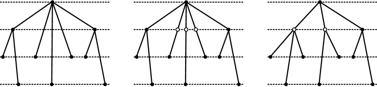
Figure 1: The regrouping process: left the original tree (partially represented), center the tree with added vertices, right the tree with regrouped branches.

Below depth $1$, the tree is unchanged and there is therefore a natural identification of $X$ with the level $0$ in $T^{1}$, and the distance induced by $T^{1}$ is no larger than the original one (it can be much smaller for some pair of points, and this is why we will only obtain a co-Lipschitz map). Another way to put it is that there is a bijective and $1$-Lipschitz map $f^{1}:X\to X^{1}$ where $X^{1}$ is the level $0$ of $T^{1}$. Moreover $\mu^{1}:=f^{1}_{\#}\mu$ is a probability measure on $X^{1}$ satisfying both

$$\mu^{1}(X^{1}_{v})\leq C(\mathop{\mathrm{missing}}{diam}\nolimits X^{1}_{v})^{s^{\prime}}=C\cdot q^{-ns^{\prime}}$$

when $v$ has height $q^{-n}$ with $n>1$ and

$$\frac{1}{2}Cq^{-s^{\prime}}\leq\mu^{1}(X^{1}_{v})\leq\frac{3}{2}Cq^{-s^{\prime}}$$

when $v$ is a child of the root (i.e., has height $q^{-1}$).

We can then inductively construct a sequence $T^{2},T^{3},\dots,T^{k},\dots$ of SRT by performing the same regrouping process at depth $k$ (i.e., the vertices of height $q^{-(k-1)}$ play the role played above by $o$). First this construction ensures that in $T^{k}$, a child $v$ of any vertex $v^{*}$ of height $h^{k}(v^{*})=q^{-n}$ for any $n<k$ must have height $h^{k}(v)=q^{-(n+1)}$. We also get a system of bijective $1$-Lipschitz maps $f^{k}:X^{k-1}\to X^{k}$ where $X^{k}$ is the ultrametric space defined by $T^{k}$, and probability measures $\mu^{k}$ that satisfy

$$\mu^{k}(X^{k}_{v})\leq C(\mathop{\mathrm{missing}}{diam}\nolimits X^{k}_{v})^{s^{\prime}}=C\cdot q^{-ns^{\prime}}$$

when $v$ has height $q^{-n}$ with $n>k$ and

$$\frac{1}{2}Cq^{-ns^{\prime}}\leq\mu^{k}(X^{k}_{v})\leq\frac{3}{2}Cq^{-ns^{\prime}}$$

when $v$ has height $q^{-n}$ with $n\leq k$.

Since $T_{k}$ and $T_{k+1}$ are isomorphic up to depth $k$, we get a limit SRT $T^{\infty}$, defining an ultrametric space $X^{\infty}$ and there is a $1$-Lipschitz map $f:X\to X^{\infty}$ obtained by composing all $f^{k}$. This map needs not be bijective, because some distances may have been reduced to zero in the process, collapsing some points together; but it certainly is onto.

Moreover, the probability measure $f^{\infty}_{\#}\mu=\mu^{\infty}$ satisfies

$$\frac{1}{2}Cq^{-ns^{\prime}}\leq\mu^{\infty}(X^{\infty}_{v})\leq\frac{3}{2}Cq^{-ns^{\prime}}$$

whenever $v$ has depth $n$. This ensures that any vertex in $T^{\infty}$ (except possibly the root) has at least

$$\frac{\frac{1}{2}Cq^{-ns^{\prime}}}{\frac{3}{2}Cq^{-(n+1)s^{\prime}}}=\frac{q^{s^{\prime}}}{3}=k$$

children. In particular, $T^{\infty}$ has a subtree isomorphic to the SRT of $Y$, so that there is an isometric embedding $g:Y\to X^{\infty}$.

Composing $g$ with a right inverse of $f^{\infty}$ (which exists at worst in the measurable category in virtue of a classical selection theorem), we get a co-Lipschitz map $Y\to X$, which proves Theorem 1.3 (recall that our choice of parameter ensures $\dim Y\geq s$).

5 Size of Wasserstein spaces

5.1 The case of regular ultrametric spaces

In the previous Section, we saw that ultrametric spaces contain co-Lipschitz images of large regular ultrametric spaces. To prove Theorem 1.2 we therefore have mainly left to estimate the size of Wasserstein spaces of regular ultrametric spaces.

.

Given any regular compact ultrametric space $Y=Y(k,q)$ and any $p\geq 1$, we have

$$\mathop{\mathrm{missing}}{crit}\nolimits_{\mathscr{P}}\mathop{\mathscr{W}}\nolimits_{p}(Y)=\log_{q}(k)=\dim Y.$$

Proof.

Since the upper Minkowski dimension of $Y$ is equal to its Hausdorff dimension, the upper bound $\mathop{\mathrm{missing}}{crit}\nolimits_{\mathscr{P}}\mathop{\mathscr{W}}\nolimits_{p}(Y)\leq\dim Y$ is given by Proposition 7.4 in [Klo12]. To prove the lower bound, we shall embed large Banach cubes in $\mathop{\mathscr{W}}\nolimits_{p}(Y)$. Fix any positive $\varepsilon$.

Label as usual the vertices of the SRT for $Y$ (i.e, its balls) by the finite words on the letters $\{1,\dots,k\}$. A vertex $v=i_{1}i_{2}\dots i_{n}$ is said to have depth $n$, has height $\frac{1}{2}q^{-n}$, and there are $k^{n}$ of them. Let $V^{\prime}$ be the set of vertices $v=i_{1}\dots i_{n}$ such that $i_{n}<k$, and define a map $\varphi:[0,1]^{V^{\prime}}\to\mathop{\mathscr{missing}}{P}\nolimits(Y)$ as follows. The measure $\mu=\varphi((a_{v})_{v\in V^{\prime}})$ is determined by the weight it gives to the balls $Y_{v}$ ($v\in V$) of $Y$, which we define recursively on the depth to be:

• $\mu(Y)=1$,

• $\displaystyle\mu(Y_{v})=\mu(Y_{v^{*}})\cdot\frac{1+\varepsilon a_{v}}{k}$ when $v\in V^{\prime}$,

• $\displaystyle\mu(Y_{v})=\mu(Y_{v^{*}})-\sum_{w^{*}=v^{*},w\neq v}\mu(Y_{w})$ when $v=i_{1}\dots i_{n-1}k$.

In other words, at each level we split mass almost equally between the children, allowing it to be slightly larger than average for the $k-1$ first children and consequently slightly smaller for the last one.

The first and second items are mandatory to get a well defined probability measure, taking $\varepsilon$ small enough ensures that all these values are positive, and this construction ensures that

$$\mu(Y_{v})\geq\left(\frac{1-(k-1)\varepsilon}{k}\right)^{n}$$

whenever $v$ has depth $n$.

From (2) in Section 3, we deduce that for all $a=(a_{v}),b=(b_{v})\in[0,1]^{V^{\prime}}$:

$$\mathop{\mathrm{W}}\nolimits_{p}(\varphi(a),\varphi(b))^{p}\geq C\sum_{v\in V^{\prime}}q^{-pn}\left(\frac{1-(k-1)\varepsilon}{k}\right)^{n}|a_{v}-b_{v}|$$

where the positive constant $C$ depends on $q,k,p,\varepsilon$ and $n=n(v)$ is the depth.

Since there are $(k-1)k^{n-1}$ vertices of depth $n$ in $V^{\prime}$, if we identify the vertices with the positive integers in a way that makes the depth function $n$ non-decreasing, we can identify the sequence

$$\left(q^{-p}\frac{1-(k-1)\varepsilon}{k}\right)^{n}(v)$$

where $v$ runs over the vertices with an integer-indexed sequence $(a_{m})$ where

$$a_{m}=\Theta\left(q^{-p}\frac{1-(k-1)\varepsilon}{k}\right)^{\log_{k}m}=\Theta\left(m^{\log_{k}(\frac{q^{-p}}{k}-O(\varepsilon))}\right).$$

It follows that there is a co-Lipschitz map from $\mathop{\mathrm{missing}}{BC}\nolimits((m^{-\alpha})_{m})$ to $(\mathop{\mathscr{missing}}{P}\nolimits(Y),\mathop{\mathrm{W}}\nolimits_{p}^{p})$ with

$$\alpha=1+p\frac{\ln q}{\ln k}-O(\varepsilon)=1+\frac{p}{\dim Y}-O(\varepsilon).$$

As a consequence,

$$\mathop{\mathrm{missing}}{crit}\nolimits_{\mathscr{P}}(\mathop{\mathscr{missing}}{P}\nolimits(Y),\mathop{\mathrm{W}}\nolimits_{p}^{p})\geq\mathop{\mathrm{missing}}{crit}\nolimits_{\mathscr{P}}\mathop{\mathrm{missing}}{BC}\nolimits((n^{-\alpha}))=\frac{1}{\alpha-1}$$

and letting $\varepsilon$ go to $0$, we have $\mathop{\mathrm{missing}}{crit}\nolimits_{\mathscr{P}}(\mathop{\mathscr{missing}}{P}\nolimits(Y),\mathop{\mathrm{W}}\nolimits_{p}^{p})\geq\dim Y/p$ from which $\mathop{\mathrm{missing}}{crit}\nolimits_{\mathscr{P}}\mathop{\mathscr{W}}\nolimits_{p}(Y)\geq\dim Y$ follows. ∎

5.2 The main Theorem and corollaries

Now the proof of Theorem 1.2 is easy: we are given a compact metric space $X$, and we want to prove

$$\mathop{\mathrm{missing}}{crit}\nolimits_{\mathscr{P}}\mathop{\mathscr{W}}\nolimits_{p}(Y)\geq\dim X.$$

If $\dim X=0$ there is nothing to prove; assume otherwise and choose arbitrary $s<s^{\prime}<\dim X$. There is a bi-Lipschitz embedding of an ultrametric space $X^{\prime}$ into $X$ with $\dim X^{\prime}\geq s^{\prime}$ (by the Mendel-Naor ultrametric skeleton theorem) and there is a co-Lipschitz embedding of a regular ultrametric space $Y$ into $X^{\prime}$ with $\dim Y\geq s$ (by Theorem 1.3). Composing these embeddings and applying the resulting map to measures, we get a co-Lipschitz embedding $\mathop{\mathscr{W}}\nolimits_{p}(Y)\hookrightarrow\mathop{\mathscr{W}}\nolimits_{p}(X)$. This implies that

$$\mathop{\mathrm{missing}}{crit}\nolimits_{\mathscr{P}}\mathop{\mathscr{W}}\nolimits_{p}(X)\geq\mathop{\mathrm{missing}}{crit}\nolimits_{\mathscr{P}}\mathop{\mathscr{W}}\nolimits_{p}(Y)=\dim Y\geq s$$

and since $s<\dim X$ is arbitrary, we finally get $\mathop{\mathrm{missing}}{crit}\nolimits_{\mathscr{P}}\mathop{\mathscr{W}}\nolimits_{p}(X)\geq\dim X$.

The two corollaries then follow directly. Assume $X$ is a compact space; we just saw that $\mathop{\mathrm{missing}}{crit}\nolimits_{\mathscr{P}}\mathop{\mathscr{W}}\nolimits_{p}(X)\geq\dim X$, and we proved in [Klo12] that $\mathop{\mathrm{missing}}{crit}\nolimits_{\mathscr{P}}\mathop{\mathscr{W}}\nolimits_{p}(X)\leq\mathop{\operatorname{\overline{M}-dim}}\nolimits X$. If $\dim X=\mathop{\operatorname{\overline{M}-dim}}\nolimits X=d$, then we get $\mathop{\mathrm{missing}}{crit}\nolimits_{\mathscr{P}}\mathop{\mathscr{W}}\nolimits_{p}(X)=d$. If $\dim X>\mathop{\operatorname{\overline{M}-dim}}\nolimits X^{\prime}$, we get $\mathop{\mathrm{missing}}{crit}\nolimits_{\mathscr{P}}\mathop{\mathscr{W}}\nolimits_{p}(X)>\mathop{\mathrm{missing}}{crit}\nolimits_{\mathscr{P}}\mathop{\mathscr{W}}\nolimits_{p^{\prime}}(X^{\prime})$, and there cannot be any bi-Lipschitz (or even co-Lipschitz) map from the first Wasserstein space to the second one.

6 An alternative proof of Theorem 1.2

We can prove Theorem 1.2 without the intermediate of ultrametric spaces, by using instead a sequence of points with controlled distances.

.

If $X$ is a metric space of Hausdorff dimension $d$, then for all $d^{\prime}<d$ there exist a constant $C$ and a sequence of points $(q_{i})$ in $X$ such that for all $i<j$ it holds $d(q_{i},q_{j})\geq Ci^{-1/d^{\prime}}$.

Proof.

This is a consequence of Frostman’s Lemma. Given $d^{\prime\prime}\in(d^{\prime},d)$, there is a probability measure $\mu$ on $X$ such that $\mu(B(p,r))\leq C_{1}r^{d^{\prime\prime}}$ for some constant $C_{1}$ and all $p$ in its support. For all integer $i>0$, let $a_{i}=C_{2}i^{-(1+\varepsilon)}$ where $\varepsilon$ will be chosen small afterward, and $C_{2}$ is such that $\sum a_{i}=1$. Let $r_{i}=(a_{i}/C_{1})^{\frac{1}{d^{\prime\prime}}}$

Choose $q_{1}\in\mathop{\mathrm{supp}}\nolimits\mu$ arbitrarily; then $\mu(B(q_{1},r_{1}))\leq a_{1}<1$ so there is a $q_{2}$ outside $B(q_{1},r_{1})$. We construct recursively $B_{j}=B(q_{j},r_{j})$ and $q_{j}$ outside $\cup_{i<j}B_{i}$. this is possible because

$$\mu(B_{1}\cup\dots B_{j-1})\leq a_{1}+\dots a_{j-1}<1=\mu(X).$$

We then get that $d(q_{i},q_{j})$ is at least $r_{i}=Ci^{-\frac{1+\varepsilon}{d^{\prime\prime}}}$ and we only have left to choose $\varepsilon$ and $d^{\prime\prime}$ appropriately. ∎

Let $d^{\prime}<d$ be fixed, and $(q_{i})$ be a sequence of points of $X$ as given by the lemma. Consider the map

$$\Phi:[0,1]^{\mathbb{N}} \to\mathop{\mathscr{W}}\nolimits_{p}(X)$$

$$\bar{x}=(x_{1},\dots) \mapsto\sum_{i\geq 1}b_{i}x_{i}\delta_{q_{i+1}}+(1-\sum_{i\geq 1}b_{i}x_{i})\delta_{q_{1}}$$

where $b_{i}=C_{3}i^{-(1+\varepsilon)}$ with $\varepsilon$ arbitrarily small and $C_{3}=C_{3}(\varepsilon)$ is such that $\sum b_{i}\leq 1$.

Then we easily get the lower estimate

$$\mathop{\mathrm{W}}\nolimits_{p}^{p}(\Phi(\bar{x}),\Phi(\bar{y}))\geq\sum_{i\geq 1}b_{i}|x_{i}-y_{i}|\cdot C^{p}(i+1)^{-\frac{p}{d^{\prime}}}.$$

Indeed, any transport plan from $\Phi(\bar{x})$ to $\Phi(\bar{y})$ must move a mass at least $b_{i}|x_{i}-y_{i}|$ from or to the point $q_{i}$, thus this amount is moved by a distance at least $C(i+1)^{-\frac{1}{d^{\prime}}}$.

We can identify $[0,1]^{\mathbb{N}}$ with any $\mathop{\mathrm{missing}}{BC}\nolimits((n^{-\alpha}))$ by suitable dilation along each coordinate. Taking $\alpha=p/d^{\prime}+1+\varepsilon$, we get that

$$W_{p}^{p}(\Phi(\bar{x}),\Phi(\bar{y}))\geq C_{4}d(\bar{x},\bar{y})$$

where the distance on the right-hand side is obtained from $\mathop{\mathrm{missing}}{BC}\nolimits((n^{-\alpha}))$ by the identification.

From (1) page 1 we know that there is a probability measure $\mu$ on $\mathop{\mathrm{missing}}{BC}\nolimits((n^{-\alpha}))$ such that

$$\log\mu(B(\bar{x},r)\leq C_{5}r^{\frac{-1}{\alpha-1}}=C_{5}r^{\frac{-1}{p/d^{\prime}+\varepsilon}}$$

(this is Frostman’s Lemma, or rather what one proves to bound from below the critical parameter of the Banach cube).

Consider the pushed forward measure $\Phi_{\#}\mu$ on $\mathop{\mathscr{W}}\nolimits_{p}(X)$: for all $\bar{x}\in\mathop{\mathrm{missing}}{BC}\nolimits((n^{-\alpha}))$ we have

$$\log\Phi_{\#}\mu(B(\Phi(\bar{x}),r)) \leq\log\mu(B(\bar{x},r^{p}/C_{4}))$$

$$\leq C_{6}r^{-\frac{p}{p/d^{\prime}+\varepsilon}}$$

This shows that the image of $\Phi$, and therefore $\mathop{\mathscr{W}}\nolimits_{p}(X)$ as well, has $\mathscr{P}$-critical parameter at least

$$\frac{p}{\frac{p}{d^{\prime}}+\varepsilon}$$

for all $\varepsilon>0$ and all $d^{\prime}<d$. Letting $\varepsilon\to 0$ and $d^{\prime}\to d$, we get that $\mathop{\mathrm{missing}}{crit}\nolimits_{\mathcal{P}}\mathop{\mathscr{W}}\nolimits_{p}(X)\geq d$, as desired.

.

One could think that Lemma 6 should hold under a condition on Minkowski dimension rather than Hausdorff dimension. In next section an example is given showing that this is far from being true.

7 Concluding examples

7.1 A large space with small parts

To show that the Hausdorff dimension hypothesis in Lemma 6 cannot easily be relaxed, let us prove the following.

.

There is a compact metric space $X$ with lower Minkowski dimension equal to $1$, all of whose proper closed subset have vanishing lower Minkowski dimension.

This set $X$ is therefore “large” in the sense of lower Minkowski dimension, but its closed parts are all “small” in the same sense. The example we shall construct has the additional properties to have a Minkowski dimension (lower and upper dimension match) and to be ultrametric. Before proving the Proposition, let us see how it relates to Lemma 6.

.

There is a compact metric space $X$ with positive lower Minkowski dimension $d$, but such that for no $d^{\prime}>0$ and no $C$ does it exists a sequence $(q_{i})$ in $X$ with $d(q_{i},q_{j})\geq Ci^{-1/d^{\prime}}$ for all $i<j$.

Proof.

If a space $Y$ contains a sequence $(q_{i})$ with $d(q_{i},q_{j})\geq Ci^{-1/d^{\prime}}$ for all $i<j$, then it has lower Minkowski dimension at least $d^{\prime}$, as for any $\varepsilon$ one needs at least $N=\lfloor(C/\varepsilon)^{d^{\prime}}\rfloor$ sets of diameter $\varepsilon$ to cover the the $N$ first points in the sequence.

Now, if the space $X$ given by Proposition 7.1 had such a sequence, its proper closed subset $Y=X\setminus B(q_{1},C)$ would contain the sequence $(q_{i})_{i>1}$ and therefore have lower Minkowski dimension at least $d^{\prime}$, a contradiction. ∎

Proof of Proposition 7.1.

We construct $X$ as an ultrametric space. Its SRT $T$ is given in terms of two sequences $(a_{n})$, $(h_{n})$ to be chosen suitably afterward. Its vertices are numbered $1,2,\dots$ by a breadth-first search, and the vertex $n$ has $a_{n}$ children. In other words, $1$ is the root, $2,\dots,1+a_{1}$ are the depth-$1$ vertices, $a_{1}+2,a_{1}+3,\dots,a_{1}+a_{2}+1$ are the children of $2$, and so on. We assume $a_{n}>1$ for all $n$, so that the SRT has no leaf and $X$ has the topology of a Cantor set. Then $h_{n}$, assumed to be decreasing, is the height of $n$.

Now, let $A_{n}=a_{1}+a_{2}+\dots+a_{n}-n+1$ be the number of branches of $T$ at height slightly below $h_{n}$. We set $a_{1}=2$, $a_{n+1}=A_{n}+1$ and $h_{1}=1$, $h_{n+1}=1/A_{n}$. In that way, $A_{n}=2^{n}$ and $h_{n}=2^{-n+1}$.

For any $\varepsilon$, let $n$ be such that $2^{-n+1}>\varepsilon\geqslant 2^{-n}$: one needs $2^{n}$ balls of radius $\varepsilon$ to cover $X$, and $2^{n}$ is between $1/\varepsilon$ and $2/\varepsilon$. Therefore, $X$ has Minkowski dimension $1$.

To prove that proper closed subset of $X$ have vanishing lower Minkowski dimension, we are reduced to consider $X\setminus B$ where $B$ is some ball, the set of descendants of vertex $i$ say. Let $k$ be a descendant of $i$: it has $A_{k-1}+1=2^{k-1}+1$ children, numbered from $n=k+1+2^{k-1}$ to $m=k+1+2^{k}$. Then $X\setminus B$ can be covered by less than $A_{n}$ balls of radius $\varepsilon=2^{-m}$. Since for large $k$, $A_{n}$ has the order of $\varepsilon^{-1/2}$, $X\setminus B$ has lower Minkowski dimension at most $1/2$.

But if $k$ is taken large enough, it has arbitrarily many successive siblings $k+1,k+2,\dots,k+N$ all of which are descendants of $i$. Then we can cover $X\setminus B$ by $A_{n}$ balls of radius $\varepsilon=2^{-M}$ with

$$M =n+A_{k-1}+1+A_{k}+1+\dots+A_{k+N}+1$$

$$\geq 2^{k-1}+2^{k-1}+2^{k}+2^{k+1}\dots+2^{k+n-1}$$

$$\geq 2^{k+N}-2^{k}=2^{k-1}(2^{N+1}-2)$$

For any $d>0$ and large enough $k$, we get that $A_{n}$ is far less than $\varepsilon^{-d}$. Therefore, the lower Minkowski dimension of $X\setminus B$ is zero. ∎

7.2 A small space with large Wasserstein space

Last, we prove Proposition 1.2. The example is constructed to have infinite Minkowski dimension (the number of branches above height $\varepsilon$ in its SRT grows very fast when $\varepsilon\to 0$) but small “complexity” (its SRT has countably many ends).

Let $T$ be the SRT such that the root has two children: a leaf $w_{1}$ (thus $h(w_{1})=0$), and $v_{2}$ which has two children: a leaf $w_{2}$, and $v_{3}$ which has two children and so on; and such that $h(o)=1$ and $h(v_{n})=(1+\ln n)^{-1}$. The ultrametric space $X$ defined by $T$ is a sequence $\{w_{1},w_{2},\dots\}$ together with an accumulation point $w_{\infty}$, and $d(w_{i},w_{j})=(1+\ln i)^{-1}$ when $1\leq i<j\leq\infty$.

For any $p>1$ and any $\mu,\nu\in\mathop{\mathscr{missing}}{P}\nolimits(X)$, formula (2) shows that

$$\mathop{\mathrm{W}}\nolimits_{p}(\mu,\nu)^{p}\geq\sum_{n\geq 1}\frac{1}{(1+\ln n)^{p}}|\mu(\{w_{n}\})-\nu(\{w_{n}\})|.$$

Fix any $\varepsilon>0$, and let $(b_{n})$ be the sequence of sum $1$ such that $b_{n}=Cn^{-(1+\varepsilon)}$ for some $C$ and all $n$. The map from $[0,1]^{\mathbb{N}}$ that sends $(m_{n})$ to the measure $\mu$ such that $\mu(\{w_{n}\})=m_{n}b_{n}$ is therefore co-Lipschitz from $\mathop{\mathrm{missing}}{BC}\nolimits((c_{n}))$ to $(\mathop{\mathscr{missing}}{P}\nolimits(X),\mathop{\mathrm{W}}\nolimits_{p}^{p})$ with

$$a_{n}=\frac{b_{n}}{(1+\ln n)^{p}}=\Theta\left(\frac{1}{n^{1+\varepsilon}(1+\ln n)^{p}}\right)=\Omega\left(\frac{1}{n^{1+2\varepsilon}}\right).$$

In particular, one can restrict this map to a co-Lipschitz map with domain $\mathop{\mathrm{missing}}{BC}\nolimits((n^{-(1+2\varepsilon)}))$ whose critical parameter is $1/2\varepsilon$. It follows that $\mathop{\mathrm{missing}}{crit}\nolimits_{\mathscr{P}}\mathop{\mathscr{W}}\nolimits_{p}(X)\geq\frac{p}{2\varepsilon}$, and this holds for all $\varepsilon>0$.

In conclusion, $X$ is a countable ultrametric space whose Wasserstein space has infinite power-exponential critical parameter, as claimed.

It seems plausible that (maybe at least for ultrametric spaces) the critical parameter of $\mathop{\mathscr{W}}\nolimits_{p}(X)$ is bounded below by the (lower or upper?) Minkowski dimension of $X$. The strongest conjecture would be that $\mathop{\mathrm{missing}}{crit}\nolimits_{\mathscr{P}}\mathop{\mathscr{W}}\nolimits_{p}(X)=\mathop{\operatorname{\overline{M}-dim}}\nolimits X$ for all compact metric space $X$. However we do not know how to transform an ultrametric space into one where explicit computations are possible without loosing too much of its Minkowski dimension, and general ultrametric spaces seem difficult to handle in wide generality. Moreover, we do not know whether there is an Ultrametric Skeleton Theorem with respect to Minkowski dimension (see Question 1.11 in [MN13b]).

References

- [BK12] J. Bertrand et B. R. Kloeckner – “A geometric study of Wasserstein spaces: Hadamard spaces”, J. Top. Ana. 4 (2012), no. 4, p. 515–542, arXiv:1010.0590.
- [GNS00] R. I. Grigorchuk, V. V. Nekrashevich et V. I. Sushchanskiĭ – “Automata, dynamical systems, and groups”, Tr. Mat. Inst. Steklova 231 (2000), no. Din. Sist., Avtom. i Beskon. Gruppy, p. 134–214.
- [Klo10] B. Kloeckner – “A geometric study of Wasserstein spaces: Euclidean spaces”, Ann. Sc. Norm. Super. Pisa Cl. Sci. (5) 9 (2010), no. 2, p. 297–323, arXiv:0804.3505.
- [Klo12] B. Kloeckner – “A generalization of Hausdorff dimension applied to Hilbert cubes and Wasserstein spaces”, J. Top. Ana. 4 (2012), no. 2, p. 203–235, arXiv:1105.0360.
- [Mat95] P. Mattila – Geometry of sets and measures in Euclidean spaces, Cambridge Studies in Advanced Mathematics, vol. 44, Cambridge University Press, Cambridge, 1995, Fractals and rectifiability.
- [McC97] R. J. McCann – “A convexity principle for interacting gases”, Adv. Math. 128 (1997), no. 1, p. 153–179.
- [MN13a] M. Mendel et A. Naor – “Ultrametric skeletons”, Proc. Natl. Acad. Sci. USA (2013), to appear.
- [MN13b] — , “Ultrametric subsets with large Hausdorff dimension”, Invent. Math. 192 (2013), no. 1, p. 1–54.
- [Nao12] A. Naor – “An introduction to the Ribe program”, Jpn. J. Math. 7 (2012), no. 2, p. 167–233.
- [Vil09] C. Villani – Optimal transport, old and new, Grundlehren der Mathematischen Wissenschaften, vol. 338, Springer-Verlag, 2009.