Some approximations in Model Checking and Testing

Abstract

Model checking and testing are two areas with a similar goal: to verify that a system satisfies a property. They start with different hypothesis on the systems and develop many techniques with different notions of approximation, when an exact verification may be computationally too hard. We present some notions of approximation with their logic and statistics backgrounds, which yield several techniques for model checking and testing: Bounded Model Checking, Approximate Model Checking, Approximate Black-Box Checking, Approximate Model-based Testing and Approximate Probabilistic Model Checking. All these methods guarantee some quality and efficiency of the verification.

Keywords: Approximation, verification, model checking, testing

1 Introduction

Model checking and Model-based testing are two methods for detecting faults in systems. Although similar in aims, these two approaches deal with very different entities. In model checking, a transition system (the model), which describes the system, is given and checked against some required or forbidden property. In testing, the executable system, called the Implementation Under Test (IUT) is given as a black box: one can only observe the behavior of the IUT on any chosen input, and then decide whether it is acceptable or not with respect to some description of its intended behavior.

However, in both cases the notions of models and properties play key roles: in model checking, the goal is to decide if a transition system satisfies or not some given property, often given in a temporal logic, by an automatic procedure that explores the model according to the property; in model-based testing, the description of the intended behavior is often given as a transition system, and the goal is to verify that the IUT conforms to this description. Since the IUT is a black box, the verification process consists in using the description model to construct a sequence of tests, such that if the IUT passes them, then it conforms to the description. This is done under the assumption that the IUT behaves as some unknown, maybe infinite, transition system.

An intermediate activity, black box checking combines model checking and testing as illustrated in the Figure 1 below, originally set up in [PVY99, Yan04]. In this approach, the goal is to verify a property of a system, given as a black box.

We concentrate on general results on efficient methods which guarantee some approximation, using basic techniques from complexity theory, as some tradeoff between feasibility and weakened objectives is needed. For example, in model checking some abstractions are made on the transition system according to the property to be checked. In testing, some assumptions are made on the IUT, like an upper bound on the number of states, or the uniformity of behavior on some input domain. These assumptions express the gap between the success of a finite test campaign and conformance. These abstractions or assumptions are specific to a given situation and generally do not fully guarantee the correctness.

Figure 1: Model checking, black box checking and testing.

This paper presents different notions of approximation which may be used in the context of model checking and testing. Current methods such as bounded model checking and abstraction, and most testing methods use some notions of approximation but it is difficult to quantify their quality. In this framework, hard problems for some complexity measure may become easier when both randomization and approximation are used. Randomization alone, i.e. algorithms of the class $\mathsf{BPP}$ may not suffice to obtain efficient solutions, as $\mathsf{BPP}$ may be equal to $\mathsf{P}$. Approximate randomized algorithms trade approximation with efficiency, i.e. relax the correctness property in order to develop efficient methods which guarantee the quality of the approximation. This paper emphasizes the variety of possible approximations which may lead to efficient verification methods, in time polynomial or logarithmic in the size of the domain, or constant (independent of the size of the domain), and the connections between some of them.

Section 2 sets the framework for model checking and model-based testing. Section 3 introduces two kinds of approximations: approximate techniques for satisfiability, equivalence and counting problems, and randomized techniques for the approximate versions of satisfiability and equivalence problems. Abstraction as a method to approximate a model checking problem, Uniform generation and Counting, and Learning are introduced in section 3.1. Property testing, the basic approach to approximate decision and equivalence problems, as well as statistical learning are defined in Section 3.2. Section 4 describes the five different types of approximation that we review in this paper, based on the logic and statistics tools of Section 3 for model checking and testing:

1. Bounded Model Checking where the computation paths are bounded (Section 4.1),

2. Approximate Model Checking where we use two distinct approximations: the proportion of inputs which separate the model and the property, and some edit distance between a model and a property (Section 4.2),

3. Approximate Black Box Checking where one approximately learns a model (Section 4.3),

4. Approximate Model-based Testing where one finds tests which approximately satisfy some coverage criterium (Section 4.4),

5. Approximate Probabilistic Model Checking where one approximates the probabilities of satisfying formulas (Section 4.5).

The methods we describe guarantee some quality of approximation and a complexity which ranges from polynomial in the size of the model, polynomial in the size of the representation of the model, to constant time:

1. In bounded model checking, some upper bounds on the execution paths to witness some error are stated for some class of formulas. The method is polynomial in the size of the model.

2. In approximate model checking, the methods guarantee with high probability that we discover some errors. We use two criteria. In the first approach, if the density of errors is larger than $\varepsilon$, Monte Carlo methods find them with high probabilities in polynomial time. In the second approach, if the distance of the inputs to the property is larger than $\varepsilon$, an error will be found with high probability. The time complexity is constant, i.e. independent of the size of the model but dependent on $\varepsilon$.

3. In approximate black box checking, learning techniques construct a model which can be compared with a property. Some intermediate steps, such as model checking are exponential in the size of the model. These steps can be approximated using the previous approximate model checking and guarantee that the model is $\varepsilon$-close to the IUT after $N$ samples, using learning techniques which depend on $\varepsilon$.

4. In approximate model-based testing, a coverage criterium is satisfied with high probability which depends on the number of tests. The method is polynomial in the size of the representation.

5. In approximate probabilistic model checking, the estimated probabilities of satisfying formulas are close to the real ones. The method is polynomial in the size of a succinct representation.

The paper focuses on approximate and randomized algorithms in model checking and model-based testing. Some common techniques and methods are pointed out. Not surprisingly the use of model checking techniques for model-based test generation has been extensively studied. Although of primary interest, this subject is not treated in this paper.

We believe that this survey will encourage some cross-fertilization and new tools both for approximate and probabilistic model checking, and for randomized model-based testing.

2 Classical methods in model checking and testing

Let $P$ be a finite set of atomic propositions, and ${\cal P}(P)$ the power set of $P$. A Transition System, or a Kripke structure, is a structure $\mathcal{M}=(S,s_{0},R,L)$ where $S$ is a finite set of states, $s_{0}\in S$ is the initial state, $R\subseteq S\times S$ is the transition relation between states and $L:~{}~{}S\rightarrow{\cal P}(P)$ is the labelling function. This function assigns labels to states such that if $p\in P$ is an atomic proposition, then $\mathcal{M},s\models p$, i.e. $s$ satisfies $p$ if $p\in L(s)$. Unless otherwise stated, the size of $\mathcal{M}$ is $|S|$, the size of $S$.

A Labelled Transition System on a finite alphabet $I$ is a structure $\mathcal{L}=(S,s_{0},I,R,L)$ where $S,s_{0},L$ are as before and $R\subseteq S\times I\times S$. The transitions have labels in $I$. A run on a word $w\in I^{*}$ is a sequence of states $s_{0},s_{1},....,s_{n}$ such that $(s_{i},w_{i},s_{i+1})\in R$ for $i=0,...,n-1$.

A Finite State Machine (FSM) is a structure $\mathcal{T}=(S,s_{0},I,O,R)$ with input alphabet $I$ and output alphabet $O$ and $R\subseteq S\times I\times O\times S$. An output word $t\in O^{*}$ is produced by an input word $w\in I^{*}$ of the FSM if there is a run, also called a trace, on $w$, i.e. a sequence of states $s_{0},s_{1},...,s_{n}$ such that $(s_{i},w_{i},t_{i},s_{i+1})\in R$ for $i=0,...,n-1$. The input/output relation is the pair $(w,t)$ when $t$ is produced by $w$. An FSM is deterministic if there is a function $\delta$ such that $\delta(s_{i},w_{i})=(t_{i},s_{i+1})~{}{\rm iff}~{}(s_{i},w_{i},t_{i},s_{i+1})\in R$. There may be a label function $L$ on the states, in some cases.

Other important models are introduced later. An Extended Finite State Machine (EFSM), introduced in section 2.3.3, assigns variables and their values to states and is a succinct representation of a much larger FSM. Transitions assume guards and define updates on the variables. A Büchi automaton, introduced in section 2.1.1, generalizes classical automata, i.e. FSM with no output but with accepting states, to infinite words. In order to consider probabilistic systems, we introduce Probabilistic Transition Systems and Concurrent Probabilistic Systems in section 2.2.

2.1 Model checking

Consider a transition system $\mathcal{M}=(S,s_{0},R,L)$ and a temporal property expressed by a formula $\psi$ of Linear Temporal Logic (LTL) or Computation Tree Logic (CTL and CTL^∗). The Model Checking problem is to decide whether $\mathcal{M}\models\psi$, i.e. if the system $\mathcal{M}$ satisfies the property defined by $\psi$, and to give a counterexample if the answer is negative.

In linear temporal logic LTL, formulas are composed from the set of atomic propositions using the boolean connectives and the main temporal operators $\mathbf{X}$ (next time) and $\mathbf{U}$ (until). In order to analyze the sequential behavior of a transition system $\mathcal{M}$, LTL formulas are interpreted over runs or execution paths of the transition system ${\cal M}$. A path $\sigma$ is an infinite sequence of states $(s_{0},s_{1},\dots,s_{i},\dots)$ such that $(s_{i},s_{i+1})\in R$ for all $i\geq 0$. We note $\sigma^{i}$ the path $(s_{i},s_{i+1},\dots)$. The interpretation of LTL formulas are defined by:

• if $p\in P$ then $\mathcal{M},\sigma\models p$ iff $p\in L(s_{0})$,

• $\mathcal{M},\sigma\models\neg\psi$ iff $\mathcal{M},\sigma\not\models\psi$,

• $\mathcal{M},\sigma\models\varphi\wedge\psi$ iff $\mathcal{M},\sigma\models\varphi$ and $\mathcal{M},\sigma\models\psi$,

• $\mathcal{M},\sigma\models\varphi\vee\psi$ iff $\mathcal{M},\sigma\models\varphi$ or $\mathcal{M},\sigma\models\psi$,

• $\mathcal{M},\sigma\models\mathbf{X}\psi$ iff $\mathcal{M},\sigma^{1}\models\psi$,

• $\mathcal{M},\sigma\models\varphi\mathbf{U}\psi$ iff there exists $i\geq 0$ such that $\mathcal{M},\sigma^{i}\models\psi$ and for each $0\leq j<i$, $\mathcal{M},\sigma^{j}\models\varphi$,

The usual auxiliary operators $\mathbf{F}$ (eventually) and $\mathbf{G}$ (globally) can also be defined: $true\equiv p\vee\neg p$ for some arbitrary $p\in P$, $\mathbf{F}\psi\equiv true\mathbf{U}\psi$ and $\mathbf{G}\psi\equiv\neg\mathbf{F}\neg\psi$.

In Computation Tree Logic CTL^∗, general formulas combine states and paths formulas.

1. A state formula is either

   • $p$ if $p$ is an atomic proposition, or

   • $\neg F$, $F\wedge G$ or $F\vee G$ where $F$ and $G$ are state formulas, or

   • $\exists\varphi$ or $\forall\varphi$ where $\varphi$ is a path formula.

2. A path formula is either

   • a state formula, or

   • $\neg\varphi$, $\varphi\wedge\psi$, $\varphi\vee\psi$, $\mathbf{X}\varphi$ or $\varphi\mathbf{U}\psi$ where $\varphi$ and $\psi$ are path formulas.

State formulas are interpreted on states of the transition system. The meaning of path quantifiers is defined by: given $\mathcal{M}$ and $s\in S$, we say that $\mathcal{M},s\models\exists\psi$ (resp. $\mathcal{M},s\models\forall\psi$) if there exists a path $\pi$ starting in $s$ which satisfies $\psi$ (resp. all paths $\pi$ starting in $s$ satisfy $\psi)$.

In CTL, each of the temporal operators $\mathbf{X}$ and $\mathbf{U}$ must be immediately preceded by a path quantifier. LTL can be also considered as the fragment of CTL^∗ formulas of the form $\forall\varphi$ where $\varphi$ is a path formula in which the only state subformulas are atomic propositions . It can be shown that the three temporal logics CTL^∗, CTL and LTL have different expressive powers.

The first model checking algorithms enumerated the reachable states of the system in order to check the correctness of a given specification expressed by an LTL or CTL formula. The time complexity of these algorithms was linear in the size of the model and of the formula for CTL, and linear in the size of the model and exponential in the size of the formula for LTL. The specification can usually be expressed by a formula of small size, so the complexity depends in a crucial way on the model’s size. Unfortunately, the representation of a protocol or of a program with boolean variables by a transition system illustrates the state explosion phenomenon: the number of states of the model is exponential in the number of variables. During the last twenty years, different techniques have been used to reduce the complexity of temporal logic model checking:

• automata theory and on-the-fly model construction,

• symbolic model checking and representation by ordered binary decision diagram (OBDD),

• symbolic model checking using propositional satisfiability (SAT) solvers.

2.1.1 Automata approach

This approach to verification is based on an intimate connection between linear temporal logic and automata theory for infinite words which was first explicitly discussed in [WVS83]. The basic idea is to associate with each linear temporal logic formula a finite automaton over infinite words that accepts exactly all the runs that satisfy the formula. This enables the reduction of decision problems such as satifiability and model checking to known automata-theoretic problems.

A nondeterministic Büchi automaton is a tuple $\mathcal{A}=(\Sigma,S,S_{0},\delta,F)$, where

• $\Sigma$ is a finite alphabet,

• $S$ is a finite set of states,

• $S_{0}\subseteq S$ is a set of initial states,

• $\delta:S\times\Sigma\longrightarrow 2^{S}$ is a transition function, and

• $F\subseteq S$ is a set of final states.

The automaton $\mathcal{A}$ is deterministic if $|\delta(s,a)|=1$ for all states $s\in S$, for all $a\in\Sigma$, and if $|S_{0}|=1$.

A run of $\mathcal{A}$ over a infinite word $w=a_{0}a_{1}\dots a_{i}\dots$ is a sequence $r=s_{0}s_{1}\dots s_{i}\dots$ where $s_{0}\in S_{0}$ and $s_{i+1}\in\delta(s_{i},a_{i})$ for all $i\geq 0$. The limit of a run $r=s_{0}s_{1}\dots s_{i}\dots$ is the set $lim(r)=\{s|s=s_{i}\mbox{ for infinitely many}~{}i\}$. A run $r$ is accepting if $lim(r)\cap F\neq\emptyset$. An infinite word $w$ is accepted by $\mathcal{A}$ if there is an accepting run of $\mathcal{A}$ over $w$. The language of $\mathcal{A}$, denoted by the regular language $L(\mathcal{A})$, is the set of infinite words accepted by $\mathcal{A}$. For any LTL formula $\varphi$, there exists a nondeterministic Büchi automaton $\mathcal{A}_{\varphi}$ such that the set of words satisfying $\varphi$ is the regular language $L(\mathcal{A})_{\varphi}$ and that can be constructed in time and space $O(|\varphi|.2^{|\varphi|})$. Moreover any transition system $\mathcal{M}$ can be viewed as a Büchi automaton $\mathcal{A}_{\mathcal{M}}$. Thus model checking can be reduced to the comparison of two infinite regular languages and to the emptiness problem for regular languages [VW86] : $\mathcal{M}\models\varphi$ iff $L(\mathcal{A}_{\mathcal{M}})\subseteq L(\mathcal{A}_{\varphi})$ iff $L(\mathcal{A}_{\mathcal{M}})\cap L(\mathcal{A}_{\neg\varphi})=\emptyset$ iff $L(\mathcal{A}_{\mathcal{M}}\times\mathcal{A}_{\neg\varphi})=\emptyset$.

In [VW86], the authors prove that LTL model checking can be decided in time $O(|\mathcal{M}|.2^{|\varphi|})$ and in space $O((log|\mathcal{M}|+|\varphi|)^{2})$, that is a refinement of the result in [SC85], which says that LTL model checking is PSPACE-complete. One can remark that a time upper bound that is linear in the size of the model and exponential in the size of the formula is considered as reasonable, since the specification is usually rather short. However, the main problem is the state explosion phenomenon due to the representation of a protocol or of a program to check, by a transition system.

The automata approach can be useful in practice for instance when the transition system is given as a product of small components $\mathcal{M}_{1},\dots,\mathcal{M}_{k}$. The model checking can be done without building the product automaton, using space $O((log|\mathcal{M}_{1}|+\dots+log|\mathcal{M}_{k}|)^{2})$ which is usually much less than the space needed to store the product automaton. In [GPVW95], the authors describe a tableau-based algorithm for obtaining an automaton from an LTL formula. Technically, the algorithm translates an LTL formula into a generalized Büchi automaton using a depth-first search. A simple transformation of this automaton yields a classical Büchi automaton for which the emptiness check can be done using a cycle detection scheme. The result is a verification algorithm in which both the transition model and the property automaton are constructed on-the-fly during a depth-first search that checks for emptiness. This algorithm is adopted in the model checker SPIN [Hol03].

2.1.2 OBDD approach

In symbolic model checking [BCM⁺92, McM93], the transition relation is coded symbolically as a boolean expression, rather than expicitly as the edges of a graph. A major breakthrough was achieved by the introduction of OBDD’s as a data structure for representing boolean expressions in the model checking procedure.

An ordered binary decision diagram (OBDD) is a data structure which can encode an arbitrary relation or boolean function on a finite domain. Given a linear order $<$ on the variables, it is a binary decision diagram, i.e.a directed acyclic graph with exactly one root, two sinks, labelled by the constants $1$ and $0$, such that each non-sink node is labelled by a variable $x_{i}$, and has two outgoing edges which are labelled by $1$ ($1$-edge) and $0$ ($0$-edge), respectively. The order, in which the variables appear on a path in the graph, is consistent with the variable order $<$, i.e. for each edge connecting a node labelled by $x_{i}$ to a node labelled by $x_{j}$, we have $x_{i}<x_{j}$.

Figure 2: Two OBDDs for a function $f:\{0,1\}^{3}\rightarrow\{0,1\}$.

Let us start with an OBDD representation of the relations $R$ of $\mathcal{M}$, the transition relation, and of each unary relation $P(x)$ describing states which satisfy the atomic propositions $p$. Given a CTL formula, one constructs by induction on its syntactic structure, an OBDD for the unary relation defining the states where it is true, and we can then decide if $\mathcal{M}\models\psi$. Figure 3 describes the construction of an OBDD for $R(x,y)\vee P(x)$ from an OBDD for $R(x,y)$ and an OBDD for $P(x)$. Each variable $x$ is decomposed in a sequence of boolean variables. In our example $x_{1},x_{2},x_{3}$ represent $x$ and similarly for $y$. The order of the variables is $x_{1},x_{2},x_{3},y_{1},y_{2},y_{3}$ in our example. Figure 3 presents a partial decision tree: the dotted line corresponds to $x_{i}=0$ and the standard line corresponds to $x_{i}=1$. The tree is partial to make it readable, and missing edges lead to $0$.

Figure 3: The construction of an OBDD for $R(x,y)\vee P(x)$.

The main drawback is that the OBDD can be exponentially large, even for simple formulas [Bry91]. The good choice of the order on the variables is important, as the size of the OBDD may vary exponentially if we change the order.

2.1.3 SAT approach

Symbolic model checking and symbolic reachability analysis can be reduced to the satisfiability problem for propositional formulas [BCCZ99a, ABE00a]. These reductions will be explained in the section 4.1: bounded and unbounded model checking. In the following, we recall the quest for efficient satisfiability solvers which has been the subject of an intensive research during the last twenty years.

Given a propositional formula which is presented in a Conjunctive Normal Form (CNF), the goal is to find a positive assignment of the formula. Recall that, a CNF is a conjunction of one or more clauses $C_{1}\wedge C_{2}\wedge C_{3}\wedge\ldots$, where each clause is a disjunction of one or more literals, $C_{1}=x_{1}\vee\bar{x}_{2}\vee\bar{x}_{5}\vee x_{7}$, $C_{2}=\bar{x}_{3}\vee x_{7}$, $C_{3}=\ldots$. A literal is either the positive or the negative occurrence of a propositional variable, for instance $x_{2}$ and $\bar{x}_{2}$ are the two literals for the variable $x_{2}$.

Due to the NP-completeness of SAT, it is unlikely that there exists any polynomial time solution. However, NP-completeness does not exclude the possibility of finding algorithms that are efficient enough for solving many interesting SAT instances. This was the motivation for the development of several successful algorithms [ZM02].

An original important algorithm for solving SAT, due to [DP60], is based on two simplification rules and one resolution rule. As this algorithm suffers from a memory explosion, [DLL62] proposed a modified version (DPLL) which performs a branching search with backtracking, in order to reduce the memory space required by the solver.

[MSS96] proposed an iterative version of DPLL, that is a branch and search algorithm. Most of the modern SAT solvers are designed in this manner and the main components of these algorithms are:

• a decision process to extend the current assignment to an unassigned variable; this decision is usually based on branching heuristics,

• a deduction process to propagate the logical consequences of an assignment to all clauses of the SAT formula; this step is called Boolean Constraint Propagation (BCP),

• a conflict analysis which may lead to the identification of one or more unsatisfied clauses, called conflicting clauses,

• a backtracking process to undo the current assignment and to try another one.

In a SAT solver, the BCP step is to propagate the consequences of the current variable assignment to the clauses. In CHAFF [MMZ⁺01], Moskewicz et al. proposed a BCP algorithm called two-literal watching with lazy update. Since the breakthrough of CHAFF, most effort in the design of efficient SAT solvers has been focused on efficient BCP, the heart of all modern SAT solvers.

An additional technique named Random restart was proposed to cope with the following phenomenon: two instances with the same clauses but different variable orders may require different times by a SAT solver. Experiments show that a random restart can increase the robustness of SAT solvers and this technique is applied in modern SAT solvers such as RSTART [PD07], TiniSAT [Hua07] and PicoSAT [Bie08]. This technique, for example the nested restart scheme used by PicoSAT, is inspired by the work of M. Luby et al. [LSZ93].

Another significant extension of DPLL is clause learning: when there is a conflict after some propagation, and there are still some branches to be searched, the cause of the conflict is analysed and added as a new clause before backtracking and continuing the search [BKS03]. Various learning schemes have been proposed [AS09] to derive the new clauses. Combined with non chronological backtracking and random restart these techniques are currently the basis of modern SAT-solvers, and the origin of the spectacular increase of their performance.

2.2 Verification of probabilistic systems

In this section, we consider systems modeled either as finite discrete time Markov chains or as Markov models enriched with a nondeterministic behavior. In the following, the former systems will be denoted by probabilistic sytems and the latter by concurrent probabilistic sytems. A Discrete Time Markov Chain (DTMC) is a pair $(S,M)$ where $S$ is a finite or countable set of states and $M:S\times S\rightarrow[0,1]$ is the stochastic matrix giving the transition probabilities, i.e. for all $s\in S$, $\sum_{t\in S}M(s,t)=1$. In the following, the set of states $S$ is finite.

Definition 1

A probabilistic transition system ($PTS$) is a structure $\mathcal{M}_{p}=(S,s_{0},M,L)$ given by a Discrete Time Markov chain $(S,M)$ with an initial state $s_{0}$ and a function $L:S\rightarrow\mathcal{P}(P)$ labeling each state with a set of atomic propositions in $P$.

A path $\sigma$ is a finite or infinite sequence of states $(s_{0},s_{1},\dots,s_{i},\dots)$ such that $P(s_{i},s_{i+1})$ $>0$ for all $i\geq 0$. We denote by $Path(s)$ the set of paths whose first state is $s$. For each structure ${\cal M}$ and state $s$, it is possible to define a probability measure $Prob$ on the set $Path(s)$. For any finite path $\pi=(s_{0},s_{1},\dots,s_{n})$, the measure is defined by:

$$Prob(\{\sigma~{}:~{}\sigma\mbox{ is a path with prefix }~{}\pi\})=\prod_{i=1}^{n}M(s_{i-1},s_{i})$$

This measure can be extended uniquely to the Borel family of sets generated by the sets $\{\sigma~{}:~{}\pi\mbox{ is a prefix of }\sigma\}$ where $\pi$ is a finite path. In [Var85], it is shown that for any $LTL$ formula $\psi$, probabilistic transition system ${\cal M}$ and state $s$, the set of paths $\{\sigma~{}:~{}{\sigma_{0}=s\mbox{ and }\cal M},\sigma\models\psi\}$ is measurable. We denote by $Prob[\psi]$ the measure of this set and by $Prob_{k}[\psi]$ the probability measure associated to the probabilistic space of execution paths of finite length $k$.

2.2.1 Qualitative verification

We say that a probabilistic transition sytem ${\cal M}_{p}$ satisfies the formula $\psi$ if $Prob[\psi]=1$, i.e. if almost all paths in ${\cal M}$, whose origin is the initial state, satisfy $\psi$. The first application of verification methods to probabilistic systems consisted in checking if temporal properties are satisfied with probability $1$ by a finite discrete time Markov chain or by a concurrent probabilistic sytem. [Var85] presented the first method to verify if a linear time temporal property is satisfied by almost all computations of a concurrent probabilistic system. However, this automata-theoretic method is doubly exponential in the size of the formula.

The complexity was later addressed in [CY95]. A new model checking method for probabilistic systems was introduced, whose complexity was polynomial in the size of the system and exponential in the size of the formula. For concurrent probabilistic systems they presented an automata-theoretic approach which improved on Vardi’s method by a single exponential in the size of the formula.

2.2.2 Quantitative verification

The [CY95] method allows to compute the probability that a probabilistic system satisfies some given linear time temporal formula.

Theorem 1

([CY95]) The satisfaction of a $LTL$ formula $\phi$ by a probabilistic transition sytem ${\cal M}_{p}$ can be decided in time linear in the size of ${\cal M}_{p}$ and exponential in the size of $\phi$, and in space polylogarithmic in the size of ${\cal M}_{p}$ and polynomial in the size of $\phi$. The probability $Prob[\phi]$ can be computed in time polynomial in size of ${\cal M}_{p}$ and exponential in size of $\phi$.

A temporal logic for the specification of quantitative properties, which refer to a bound of the probability of satisfaction of a formula, was given in [HJ94]. The authors introduced the logic PCTL, which is an extension of branching time temporal logic CTL with some probabilistic quantifiers. A model checking algorithm was also presented: the computation of probabilities for formulas involving probabilistic quantification is performed by solving a linear system of equations, the size of which is the model size.
A model checking method for concurrent probabilistic systems against PCTL and PCTL^∗ (the standard extension of PCTL) properties is given in [BdA95]. Probabilities are computed by solving an optimisation problem over system of linear inequalities, rather than linear equations as in [HJ94]. The algorithm for the verification of PCTL^∗ is obtained by a reduction to the PCTL model checking problem using a transformation of both the formula and the probabilistic concurrent system. Model checking of PCTL formulas is shown to be polynomial in the size of the system and linear in the size of the formula, while PCTL^∗ verification is polynomial in the size of the system and doubly exponential in the size of the formula.

In order to illustrate space complexity problems, we mention the main model checking tool for the verification of quantitative properties. The probabilistic model checker PRISM [dAKN⁺00, HKNP06] was designed by the Kwiatkowska’s team and allows to check PCTL formulas on probabilistic or concurrent probabilistic systems. This tool uses extensions of OBDDs called Multi-Terminal Binary Decision Diagrams (MTBDDs) to represent Markov transition matrices, and classical techniques for the resolution of linear systems. Numerous classical protocols represented as probabilistic or concurrent probabilistic systems have been successfully verified by PRISM. But experimental results are often limited by the exponential blow up of space needed to represent the transition matrices and to solve linear systems of equations or inequations. In this context, it is natural to ask the question: can probabilistic verification be efficiently approximated? We study in Section 4.5 some possible answers for probabilistic transition systems and linear time temporal logic.

2.3 Model-based testing

Given some executable implementation under test and some description of its expected behavior, the IUT is submitted to experiments based on the description. The goal is to (partially) check that the IUT is conforming to the description. As we explore links and similarities with model checking, we focus on descriptions defined in terms of finite and infinite state machines, transitions systems, and automata. The corresponding testing methods are called Model-based Testing.

Model-based testing has received a lot of attention and is now a well established discipline (see for instance [LY96, BT01, BJK⁺05]). Most approaches have focused on the deterministic derivation from a finite model of some so-called checking sequence, or of some complete set of test sequences, that ensure conformance of the IUT with respect to the model. However, in very large models, such approaches are not practicable and some selection strategy must be applied to obtain test sets of reasonable size. A popular selection criterion is the transition coverage. Other selection methods rely on the statement of some test purpose or on random choices among input sequences or traces.

2.3.1 Testing based on finite state machines

As in [LY96], we first consider testing methods based on deterministic FSMs: instead of $\mathcal{T}=(S,s_{0},I,O,R)$ where $R\subseteq S\times I\times O\times S$, we have $\mathcal{F}=(S,I,O,\delta,\lambda)$. where $\delta$ and $\lambda$ are functions from $S\times I$ into $S$, and from $S\times I$ into $O$, respectively. There is not always an initial state. Functions $\delta$ and $\lambda$ can be extended in a canonic way to sequences of inputs: $\delta^{*}$ is from $S\times I^{*}$ into $S^{*}$and $\lambda^{*}$ is from $S\times I^{*}$ into $O^{*}$.

The testing problem addressed in this subsection is: given a deterministic specification FSM $A$, and an IUT that is supposed to behave as some unknown deterministic FSM $B$, how to test that $B$ is equivalent to $A$ via inputs submitted to the IUT and outputs observed from the IUT? The specification FSM must be strongly connected, i.e., there is a path between every pair of states: this is necessary for designing test experiments that reach every specified state.

Equivalence of FSMs is defined as follows. Two states $s_{i}$ and $s_{j}$ are equivalent if and only if for every input sequence, the FSMs will produce the same output sequence, i.e., for every input sequence $\sigma$, $\lambda^{*}(s_{i},\sigma)=\lambda^{*}(s_{j},\sigma)$. $\mathcal{F}$ and $\mathcal{F}^{\prime}$ are equivalent if and only for every state in $\mathcal{F}$ there is a corresponding equivalent state in $\mathcal{F}^{\prime}$, and vice versa. When $\mathcal{F}$ and $\mathcal{F}^{\prime}$ have the same number of states, this notion is the same as isomorphism. Given an FSM, there are well-known polynomial algorithms for constructing a minimized (reduced) FSM equivalent to the given FSM, where there are no equivalent states. The reduced FSM is unique up to isomorphism. The specification FSM is supposed to be reduced before any testing method is used.

Any test method is based on some assumption on the IUT called testability hypotheses. An example of a non testable IUT would be a “demonic” one that would behave well during some test experiments and change its behavior afterwards. Examples of classical testability hypotheses, when the test is based on finite state machine descriptions, are:

• The IUT behaves as some (unknown) finite state machine.

• The implementation machine does not change during the experiments.

• It has the same input alphabet as the specification FSM.

• It has a known number of states greater or equal to the specification FSM.

This last and strong hypothesis is necessary to develop testing methods that reach a conclusion after a finite number of experiments. In the sequel, as most authors, we develop the case where the IUT has the same number of states as the specification FSM. Then we give some hints on the case where it is bigger.

A test experiment based on a FSM is modelled by the notion of checking sequence, i. e. a finite sequence of inputs that distinguishes by some output the specification FSM from any other FSM with at most the same number of states.

Definition 2

Let $A$ be a specification FSM with $n$ states and initial state $s_{0}$. A checking sequence for $A$ is an input sequence $\sigma_{check}$ such that for every FSM $B$ with initial state $s^{\prime}_{0}$, the same input alphabet, and at most $n$ states, that is not isomorphic to $A$, $\lambda^{*}_{B}(s^{\prime}_{0},\sigma_{check})\neq\lambda^{*}_{A}(s_{0},\sigma_{check})$.

The complexity of the construction of checking sequences depends on two important characteristics of the specification FSM: the existence of a reliable reset that makes it possible to start the test experiment from a known state, and the existence of a distinguishing sequence $\sigma$, which can identify the resulting state after an input sequence, i.e. such that for every pair of distinct states $s_{i}$, $s_{j}$, $\lambda^{*}(s_{i},\sigma)\neq\lambda^{*}(s_{j},\sigma)$.

A reliable reset is a specific input symbol that leads an FSM from any state to the same state: for every state $s$, $\delta(s,reset)=s_{r}$. For FSM without reliable reset, the so-called homing sequences are used to start the checking sequence. A homing sequence is an input sequence $\sigma_{h}$ such that, from any state, the output sequence produced by $\sigma_{h}$ determines uniquely the arrival state. For every pair of distinct states $s_{i},s_{j},\lambda^{*}(s_{i},\sigma_{h})=\lambda^{*}(s_{j},\sigma_{h})$ implies $\delta^{*}(s_{i},\sigma_{h})=\delta^{*}(s_{j},\sigma_{h})$. Every reduced FSM has an homing sequence of polynomial length, constructible in polynomial time.

The decision whether the behavior of the IUT is satisfactory, requires to observe the states of the IUT either before or after some action. As the IUT is a running black box system, the only means of observation is by submitting other inputs and collecting the resulting outputs. Such observations are generally destructive as they may change the observed state.

The existence of a distinguishing sequence makes the construction of a checking sequence easier: an example of a checking sequence for a FSM $A$ is a sequence of inputs resulting in a trace that traverses once every transition followed by this distinguishing sequence to detect for every transition both output errors and errors of arrival state.

Unfortunately deciding whether a given FSM has a distinguishing sequence is PSPACE-complete with respect to the size of the FSM (i.e. the number of states). However, it is polynomial for adaptative distinguishing sequences (i.e input trees where choices of the next input are guided by the outputs of the IUT), and it is possible to construct one of quadratic length. For several variants of these notions, see [LY96].

Let $p$ the size of the input alphabet. For an FSM with a reliable reset, there is a polynomial time algorithm, in $O(p.n^{3})$, for constructing a checking sequence of polynomial length, also in $O(p.n^{3})$ [Vas73, Cho78]. For an FSM with a distinguishing sequence there is a deterministic polynomial time algorithm to construct a checking sequence [Hen64, KHF90] of length polynomial in the length of the distinguishing sequence.

In other cases, checking sequences of polynomial length also exist, but finding them requires more involved techniques such as randomized algorithms. More precisely, a randomized algorithm can construct with high probability in polynomial time a checking sequence of length $O(p.n^{3}+p^{\prime}.n^{4}.\log n)$, with $p^{\prime}=min(p,n)$. The only known deterministic complexity of producing such sequences is exponential either in time or in the length of the checking sequence.

The above definitions and results generalize to the case where FSM $B$ has more states than FSM $A$. The complexity of generating checking sequences, and their lengths, are exponential in the number of extra states.

2.3.2 Non determinism

The concepts presented so far are suitable when both the specification FSM and the IUT are deterministic. Depending on the context and of the authors, a non deterministic specification FSM $A$ can have different meanings: it may be understood as describing a class of acceptable deterministic implementations or it can be understood as describing some non deterministic acceptable implementations. In both cases, the notion of equivalence of the specification FSM $A$ and of the implementation FSM $B$ is no more an adequate basis for testing. Depending of the authors, the required relation between a specification and an implementation is called the “satisfaction relation” ($B$ satisfies $A$) or the “conformance relation” ($B$ conforms to $A$). Generally it is not an equivalence, but a preorder (see [Tre92, GJ98, BT01] among many others).

A natural definition for this relation could be the so-called “trace inclusion” relation: any trace of the implementation must be a trace of the specification. Unfortunately, this definition accepts, as a conforming implementation of any specification, the idle implementation, with an empty set of traces. Several more elaborated relations have been proposed. The most known are the conf relation, between Labelled Transition Systems [Bri88] and the ioco relation for Input-Output Transition Systems [Tre96]. The intuition behind these relations is that when a trace $\sigma$ (including the empty one) of a specification $A$ is executable by some IUT $B$, after $\sigma$, $B$ can be idle only if $A$ may be idle after $\sigma$, else $B$ must perform some action performable by $A$ after $\sigma$. For Finite State Machines, it can be rephrased as: an implementation FSM $B$ conforms to a specification FSM $A$ if all its possible responses to any input sequence could have been produced by $A$, a response being the production of an output or idleness.

Not surprisingly, non determinism introduces major complications when testing. Checking sequences are no more adequate since some traces of the specification FSM may not be executable by the IUT. One has to define adaptative checking sequences (which, actually, are covering trees of the specification FSM) in order to let the IUT choose non-deterministically among the allowed behaviors.

2.3.3 Symbolic traces and constraints solvers

Finite state machines (or finite transition systems) have a limited description power. In order to address the description of realistic systems, various notions of Extended Finite State Machines (EFSM) or symbolic labelled transition systems (SLTS) are used. They are the underlying semantic models in a number of industrially significant specification techniques, such as LOTOS, SDL, Statecharts, to name just a few. To make a long story short, such models are enriched by a set of typed variables that are associated with the states. Transitions are labelled as in FSM or LTS, but in addition, they have associated guards and actions, that are conditions and assignments on the variables. In presence of such models, the notion of a checking sequence is no more realistic. Most EFSM-based testing methods derive some test set from the EFSM, that is a set of input sequences that ensure some coverage of the EFSM, assuming some uniform behavior of the IUT with respect to the conditions that occur in the EFSM.

More precisely, an Extended Finite State Machine (EFSM) is a structure $(S,s_{0},I,IP,O,T,V,\vec{~{}v_{0}})$ where $S$ is a finite set of states with initial state $s_{0}$, $I$ is a set of input values and $IP$ is a set of input parameters (variables), $O$ is a set of output values, $T$ is a finite set of symbolic transitions, $V$ is a finite list of variables and $\vec{~{}v_{0}}$ is a list of initial values of the variables. Each association of a state and variable values is called a configuration. Each symbolic transition $t$ in $T$ is a 6-tuple: $t=(s_{t},s^{\prime}_{t},i_{t},o_{t},G_{t},A_{t})$ where $s_{t},s^{\prime}_{t}$ are respectively the current state, and the next state of $t$; $i_{t}$ is an input value or an input parameter; $o_{t}$ is an output expression that can be parametrized by the variables and the input parameter. $G_{t}$ is a predicate (guard) on the current variable values and the input parameter and $A_{t}$ is an update action on the variables that may use values of the variables and of the input. Initially, the machine is in an initial state $s_{0}$ with initial variable values: $\vec{~{}v_{0}}$.

An action $v:=v+n$ indicates the update of the variable $v$. Figure 4 gives a very simple example of such an EFSM. It is a bounded counter which receives increment or decrement values. There is one state variable $v$ whose domain is the integer interval $[0..10]$. The variable $v$ is initialized to $0$. The input domain $I$ is $\mathcal{Z}$. There is one integer input parameter $n$. When an input would provoke an overflow or an underflow of $v$, it is ignored and $v$ is unchanged. Transitions labels follows the following syntax:

$$?<input\ value\ or\ parameter>/!<output\ expression>/<guard>/<action>$$

An EFSM operates as follows: in some configuration, it receives some input and computes the guards that are satisfied for the current configuration. The satisfied guards identify enabled transitions. A single transition among those enabled is fired. When executing the chosen transition, the EFSM

• reads the input value or parameter value $i_{t}$,

• updates the variables according to the action of the transition,

• moves from the initial to the final state of the transition,

• produces some output , which is computed from the values of the variables and of the input via the output expression of the transition.

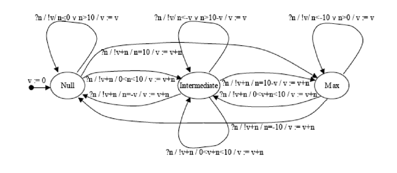
Figure 4: Example of an EFSM: counter with increment and decrement values.

Transitions are atomic and cannot be interrupted. Given an EFSM, if each variable and input parameter has a finite number of values (variables for booleans or for intervals of finite integers, for example), then there is a finite number of configurations, and hence there is a large equivalent (ordinary) FSM with configurations as states. Therefore, an EFSM with finite variable domains is a succinct representation of an FSM. Generally, constructing this FSM is not easy because of the reachability problem, i.e. the issue of determining if a configuration is reachable from the initial state. It is undecidable if the variable domains are infinite and PSPACE-complete otherwise.

A symbolic trace $t_{1},\ldots,t_{n}$ of an EFSM is a sequence of symbolic transitions such that $s_{t_{1}}=s_{0}$ and for $i=1,\ldots n-1$, $s^{\prime}_{t_{i}}=s_{t_{i+1}}$. A trace predicate is the condition on inputs which ensures the execution of a symbolic trace. Such a predicate is built by traversing the trace $t_{1},\ldots,t_{n}$ in the following way:

• the initial index of each variable $x$ is $0$, and for each variable $x$ there is an equation $x_{0}=v_{0}$,

• for $i=1\ldots n$, given transition $t_{i}$ with guard $G_{i}$, and action $A_{i}$:

  • guard $G_{i}$ is transformed into the formula $\tilde{G}_{i}$ where each variable of $G$ has been indexed by its current index, and the input parameter (if any) is indexed by $i$,

  • each assignment in $A_{i}$ of an expression $\,expr$ to some variable $x$ is transformed into an equation $x_{k+1}=\widetilde{expr}_{i}$ where $k$ is the current index of $x$ and $\widetilde{expr}_{i}$ is the expression $expr$ where each variable is indexed by its current index, and the input parameter (if any) is indexed by $i$,

  • the current indexes of all assigned variables are incremented,

• the trace predicate is the conjunction of all these formulae.

A symbolic trace is feasible if its predicate is satisfiable, i.e. there exist some sequence of input values that ensure that at each step of the trace, the guard of the symbolic transition is true. Such a sequence of inputs characterizes a trace of the EFSM. A configuration is reachable if there exists a trace leading to it.

EFSM testing methods must perform reachability analysis: to compute some input sequence that exercises a feature (trace, transition, state) of a given EFSM, a feasible symbolic trace leading to and covering this feature must be identified and its predicate must be solved. Depending on the kind of formula and expression allowed in guards and actions, different constraint solvers may be used [CGK⁺11, TGM11]. Some tools combine them with SAT-solvers, model checking techniques, symbolic evaluation methods including abstract interpretation, to eliminate some classes of clearly infeasible symbolic traces.

The notion of EFSM is very generic. The corresponding test generation problem is very similar to test generation for programs in general. The current methods address specific kinds of EFSM or SLTS. There are still a lot of open problems to improve the levels of generality and automation.

2.3.4 Classical methods in probabilistic and statistical testing

Drawing test cases at random is an old idea, which looks attractive at first sight. It turns out that it is difficult to estimate its detection power. Strong hypotheses on the IUT, on the types and distribution of faults, are necessary to draw conclusions from such test campaigns. Depending on authors and contexts, testing methods based on random selection of test cases are called: random testing, or probabilistic testing or statistical testing. These methods can be classified into three categories : those based on the input domain, those based on the environment, and those based on some knowledge of the behavior of the IUT.

In the first case, classical random testing (as studied in [DN81, DN84]) consists in selecting test data uniformly at random from the input domain of the program. In some variants, some knowledge on the input domain is exploited, for instance to focus on the boundary or limit conditions of the software being tested [Rei97, Nta01].

In the second case, the selection is based on an operational profile, i.e. an estimate of the relative frequency of inputs. Such testing methods are called statistical testing. They can serve as a statistical sampling method to collect failure data for reliability estimation (for a survey see [MFI⁺96]).

In the third case, some description of the behavior of the IUT is used. In [TFW91], the choice of the distribution on the input domain is guided either by some coverage criteria of the program and they call their method structural statistical testing, or by some specification and they call their method functional statistical testing.

Another approach is to perform random walks [Ald91] in the set of execution paths or traces of the IUT. Such testing methods were developed early in the area of communication protocols [Wes89, MP94]. In [Wes89], West reports experiments where random walk methods had good and stable error detection power. In [MP94], some class of models is identified, namely those where the underlying graph is symmetric, which can be efficiently tested by random walk exploration: under this strong condition, the random walk converges to the uniform distribution over the state space in polynomial time with respect to the size of the model. A general problem with all these methods is the impossibility, except for some very special cases, to assess the results of a test campaign, either in term of coverage or in term of fault detection.

3 Methods for approximation

In this section we classify the different approximations introduced in model checking and testing in two categories. Methods which approximate decision problems, based on some parameters, and methods which study approximate versions of the decision problems.

1. Approximate methods for decision, counting and learning problems. The goal is to define useful heuristics on practical inputs. SAT is the typical example where no polynomial algorithm exists assuming $P\neq NP$, but where useful heuristics are known. The search for abstraction methods by successive refinements follows the same approach.

2. Approximate versions of decision and learning problems relax the decision by introducing some error parameter $\varepsilon$. In this case, we may obtain efficient randomized algorithms, often based on statistics for these new approximate decision problems.

Each category is detailed in subsections below. First, we introduce the classes of efficient algorithms we will use to elaborate approximation methods.

3.1 Randomized algorithms and complexity classes

The efficient algorithms we study are mostly randomized algorithms which operate in polynomial time. They use an extra instruction, flip a coin, and we obtain $0$ or $1$ with probability $\frac{1}{2}$. As we make $n$ random flips, the probabilistic space $\Omega$ consists of all binary sequences of length $n$, each with probability $\frac{1}{2^{n}}$. We want to decide if $x\in L\subseteq\Sigma^{*}$, such that the probability of getting the wrong answer is less than $\frac{c}{2^{n}}$ for some fixed constant $c$, i.e. exponentially small.

Definition 3

An algorithm $\mathcal{A}$ is Bounded-error Probabilistic Polynomial-time (BPP), for a language $L\subseteq\Sigma^{*}$ if $\mathcal{A}$ is in polynomial time and:

• if $x\in L$ then $\mathcal{A}$ accepts $x$ with probability greater then $2/3$,

• if $x\not\in L$ then $\mathcal{A}$ rejects $x$ with probability greater then $2/3$.

The class BPP consists of all languages $L$ which admit a bounded-error probabilistic polynomial time algorithm.

In this definition, we can replace $2/3$ by any value strictly greater than $1/2$, and obtain an equivalent definition. In some cases, $2/3$ is replaced by $1/2+\varepsilon$ or by $1-\delta$ or by $1-1/n^{k}$. If we modify the second condition of the previous defintion by: if $x\not\in L$ then $\mathcal{A}$ rejects $x$ with probability 1, we obtain the class RP, Randomized Polynomial time.

We recall the notion of a p-predicate, used to define the class $\mathsf{NP}$ of decision problems which are verifiable in polynomial time.

Definition 4

A p-predicate $R$ is a binary relation between words such that there exist two polynomials $p,q$ such that:

• for all ${\bf x},{\bf y}\in\Sigma^{*}$, $R({\bf x},{\bf y})$ implies that $\mid{\bf y}\mid\leq p(\mid{\bf x}\mid)$;

• for all ${\bf x},{\bf y}\in\Sigma^{*}$ , $R({\bf x},{\bf y})$ is decidable in time $q(\mid{\bf x}\mid)$.

A decision problem $A$ is in the class $\mathsf{NP}$ if there is a p-predicate $R$ such that for all $x$, $x\in A$ iff $\exists yR(x,y)$. Typical examples are $\mathsf{SAT}$ for clauses or $\mathsf{CLIQUE}$ for graphs. For $\mathsf{SAT}$, the input $x$ is a set of clauses, $y$ is a valuation and $R(x,y)$ if $y$ satisfies $x$. For $\mathsf{CLIQUE}_{k}$, the input $x$ is a graph, $y$ is a subset of size $k$ of the nodes and $R(x,y)$ if $y$ is a clique of $x$, i.e. if all pairs of nodes in $y$ are connected by an edge.

One needs a precise notion of approximation for a counting function $F:\Sigma^{*}\rightarrow N$ using an efficient randomized algorithm whose relative error is bounded by $\varepsilon$ with high probability, for all $\varepsilon$. It is used in section 4.5.3 to approximate probabilities.

Definition 5

An algorithm $\mathcal{A}$ is a Polynomial-time Randomized Approximation Scheme (PRAS) for a function $F:\Sigma^{*}\rightarrow\mathbb{N}$ if for every $\varepsilon$ and x,

$$\Pr\{\mathcal{A}({\bf x},\varepsilon)\in[(1-\varepsilon).F({\bf x}),(1+\varepsilon).F({\bf x})]\}~{}\geq~{}\frac{2}{3}$$

and $\mathcal{A}({\bf x},\varepsilon)$ stops in polynomial time in $\mid{\bf x}\mid$. The algorithm $\mathcal{A}$ is a Fully Polynomial time Randomized Approximation Schema (FPRAS), if the time of computation is also polynomial in $1/\varepsilon$. The class PRAS (resp. FPRAS) consists of all functions $F$ which admits a PRAS (resp. FPRAS) .

If the algorithm $\mathcal{A}$ is deterministic, one speaks of an $PAS$ and of a $FPAS$. A $PRAS(\delta)$ (resp. $FPRAS(\delta)$), is an algorithm $\mathcal{A}$ which outputs a value $\mathcal{A}({\bf x},\varepsilon,\delta)$ such that:

$$\Pr\{\mathcal{A}({\bf x},\varepsilon,\delta)\in[(1-\varepsilon).F({\bf x}),(1+\varepsilon).F({\bf x})]\}~{}\geq~{}1-\delta$$

and whose time complexity is also polynomial in $\log(1/\delta)$. The error probability is less than $\delta$ in this model. In general, the probability of success can be amplified from $2/3$ to $1-\delta$ at the cost of extra computation of length polynomial in $\log(1/\delta)$.

Definition 6

A counting function $F$ is in the class $\#$P if there exists a p-predicate $R$ such that for all $x$, $F(x)=\mid\{y:(x,y)\in R\}\mid$.

If $A$ is an $\mathsf{NP}$ problem, i.e. the decision problem on input $x$ which decides if there exists $y$ such that $R(x,y)$ for a p-predicate $R$, then $\#A$ is the associated counting function, i.e. $\#A(x)=\mid\{y:(x,y)\in R\}\mid$. The counting problem $\#SAT$ is $\#$P-complete and not approximable (modulo some complexity conjecture). On the other hand $\#DNF$ is also $\#$P-complete but admits an $FPRAS$ [KL83].

3.2 Approximate methods for satisfiability, equivalence, counting and learning

Satisfiability decides given a model $\mathcal{M}$ and a formula $\psi$, whether $\mathcal{M}$ satisfies a formula $\psi$. Equivalence decides given two models $\mathcal{M}$ and $\mathcal{M}^{\prime}$, whether they satisfy the same class of formulas. Counting associates to a formula $\psi$, the number of models $\mathcal{M}$ which satisfy a formula $\psi$. Learning takes a black box which defines an unknown function $f$ and tries to find from samples $x_{i},y_{i}=f(x_{i})$.

3.2.1 Approximate satisfiability and abstraction

To verify that a model $\mathcal{M}$ satisfies a formula $\psi$ , abstraction can be used for constructing approximations of $\mathcal{M}$ that are sufficient for checking $\psi$. This approach goes back to the notion of Abstract Interpretation, a theory of semantic approximation of programs introduced by Cousot et al.[CC77], which constructs elementary embeddings that suffice to decide properties of programs. A classical example is multiplication, where modular arithmetic is the basis of the abstraction. It has been applied in static analysis to find sound, finite, and approximate representations of a program.

In the framework of model checking, reduction by abstraction consists in approximating infinite or very large finite transition systems by finite ones, on which existing algorithms designed for finite verification are directly applicable. This idea was first introduced by Clarke et al. [EMCL94]. Graf and Saidi [GS97] have then proposed the predicate abstraction method where abstractions are automatically obtained, using decision procedures, from a set of predicates given by the user. When the resulting abstraction is not adequate for checking $\psi$, the set of predicates must be revised. This approach by abstraction refinement has been recently systematized, leading to a quasi automatic abstraction discovery method known as Counterexample-Guided Abstraction Refinement (CEGAR) [CGJ⁺03]. It relies on the iteration of three kinds of steps: abstraction construction, model checking of the abstract model, abstraction refinement, which, when it terminates, states whether the original model satifies the formula.

This section starts with the notion of abstraction used in model checking, based on the pioneering paper by Clarke et al.. Then, we present the principles of predicate abstraction and abstraction refinement.

In [EMCL94], Clarke and al. consider transition systems $\mathcal{M}$ where atomic propositions are formulas of the form $v=d$, where $v$ is a variable and $d$ is a constant. Given a set of typed variable declarations $v_{1}:T_{1},\ldots,v_{n}:T_{n}$, states can be identified with n-tuples of values for variables, and the labeling function $L$ is just defined by $L(s)=\{s\}$. On such systems, abstractions can be defined by a surjection for each variable into a smaller domain. It reduces the size of the set of states. Transitions are then stated between the resulting equivalence classes of states as defined below.

Definition 7

([EMCL94]) Let $\mathcal{M}$ be a transition system, with set of states $S$, transition relation $R$, and a set of initial states $I\subseteq S$. An abstraction for $\mathcal{M}$ is a surjection $h:S\rightarrow\widehat{S}$. A transition system $\widehat{\mathcal{M}}=(\widehat{S},\widehat{I},\widehat{R},\widehat{L})$ approximates $\mathcal{M}$ with respect to $h$ ($\mathcal{M}\sqsubseteq_{h}\widehat{\mathcal{M}}$ for short) if $h(I)\subseteq\widehat{I}$ and $(h(s),h(s^{\prime}))\in\widehat{R}$ for all $(s,s^{\prime})\in R$.

Such an approximation is called an over approximation and is explicitly given in [EMCL94] from a given logical representation of $\mathcal{M}$.

Now, let $\widehat{\mathcal{M}}$ be an approximation of $\mathcal{M}$. Suppose that $\widehat{\mathcal{M}}\models\Theta$. What can we conclude on the concrete model $\mathcal{M}$? First consider the following transformations $\mathcal{C}$ and $\mathcal{D}$ between $\mathrm{CTL}^{*}$ formulas on $\mathcal{M}$ and their approximation on $\widehat{\mathcal{M}}$. These transformations preserve boolean connectives, path quantifiers, and temporal operators, and act on atomic propositions as follows:

$$\mathcal{C}(\widehat{v}=\widehat{d})\stackrel{{\scriptstyle\mbox{\tiny def}}}{{=}}\bigvee_{d:h(d)=\widehat{d}}(v=d),\qquad\mathcal{D}(v=d)\stackrel{{\scriptstyle\mbox{\tiny def}}}{{=}}(\widehat{v}=h(d)).$$

Denote by $\boldsymbol{\forall}\mathrm{CTL}^{*}$ and $\boldsymbol{\exists}\mathrm{CTL}^{*}$ the universal fragment and the existential fragment of $\mathrm{CTL}^{*}$. The following theorem gives correspondences between models and their approximations.

Theorem 2 ([EMCL94])

Let $\mathcal{M}=(S,I,R,L)$ be a transition system. Let $h:S\rightarrow\widehat{S}$ be an abstraction for $\mathcal{M}$, and let $\widehat{\mathcal{M}}$ be such that $\mathcal{M}\sqsubseteq_{h}\widehat{\mathcal{M}}$. Let $\Theta$ be a $\boldsymbol{\forall}\mathrm{CTL}^{*}$ formula on $\widehat{M}$, and $\Theta^{\prime}$ be a $\boldsymbol{\exists}\mathrm{CTL}^{*}$ formula on $M$. Then

$$\widehat{\mathcal{M}}\models\Theta\implies\mathcal{M}\models\mathcal{C}(\Theta)\quad\text{and}\quad\mathcal{M}\models\Theta^{\prime}\implies\widehat{\mathcal{M}}\models\mathcal{D}(\Theta^{\prime}).$$

Abstraction can also be used when the target structure does not follow the original source signature. In this case, some specific new predicates define the target structure and the technique has been called predicate abstraction by Graf et al. [GS97]. The analysis of the small abstract structure may suffice to prove a property of the concrete model and the authors define a method to construct abstract state graphs from models of concurrent processes with variables on finite domains. In these models, transitions are labelled by guards and assignments. The method starts from a given set of predicates on the variables. The choice of these predicates is manual, inspired by the guards and assignments occurring on the transitions. The chosen predicates induce equivalence classes on the states. The computation of the successors of an abstract state requires theorem proving. Due to the number of proofs to be performed, only relatively small abstract graphs can be constructed. As a consequence, the corresponding approximations are often rather coarse. They must be tuned, taking into account the properties to be checked.

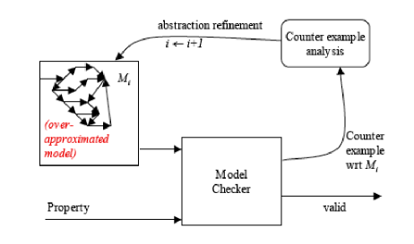
Figure 5: CEGAR:Counterexample-Guided Abstraction Refinement.

We now explain how to use abstraction refinement in order to achieve $\forall CTL^{*}$ model checking: for a concrete structure $\mathcal{M}$ and an $\forall CTL^{*}$ formula $\psi$, we would like to check if $M\models\psi$. The methodology of the counterexample-guided abstraction refinement [CGJ⁺03] consists in the following steps:

• Generate an initial abstraction $\widehat{\mathcal{M}}$.

• Model check the abstract structure. If the check is affirmative, one can conclude that $\mathcal{M}\models\psi$; otherwise, there is a counterexample to $\widehat{\mathcal{M}}\models\psi$. To verify if it is a real counterexample, one can check it on the original structure; if the answer is positive, it is reported it to the user; if not, one proceeds to the refinement step.

• Refine the abstraction by partitioning equivalence classes of states so that after the refinement, the new abstract structure does not admit the previous counterexample. After refining the abstract structure, one returns to the model checking step.

The above approaches are said to use over approximation because the reduction induced on the models introduces new paths, while preserving the original ones. A notion of under approximation is used in bounded model checking where paths are restricted to some finite lengths. It is presented in section 4.1. Another approach using under approximation is taken in [MS07] for the class of models with input variables. The original model is coupled with a well chosen logical circuit with $m<n$ input variables and $n$ outputs. The model checking of the new model may be easier than the original model checking, as fewer input variables are considered.

3.2.2 Uniform generation and counting

In this section we describe the link between generating elements of a set $S$ and counting the size of $S$, first in the exact case and then in the approximate case. The exact case is used in section 4.4.2 and the approximate case is later used in section 4.5.3 to approximate probabilities.

Exact case. Let $S_{n}$ be a set of combinatorial objects of size $n$. There is a close connection between having an explicit formula for $\mid S_{n}\mid$ and a uniform generator for objects in $S_{n}$. Two major approaches have been developed for counting and drawing uniformly at random combinatorial structures: the Markov Chain Monte-Carlo approach (see e.g. the survey [JS96]) and the so-called recursive method, as described in [FZC94] and implemented in [Thi04]. Although the former is more general in its applications, the latter is particularly efficient for dealing with the so-called decomposable combinatorial classes of Structures, namely classes where structures are formed from a set $\mathcal{Z}$ of given atoms combined by the following constructions:

$$+,\times,\textsc{Seq},\textsc{PSet},\textsc{MSet},\textsc{Cyc}$$

respectively corresponding to disjoint union, Cartesian product, finite sequence, multiset, set, directed cycles. It is possible to state cardinality constraints via subscripts (for instance $\textsc{Seq}_{\leq 3}$). These structures are called decomposable structures. The size of an object is the number of atoms it contains.

Example 1

Trees :

• The class $\mathcal{B}$ of binary trees can be specified by the equation $\mathcal{B}=\mathcal{Z}+(\mathcal{B}\times\mathcal{B})$ where $\mathcal{Z}$ denotes a fixed set of atoms.

• An example of a structure in $\mathcal{B}$ is $(\mathcal{Z}\times(\mathcal{Z}\times\mathcal{Z}))$. Its size is 3.

• For non empty ternary trees one could write $\mathcal{T}=\mathcal{Z}+\textsc{Seq}_{=3}(\mathcal{T})$

The enumeration of decomposable structures is based on generating functions. Let $C_{n}$ the number of objects of $C$ of size $n$, and the following generating function:

$$C(z)=\sum_{n\leq 0}C_{n}z^{n}$$

Decomposable structures can be translated into generating functions using classical results of combinatorial analysis. A comprehensive dictionary is given in [FZC94]. The main result on counting and random generation of decomposable structures is:

Theorem 3

Let $C$ be a decomposable combinatorial class of structures. Then the counts $\{C_{j}|j=0\ldots n\}$ can be computed in $O(n^{1+\varepsilon})$ arithmetic operations, where $\varepsilon$ is a constant less than $1$. In addition, it is possible to draw an element of size $n$ uniformly at random in $O(n\log n)$ arithmetic operations in the worst case.

A first version of this theorem, with a computation of the counting sequence $\{C_{j}|j=0\ldots n\}$ in $O(n^{2})$ was given in [FZC94]. The improvement to $O(n^{1+\varepsilon})$ is due to van der Hoeven [vdH02].

This theory has led to powerful practical tools for random generation [Thi04]. There is a preprocessing step for the construction of the $\{C_{j}|j=0\ldots n\}$ tables . Then the drawing is performed following the decomposition pattern of $C$, taking into account the cardinalities of the involved sub-structures. For instance, in the case of binary trees, one can uniformly generate binary trees of size $n+1$ by generating a random $k\leq n$, with probability

$$p(k)=\frac{|\mathcal{B}_{k}|.|\mathcal{B}_{n-k}|}{|\mathcal{B}_{n}|}$$

where $\mathcal{B}_{k}$ is the set of binary trees of size $k$. A tree of size $n+1$ is decomposed into a subtree on the left side of the root of size $k$ and into a subtree on the right side of the root of size $n-k$. One recursively applies this procedure and generates a binary tree with $n$ atoms following a uniform distribution on $\mathcal{B}_{n}$.

Approximate case. In the case of a hard counting problem, i.e. when $\mid S_{n}\mid$ does not have an explicit formula, one can introduce a useful approximate version of counting and uniform generation. Suppose the objects are witnesses of a p-predicate, i.e. they can be recognized in polynomial time.

Approximate counting $S$ can be reduced to approximate uniform generation of $y\in S$ and conversely approximate uniform generation can be reduced to approximate counting, for self-reducible sets. Self-reducible sets guarantees that a solution for an instance of size $n$ depends directly from solutions for instances of size $n-1$. For example, in the case of SAT, a valuation on $n$ variables $p_{1},...,p_{n}$ on an instance $x$ is either a valuation of an instance $x_{1}$ of size $n-1$ where $p_{n}=1$ or a valuation of an instance $x_{0}$ of size $n-1$ where $p_{n}=0$. Thus the p-predicate for SAT is a self-reducible relation.

To reduce approximate counting to approximate uniform generation, let $S_{\sigma}$ be the set $S$ where the first letter of $y$ is $\sigma$, and $p_{\sigma}=\frac{\mid S_{\sigma}\mid}{\mid S\mid}$. For self-reducible sets $\mid S_{\sigma}\mid$ can be recursively approximated using the same technique. Let $p_{\sigma.\sigma^{\prime}}=\frac{\mid S_{\sigma.\sigma^{\prime}}\mid}{\mid S_{\sigma}\mid}$ and so on, until one reaches $\mid S_{\sigma_{1},...,\sigma_{m}}\mid$ if $m=|y|-1$, which can be directly computed. Then

$$\mid S\mid=\frac{\mid S_{\sigma_{1},...,\sigma_{m}}\mid}{p_{\sigma_{1}}.p_{\sigma_{1}.\sigma_{2}},...,p_{\sigma_{1},...,\sigma_{m-1}}}$$

Let $\widehat{p_{\sigma}}$ be the estimated measure for $p_{\sigma}$ obtained with the uniform generator for $y$. The $p_{\sigma_{1},...,\sigma_{i}}$ can be replaced by their estimates and leading to an estimator for $\mid S\mid$.

Conversely, one can reduce approximate uniform generation to approximate counting. Compute $\mid S_{\sigma}\mid$ and $\mid S\mid$. Suppose $\Sigma=\{0,1\}$ and let $p_{0}=\frac{\mid S_{0}\mid}{\mid S\mid}$. Generate $0$ with probability $p_{0}$ and $1$ with probability $1-p_{0}$ and recursively apply the same method. If one obtains $0$ as the first bit, one sets $p_{00}=\frac{\mid S_{00}\mid}{\mid S_{0}\mid}$ and generates $0$ as the next bit with probability $p_{00}$ and $1$ with probability $1-p_{00}$, and so on. One obtains a string $y\in S$ with an approximate uniform distribution.

3.2.3 Learning

In the general setting, given a black box, i.e. an unknown function $f$, and samples $x_{i},y_{i}=f(x_{i})$ for $i=1,...,N$, one wishes to find $f$. Classical learning theory distinguishes between supervised and unsupervised learning. In supervised learning $f$ is one function among a class ${\cal F}$ of given functions. In unsupervised learning, one tries to find $g$ as the best possible function.

Learning models suppose membership queries, i.e. positive and negative examples, i.e. given $x$, an oracle produces $f(x)$ in one step. Some models assume more general queries such as conjecture queries: given an hypothesis $g$, an oracle answers YES if $f=g$, else produces an $x$ where $f$ and $g$ differ. For example, let $f$ be a function $\Sigma^{*}\rightarrow\{0,1\}$ where $\Sigma$ is a finite alphabet. It describes a language $L=\{x\in\Sigma^{*},~{}~{}f(x)=1\}\subseteq\Sigma^{*}$. On the basis of membership and conjecture Queries, one tries to output $g=f$.

Angluin’s Learning algorithm for regular sets

The learning model is such that the teacher answers membership queries and conjecture queries. Angluin’s algorithm shows how to learn any regular set, i.e. any function $\Sigma^{*}\rightarrow\{0,1\}$, which is the characteristic function of a regular set. It finds $f$ exactly, and the complexity of the procedure depends polynomially $O(m.n^{2})$ on two parameters: $n$ the size of the minimum automaton for $f$ and $m$ the maximum length of counter examples returned by the conjecture queries. Moreover there are at most $n$ conjecture Queries.

Learning without reset

The Angluin model supposes a reset operator, similar to the reliable reset of section 2.3.1, but [RS93] showed how to generalize the Angluin model without reset. As seen in Section 2.3.1, a homing sequence is a sequence which uniquely identifies the state after reading the sequence. Every minimal deterministic finite automaton has a homing sequence $\sigma$.

The procedure runs $n$ copies of Angluin’s algorithm, $L_{1},...,L_{n}$, where $L_{i}$ assumes that $s_{i}$ is the initial state. After a membership query in $L_{i}$, one applies the homing sequence $\sigma$, which leads to state $s_{k}$. One leaves $L_{i}$ and continues in $L_{k}$.

3.3 Methods for approximate decision problems

In the previous section, we considered approximate methods for decision, counting and learning problems. We now relax the decision and learning problems in order to obtain more efficient approximate methods.

3.3.1 Property testing

Property testing is a statistics based approximation technique to decide if either an input satisfies a given property, or is far from any input satisfying the property, using only few samples of the input and a specific distance between inputs. It is later used in section 4.2. The idea of moving the approximation to the input was implicit in Program Checking [BK95, BLR93, RS96], in Probabilistically Checkable Proofs (PCP) [AS98], and explicitly studied for graph properties under the context of property testing [GGR98]. The class of sublinear algorithms has similar goals: given a massive input, a sublinear algorithm can approximately decide a property by sampling a tiny fraction of the input. The design of sublinear algorithms is motivated by the recent considerable growth of the size of the data that algorithms are called upon to process in everyday real-time applications, for example in bioinformatics for genome decoding or in Web databases for the search of documents. Linear-time, even polynomial-time, algorithms were considered to be efficient for a long time, but this is no longer the case, as inputs are vastly too large to be read in their entirety.

Given a distance between objects, an $\varepsilon$-tester for a property $P$ accepts all inputs which satisfy the property and rejects with high probability all inputs which are $\varepsilon$-far from inputs that satisfy the property. Inputs which are $\varepsilon$-close to the property determine a gray area where no guarantees exists. These restrictions allow for sublinear algorithms and even $O(1)$ time algorithms, whose complexity only depends on $\varepsilon$.

Let $\mathbf{K}$ be a class of finite structures with a normalized distance $\mathsf{dist}$ between structures, i.e. $\mathsf{dist}$ lies in $[0,1]$. For any $\varepsilon>0$, we say that $U,U^{\prime}\in\mathbf{K}$ are $\varepsilon$-close if their distance is at most $\varepsilon$. They are $\varepsilon$-far if they are not $\varepsilon$-close. In the classical setting, satisfiability is the decision problem whether $U\models P$ for a structure $U\in\mathbf{K}$ and a property $P\subset\mathbf{K}$. A structure $U\in\mathbf{K}$ $\varepsilon$-satisfies $P$, or $U$ is $\varepsilon$-close to $\mathbf{K}$ or $U\models_{\varepsilon}P$ for short, if $U$ is $\varepsilon$-close to some $U^{\prime}\in\mathbf{K}$ such that $U^{\prime}\models P$. We say that $U$ is $\varepsilon$-far from $\mathbf{K}$ or $U\not\models_{\varepsilon}P$ for short, if $U$ is not $\varepsilon$-close to $\mathbf{K}$.

Definition 8 (Property tester [GGR98])

Let $\varepsilon>0$. An $\varepsilon$-tester for a property $P\subseteq\mathbf{K}$ is a randomized algorithm $A$ such that, for any structure $U\in\mathbf{K}$ as input:
(1) If $U\models P$, then $A$ accepts;
(2) If $U\not\models_{\varepsilon}P$, then $A$ rejects with probability at least $2/3$.

A query to an input structure $U$ depends on the model for accessing the structure. For a word $w$, a query asks for the value of $w[i]$, for some $i$. For a tree $T$, a query asks for the value of the label of a node $i$, and potentially for the label of its parent and its $j$-th successor, for some $j$. For a graph a query asks if there exists an edge between nodes $i$ and $j$. We also assume that the algorithm may query the input size. The query complexity is the number of queries made to the structure. The time complexity is the usual definition, where we assume that the following operations are performed in constant time: arithmetic operations, a uniform random choice of an integer from any finite range not larger than the input size, and a query to the input.

Definition 9

A property $P\subseteq\mathbf{K}$ is testable, if there exists a randomized algorithm $A$ such that, for every real $\varepsilon>0$ as input, $A(\varepsilon)$ is an $\varepsilon$-tester of $P$ whose query and time complexities depend only on $\varepsilon$ (and not on the input size).

Tools based on property testing use an approximation on inputs which allows to:

1. Reduce the decision of some global properties to the decision of local properties by sampling,

2. Compress a structure to a constant size sketch on which a class of properties can be approximated.

We detail some of the methods on graphs, words and trees.

Graphs

In the context of undirected graphs [GGR98], the distance is the (normalized) Edit distance on edges: the distance between two graphs on $n$ nodes is the minimal number of edge-insertions and edge-deletions needed to modify one graph into the other one. Let us consider the adjacency matrix model. Therefore, a graph $G=(V,E)$ is said to be $\varepsilon$-close to another graph $G^{\prime}$, if $G$ is at distance at most $\varepsilon n^{2}$ from $G^{\prime}$, that is if $G$ differs from $G^{\prime}$ in at most $\varepsilon n^{2}$ edges.

In several cases, the proof of testability of a graph property on the initial graph is based on a reduction to a graph property on constant size but random subgraphs. This was generalized for every testable graph properties by  [GT03]. The notion of $\varepsilon$-reducibility highlights this idea. For every graph $G=(V,E)$ and integer $k\geq 1$, let $\Pi$ denote the set of all subsets $\pi\subseteq V$ of size $k$. Denote by $G_{\pi}$ the vertex-induced subgraph of $G$ on $\pi$.

Definition 10

Let $\varepsilon>0$ be a real, $k\geq 1$ an integer, and $\phi,\psi$ two graph properties. Then $\phi$ is $(\varepsilon,k)$-reducible to $\psi$ if and only if for every graph $G$,

$$G\models\phi \implies \forall\pi\in\Pi,\ G_{\pi}\models\psi,$$

$$G\not\models_{\varepsilon}\phi \implies \Pr_{\pi\in\Pi}[G_{\pi}\not\models\psi]\geq 2/3.$$

Note that the second implication means that if $G$ is $\varepsilon$-far to all graphs satisfying the property $\phi$, then with probability at least $2/3$ a random subgraph on $k$ vertices does not satisfy $\psi$.

Therefore, in order to distinguish between a graph satisfying $\phi$ to another one that is far from all graphs satisfying $\phi$, we only have to estimate the probability $\Pr_{\pi\in\Pi}[G_{\pi}\models\psi]$. In the first case, the probability is $1$, and in the second it is at most $1/3$. This proves that the following generic test is an $\varepsilon$-tester:

Generic Test$(\psi,\varepsilon,k)$
1. Input: A graph $G=(V,E)$ 2. Generate uniformly a random subset $\pi\subseteq V$ of size $k$ 3. Accept if $G_{\pi}\models\psi$ and reject otherwise

Proposition 1

If for every $\varepsilon>0$, there exists $k_{\varepsilon}$ such that $\phi$ is $(\varepsilon,k_{\varepsilon})$-reducible to $\psi$, then the property $\phi$ is testable. Moreover, for every $\varepsilon>0$, Generic Test$(\psi,\varepsilon,k_{\varepsilon})$ is an $\varepsilon$-tester for $\phi$ whose query and time complexities are in $(k_{\varepsilon})^{2}$.

In fact, there is a converse of that result, and for instance we can recast the testability of $c$-colorability [GGR98, AK02] in terms of $\varepsilon$-reducibility. Note that this result is quite surprising since $c$-colorability is an NP-complete problem for $c\geq 3$.

Theorem 4 ([AK02])

For all $c\geq 2$, $\varepsilon>0$, $c$-colorability is $(\varepsilon,O((c\ln c)/\varepsilon^{2}))$-reducible to $c$-colorability.

Words and trees

Property testing of regular languages was first considered in [AKNS00] for the Hamming distance, and then extended to languages recognizable by bounded width read-once branching programs [New02], where the Hamming distance between two words is the minimal number of character substitutions required to transform one word into the other. The (normalized) edit distance between two words (resp. trees) of size $n$ is the minimal number of insertions, deletions and substitutions of a letter (resp. node) required to transform one word (resp. tree) into the other, divided by $n$. When words are infinite, the distance is defined as the superior limit of the distance of the respective prefixes.

[MdR07] considered the testability of regular languages on words and trees under the edit distance with moves, that considers one additional operation: moving one arbitrary substring (resp. subtree) to another position in one step. This distance seems to be more adapted in the context of property testing, since their tester is more efficient and simpler than the one of [AKNS00], and can be generalized to tree regular languages.

[FMdR10] developed a statistical embedding of words which has similarities with the Parikh mapping [Par66]. This embedding associate to every word a sketch of constant size (for fixed $\varepsilon$) which allows to decide any property given by some regular grammar or even some context-free grammar. This embedding has other implications that we will develop further in Section 4.2.3.

3.3.2 PAC and statistical learning

The Probably Approximately Correct (PAC) learning model, introduced by Valiant [Val84] is a framework to approximately learn an unknown function $f$ in a class $\cal{F}$, such that each $f$ has a finite representation, i.e. a formula which defines $f$. The model supposes positive and negative samples along a distribution $\cal{D}$, i.e. values $x_{i},f(x_{i})$ for $i=1,2,...,N$. The learning algorithm proposes a function $h$ and the error between $f$ and $h$ along the distribution $\cal{D}$ is:

$$error(h)=\Pr_{x\in\cal{D}}[f(x)\neq h(x)]$$

A class $\cal{F}$ of functions $f$ is PAC-learnable if there is a randomized algorithm such that for all $f\in\cal{F},\varepsilon,\delta,\cal{D}$, it produces with probability greater than $1-\delta$, an estimate $h$ for $f$ such that $error(h)\leq\varepsilon$. It is efficiently PAC-learnable if the algorithm is polynomial in $N,\frac{1}{\varepsilon},\frac{1}{\delta},size(f)$, where $size(f)$ is the size of the finite representation of $f$. Such learning methods are independent of the distribution $\cal{D}$, and are used in black box checking in section 4.3 to verify a property of a black box by learning a model.

The class $\cal{H}$ of the functions $h$ is called the Hypothesis space and the class is properly learnable if $\cal{H}$ is identical to $\cal{F}$:

• Regular languages are PAC-learnable. Just replace in Angluin’s model, the conjecture queries by PAC queries, i.e. samples from a distribution $\cal{D}$. Given a proposal $L^{\prime}$ for $L$, we take N samples along $\cal{D}$ and may obtain a counterexample, i.e. an element $x$ on which $L$ and $L^{\prime}$ disagree. If $n$ is the minimum number of states of the unknown $L$, then Angluin’s algorithm with at most

  $$N=O((n+1/\varepsilon).(n\ln(1/\delta)+n^{2})$$

  samples can replace the $n$ conjecture queries and guarantee with probability at least $1-\delta$ that the error is less than $\varepsilon$.

• $k$-DNF and $k$-CNF are learnable but it is not known whether CNF or DNF are learnable.

The Vapnik-Chernovenkis (VC) dimension [VC81] of a class $\cal{F}$, denoted $VC(\cal{F})$ is the largest cardinality $d$ of a sample set $S$ that is shattered by $\cal{F}$, i.e. such that for every subset $S^{\prime}\subseteq S$ there is an $f\in\cal{F}$ such that $f(x)=a$ for $x\in S^{\prime}$, $f(x)=b$ for $x\in S-S^{\prime}$ and $a\neq b$.

A classical result of [BEHW89, KV94] is that if $d$ is finite then the class is PAC learnable. If $N\geq O(\frac{1}{\varepsilon}.\log\frac{1}{\delta}+\frac{d}{\varepsilon}.\log\frac{1}{{}_{e}ps})$, then any $h$ which is consistent with the samples, i.e. gives the same result as $f$ on the random samples, is a good estimate. Statistical learning [Vap83] generalizes this approach from functions to distributions.

4 Applications to model checking and testing

4.1 Bounded and unbounded model checking

Recall that the Model Checking problem is to decide, given a transition system $\mathcal{M}$ with an initial state $s_{0}$ and a temporal formula $\varphi$ whether $\mathcal{M},s_{0}\models\varphi$, i.e. if the system $\mathcal{M}$ satisfies the property defined by $\varphi$. Bounded model checking introduced in [BCCZ99b] is a useful method for detecting errors, but incomplete in general for efficiency reasons: it may be intractable to ensure that a property is satisfied. For example, if we consider some safety property expressed by a formula $\varphi=\mathbf{G}p$, $\mathcal{M},s_{0}\models\mathbf{\forall}\varphi$ means that all initialized paths in $\mathcal{M}$ satisfy $\varphi$, and $\mathcal{M},s_{0}\models\mathbf{\exists}\varphi$ means that there exists an initialized path in $\mathcal{M}$ which satisfies $\varphi$. Therefore, finding a counterexample to the property $\mathbf{G}p$ corresponds to the question whether there exists a path that is a witness for the property $\mathbf{F}\neg p$.

The basic idea of bounded model checking is to consider only a finite prefix of a path that may be a witness to an existential model checking problem. The length of the prefix is restricted by some bound $k$. In practice, one progressively increases the bound, looking for witnesses in longer and longer execution paths. A crucial observation is that, though the prefix of a path is finite, it represents an infinite path if there is a back loop to any of the previous states. If there is no such back loop, then the prefix does not say anything about the infinite behavior of the path beyond state $s_{k}$.

The $k$-bounded semantics of model checking is defined by considering only finite prefixes of a path, with length $k$, and is an approximation to the unbounded semantics. We will denote satisfaction with respect to the $k$-bounded semantics by $\models_{k}$. The main result of bounded model checking is the following.

Theorem 5

Let $\varphi$ be an LTL formula and $\mathcal{M}$ be a transition system. Then $\mathcal{M}\models\mathbf{\exists}\varphi$ iff there exists $k=0(|\mathcal{M}|.2^{|\varphi|})$ such that $\mathcal{M}\models_{k}\mathbf{\exists}\varphi$.

Given a model checking problem $\mathcal{M}\models\mathbf{\exists}\varphi$, a typical application of BMC starts at bound $0$ and increments the bound $k$ until a witness is found. This represents a partial decision procedure for model checking problems:

• if $\mathcal{M}\models\mathbf{\exists}\varphi$, a witness of length $k$ exists, and the procedure terminates at length $k$.

• if $\mathcal{M}\not\models\mathbf{\exists}\varphi$, the procedure does not terminate.

For every finite transition system $\mathcal{M}$ and LTL formula $\phi$, there exists a number $k$ such that the absence of errors up to $k$ proves that $\mathcal{M}\models\mathbf{\forall}\phi$. We call $k$ the completeness treshold of $\mathcal{M}$ with respect to $\phi$. For example, the completeness treshold for a safety property expressed by a formula $\mathbf{G}p$ is the minimal number of steps required to reach all states: it is the longest “shortest path” from an initial state to any reachable state.

In the case of unbounded model checking, one can formulate the check for property satisfaction as a SAT problem. A general SAT approach [ABE00b] can be used for reachability analysis, when the binary relation $R$ is represented by a Reduced Boolean Circuit (RBC), a specific logical circuit with $\wedge,\neg,\leftrightarrow$. One can associate a SAT formula with the binary relation $R$ and each $R^{i}$ which defines the states reachable at stage $i$ from $s_{0}$, i.e. $R^{0}=\{s_{0}\}$, $R^{i+1}=\{s:\exists vR^{i}(v)\wedge vRs\}$. Reachability analysis consists in computing unary sets $T^{i}$, for $i=1,...,m$:

• $T^{i}$ is the set of states reachable at stage $i$ which satisfy a predicate $Bad$, i.e. $\exists s(Bad(s)\wedge R^{i}(s))$,

• compute $T^{i+1}$ and check if $T^{i}\leftrightarrow T^{i+1}$.

In some cases, one may have a more succinct representation of the transitive closure of $R$. A $SAT$ solver is used to perform all the decisions.

4.1.1 Translation of BMC to SAT

It remains to show how to reduce bounded model checking to propositional satisfiability. This reduction enables to use efficient propositional SAT solvers to perform model checking. Given a transition system $\mathcal{M}=(S,I,R,L)$ where $I$ is the set of initial states, an LTL formula $\varphi$ and a bound $k$, one can construct a propositional formula $[\mathcal{M},\varphi]_{k}$ such that:

$$\mathcal{M}\models_{k}\mathbf{\exists}\varphi\mbox{ iff }[\mathcal{M},\varphi]_{k}\mbox{ is satisfiable}$$

Let $(s_{0},\dots,s_{k})$ the finite prefix, of length $k$, of a path $\sigma$. Each $s_{i}$ represents a state at time step $i$ and consists of an assignment of truth values to the set of state variables. The formula $[\mathcal{M},\varphi]_{k}$ encodes constraints on $(s_{0},\dots,s_{k})$ such that $[\mathcal{M},\varphi]_{k}$ is satisfiable iff $\sigma$ is a witness for $\varphi$.

The first part $[\mathcal{M}]_{k}$ of the translation is a propositional formula that forces $(s_{0},\dots,s_{k})$ to be a path starting from an initial state: $[\mathcal{M}]_{k}=I(s_{0})\wedge\bigwedge_{i=0}^{k-1}R(s_{i},s_{i+1})$.

The second part $[\varphi]_{k}$ is a propositional formula which means that $\sigma$ satisfies $\varphi$ for the $k$-bounded semantics. For example, if $\varphi$ is the formula $\mathbf{F}p$, the formula $[\varphi]_{k}$ is simply the formula $\bigvee_{i=0}^{k}p(s_{i})$. In general, the second part of the translation depends on the shape of the path $\sigma$:

• If $\sigma$ is a $k$-loop, i.e. if there is a transition from state $s_{k}$ to a state $s_{l}$ with $l\leq k$, we can define a formula $[\varphi]_{k,l}$, by induction on $\varphi$, such that the formula $\bigvee_{l=0}^{k}(R(s_{k},s_{l})\wedge[\varphi]_{k,l})$ means that $\sigma$ satisfies $\varphi$.

• If $\sigma$ is not a $k$-loop, we can define a formula $[\varphi]_{k}$, by induction on $\varphi$, such that the formula $(\neg\bigvee_{l=0}^{k}R(s_{k},s_{l}))\wedge[\varphi]_{k}$ means that $\sigma$ satisfies $\varphi$ for the $k$-bounded semantics.

We now explain how interpolation can be used to improve the efficiency of SAT based bounded model checking.

4.1.2 Interpolation in propositional logic

Craig’s interpolation theorem is a fundamental result of mathematical logic. For propositional formulas $A$ and $B$, if $A\rightarrow B$, there is a formula $A^{\prime}$ in the common language of $A,B$ such that $A\rightarrow A^{\prime}$ and $A^{\prime}\rightarrow B$. Example: $A=p\wedge q$, $B=q\vee r$. Then $A^{\prime}=q$.

In the model checking context, [McM03] proposed to use the interpolation as follows. Consider formulas $A,B$ in CNF normal form, and let $(A,B)$ be the set of clauses of $A$ and $B$. Instead of showing $A\rightarrow C$, we set $B=\neg C$ and show that $(A,B)$ is unsatisfiable.

If $(A,B)$ is unsatisfiable, we apply Craig’s theorem and conclude that there is an $A^{\prime}$ such that $A\rightarrow A^{\prime}$ and $(A^{\prime},B)$ is unsatisfiable. Suppose $A$ is the set of clauses associated with an automaton or a transition system and $B$ is the set of clauses associated with the negation of the formula to be checked. Then $A^{\prime}$ defines the possible errors.

There is a direct connection between a resolution proof of the unsatisfiability of $(A,B)$ and the interpolant $A^{\prime}$. It suffices to keep the same structure of the resolution proof and only modify the labels, as explained in Figure 6.

Figure 6: Craig Interpolant: $A:\{(p),(\neg p\vee q)\}$, and $B:\{(\neg q\vee r),(\neg r)\}$. The proof by resolution (I) shows that $(A,B)$ is unsatisfiable. The circuit (II) (with OR and AND gates, input labels which depend on the clauses, as explained in definition 11) mimics the proof by resolution and output the interpolant $A^{\prime}=q$.

Resolution rule. Given two clauses $\mathcal{C}_{1},\mathcal{C}_{2}$ such that a variable $p$ appears positively in $\mathcal{C}_{1}$ and negatively in $\mathcal{C}_{2}$, i.e. $\mathcal{C}_{1}=p\vee\mathcal{C}^{\prime}_{1}$ and $\mathcal{C}_{2}=\neg p\vee\mathcal{C}^{\prime}_{2}$, the resolution rule on the pivot $p$ yields the resolvent $\mathcal{C^{\prime}}=\mathcal{C}^{\prime}_{1}\vee\mathcal{C}^{\prime}_{2}$. If the two clauses are $\mathcal{C}_{1}=p$ and $\mathcal{C}_{2}=\neg p$, the resolvent on pivot $p$ is $\bot$ (the symbol for false). The proof $\Pi$ of unsatisfiability of $(A,B)$ by resolution, can be represented by a Directed Acyclic Graph DAG with labels on the nodes, several input nodes and one output node, as in figure 6-(I). Clauses of $A,B$ are labels of the input nodes, clauses $\mathcal{C^{\prime}}$ obtained by one application of the resolution rule are labels of the internal nodes, and $\bot$ is the label of the unique output nodes.

Obtaining an interpolant. For the sets of clauses $(A,B)$, a variable $v$ is global if it occurs both in $A$ and in $B$, otherwise it is local to $A$ or to $B$. Let $g$ be a function which transforms a clause into another clause. For a clause $\mathcal{C}\in A$, let $g(\mathcal{C})$ be the disjunction of its global litterals, let $g(\mathcal{C})=\bot$ (false) if no global litteral is present and let $g(\mathcal{C})=\top$ (true) if $\mathcal{C}\in B$.

The labels of the internal nodes and output node are specified by definition 11, on a copy $\Pi^{\prime}$ of $\Pi$.

Definition 11

For all labels $\mathcal{C}$ of nodes of $\Pi$, let $\mu(\mathcal{C})$ be a boolean formula which is the new label of $\Pi^{\prime}$.

• if $\mathcal{C}$ is the label of an input node then $\mu(\mathcal{C})=g(\mathcal{C})$.

• let $\mathcal{C}$ be a resolvent on $\mathcal{C}_{1},\mathcal{C}_{2}$ using the pivot $p$: if $p$ is local to $A$, then $\mu(\mathcal{C})=p(\mathcal{C}_{1})\vee p(\mathcal{C}_{2})$ otherwise $\mu(\mathcal{C})=p(\mathcal{C}_{1})\wedge p(\mathcal{C}_{2})$

The interpolant of $(A,B)$ along $\Pi$ is $\mu(\bot)$, i.e. the clause associated with the DAG’s unique output node.

This construction yields a direct method to obtain an interpolant from an an unsatisfiability proof. It isolates a subset of the clauses from $A,B$, which can be viewed as an abstraction of the unsatisfiability proof. This approach is developped further in [HJMM04].

4.1.3 Interpolation and SAT based model checking

One can formulate the problem of safety property verification in the following terms [McM03]. Let $\mathcal{M}=(S,R,I,L)$ be a transition system and $F$ a final constraint. The initial constraint $I$, the final constraint $F$ and the transition relation $R$ are expressed by propositional formulas over boolean variables (a state is represented by a truth assignment for $n$ variables $(v_{1},\dots,v_{n})$).

An accepting path of $\mathcal{M}$ is a sequence of states $(s_{0},\dots,s_{k})$ such that the formula $I(s_{0})\wedge(\bigwedge_{i=0}^{k-1}R(s_{i},s_{i+1}))\wedge F(s_{k})$ is true. In bounded model checking, one translates the existence of an accepting path of length $0\leq i\leq k+1$ into a propositional satisfiability problem by introducing a new indexed set of variables $W_{i}=\{w_{i1},\dots,w_{in}\}$ for $0\leq i\leq k+1$. An accepting path of length in the range $\{0,\dots,k+1\}$ exists exactly when the following formula is satisfiable:

$$bmc_{0}^{k}=I(W_{0})\wedge(\bigwedge_{i=0}^{k}R(W_{i},W_{i+1}))\wedge(\bigvee_{i=0}^{k+1}F(W_{i}))$$

In order to apply the interpolation technique, one expresses the existence of a prefix of length $1$ and of a suffix of length $k$ by the following formulas:

$$\textit{pre}_{1}(\mathcal{M})=I(W_{0})\wedge R(W_{0},W_{1})$$

$$\textit{suf}_{1}^{k}(\mathcal{M})=(\bigwedge_{i=1}^{k}R(W_{i},W_{i+1}))\wedge(\bigvee_{i=1}^{k+1}F(W_{i}))$$

To apply a SAT solver, one assumes the existence of some function CNF that translates a boolean formula $f$ into a set of clauses $CNF(f,U)$ where $U$ is a set of fresh variables, not occurring in $f$. Given two sets of clauses $A,B$ such that $A\cup B$ is unsatisfiable and a proof $\Pi$ of unsatisfiability, we note $Interpolant(\Pi,A,B)$ the associated interpolant. Below, we give a procedure to check the existence of a finite accepting path of $\mathcal{M}$, introduced in [McM03]. The procedure is parametrized by a fixed value $k\geq 0$.

Procedure FiniteRun($M=(I,R,F),k$)

if $(I\wedge F)$ is satisfiable, return True

let $T=I$

while (true)

let $M^{\prime}=(T,R,F)$, $A=CNF(\textit{pre}_{1}(M^{\prime}),U_{1})$, $B=CNF(\textit{suf}_{1}^{k}(M^{\prime}),U_{2})$

Run SAT on $A\cup B$

If ($A\cup B$ is satisfiable) then

if $T=I$ then return True else abort

else (if $A\cup B$ unsatisfiable)

let $\Pi$ be a proof of unsatisfiability of $A\cup B$, $P=Interpolant(\Pi,A,B)$, $T^{\prime}=P(W/W_{O})$

if $T^{\prime}$ implies $T$ return False

let $T=T\cup T^{\prime}$

endwhile

end

Theorem 6

([McM03]) For $k>0$, if FiniteRun($\mathcal{M},k$) terminates without aborting, it returns True iff $\mathcal{M}$ has an accepting path.

This procedure terminates for sufficiently large values of $k$: the reverse depth of $\mathcal{M}$ is the maximum length of the shortest path from any state to a state satisfying $F$. When the procedure aborts, one only has to increase the value of $k$. Eventually the procedure will terminate. Using interpolation in SAT based model checking is a way to complete and accelerate bounded model checking.

4.2 Approximate model checking

We first consider a heuristics (Monte-Carlo) to verify an LTL formula, and then consider two methods where both approximation and randomness are used to obtain probabilistic abstractions, based on property and equivalence testers.

4.2.1 Monte-Carlo model checking

In this section, we present a randomized Monte-Carlo algorithm for linear temporal logic model checking [GS05]. Given a deterministic transition system $\mathcal{M}$ and a temporal logic formula $\phi$, the model checking problem is to decide whether $\mathcal{M}$ satisfies $\phi$. In case $\phi$ is linear temporal logic (LTL) formula, the problem can be solved by reducing it to the language emptiness problem for finite automata over infinite words [VW86]. The reduction involves modeling $\mathcal{M}$ and $\neg\phi$ as Büchi automata $A_{\mathcal{M}}$ and $A_{\neg\phi}$, taking the product $A=A_{\mathcal{M}}\times A_{\neg\phi}$, and checking whether the language $L(A)$ of $A$ is empty. Each LTL formula $\phi$ can be translated to a Büchi automaton whose language is the set of infinite words satisfying $\phi$ by using a tableau construction.
The presence in $A$ of an accepting lasso, where a lasso is a cycle reachable from an initial state of $A$, means that $\mathcal{M}$ is not a model of $\phi$.

Estimation method.

To each instance $\mathcal{M}\models\phi$ of the LTL model checking problem, one may associate a Bernouilli random variable $z$ that takes value $1$ with probability $p_{Z}$ and value $0$ with probability $1-p_{Z}$. Intuitively, $p_{Z}$ is the probability that an arbitrary execution path of $\mathcal{M}$ is a counterexample to $\phi$. Since $p_{Z}$ is hard to compute, one can use a Monte-Carlo method to derive a one-sided error randomized algorithm for LTL model checking.

Given a Bernouilli random variable $Z$, define the geometric random variable $X$ with parameter $p_{Z}$ whose value is the number of independent trials required until success. The probability distribution of $X$ is:

$$p(N)=Pr[X=N]=q_{Z}^{N-1}.p_{Z}$$

where $q_{z}=1-p_{z}$, and the cumulative distribution is

$$Pr[X\leq N]=\sum_{n=0}^{N}p(n)=1-q_{Z}^{N}$$

Requiring that $Pr[X\leq N]=1-\delta$ for confidence ratio $\delta$ yields: $N=ln(\delta)/ln(1-p_{Z})$ which provides the number of attempts $N$ needed to achieve success with probability greater $1-\delta$. Given an error margin $\varepsilon$ and assuming the hypothesis $p_{Z}\geq\varepsilon$, we obtain that:
$M=ln(\delta)/ln(1-\varepsilon)\geq ln(\delta)/ln(1-p_{Z})$ and $Pr[X\leq M]\geq Pr[X\leq N]\geq 1-\delta$.
Thus $M$ is the minimal number of attempts needed to achieve success with confidence ratio $\delta$, under the assumption $p_{Z}\geq\varepsilon$.

Monte-Carlo algorithm.

The $\textrm{MC}^{2}$ algorithm samples lassos in the automaton $A$ via a random walk through $A$’s transition graph, starting from a randomly selected initial state of $A$, and decides if the cycle contains an accepting state.

Definition 12

A finite run $\sigma=s_{0}x_{0}s_{1}x_{1}\dots s_{n}x_{n}s_{n+1}$ of a Büchi automaton $A=(\Sigma,S,s_{0},R,F)$ is called a lasso if $s_{0},\dots,s_{n}$ are pairwise distinct and $s_{n+1}=s_{i}$ for some $0\leq i\leq n.$ Moreover, $\sigma$ is said an accepting lasso if some $s_{j}\in F$ ($i\leq j\leq n$), otherwise it is a non accepting lasso. The lasso sample space $L$ of $A$ is the set of all lassos of $A$, while $L_{a}$ and $L_{n}$ are the sets of all accepting and non accepting lassos of $A$, respectively.

To obtain a probability space over $L$, we define the probability of a lasso.

Definition 13

The probability $Pr[\sigma]$ of a finite run $\sigma=s_{0}x_{0}\dots s_{n-1}x_{n}s_{n}$ of a Büchi automaton $A$ is defined inductively as follows: $Pr[s_{0}]=1/k$ if $|s_{0}|=k$ and $Pr[s_{0}x_{0}x_{1}\dots s_{n-1}x_{n}s_{n}]=Pr[s_{0}x_{0}\dots s_{n-1}].\pi(s_{n-1},x_{n},s_{n})$ where $\pi(s,x,t)=1/m$ if $(s,x,t)\in R$ and $|R(s)|=m$. Recall that $R(s)=\{t:\exists x\in\Sigma,(s,x,t)\in R\}$.

Note that the above definition explores uniformly outgoing transitions and corresponds to a random walk on the probabilistic space of lassos.

Proposition 2

Given a Büchi automaton $A$, the pair $(\mathcal{P}(L),Pr)$ defines a discrete probability space.

Definition 14

The random variable $Z$ associated with the probability space $\mathcal{P}(L),Pr$ is defined by: $p_{Z}=Pr[Z=1]=\sum_{\sigma\in L_{a}}Pr[\sigma]$ and $q_{Z}=Pr[Z=0]=\sum_{\sigma\in L_{n}}Pr[\sigma]$.

Theorem 7

Given a Büchi automaton $A$ and parameters $\varepsilon$ and $\delta$ if $\textrm{MC}^{2}$ returns false, then $L(A)\neq\emptyset$. Otherwise, $Pr[X>M|H_{0}]<\delta$ where $M=ln(\delta)/ln(1-\varepsilon)$ and $H_{0}\equiv p_{Z}\geq\varepsilon$.

This Monte-Carlo decision procedure has time complexity O(M.D) and space complexity O(D), where D is the diameter of the Büchi product automaton.

This approach by statistical hypothesis testing for classical LTL model checking has an important drawback: if $0<p_{Z}<\varepsilon$, there is no guarantee to find a corresponding error trace. However, it would be possible to improve the quality of the result of the random walk by randomly reinitializing the origin of each random path in the connected component of the initial state.

4.2.2 Probabilistic abstraction

Symbolic model checking [McM93, CGP99] uses a succinct representation of a transition system, such as an ordered binary decision diagrams (OBDD)  [Bry86, Bry91] or a SAT instance. In some cases, such as programs for integer multiplication or bipartiteness, the OBDD size remains exponential. The abstraction method (see Section 3.2.1) provides a solution in some cases, when the OBDD size is intractable. We now consider random substructures $(\widehat{\mathcal{M}})_{\pi}$ of finite size, where $\pi$ denotes the random parameter, and study cases when we can infer a specification SPEC in an approximate way, by checking whether random abstractions $\pi$ satisfy with sufficiently good probability (say $1/2$) on the choice of $\pi$, another specification SPEC’ which depends on SPEC and $\pi$.

We have seen in section 3.3.1 on property testing, that many graph properties on large graphs are $\varepsilon$-reducible to other graph properties on a random subgraph of constant size. Recall that a graph property $\phi$ is $\varepsilon$-reducible to $\psi$ if testing $\psi$ on random subgraphs of constant size suffices to distinguish between graphs which satisfy $\phi$, and those that are $\varepsilon$-far from satisfying $\phi$. Based on those results, one can define the concept of probabilistic abstraction for transition systems of deterministic programs whose purpose is to decide some graph property. Following this approach, [LLM⁺07] extended the range of abstractions to programs for a large family of graphs properties using randomized methods. A probabilistic abstraction associates small random transition systems, to a program and to a property. One can then distinguish with sufficient confidence between programs that accept only graphs that satisfy $\phi$ and those which accept some graph that is $\varepsilon$-far from any graph that satisfies $\phi$.

In particular, the abstraction method has been applied to a program for graph bipartiteness. On the one hand, a probabilistic abstraction on a specific program for testing bipartiteness and other temporal properties has been constructed such that the related transition systems have constant size. On the other hand, an abstraction was shown to be necessary, in the sense that the relaxation of the test alone does not yield OBDDs small enough to use the standard model checking method. To illustrate the method, consider the following specification, where $\phi$ is a graph property,

SPEC: The program $P$ accepts only if the graph $G$ satisfies $\phi$.

The graph $G$ is described by some input variables of $P$ providing the values of the adjacency matrix of $G$. We consider a transition system $\mathcal{M}$ which represents $P$, parametrized by the graph input $G$. The method remains valid for the more general specifications, where $\Theta$ is in $\boldsymbol{\exists}\mathrm{CTL}^{*}$,

SPEC: $\mathcal{M},G\models\Theta$ only if $G$ satisfies $\phi$.

The formula $\Theta$, written in temporal logic, states that the program reaches an accepting state, on input $G$. The states of $\mathcal{M}$ are determined by the variables and the constants of $P$. The probabilistic abstraction is based on property testing. Fix $k$ an integer, $\varepsilon>0$ a real, and another graph property $\psi$ such that $\phi$ is $(\varepsilon,k)$-reducible to $\psi$. Let $\Pi$ be the collection of all vertex subsets of size $k$. The probabilistic abstraction is defined for any random choice of $\pi\in\Pi$. For all vertex subsets $\pi\in\Pi$, consider any abstraction $\widehat{\mathcal{M}}^{\pi}$ for the transition system $\mathcal{M}$ such that the graph $G$ is abstracted to its restriction on $\pi$, that we denote by $G_{\pi}$. The abstraction of the formula $\Theta$ is done according to the transformation $\mathcal{D}$, defined in Section 3.2.1.

We now present the generic probabilistic tester based on the above abstraction.

Graph Test$\big{(}(\Pi,\mathcal{M}),\Theta,\psi\big{)}$
1. Randomly choose a vertex subset $\pi\in\Pi$. 2. Accept iff  $\forall{G}_{\pi}\quad(\widehat{\mathcal{M}}^{\pi}\models\mathcal{D}(\Theta)\quad\implies\quad{G}_{\pi}\models\psi).$

The following theorem states the validity of the abstraction.

Theorem 8

Let $\Theta$ be in $\boldsymbol{\exists}\mathrm{CTL}^{*}$. Let $\varepsilon>0$ be a real, $k\geq 1$ an integer, and $\phi$ be a formula $(\varepsilon,k)$-reducible to $\psi$. If there exists a graph $G$ such that $\mathcal{M},G\models\Theta$ and $G\not\models_{\varepsilon}\phi$, then Graph Test$\big{(}(\Pi,\mathcal{M}),\Theta,\psi\big{)}$ rejects with probability at least $2/3$.

This approximate method has a time complexity independent of $n$, the size of the structure, and only dependent on $\varepsilon$.

4.2.3 Approximate abstraction

In [FMdR10], an equivalence tester is introduced and decides if two properties are identical or $\varepsilon$-far, i.e. if there is a structure which satisfies one property but which is $\varepsilon$-far from the other property, in time which only depends on $\varepsilon$. It generalizes property testing to Equivalence Testing in the case we want to distinguish two properties, and has direct applications for approximate model checking.

Two automata defining respectively two languages $L_{1}$ and $L_{2}$ are $\varepsilon$-equivalent when all but finitely many words $w\in L_{1}$ are $\varepsilon$-close to $L_{2}$, and conversely. The tester transform both transition systems and a specification (formula) into Büchi automata, and test their approximate equivalence efficiently. In fact, the $\varepsilon$-equivalence of nondeterministic finite automata can be decided in deterministic polynomial time, that is $m^{\lvert\Sigma\rvert^{O(1/\varepsilon)}}$ whereas the exact decision version of this problem is PSPACE-complete by [SM73], and in deterministic exponential time algorithm for the $\varepsilon$-equivalence testing of context-free grammars, whereas the exact decision version is not recursively computable.

The comparison of two Büchi automata is realized by computing a constant size sketch for each of them. The comparison is done directly on the sketches. Therefore sketches are abstractions of the initial transition systems where equivalence and implication can be approximately decided. More precisely, the sketch is an $\ell_{1}$-embedding of the language. Fix a Büchi automaton $A$. Consider all the (finite) loops of $A$ that contains an accepting state, and compute the statistics of their subwords of length $1/\varepsilon$. The embedding $\mathcal{H}(A)$ is simply the set of these statistics. The main result states that approximate equivalence on Büchi automata is characterized by the $\ell_{1}$-embedding in terms of statistics of their loops.

Theorem 9

Let $A,B$ be two Büchi automata. If $A$ and $B$ recognize the same language then $\mathcal{H}(A)=\mathcal{H}(B)$. If $A$ (respectively $B$) recognizes an infinite word $w$ such that $B$ (respectively $A$) does not recognize any word $\varepsilon/4$-close to $w$, then $\mathcal{H}(A)\neq\mathcal{H}(B)$.

This approximate method has a time complexity polynomial in the size of the automata.

4.3 Approximate black box checking

Given a black box $A$, a Conformance test compares the black box to a model $B$ for for a given conformance relation (cf Section 2.3.2), whereas Black Box Checking verifies if the black box $A$ satisfies a property defined by a formula $\psi$. When the conformance relation is the equivalence, conformance testing can use the Vasilevskii-Chow method [Vas73], which remains an exponential method $O(l^{2}.n.p^{n-l+1})$, where $l$ is the known number of states of the model $B$, and $n$ is a known upper-bound for $|A|$ ($n\geq l$) and $p$ is the size of the alphabet.

4.3.1 Heuristics for black box checking

[PVY99] proposes the following $O(p^{n})$ strategy to check if a black box $A$ satisfies a property $\psi$. They build a sequence of automata $M_{1},M_{2},...,M_{i},...$ which converges to a model $B$ of $A$, refining Angluin’s learning algorithm. The automaton $M_{i}$ is considered as a classical automaton and as a Büchi automaton which accepts infinite words. Let $P$ be a Büchi automaton, introduced in section 2.1.1, associated with $\neg\psi$. Given two Büchi automata, $P$ and $M_{i}$, one can use model checking to test if the intersection is empty, i.e. if $L(M_{i})\cap L(P)=\emptyset$: this operation is exponential in the size of the automata.

If $L(M_{i})\cap L(P)\neq\emptyset$, there is $\sigma_{1},\sigma_{2}$ such that $\sigma_{1}.\sigma_{2}^{\infty}$ is in $M_{i}$ as a Büchi automaton and in $P$, and such that $\sigma_{1}.\sigma_{2}^{n+1}$ is accepted by the classical $M_{i}$. Apply $\sigma_{1}.\sigma_{2}^{n+1}$ to $A$. If $A$ accepts there is an error as $A$ also accepts $\sigma_{1}.\sigma_{2}^{\infty}$, i.e. an input which does not satisfy the property. If $A$ rejects then $M_{i}$ and $A$ differ and one can use Angluin’s algorithm to learn $M_{i+1}$ from $M_{i}$ and the separating sequence $\sigma=\sigma_{1}.\sigma_{2}^{n+1}$.

If $L(M_{i})\cap L(P)=\emptyset$, one can compare $M_{i}$ with $A$ using Vasilevskii-Chow’s conformance algorithm. If they are different, the algorithm provides a sequence $\sigma$ where they differ and one can use the learning algorithm to propose $M_{i+1}$ with more states. If the conformance test succeeds and $k=|M_{i}|$, one keeps applying it with larger values of $k$, i.e. $k+1,...,n$. See Figure 7. The pseudo-code of the procedure is:

Black box checking strategy $(A,P,n)$.

• Set $L(M_{1})=\emptyset$.

• Loop: $L(M_{i})\cap L(P)\neq\emptyset~{}~{}?$ (model checking).

  • If $L(M_{i})\cap L(P)\neq\emptyset$, the intersection contains some $\sigma_{1}.\sigma_{2}^{\infty}$ such that $\sigma_{1}.\sigma_{2}^{j}\in L(M_{i})$ for all finite $j$. Enter $w_{i}=reset.\sigma_{1}.\sigma_{2}^{n+1}$ to $A$. If $A$ accepts then there is an error as there is a word in $L(P)\cap L(A)$, then Reject. If $A$ rejects then $A\neq M_{i}$, then go to Learn $M_{i+1}(w_{i})$.

  • If $L(M_{i})\cap L(P)=\emptyset$.

    Conformance: check whether $M_{i}$ of size $k$ conforms with $A$ with the Vasilevskii-Chow algorithm with input $A,M_{i},k$. If not, Vasilevskii-Chow provides a separating sequence $\sigma$, then go to Learn $M_{i+1}(\sigma)$. If $k=n$ then Accept, else set $k=k+1$ and go to Conformance.

  • Learn $M_{i+1}(\sigma)$: Apply Angluin algorithm from $M_{i}$ and the sequence $\sigma$ not in $M_{i}$. Go to Loop.

This procedure uses model checking, conformance testing and learning. If one knows $B$, one could directly use the Vasilevskii-Chow algorithm with input $A,B,n$ but it is exponential, i.e. $O(p^{n-l+1})$. With this strategy, one tries to discover errors by approximating $A$ with $M_{i}$ with $k$ states and hopes to catch errors earlier on. The model checking step is exponential and the conformance testing is only exponential when $k>l$.

We could relax the black box checking, and consider close inputs, i.e. decide if an input $x$ accepted by $A$ is $\varepsilon$ close to $\psi$ and hope for a polynomial algorithm in $n$.

Figure 7: Peled-Vardi-Yanakakis learning Scheme in (a), and the sequence of $M_{i}$ in (b).

4.3.2 Approximate black box checking for close inputs

In the previous Figure 7, we can relax the model checking step, exponential in $n$, by the approximate model checking, polynomial in $n$, as in section 4.2. Similarly, the conformance equivalence could be replaced by an approximate version where we consider close inputs, i.e. inputs with an edit distance with moves less than $\varepsilon$. In this setting, Approximate Conformance checks whether $M_{i}$ of size $k$ conforms within $\varepsilon$ with $A$. It is an open problem whether there exists a randomized algorithm, polynomial time in $n$, for Approximate Conformance Testing.

4.4 Approximate model-based testing

In this subsection we first briefly present a class of methods that are, in some sense, dual to the previous ones: observations from tests are used to learn partial models of components under tests, from which further tests can be derived. Then we present an approach to random testing that is based on uniform generation and counting seen in Section 3.2.2. It makes possible to define a notion of approximation of test coverage and to assess the results of a random test suite for such approximations.

4.4.1 Testing as learning partial models

Similarities between testing and symbolic learning methods have been noticed since the early eighties [BA82, CS87]. Recently, this close relationship has been formalized by Berg et al. in [BGJ⁺05]. However, the few reported attempts of using Angluin’s-like inference algorithms for testing have been faced to the difficulty of implementing an oracle for the conjecture queries. Besides, Angluin’s algorithm and its variants are limited to the learning of regular sets: the underlying models are finite automata that are not well suited for modeling software.

[SLG07] propose a testing method where model inference is used for black box software components, combining unit testing (i.e. independent testing of each component) and integration testing (i. e. global testing of the combined components). The inferred models are PFSM (Parametrized FSM), that are the following restriction of EFSMs (cf. Section 2.3.3): inputs and outputs can be parametrized by variables, but not the states; transitions are labelled by some parametrized input, some guard on these parameters, and some function that computes the output corresponding to the input parameters.

The method alternates phases of model inference for each components, that follow rather closely the construction of a conjecture in Angluin’s algorithms, and phases of model-based testing, where the model is the composition of the inferred models, and the IUT is the composition of the components. If a fault is discovered during this phase, it is used as a counter-example of a conjecture query, and a new inference phase is started.

There are still open issues with this method. It terminates when a model-based testing phase has found no fault after achieving a given coverage criteria of the current combined model: thus, there is no assessment of the approximation reached by the inferred models, which is dependent of the choice of the criteria, and there is no guarantee of termination. Moreover, performing model-based testing on such global models may lead to state explosion, and may be beyond the current state of the art.

4.4.2 Coverage-biased random testing

In presence of very large models, drawing at random checking sequences is one of the practical alternatives to their systematic and exhaustive construction, as presented in Section 2.3.1.

Testing methods based on random walks have already been mentioned in Section 2.3.4. However, as noted in [SG03], classical random walk methods have some drawbacks. In case of irregular topology of the underlying transition graph, uniform choice of the next state is far from being optimal from a coverage point of view (see Figure 8). Moreover, for the same reason, it is generally not possible to get any estimation of the test coverage obtained after one or several random walks: it would require some complex global analysis of the topology of the model.

Figure 8: Irregular topology for which classical random walks is not uniform.

One way to overcome these problems has been proposed for program testing in [GDGM01, DGG04, DGG⁺12], and is applicable to model-based testing. It relies upon techniques for counting and drawing uniformly at random combinatorial structures seen in Section 3.2.2.

The idea of [GDGM01, DGG04, DGG⁺12] is to give up, in the random walk, the uniform choice of the next state and to bias this choice according to the number of elements (traces, or states, or transitions) reachable via each successor. The estimation of the number of traces ensures a uniform probability on traces. Similarly by considering states or transitions, it is possible to maximize the minimum probability to reach such an element. Counting the traces starting from a given state, or those traces traversing specific elements can be efficiently performed with the methods of Section 3.2.2.

Let $D$ be some description of a system under test. $D$ may be a model or a program, depending on the kind of test we are interested in (black box or structural). We assume that $D$ is based on a graph (or a tree, or more generally, on some kind of combinatorial structure). On the basis of this graph, it is possible to define coverage criteria: all-vertices, all-edges, all-paths-of a certain-kind, etc. More precisely, a coverage criterion $C$ characterizes for a given description $D$ a set of elements $E_{C}(D)$ of the underlying graph (noted $E$ in the sequel when $C$ and $D$ are obvious). In the case of deterministic testing, the criterion is satisfied by a test suite if every element of the $E_{C}(D)$ set is reached by at least one test.

In the case of random testing, the notion of coverage must be revisited. There is some distribution $\Omega$ that is used to draw tests (either input sequences or traces). Given $\Omega$, the satisfaction of a coverage criteria $C$ by a testing method for a description $D$ is characterized by the minimal probability $q_{C,N}(D)$ of covering any element of $E_{C}(D)$ when drawing $N$ tests. In [TF89], Thevenod-Fosse and Waeselink called $q_{C,N}(D)$ the test quality of the method with respect to $C$.

Let us first consider a method based on drawing at random paths in a finite subset of them (for instance ${\cal{P}}_{\leq n}$, the set of paths of length less or equal to $n$), and on the coverage criteria $C$ defined by this subset. As soon as the test experiments are independent, this test quality $q_{C,N}(D)$ can be easily stated provided that $q_{C,1}(D)$ is known. Indeed, one gets $q_{C,N}(D)=1-(1-q_{C,1}(D))^{N}$.

The assessment of test quality is more complicated in general. Let us now consider more practicable coverage criteria, such as “all-vertices” or “all-edges”, and some given random testing method. Uniform generation of paths does not ensure optimal quality when the elements of $E_{C}(D)$ are not paths, but are constitutive elements of the graph as, for example, vertices, edges, or cycles. The elements to be covered generally have different probabilities to be reached by a test: some of them are covered by all the tests, some of them may have a very weak probability, due to the structure of the behavioral graph or to some specificity of the testing method.

Let $E_{C}(D)=\{e_{1},e_{2},...,e_{m}\}$ and for any $i\in\{1,...,m\},p_{i}$ the probability for the element $e_{i}$ to be exercised during the execution of a test generated by the considered testing method. Let $p_{min}=min\{p_{i}|i\in\{1,...,m\}\}$. Then

$$q_{C,N}(D)\geq 1-(1-p_{min})^{N}$$ (1)

Consequently, the number $N$ of tests required to reach a given quality $q_{C}(D)$ is

$$N\geq\frac{log(1-q_{C}(D))}{log(1-p_{min})}$$

By definition of the test quality, $p_{min}$ is just $q_{C,1}(D)$. Thus, from the formula above one immediately deduces that for any given $D$, for any given $N$, maximizing the quality of a random testing method with respect to a coverage criteria $C$ reduces to maximizing $q_{C,1}(D)$, i. e. $p_{min}$. In the case of random testing based on a distribution $\Omega$, $p_{min}$ characterizes, for a given coverage criteria $C$, the approximation of the coverage induced by $\Omega$.

However, maximizing $p_{min}$ should not lead to give up the randomness of the method. This may be the case when there exists a path traversing all the elements of $E_{C}(D)$: one can maximize $p_{min}$ by giving a probability 1 to this path, going back to a deterministic testing method. Thus, another requirement must be combined to the maximization of $p_{min}$: all the paths traversing an element of $E_{C}(D)$ must have a non null probability and the minimal probability of such a path must be as high as possible. Unfortunately, these two requirements are antagonistic in many cases.

In [GDGM01, DGG04, DGG⁺12], the authors propose a practical solution in two steps:

1. pick at random an element $e$ of $E_{C}(D)$, according to a suitable probability distribution (which is discussed below);

2. generate uniformly at random a path of length $\leq n$ that goes through $e$. (This ensures a balanced coverage of the set of paths which cover $e$.)

Let $\pi_{i}$ the probability of choosing element $e_{i}$ in step 1 of the process above.

Given $\alpha_{i}$ the number of paths of ${\cal P}_{\leq n}$, which cover element $e_{i}$, given $\alpha_{i,j}$ the number of paths, which cover both elements $e_{i}$ and $e_{j}$; (note that $\alpha_{i,i}$ = $\alpha_{i}$ and $\alpha_{i,j}$ = $\alpha_{j,i}$), the probability of reaching $e_{i}$ by drawing a random path which goes through another element $e_{j}$ is $\frac{\alpha_{i,j}}{\alpha_{j}}$. Thus the probability $p_{i}$ for the element $e_{i}$ (for any $i$ in $(1..m)$) to be reached by a path is

$$p_{i}=\pi_{i}+\sum_{j\in(1..m)-\{i\}}\pi_{j}{\frac{\alpha_{i,j}}{\alpha_{j}}}\,,$$

The above equation simplifies to

$$p_{i}=\sum_{j=1}^{m}\pi_{j}{\frac{\alpha_{i,j}}{\alpha_{j}}}$$ (2)

since $\alpha_{i,i}=\alpha_{i}$. Note that coefficients $\alpha_{j}$ and $\alpha_{i,j}$ are easily computed by ways given in Section 3.2.2.

The determination of the probabilities $\{\pi_{1},\pi_{2},\ldots,\pi_{m}\}$ with $\sum\pi_{i}=1$, which maximize $p_{min}=\min\{p_{i},i\in\{1,...,m\}\}$ can be stated as a linear programming problem:

Maximize $p_{min}$ under the constraints: $\left\{\begin{array}[]{l}\forall i\leq m,~{}~{}~{}p_{min}\leq p_{i}\;;\\ \pi_{1}+\pi_{2}+\cdots+\pi_{m}=1\;;\end{array}\right.$

where the $p_{i}$’s are computed as in Equation (2). Standard methods lead to a solution in time polynomial according to $m$.

Starting with the principle of a two-step drawing strategy, first an element in $E_{C}(D)$, second a path among those traversing this element, this approach ensures a maximal minimum probability of reaching the elements to be covered and, once this element is chosen, a uniform coverage of the paths traversing this element. For a given number of tests, it makes it possible to assess the approximation of the coverage, and conversely, for a required approximation, it gives a lower bound of the number of tests to reach this approximation.

The idea of biasing randomized test methods in function of a coverage criterion was first studied in the nineties in [TFW91], but the difficulties of automating the proposed methods prevented their exploitation. More recently, this idea has been explored also in the Pathcrawler and Dart tools [WMMR05, GKS05], with a limitation to coverage criteria based on paths.

4.5 Approximate probabilistic model checking

The main approaches to reduce the prohibitive space cost of probabilistic model checking try to generalize predicate abstraction coupled with counterexample-guided abstraction refinement (CEGAR) to a probabilistic setting. An approach to develop probabilistic CEGAR [HWZ08] is based on the notion and the interpretation of counterexamples in the probabilistic framework. A quantitative analog of the well-known CEGAR loop is presented in [KKNP09]. The underlying theory is based on representing abstractions of Markov Decision Processes as two-player stochastic games. The main drawback of these approaches is that the abstraction step that is repeated during the abstraction refinement process does not ensure a significant gain, i.e. exponential, in terms of space. We present now an other approximation method for model checking probabilistic transition systems. This approach uses only a succinct representation of the model to check, i.e. a program describing the probabilistic transition system in some input language of the model checker. Given some probabilistic transition system and some linear temporal formula $\psi$, the objective is to approximate $Prob[\psi]$ by using probabilistic algoritms whose complexity is logspace. There are serious complexity reasons to think that one cannot efficiently approximate this probability for a general LTL formula. However, if the problem is restricted to an LTL fragment sufficient to express interesting properties such than reachability and safety, one can obtain efficient approximation algorithms.

4.5.1 Probability problems and approximation

The class $\#P$ captures the problems of counting the numbers of solutions to $NP$ problems. The counting versions of all known $NP$-complete problems are $\#P$-complete. The well adapted notion of reduction is parsimonious reduction: it is a polynomial time reduction from the first problem to the second one, recovering via some oracle, the number of solutions for the first problem from the number of solutions for the second one. Randomized versions of approximation algorithms exist for problems such as counting the number of valuations satisfying a propositional disjunctive normal form formula ($\#DNF$) [KLM89] or network reliability problem [Kar95]. But we remark that it does not imply the existence of FPRAS for any $NP$-complete problem.

A probability problem is defined by giving as input a representation of a probabilistic system and a property, as output the probability measure $\mu$ of the measurable set of execution paths satisfying this property. One can adapt the notion of fully polynomial randomized approximation scheme, with multiplicative or additive error, to probability problems. In the following theorem, $RP$ is the class of decision problems that admit one-sided error polynomial time randomized algorithms.

Theorem 10

There is no fully polynomial randomized approximation scheme (FPRAS) for the problem of computing $Prob[\psi]$ for $LTL$ formula $\psi$, unless $RP=NP$.

In the following, we give some idea of the proof. We consider the fragment $L(\mathbf{F})$ of $LTL$ in which $\mathbf{F}$ is the only temporal operator. The following result is due to Clarke and Sistla [SC85]: the problem of deciding the existence of some path satisfying a $L(\mathbf{F})$ formula in a transition system is $NP$-complete. Their proof uses a polynomial time reduction of $SAT$ to the problem of deciding satisfaction of $L(\mathbf{F})$ formulas. From this reduction, we can obtain a one to one, and therefore parsimonious, reduction between the counting version of $SAT$, denoted by $\#SAT$, and counting finite paths, of given length, whose extensions satisfy the associated $L(\mathbf{F})$ formula.

A consequence of this result is the $\#P$-hardness of computing satisfaction probabilities for general $LTL$ formulas. We remark that if there was a FPRAS for approximating $Prob[\psi]$ for $LTL$ formula $\phi$, we could efficiently approximate $\#SAT$. A polynomial randomized approximation scheme for $\#SAT$ could be used to distinguish, for input $y$, between the case $\#(y)=0$ and the case $\#(y)>0$, thereby implying a randomized polynomial time algorithm for the decision version $SAT$.

As a consequence of a result of [MRJV86] and a remark of [Sin92], the existence of an FPRAS for $\#SAT$ would imply $RP=NP$. On the other hand, $\#SAT$ can be approximated with an additive error by a fully polynomial time randomized algorithm. In the next section, we determine some restriction on the class of linear temporal formulas $\psi$, on the value $p=Prob[\psi]$ and only consider approximation with additive error in order to obtain efficient randomized approximation schemes for such probabilities.

4.5.2 A positive fragment of LTL

For many natural properties, satisfaction on a path of length $k$ implies satisfaction by any extension of this path. Such properties are called monotone. Another important class of properties, namely safety properties, can be expressed as negation of monotone properties. One can reduce the computation of satisfaction probability of a safety property to the same problem for its negation, that is a monotone property. Let consider a subset of LTL formulas which allows to express only monotone properties and for which one can approximate satisfaction probabilities.

Definition 15

The essentially positive fragment (EPF) of LTL is the set of formulas constructed from atomic formulas ($p$) and their negations ($\neg p$), closed under $\vee$, $\wedge$ and the temporal operators $\mathbf{X,U}$.

For example, formula $\mathbf{F}p$, that expresses a reachability property, is an $EPF$ formula. Formula $\mathbf{G}p$, that expresses a safety property, is equivalent to $\neg\mathbf{F}\neg p$, which is the negation of an $EPF$ formula. Formula $\mathbf{G}(p\rightarrow\mathbf{F}q)$, that expresses a liveness property, is not an $EPF$ formula, nor equivalent to the negation of an $EPF$ formula. In order to approximate the satisfaction probability $Prob[\psi]$ of an $EPF$ formula, let first consider $Prob_{k}[\psi]$, the probability measure associated to the probabilistic space of execution paths of finite length $k$. The monotonicity of the property defined by an $EPF$ formula gives the following result.

Proposition 3

Let $\psi$ be an LTL formula of the essentially positive fragment and ${\cal M}$ be a probabilistic transition system. Then the sequence $(Prob_{k}[\psi])_{k\in\mathbb{N}}$ converges to $Prob[\psi]$.

A first idea is to approximate $Prob_{k}[\psi]$ and to use a fixed point algorithm to obtain an approximation of $Prob[\psi]$. This approximation problem is believed to be intractable for deterministic algorithms. In the next section, we give a randomized approximation algorithm whose running time is polynomial in the size of a succinct representation of the system and of the formula. Then we deduce a randomized approximation algorithm to compute $Prob[\psi]$, whose space complexity is logspace.

4.5.3 Randomized approximation schemes

Randomized approximation scheme with additive error.

We show that one can approximate the satisfaction probability of an $EPF$ formula with a simple randomized algorithm. In practice randomized approximation with additive error is sufficient and gives simple algorithms, we first explain how to design it. Moreover, this randomized approximation is fully polynomial for bounded properties. Then we will use the estimator theorem [KLM89] and an optimal approximation algorithm [DKLR00] in order to obtain randomized approximation schemes with multiplicative error parameter, according to definition 5. In this case the randomized approximation is not fully polynomial even for bounded properties.

One generates random paths in the probabilistic space underlying the Kripke structure of depth $k$ and computes a random variable $A$ which additively approximates $Prob_{k}[\psi]$. This approximation will be correct with confidence $(1-\delta)$ after a polynomial number of samples. The main advantage of the method is that one can proceed with just a succinct representation of the transition system, that is a succinct description in the input language of a probabilistic model checker as PRISM.

Definition 16

A succinct representation, or diagram, of a $PTS$ ${\cal M}=(S,s_{0},M,L)$ is a representation of the $PTS$, that allows to generate for any state $s$, a successor of $s$ with respect to the probability distribution induced by $M$.

The size of such a succinct representation is substantially smaller than the size of the corresponding $PTS$. Typically, the size of the diagram is polylogarithmic in the size of the $PTS$, thus eliminating the space complexity problem due to the state space explosion phenomenon. The following function Random Path uses such a succinct representation to generate a random path of length $k$, according to the probability matrix $P$, and to check the formula $\psi$:

Random Path
Input: $diagram_{\cal M},k,\psi$ Output: samples a path $\pi$ of length $k$ and check formula $\psi$ on $\pi$ 1. Generate a random path $\pi$ of length $k$ (with the diagram) 2. If $\psi$ is true on $\pi$ then return $1$ else $0$

Consider now the random sampling algorithm $\mathcal{GAA}$ designed for the approximate computation of $Prob_{k}[\psi]$:

Generic approximation algorithm ${\cal GAA}$
Input: $diagram_{\cal M},k,\psi,\varepsilon,\delta$ Output: approximation of $Prob_{k}[\psi]$ $N:=\ln(\frac{2}{\delta})/2\varepsilon^{2}$ $A:=0$ For $i=1$ to $N$ do $A:=A+\textbf{Random Path}(diagram_{\cal M},k,\psi)$ Return $A/N$

Theorem 11

The generic approximation algorithm ${\cal GAA}$ is a fully polynomial randomized approximation scheme (with additive error parameter) for computing $p=Prob_{k}[\psi]$ whenever $\psi$ is in the $EPF$ fragment of $LTL$ and $p\in]0,1[$.

One can obtain a randomized approximation of $Prob[\psi]$ by iterating the approximation algorithm described above. Detection of time convergence for this algorithm is hard in general, but can be characterized for the important case of ergodic Markov chains. The logarithmic space complexity is an important feature for applications.

Corollary 1

The fixed point algorithm defined by iterating the approximation algorithm $\mathcal{GAA}$ is a randomized approximation scheme, whose space complexity is logspace, for the probability problem $p=Prob[\psi]$ whenever $\psi$ is in the $EPF$ fragment of $LTL$ and $p\in]0,1[$.

For ergodic Markov chains, the convergence rate of $Prob_{k}[\psi]$ to $Prob[\psi]$ is in $O(k^{m-1}|\lambda|^{k})$ where $\lambda$ is the second eigenvalue of $M$ and $m$ its multiplicity. The randomized approximation algorithm described above is implemented in a distributed probabilistic model checker named APMC [HLP06]. Recently this tool has been extended to the verification of continuous time Markov chains.

Randomized approximation scheme with multiplicative error.

We use a generalization of the zero-one estimator theorem [KLM89] to estimate the expectation $\mu$ of a random variable $X$ distributed in the interval $[0,1]$. The generalized zero-one estimator theorem [DKLR00] proves that if $X_{1},X_{2},\dots,X_{N}$ are random variables independent and identically distributed according to $X$, $S=\sum_{i=1}^{N}X_{i}$, $\varepsilon<1$, and $N=4(e-2).\ln(\frac{2}{\delta}).\rho/(\varepsilon.\mu)^{2}$, then $S/N$ is an $(\varepsilon,\delta)$-approximation of $\mu$, i.e.:

$$Prob\big{(}\mu(1-\varepsilon)\leq S/N\leq\mu(1+\varepsilon)\big{)}\geq 1-\delta$$

where $\rho=\textit{max}(\sigma^{2},\varepsilon\mu)$ is a parameter used to optimize the number $N$ of experiments and $\sigma^{2}$ denotes the variance of $X$. In [DKLR00], an optimal approximation algorithm, running in three steps, is described:

• using a stopping rule, the first step outputs an $(\varepsilon,\delta)$-approximation $\hat{\mu}$ of $\mu$ after an expected number of experiments proportional to $\Gamma/\mu$ where $\Gamma=4(e-2).\ln(\frac{2}{\delta})/\varepsilon^{2}$;

• the second step uses the value of $\hat{\mu}$ to set the number of experiments in order to produce an estimate $\hat{\rho}$ that is within a constant factor of $\rho$ with probability at least $(1-\delta)$;

• the third step uses the values of $\hat{\mu}$ and $\hat{\rho}$ to set the number of experiments and runs these experiments to produce an $(\varepsilon,\delta)$-approximation of $\mu$.

One obtains a randomized approximation scheme with multiplicative error by applying the optimal approximation algorithm $\mathcal{OAA}$ with input parameters $\varepsilon,\delta$ and the sample given by the function Random Path on a succinct representation of $\mathcal{M}$, the parameter $k$ and the formula $\psi$.

Theorem 12

The optimal approximation algorithm ${\cal OAA}$ is a randomized approximation scheme (with multiplicative error) to compute $p=Prob_{k}[\psi]$ whenever $\psi$ is in the $EPF$ fragment of $LTL$ and $p\in]0,1[$.

We remark that the optimal approximation algorithm is not an $FPRAS$ as the expected number of experiments $\Gamma/\mu$ can be exponential for small values of $\mu$.

Corollary 2

The fixed point algorithm defined by iterating the optimal approximation algorithm ${\cal OAA}$ is a randomized approximation scheme for the probability problem $p=Prob[\psi]$ whenever $\psi$ is in the $EPF$ fragment of $LTL$ and $p\in]0,1[$.

5 Conclusion

Model checking and testing are two areas with a similar goal: to verify that a system satisfies a property. They start with different hypothesis on the systems and develop many techniques with different notions of approximation, when an exact verification may be computationally too hard.

We presented some of the well known notions of approximation with their logic and statistics backgrounds, which yield several techniques for model checking and testing. These methods guarantee the quality and the efficiency of the approximations.

1. In bounded model checking, the approximation is on the length of the computation paths to witness possible errors, and the method is polynomial in the size of the model.

2. In approximate model checking, we developped two approaches. In the first one, the approximation is on the density of errors and the Monte Carlo methods are polynomial in the size of the model. In the second one, the approximation is on the distance of the inputs and the complexity of the property testers is independent of the size of the model and only dependent on $\varepsilon$.

3. In approximate black box checking, learning techniques construct a model which can be compared with a property in exponential time. The previous approximate model checking technique guarantees that the model is $\varepsilon$-close to the IUT after $N$ samples, where $N$ only depends on $\varepsilon$.

4. In approximate model-based testing, a coverage criterium is satisfied with high probability and the method is polynomial in the size of the representation.

5. In approximate probabilistic model checking, the estimated probabilities of satisfying formulas are close to the real ones. The method is polynomial in the size of the given succinct representation.

Some of these approximations can be combined for future research. For example, approximations used in black box checking and model-based testing can be merged, as learning methods influence the new possible tests. As another example, probabilistic model checking and approximate model checking can also be merged, as we may decide if a probabilistic system is close to satisfy a property.

References

- [ABE00a] P. Abdulla, P. Bjesse, and N. Eén. Symbolic reachability analysis based on sat-solvers. In 6th International Conference on Tools and Algorithms for Construction and Analysis of Systems, TACAS, LNCS 1785, pages 411–425. Springer, 2000.
- [ABE00b] P. Abdulla, P. Bjesse, and N. Eén. Symbolic reachability analysis based on sat-solvers. In TACAS ’00: Proceedings of the 6th International Conference on Tools and Algorithms for Construction and Analysis of Systems, pages 411–425. LNCS 1785, 2000.
- [AK02] Noga Alon and Michael Krivelevich. Testing k-colorability. SIAM J. Discrete Math., 15(2):211–227, 2002.
- [AKNS00] N. Alon, M. Krivelich, I. Newman, and M. Szegedy. Regular languages are testable with a constant number of queries. SIAM Journal on Computing, 30(6), 2000.
- [Ald91] D. Aldous. An introduction to covering problems for random walks on graphs. Journal of Theoretical Probability, 4:197–211, 1991.
- [AS98] Sanjeev Arora and Shmuel Safra. Probabilistic checking of proofs: A new characterization of np. J. ACM, 45(1):70–122, 1998.
- [AS09] Gilles Audemard and Laurent Simon. Predicting learnt clauses quality in modern sat solvers. In IJCAI, pages 399–404, 2009.
- [BA82] Timothy A. Budd and Dana Angluin. Two notions of correctness and their relation to testing. Acta Informatica, 18:31–45, 1982.
- [BCCZ99a] A. Biere, A. Cimatti, E. Clarke, and Y. Zhu. Symbolic model checking without bdd’s. In 5th International Conference on Tools and Algorithms for Construction and Analysis of Systems, TACAS, volume 1579 of Lecture Notes in Computer Science. Springer, 1999.
- [BCCZ99b] A. Biere, A. Cimatti, E. Clarke, and Y. Zhu. Symbolic model checking without bdd’s. In Tools and Algorithms for Construction and Analysis of Systems, 5th International Conference, TACAS ’99, volume 1579 of Lecture Notes in Computer Science, pages 193–207, 1999.
- [BCM+92] Jerry R. Burch, Edmund M. Clarke, Kenneth L. McMillan, David L. Dill, and L. J. Hwang. Symbolic model checking: states and beyond. Information and Computation, 98(2):142–170, 1992.
- [BdA95] A. Bianco and L. de Alfaro. Model checking of probabilistic and nondeterministic systems. In Foundations of Software Technology and Theoretical Computer Science, volume 1026 of Lecture Notes in Computer Science, pages 499–513, 1995.
- [BEHW89] A. Blumer, A. Ehrenfeucht, D. Haussler, and M. Warmuth. Learnability and the Vapnik-Chervonenkis dimension. Journal of the ACM, 36(4):929–965, 1989.
- [BGJ+05] Therese Berg, Olga Grinchtein, Bengt Jonsson, Martin Leucker, Harald Raffelt, and Bernhard Steffen. On the correspondence between conformance testing and regular inference. In FASE, volume 3442 of Lecture Notes in Computer Science, pages 175–189. Springer, 2005.
- [Bie08] A. Biere. Picosat essentials. Journal on Satisfiability, Boolean Modeling and Computation, 4(2-4):75–97, 2008.
- [BJK+05] Manfred Broy, Bengt Jonsson, Joost-Pieter Katoen, Martin Leucker, and Alexander Pretschner, editors. Model-Based Testing of Reactive Systems, Advanced Lectures [The volume is the outcome of a research seminar that was held in Schloss Dagstuhl in January 2004], volume 3472 of Lecture Notes in Computer Science. Springer, 2005.
- [BK95] M. Blum and S. Kannan. Designing programs that check their work. Journal of the ACM, 42(1):269–291, 1995.
- [BKS03] Paul Beame, Henry Kautz, and Ashish Sabharwal. Understanding the power of clause learning. In Proceedings of the 18th international joint conference on Artificial intelligence, pages 1194–1201, San Francisco, CA, USA, 2003. Morgan Kaufmann Publishers Inc.
- [BLR93] M. Blum, M. Luby, and R. Rubinfeld. Self-testing/correcting with applications to numerical problems. Journal of Computer and System Sciences, 47(3):549–595, 1993.
- [Bri88] E. Brinksma. A theory for the derivation of tests. In Protocol Specification, Testing and Verification VIII, pages 63–74. North-Holland, 1988.
- [Bry86] R.E. Bryant. Graph-based algorithms for boolean function manipulation. IEEE Transactions on Computers, 35(8):677–691, 1986.
- [Bry91] R.E. Bryant. On the complexity of vlsi implementations and graph representations of boolean functions with application to integer multiplication. IEEE Transactions on Computers, 40(2):205–213, 1991.
- [BT01] E. Brinksma and J. Tretmans. Testing transition systems, an annotated bibliography. In Modeling and Verification of Parallel Processes, 4th Summer School, MOVEP 2000, Lecture Notes in Computer Science, 2067, pages 187–195. Springer Verlag, 2001.
- [CC77] Patrick Cousot and Radhia Cousot. Abstract interpretation: a unified lattice model for static analysis of programs by construction or approximation of fixpoints. In Fourth Annual ACM SIGPLAN-SIGACT Symposium on Principles of Programming Languages, pages 238–252, 1977.
- [CGJ+03] E. Clarke, O. Grumberg, S. Jha, Y. Lu, and H. Veith. Counterexample-guided abstraction refinement for symbolic model checking. Journal of the ACM, 50(5):752–794, 2003.
- [CGK+11] Cristian Cadar, Patrice Godefroid, Sarfraz Khurshid, Corina S. Pasareanu, Koushik Sen, Nikolai Tillmann, and Willem Visser. Symbolic execution for software testing in practice: preliminary assessment. In ICSE, pages 1066–1071, 2011.
- [CGP99] E. Clarke, O. Grumberg, and D. Peled. Model Checking. MIT Press, 1999.
- [Cho78] T.S. Chow. Testing software design modeled by finite-state machines. IEEE Transactions on Software Engineering, SE-4(3):178–187, 1978.
- [CS87] John C. Cherniavsky and Carl H. Smith. A recursion theoretic approach to program testing. IEEE Trans. Software Engineering, 13(7):777–784, 1987.
- [CY95] C. Coucourbetis and M. Yannakakis. The complexity of probabilistic verification. JACM, 42(4):857–907, 1995.
- [dAKN+00] L. de Alfaro, M. Kwiatkowska, G. Norman, D. Parker, and R. Segala. Symbolic model checking of concurrent probabilistic processes using mtbdds and the kroneker representation. In 6th Int. Conf. on Tools and Algorithms for Construction and Analysis of Systems., volume 1785 of Lecture Notes in Computer Science, pages 395–1410, 2000.
- [DGG04] A. Denise, M.-C. Gaudel, and S.-D. Gouraud. A generic method for statistical testing. In Proceedings of the 15th. IEEE International Symposium on Software Reliability Engineering (ISSRE), pages 25–34, 2004.
- [DGG+12] Alain Denise, Marie-Claude Gaudel, Sandrine-Dominique Gouraud, Richard Lassaigne, Johan Oudinet, and Sylvain Peyronnet. Coverage-biased random exploration of large models and application to testing. STTT, 14(1):73–93, 2012.
- [DKLR00] P. Dagum, R. Karp, M. Luby, and S. Ross. An optimal algorithm for monte-carlo estimation. SIAM Journal of Computing, 29(5):1484–1496, 2000.
- [DLL62] M. Davis, G. Logemann, and D. Loveland. A machine program for theorem proving. Communications of the ACM, 5:394–397, 1962.
- [DN81] J.W. Duran and S.C. Ntafos. A report on random testing. Proceedings, 5th IEEE International Conference on Software Engineering, pages 179–183, 1981.
- [DN84] J.W. Duran and S.C. Ntafos. An evaluation of random testing. IEEE Transactions on Software Engineering, SE-10:438–444, 1984.
- [DP60] D. Davis and P. Putnam. A computing procedure for quantification theory. Journal of the ACM, 7:201–215, 1960.
- [EMCL94] O. Grumberg E. M. Clarke and D. E. Long. Model checking and abstraction. ACM Transactions on Programming Languages and Systems, 16(5):1512–1542, 1994.
- [FMdR10] Eldar Fischer, Frédéric Magniez, and Michel de Rougemont. Approximate satisfiability and equivalence. SIAM J. Comput., 39(6):2251–2281, 2010.
- [FZC94] Ph. Flajolet, P. Zimmermann, and B. Van Cutsem. A calculus for the random generation of labelled combinatorial structures. Theoretical Computer Science, 132:1–35, 1994.
- [GDGM01] S.-D. Gouraud, A. Denise, M.-C. Gaudel, and B. Marre. A new way of automating statistical testing methods. In IEEE International Conference on Automated Software Engineering, pages 5–12, 2001.
- [GGR98] O. Goldreich, S. Goldwasser, and D. Ron. Property testing and its connection to learning and approximation. Journal of the ACM, 45(4):653–750, 1998.
- [GJ98] M.-C. Gaudel and P. R. James. Testing algebraic data types and processes - a unifying theory. Formal Aspects of Computing, 10:436–451, 1998.
- [GKS05] Patrice Godefroid, Nils Klarlund, and Koushik Sen. Dart: directed automated random testing. In Proceedings of the ACM SIGPLAN 2005 Conference on Programming Language Design and Implementation, pages 213–223, 2005.
- [GPVW95] R. Gerth, D. Peled, M. Y. Vardi, and P. Wolper. Simple on-the-fly automatic verification of linear temporal logic. In In Protocol Specification Testing and Verification, pages 3–18. Chapman & Hall, 1995.
- [GS97] S. Graf and H. Saidi. Construction of abstract state graphs with pvs. In Conference on Computer Aided Verification CAV’97, Haifa, volume 1254 of LNCS, 1997.
- [GS05] R. Grosu and S. A. Smolka. Monte-Carlo Model Checking. In Proc. of Tools and Algorithms for Construction and Analysis of Systems (TACAS 2005), volume 3440 of Lecture Notes in Computer Science, page 271 286. Springer-Verlag, 2005.
- [GT03] Oded Goldreich and Luca Trevisan. Three theorems regarding testing graph properties. Random Struct. Algorithms, 23(1):23–57, 2003.
- [Hen64] F. C. Hennie. Fault detecting experiments for sequential circuits. Proc. Fifth Annu. Symp. Switching Circuit Theory and Logical Design, pages 95–110, 1964.
- [HJ94] H. Hansson and B. Jonsson. A logic for reasoning about time and reliability. Formal Aspects of Computing, 6:512–535, 1994.
- [HJMM04] Thomas A. Henzinger, Ranjit Jhala, Rupak Majumdar, and Kenneth L. McMillan. Abstractions from proofs. In POPL, pages 232–244, 2004.
- [HKNP06] A. Hinton, M. Kwiatkowska, G. Norman, and D. Parker. Prism: A tool for automatic verification of probabilistic systems. In 12th Int. Conf. on Tools and Algorithms for Construction and Analysis of Systems., volume 3290 of Lecture Notes in Computer Science, pages 441–444, 2006.
- [HLP06] Thomas Hérault, Richard Lassaigne, and Sylvain Peyronnet. Apmc 3.0: Approximate verification of discrete and continuous time markov chains. In QEST, pages 129–130. IEEE Computer Society, 2006.
- [Hol03] Gerard Holzmann. Spin model checker, the: primer and reference manual. Addison-Wesley Professional, first edition, 2003.
- [Hua07] J. Huang. The effect of restarts on the efficiency of clause learning. In 20th Int. Joint Conf. on Artificial Intelligence, pages 2318–2323. Morgan Kaufmann Publishers, 2007.
- [HWZ08] H. Hermanns, B. Wachter, and L. Zhang. Probabilistic cegar. In 20th Int. Conf. on Computer Aided Verification., volume 5123 of Lecture Notes in Computer Science, pages 162–175, 2008.
- [JS96] M. Jerrum and A. Sinclair. The Markov chain Monte Carlo method: an approach to approximate counting and integration. In Approximation Algorithms for NP-hard Problems. PWS Publishing, Boston, 1996.
- [Kar95] D. Karger. A randomized fully polynomial time approximation scheme for the all terminal network reliability problem. Proceedings of the 23rd ACM Symposium on Theory of Computing, pages 11–17, 1995.
- [KHF90] Z. Kohavi, R. W. Hamming, and E. A. Feigenbaum. Switching and Finite Automata Theory. Computer Science Series, McGraw-Hill Higher Education, 1990.
- [KKNP09] M. Kattenbelt, M. Kwiatkowska, G. Norman, and D. Parker. Abstraction refinement for probabilistic software. In 10th Int. Conf. on Verification, Model Checking, and Abstract Interpretation., volume 5403 of Lecture Notes in Computer Science, pages 182–197, 2009.
- [KL83] R. Karp and M. Luby. Monte-Carlo algorithms for enumeration and reliability problems. Proceedings of the 24th IEEE Symposium on Foundations of Computer Science, pages 56–64, 1983.
- [KLM89] R. Karp, M. Luby, and N. Madras. Monte-Carlo algorithms for enumeration and reliability problems. Journal of Algorithms, 10:429–448, 1989.
- [KV94] M. Kearns and U. Vazirani. An introduction to computational learning theory. MIT Press, Cambridge, MA, USA, 1994.
- [LLM+07] S. Laplante, R. Lassaigne, F. Magniez, S. Peyronnet, and M. de Rougemont. Probabilistic abstraction for model checking: An approach based on property testing. ACM Transaction on Computational Logic, 8(4):20, 2007.
- [LSZ93] M. Luby, A. Sinclair, and D. Zuckerman. Optimal speedup of las vegas algorithms. Information Processing Letters, 47(4):173–180, 1993.
- [LY96] D. Lee and M. Yannakakis. Principles and methods of testing finite state machines a survey. The Proceedings of IEEE, 84(8):1089–1123, 1996.
- [McM93] K.L. McMillan. Symbolic Model Checking. Kluwer Academic Publishers, 1993.
- [McM03] K. L. McMillan. Interpolation and SAT-based model checking. Lecture Notes in Computer Sciences, 2725:1–13, 2003.
- [MdR07] F. Magniez and M. de Rougemont. Property testing of regular tree languages. Algorithmica, 49(2):127–146, 2007.
- [MFI+96] J. Musa, G. Fuoco, N. Irving, , D. Krofl, and B. Juhli. The operational profile. In M. R. Lyu, editor, Handbook on Software Reliability Engineering, pages 167–218. IEEE Computer Society Press, McGraw-Hill, 1996.
- [MMZ+01] M. Moskewicz, C. Madigan, Y. Zao, L. Zhang, and S. Malik. Chaff: Engineering an efficient sat solver. In 39th Design Automation Conference, 2001.
- [MP94] M. Mihail and C. H. Papadimitriou. On the random walk method for protocol testing. In Proc. Computer-Aided Verification (CAV 1994), volume 818 of Lecture Notes in Computer Science, pages 132–141. Springer-Verlag, 1994.
- [MRJV86] L. G. Valiant M. R. Jerrum and V. V. Vazirani. Random generation of combinatorial structures from a uniform distribution. Theoretical Computer Science, 43:169–188, 1986.
- [MS07] A. Matsliah and O. Strichman. Underapproximation for model-checking based on random cryptographic constructions. CAV, Lecture Notes in Computer Science, 4590:339–351, 2007.
- [MSS96] J. P. Marques-Silva and K. A. Sakallah. Grasp: A new search algorithm for satisfiability. In IEEE Int. Conf. on Tools with Artificial Intelligence, 1996.
- [New02] I. Newman. Testing membership in languages that have small width branching programs. SIAM Journal on Computing, 3142(5):1557–1570, 2002.
- [Nta01] S. C. Ntafos. On comparisons of random, partition, and proportional partition testing. IEEE Transactions on Software Engineering, 27(10):949–960, 2001.
- [Par66] Rohit J. Parikh. On context-free languages. Journal of the ACM, 13(4):570–581, 1966.
- [PD07] K. Pipatsrisawat and A. Darwiche. Rsat 2.0: Sat solver description. Tech. Report D-153, 2007.
- [PVY99] D. Peled, M. Vardi, and M. Yannakakis. Black box checking. Formal Methods for Protocol Engineering and Distributed Systems, FORTE/PSTV, pages 225 – 240, 1999.
- [Rei97] Stuart Reid. An empirical analysis of equivalence partitioning, boundary value analysis and random testing. In IEEE METRICS conference, pages 64–73, 1997.
- [RS93] R. Rivest and E. Shapire. Inference of finite automata using homing sequences. Information and Computation, 103:299–347, 1993.
- [RS96] R. Rubinfeld and M. Sudan. Robust characterizations of polynomials with applications to program testing. SIAM Journal on Computing, 25(2):23–32, 1996.
- [SC85] A. Sistla and E. Clarke. The complexity of propositional linear temporal logics. Journal of the ACM, 32(3):733–749, 1985.
- [SG03] H. Sivaraj and G. Gopalakrishnan. Random walk based heuristic algorithms for distributed memory model checking. In Proc. of Parallel and Distributed Model Checking (PDMC 03), volume 89 of Electronic Notes in Computer Science, 2003.
- [Sin92] A. Sinclair. Algorithms for Random Generation & Counting. Birkhäuser, 1992.
- [SLG07] Muzammil Shahbaz, Keqin Li, and Roland Groz. Learning and integration of parameterized components through testing. In TestCom/FATES, volume 4581 of Lecture Notes in Computer Science, pages 319–334. Springer, 2007.
- [SM73] L. J. Stockmeyer and A. R. Meyer. Word problems requiring exponential time(preliminary report). In STOC ’73: Proceedings of the fifth annual ACM symposium on Theory of computing, pages 1–9, New York, NY, USA, 1973. ACM Press.
- [TF89] P. Thévenod-Fosse. Software validation by means of statistical testing: Retrospect and future direction. In International Working Conference on Dependable Computing for Critical Applications, pages 15–22, 1989. Rapport LAAS No89043.
- [TFW91] P. Thévenod-Fosse and H. Waeselynck. An investigation of software statistical testing. The Journal of Software Testing, Verification and Reliability, 1(2):5–26, 1991.
- [TGM11] Richard N. Taylor, Harald Gall, and Nenad Medvidovic, editors. Proceedings of the 33rd International Conference on Software Engineering, ICSE 2011, Waikiki, Honolulu , HI, USA, May 21-28, 2011. ACM, 2011.
- [Thi04] N. M. Thiéry. Mupad-combinat : algebraic combinatorics package for MUPAD. http://mupad-combinat.sourceforge.net/, 2004.
- [Tre92] J. Tretmans. A formal approach to conformance testing. Ph. D. thesis, Twente University, 1992.
- [Tre96] J. Tretmans. Test generation with inputs, outputs, and quiescence. In Tools and Algorithms for Construction and Analysis of Systems, TACAS, volume 1055 of LNCS, pages 127–146, 1996.
- [Val84] L. G. Valiant. A theory of the learnable. In STOC ’84: Proceedings of the sixteenth annual ACM symposium on Theory of computing, pages 436–445, New York, NY, USA, 1984. ACM Press.
- [Vap83] V. N. Vapnik. Estimation of dependences based on empirical data. Springer series in statistics. Springer-Verlag, 1983.
- [Var85] M.Y. Vardi. Automatic verification of probabilistic concurrent finite-state programs. In Proc. of the 26th IEEE FOCS, pages 327–338, 1985.
- [Vas73] M. P. Vasilevski. Failure diagnosis of automata. Cybernetics, Plenum PublishingCorporation, 4:653–665, 1973.
- [VC81] V.N. Vapnik and Y.A. Chervonenkis. Necessary and sufficient conditions for the uniform convergence of means to their expectations. Theory of probability and its applications, XXVI:532–553, 1981.
- [vdH02] J. van der Hoeven. Relax, but don t be too lazy. Journal of Symbolic Computation, 34(6):479–542, 2002.
- [VW86] M.Y. Vardi and P. Wolper. An automata-theoretic approach to automatic program verification. In Proc. of the 1st Symposium on Logic in Computer Science, pages 322–331, 1986.
- [Wes89] C. H. West. Protocol validation in complex systems. ACM SIGCOMM Computer Communication Review, 19(4):303–312, 1989.
- [WMMR05] Nicky Williams, Bruno Marre, Patricia Mouy, and Muriel Roger. Pathcrawler: Automatic generation of path tests by combining static and dynamic analysis. In Dependable Computing - EDCC-5, volume 3463 of Lecture Notes in Computer Science, pages 281–292. Springer-Verlag, 2005.
- [WVS83] Pierre Wolper, Moshe Y. Vardi, and A. Prasad Sistla. Reasoning about infinite computation paths. In Proc. 24th IEEE Symposium on Foundations of Computer Science, pages 185–194, 1983.
- [Yan04] M. Yannakakis. Testing, optimization and games. Proc. 19th IEEELogic in Computer Science, pages 78–88, 2004.
- [ZM02] Lintao Zhang and Sharad Malik. The quest for efficient boolean satisfiability solvers. In Ed Brinksma and Kim Guldstrand Larsen, editors, CAV, volume 2404 of Lecture Notes in Computer Science, pages 17–36. Springer, 2002.