Photon counting by inertial and accelerated detectors

Abstract

Bases of exactly localized Minkowski and Rindler states on spacelike hypersurfaces are used to describe inertial and accelerated photon counting devices. It is found that the spacetime coordinates of photons absorbed by a pair of counteraccelerating detectors in causally disconnected Rindler wedges are correlated. If a photon is absorbed by a single accelerated detector the Minkowski vacuum collapses to a state containing at least one photon and that photon can be absorbed by an inertial detector.

I Introduction

Absorption in a small photon counting detector provides a measurement of position with an accuracy determined by the size of the device. For quantum states containing a small number of photons an array detector counts the photons incident on its surface and records their locations in spacetime. The position measurement performed by a photon counting array detector can be described by a positive operator valued measure (POVM) whose elements are projectors onto exactly localized states Tsang ; HawtonPOVM ; HawtonPhotonLocation . However, these localized states have paradoxial properties; for example any field describing a localized state is itself nonlocal BB96 . The resolution of these paradoxes will be discussed in Section VII but for nonlocality it is roughly as follows: To count photons a detector should be thick enough to absorb all photons incident on its surface. The probability for an individual atom to absorb a photon is proportional to the absolute square of the electric field which is proportional to frequency, but penetration depth is inversely proportional to frequency and these factors cancel leaving number density.

The theoretical description of particle absorption and emission is based on quantum field theory (QFT) in which positive frequency modes are associated with annihilation and negative frequencies with creation. Each application of a creation operator adds a particle to the field and all inertial observers will agree on the number of particles present. The vacuum is the zero particle state and an inertial detector absorbs no particles from the Minkowski vacuum. Beyond the realm of inertial detectors in flat spacetime the separation of the field modes into positive and negative frequencies and the definition of the vacuum state are not unique BirrellDavies . This observer dependence of the particle content of field theory is of fundamental importance and leads to creation of Hawking particles near a black hole BlackHole and absorption of particles from the vacuum by an accelerated detector. The latter phenomenon, known as the Unruh effect Unruh , will be discussed here.

The Unruh-deWitt detector commonly used to model an accelerated device is a two-level point monopole coupled to a real massless scalar field that can only absorb particles in a very narrow band of frequencies Unruh ; MMdelRay . The photon counting detector considered here utilizes a semiconductor band structure to allow absorption of a wide band of frequencies. Biasing of the semiconductor pn-junction separates any electron-hole created so that the photon is not reemitted. It counts photons in the sense that any photon crossing its surface will eventually be absorbed. Photon counting detectors need not be small unless high spatial resolution is required. Instead a pixel must be large if it is to absorb the low frequency photons that characterize the Unruh effect. The function of the basis of exactly localized states is to calculate photon probability density as a function of spacetime location on a hypersurface.

In this paper the family of POVMs describing photon counting array detectors proposed in Tsang ; HawtonPOVM ; HawtonPhotonLocation is extended to include uniformly accelerated devices described in flat spacetime by Rindler coordinates Rindler . It was proved in HawtonPOVM that the probability density for absorption equals the absolute square of the projection of the photon state vector onto the localized states. For inertial detectors this was generalized to a covariant formalism in HawtonPhotonLocation . Here both Minkowski and Rindler localized states are defined on spacelike hypersurfaces and a transformation between the Rindler and Minkowski localized bases is derived. The formalism is applied to the Unruh effect.

The plan of the paper is as follows: Section II defines the Rindler coordinates used to describe accelerated detectors and Section III describes photon counting experiments. Section IV is concerned with the 4D photon number density operator and the 2D invariant photon scalar product. Section V summarizes the properties of the standard Minkowski and Rindler plane waves and provides a new derivation of the 2D Bogoliubov coefficients. In Section VI the Minkowski and Rindler localized states are defined and the transformation coefficients between them are derived. In Section VII the paradoxical properties of localized staetes are discussed. In Section VIII the localized state formalism is applied to the Unruh effect and in Section IX we conclude. Natural units in which $\hbar=c=1$ are used. In 4D with metric signature $\left(-,+,+,+\right)$ they are $x^{\mu}=\left(t,\mathbf{x}\right)=\left(t,x,y,z\right)$ and $k^{\mu}=\left(\omega,\mathbf{k}\right).$ In 2D the Minkowski variables are $\left(t,x\right)$ and $\left(\omega,k\right)$ and the Rindler variables are $\left(\eta,\xi\right)$ and $\left(\Omega,K\right)$.

II Rindler coordinates

Uniformly accelerated detectors are described by the Rindler coordinates $\eta$ and $\xi$. In wedge I $\left|t\right|<x$ and $\eta$ and $\xi$ are defined by BirrellDavies ; Carroll

$$t =a^{-1}\exp\left(a\xi\right)\sinh\left(a\eta\right),\$$ (1)

$$x =a^{-1}\exp\left(a\xi\right)\cosh\left(a\eta\right),$$

where $a$ is a positive constant. In wedge II where $\left|t\right|<-x$

$$t =-a^{-1}\exp\left(a\xi\right)\sinh\left(a\eta\right),\$$ (2)

$$x =-a^{-1}\exp\left(a\xi\right)\cosh\left(a\eta\right).$$

Eqs. (1) and (2) can be inverted and combined to give

$$a\left(\xi-\epsilon\eta\right)=\ln\left(a\left|x-\epsilon t\right|\right)$$ (3)

where $\epsilon$ labels the propagation direction Fuentes .

On the hypersurface $\eta=\eta^{\prime}$ all elements of the POVM have a common velocity $\beta=dx/dt=\tanh\left(a\eta\right).\$A Lorentz transformation can be made to the instantaneous rest frame of the entire POVM and in this reference frame $\eta=0$. A time interval on $\eta=0$ is then a proper time interval $d\tau$ and from (1) $d\tau=\exp\left(a\xi\right)d\eta$ in wedge I while from (2) $d\tau=-\exp\left(a\xi\right)d\eta$ in wedge II. The acceleration $d^{2}x/dt^{2}$ evaluated in the rest frame of the POVM equals $\alpha$ in wedge I and $-\alpha$ in wedge II where

$$\alpha\equiv a\exp\left(-a\xi\right).$$ (4)

With the above definitions the limit $a\rightarrow 0$ is undefined in (3). To avoid this problem a translated Minkowski spatial coordinate

$$X=x-a^{-1}.$$ (5)

can be defined and substituted in (1) to (3). In terms of $X$ the infinite $\alpha$ singularity is shifted to $X=-a^{-1}$, but for any fixed $a$ it still exists since here are $X$ coordinates beyond it. If the $a\rightarrow 0$ limit is taken first (1) gives $t=\eta$ and $X=\xi$ in wedge I, while (2) gives $X=-\infty$ in all of wedge II and the infinite $\alpha$ singularity is eliminated.

III Photon counting

In this Section the detector model used here is described and the derivation of the inertial photon position POVM is reviewed. The thickness and band structure of the photon counting device should be matched to the frequencies present in the incident photon field. The device should be thick enough to absorb all photons incident on its surface. To count photons arriving from the past the photon counting device should be prepared in its ground state, but the basis includes negative frequency states and if the device is prepared in an excited state it will emit.

The derivations in HawtonPOVM and HawtonPhotonLocation are summarized in the next two paragraphs as follows: According to Glauber’s photodetection theory Glauber the probability for an atom to absorb a photon summed over the unobserved final state is proportional to $\left\langle\widehat{E}^{2}\right\rangle=\left\langle\psi\left|\widehat{E}^{\left(+\right)\dagger}\left(t,\mathbf{x}\right)\widehat{E}^{\left(+\right)}\left(t,\mathbf{x}\right)\right|\psi\right\rangle$ where $\widehat{E}^{\left(+\right)}$ is the positive frequency electric field operator and $\left|\psi\right\rangle$ is the state vector of the electromagnetic field. This absorption probability per atom is proportional to $\omega$ or energy, not photon number. If the detector is a semiconducting pn-junction the electric field separates the electron-hole pair created by the photon so emission can be neglected in an ideal device. Inside the detector the field decays as $\exp\left(-\alpha_{\omega}x\right)$ where the absorptivity $\alpha_{\omega}$ is proportional to $\omega$. The positive $x$-axis can be defined parallel to the inward normal with $y$ and $z$ in the plane of the detector surface at $x=x^{\prime}$. For a field with definite frequency the integral over thickness of $\left\langle\widehat{E}^{2}\right\rangle\propto\int_{x^{\prime}}^{\infty}dxe^{-2\alpha_{w}\left(x-x^{\prime}\right)}=\omega/2\alpha_{\omega}$ is frequency independent so the detector counts photons. For a spectrally narrow single photon pulse with definite polarization it was proved in HawtonPOVM that the probability density to absorb a photon in a particular pixel is the integral of $\left|\left\langle u_{\mathbf{x},M}|\psi\right\rangle\right|^{2}$ over pixel area and measurement time. For a spatially localized pulse that is spectrally wide the penetration depth is not well d

$$n^{\left(+\right)}\left(\mathbf{x,}t-\tau\right)=\left|\left\langle u_{\mathbf{x},M}|\psi\left(t-\tau\right)\right\rangle\right|^{2}$$ (6)

where $\left\langle u_{\mathbf{x},M}|\psi\right\rangle$ is the projection of $\left|\psi\right\rangle$ onto the basis of exactly localized states $\left|u_{\mathbf{x},M}\right\rangle$ and $\tau$ is a delay of a few optical cycles required for the photon to be absorbed. The probability to absorb a photon in a particular pixel is the integral of $\left|\left\langle u_{\mathbf{x},M}|\psi\right\rangle\right|^{2}$ over pixel area and measurement time. For a spatially localized pulse that is spectrally wide the penetration depth is not well defined due to the nonlocal relationship between photon number density and the field.

In 2D a photon counting array degenerates to a single pixel that can record arrival time HawtonPhotonLocation . The worldline of a single photon counting device at rest relative to the observer is sketched as the vertical gray band in Fig.1a. In QFT particles are counted on a spacelike Cauchy surface relative to which positive and negative frequencies can be identified and annihilation and creation operators defined. A detector array described by a POVM whose elements are projectors onto the localized states on the spacelike hypersurface $t=t^{\prime}$ is sketched as the horizontal gray boxes in Fig. 1a. The POVM has a timelike normal in the direction of increasing time so it is spacelike. A moving device and detector array, both with velocity $\beta$ relative to the observer, are sketched in Fig. 1b. The single photon counting device travels on the worldline $x=\beta t$ but the hypersurface $t=\beta x$ on which the POVM resides is not a world line; instead $t$ is the time when a photon enters the hyperpixel in which it will be counted.

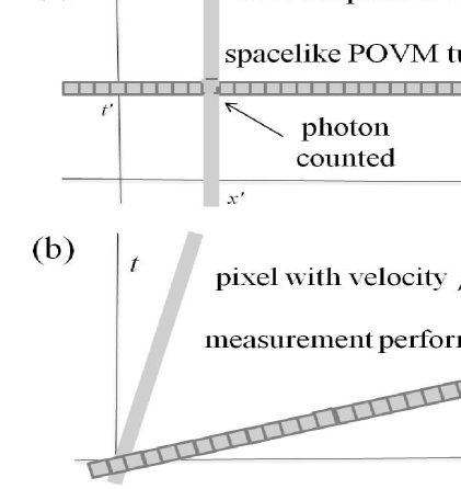
Figure 1: Inertial detectors. (a) Stationary spacelike POVM on $t=t^{\prime}$ and worldline of the pixel at $x=x^{\prime}$. The pixel at $x=x^{\prime}$ absorbs a single photon in the sketch but the array can count $0,\ 1,\ 2,$ .. photons. (b) Moving spacelike POVM with velocity $\beta$ on the hypersurface $t=\beta x$ and worldline $x=\beta t$ of one of its hyperpixels.

A spacelike POVM describing an array of accelerated detectors is sketched in Fig. 2. According to (4) each point on the array has a different acceleration $\alpha.$ This guarantees that the array is rigid in the sense that its ”$3$-geometry as seen from its own momentary rest frame is unchanged in the course of proper time” MMdelRay . The acceleration will dependent on penetration depth into the semiconductor but it is assumed that the photon is absorbed so these details are ignored. The solid and dashed lines in Fig. 2 represent surfaces of single accelerated devices traveling on the hyperbolic worldlines $x^{2}-t^{2}=a^{-2}\exp\left(2a\xi\right)$ in wedges I and II.

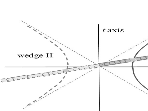
Figure 2: Rindler spacelike POVM on $\eta=\eta^{\prime}$ (gray boxes). The solid (dashed) line is the worldline of one of its hyperpixels in wedge I (II).

IV Photon number density and scalar product

This section starts with a review of the 4D photon counting operator. The Minkowski vacuum appears thermal to an accelerated observer and operators are useful for describing absorption and emission in this multiphoton state. For a paraxial beam with definite polarization and negligible transverse wave vectors the problem is effectively two dimensional and the 2D approximation will be used is the remainder of this paper for simplicity. In 2D a definite polarization photon field is mathematically equivalent to the zero mass Klein Gordon field. While the 2D approximation is problematic because of infrared divergences Coleman , it is a good model for explaining the Unruh effect Crispino .

The invariance of the indefinite scalar product follows from the continuity equation for four-current Hawking . For photons the four-current operator can be written in terms of the four-vector potential operator as follows HawtonMelde : In the Heisenberg picture the positive frequency part of the four-potential operator in the Lorentz gauge is

$$\widehat{A}^{\left(+\right)\mu}\left(t,\mathbf{x}\right)=\sum_{\lambda}\int_{-\infty}^{\infty}d^{3}k\frac{\exp\left(i\mathbf{k\cdot x}-i\left|\mathbf{k}\right|t\right)}{2\pi\left(4\pi\left|\mathbf{k}\right|\right)^{1/2}}e_{\lambda}^{\mu}\left(\mathbf{k}\right)\widehat{a}_{\lambda}\left(\mathbf{k}\right)$$ (7)

where $\widehat{a}_{\lambda}\left(\mathbf{k}\right)$ annihilates a photon with wave vector $\mathbf{k\ }$and polarization $\lambda$. Its negative frequency part is $\widehat{A}^{\left(-\right)\mu}=\widehat{A}^{\left(+\right)\mu\dagger}$. Contraction of (7) with the second rank electromagnetic force tensor operator

$$\widehat{F}^{\left(+\right)\mu\nu}=\partial^{\mu}\widehat{A}^{\left(+\right)\nu}-\partial^{\nu}\widehat{A}^{\left(+\right)\mu}$$ (8)

gives the covariant four-flux operator

$$\widehat{J}^{\mu}=i\widehat{F}^{\left(-\right)\mu\nu}\widehat{A}_{\nu}^{\left(+\right)}-i\widehat{A}_{\nu}^{\left(-\right)}\widehat{F}^{\left(+\right)\mu\nu}$$ (9)

that satisfies a continuity equation. Its $0^{th}$ component is the number density operator

$$\widehat{J}^{0}=i\widehat{\mathbf{E}}^{\left(-\right)}\cdot\widehat{\mathbf{A}}^{\left(+\right)}-i\widehat{\mathbf{A}}^{\left(-\right)}\cdot\widehat{\mathbf{E}}^{\left(+\right)}.$$ (10)

A field is a quantity defined at every point of spacetime so, mathematically, both $\widehat{A}$ and $\widehat{F}$ are field operators. Potential operators can be identified by their $\left|\mathbf{k}\right|^{-1/2}$ dependance while $\widehat{F}$ whose elements are components of the electric and magnetic field operators has terms proportional to $\left|\mathbf{k}\right|^{1/2}$.  The extra factor $\left|\mathbf{k}\right|$ comes from the time derivative in $\mathbf{E}=-\partial\mathbf{A}/\partial t$. For a plane wave with definite frequency the factor $\left|\mathbf{k}\right|^{1/2}$ from $\mathbf{E}$ compensates for the factor $\left|\mathbf{k}\right|^{-1/2}$ from $\mathbf{A}$ to give the frequency independent probability that characterizes number density.

Once $\Sigma$ has been selected a transformation can be made to the Coulomb gauge where photons are described by the transverse vector potential alone. In 2D $\widehat{A}^{\mu}$ then has a single component which for consistency with QFT will be called $\widehat{\phi}$. The electric field operator is $\widehat{E}=-\partial\widehat{\phi}/\partial t$. In a Minkowski plane wave expansion the positive frequency part of $\widehat{\phi}$ is

$$\widehat{\phi}^{\left(+\right)}\left(t,x\right)=\int_{-\infty}^{\infty}dku_{k,M}\left(t,x\right)\widehat{a}_{k,M}$$ (11)

where $u_{k,M}$ are the usual Minkowski plane waves given here by (21). The absorption density operator (10) then reduces to

$$\widehat{n}^{\left(+\right)}\left(t,x\right)=i\widehat{\phi}^{\left(-\right)}\overleftrightarrow{\partial}_{t}\widehat{\phi}^{\left(+\right)}$$ (12)

where $f\overleftrightarrow{\partial}_{t}g\equiv f\partial_{t}g-\left(\partial_{t}f\right)g$, while the emission density operator is

$$\widehat{n}^{\left(-\right)}\left(t,x\right)=i\widehat{\phi}^{\left(+\right)}\overleftrightarrow{\partial}_{t}\widehat{\phi}^{\left(-\right)}.$$ (13)

For an electromagnetic field initially in the state $\left|\psi\right\rangle$ the probability density to count a photon at $\left(t^{\prime},x^{\prime}\right)$ is HawtonPOVM

$$w_{1}^{\left(+\right)}\left(t^{\prime},x^{\prime}\right)=\left\langle\psi\left|\widehat{n}^{\left(+\right)}\left(t^{\prime},x^{\prime}\right)\right|\psi\right\rangle.$$ (14)

For $\left(t^{\prime},x^{\prime}\right)$ and $\left(t^{\prime\prime},x^{\prime\prime}\right)$ in different pixels the field operators commute and the two photon correlation function can be written as

$$w_{2}^{\left(+\right)}=\left\langle\psi\left|\widehat{n}^{\left(+\right)}\left(t^{\prime},x^{\prime}\right)\widehat{n}^{\left(+\right)}\left(t^{\prime\prime},x^{\prime\prime}\right)\right|\psi\right\rangle.$$ (15)

To make a connection between the number density operator and the invariant scalar product positive and negative frequency fields can be defined for a one photon state $\left|\psi\right\rangle$ as

$$\psi^{\left(+\right)}\left(t,x\right) =\int_{-\infty}^{\infty}dk\left\langle 0\left|\widehat{a}_{k}\right|\psi\right\rangle u_{k,M}\left(t,x\right),$$ (16)

$$\psi^{\left(-\right)}\left(t,x\right) =\int_{-\infty}^{\infty}dk\left\langle\psi\left|\widehat{a}_{k}^{\dagger}\right|0\right\rangle u_{k,M}^{\ast}\left(t,x\right),$$ (17)

$$\psi\left(t,x\right) =\psi^{\left(+\right)}\left(t,x\right)+\psi^{\left(-\right)}\left(t,x\right).$$ (18)

These fields are potential-like since they contain a factor $\left|\mathbf{k}\right|^{-1/2}$. The invariant indefinite scalar product evaluated on the hypersurface $t=t^{\prime}$ is

$$\left(\chi,\psi\right) =\int_{-\infty}^{\infty}dx\left[\left\langle\chi\left|\widehat{n}^{\left(+\right)}\left(t,x\right)\right|\psi\right\rangle+\left\langle\chi\left|\widehat{n}^{\left(-\right)}\left(t,x\right)\right|\psi\right\rangle\right]$$

$$=i\int_{-\infty}^{\infty}dx\chi^{\ast}\left(t,x\right)\overleftrightarrow{\partial}_{t}\psi\left(t,x\right).$$ (19)

Integration over $x$ using $\left(u_{k^{\prime\prime},M},u_{k^{\prime},M}\right)=\delta\left(k^{\prime}-k^{\prime\prime}\right)$ gives the $k$-space form of the scalar product

$$\left(\chi,\psi\right) =\int_{-\infty}^{\infty}\frac{dk}{2\left|k\right|}\left[\chi^{\left(+\right)\ast}\left(k\right)\psi^{\left(+\right)}\left(k\right)\right.$$

$$\left.-\chi^{\left(-\right)\ast}\left(k\right)\psi^{\left(-\right)}\left(k\right)\right].$$ (20)

Analogous expressions to (11) to (20) exist for wedge I and II Rindler coordinates.

V Plane waves

The positive frequency Minkowski plane waves are BirrellDavies

$$u_{k^{\prime},M}\left(t,x\right)=\frac{\exp\left[ik^{\prime}\left(x-\epsilon_{k^{\prime}}t\right)\right]}{\sqrt{4\pi\left|k^{\prime}\right|}}$$ (21)

where $\epsilon_{k}=k/\left|k\right|$ is the sign of the Minkowski wave vector so the frequency $\epsilon_{k}k$ is positive. The factor $\left(2\left|k^{\prime}\right|\right)^{1/2}$ in the denominator is needed to compensate for $\overleftrightarrow{\partial}_{t}$ in the invariant scalar product. Only positive frequency basis states will be written down explicitly but the negative frequency states are just their complex conjugates. The prime denotes a definite value while unprimed coordinates are variable. On any $t=t^{\prime}$ hypersurface substitution of (21) in (19) gives the indefinite orthonormality relations

$$\left(u_{k^{\prime\prime},M},u_{k^{\prime},M}\right) =\delta\left(k^{\prime}-k^{\prime\prime}\right),$$ (22)

$$\left(u_{k^{\prime\prime},M}^{\ast},u_{k^{\prime},M}^{\ast}\right) =-\delta\left(k^{\prime}-k^{\prime\prime}\right),$$

$$\left(u_{k^{\prime\prime},M}^{\ast},u_{k^{\prime},M}\right) =\left(u_{k^{\prime\prime},M},u_{k^{\prime},M}^{\ast}\right)=0.$$

In $k$-space the Minkowski plane wave with wave vector $k^{\prime}$ is

$$u_{k^{\prime},M}\left(k\right)=\sqrt{2\left|k\right|}\delta\left(k-k^{\prime}\right).$$ (23)

It differs from the probability amplitude $\left(u_{k,M},u_{k^{\prime},M}\right)$ by the factor $\sqrt{2\left|k\right|}$ needed to give the orthonormality relations (22) with the scalar product (20).

The positive frequency Rindler plane waves are

$$u_{K^{\prime},I}\left(\eta,\xi\right) =\frac{\exp\left[iK^{\prime}\left(\xi-\epsilon_{K^{\prime}}\eta\right)\right]}{\sqrt{4\pi\left|K^{\prime}\right|}}\text{ in I}$$ (24)

$$=0\text{ in II}$$

$$u_{K^{\prime},II}\left(\eta,\xi\right) =\frac{\exp\left[iK^{\prime}\left(\xi+\epsilon_{K^{\prime}}\eta\right)\right]}{\sqrt{4\pi\left|K^{\prime}\right|}}\text{ in II}$$

$$=0\text{ in I}$$

where $\epsilon_{K}=K/\left|K\right|$. Positive frequency is defined from the perspective of an inertial observer. The sign of the coefficient of $\eta$ is reversed in wedge II because according to (2) an inertial observer sees increasing Rindler time $\eta$ as decreasing Minkowski time $t$. This is the sign convention used in BirrellDavies ; Carroll . In either wedge an inertial observer sees $K^{\prime}>0$ as outward propagation and $K^{\prime}<0$ as inward propagation in Fig. 2. On $\eta=\eta^{\prime}$ the Rindler plane waves in either wedge satisfy orthonormality relations analogous to (22). Rindler plane waves in different wedges are orthogonal.

The Minkowski and Rindler plane waves are related though the Bogoliubov coefficients BirrellDavies that will be evaluated by substituting (21) and (24) in (19) and then substituting (3). This direct calculation that is the 2D version of Longhi was performed to better understand the relationship between the in and out waves and positive and negative frequencies, all of which are needed here to define the localized states. Since the scalar product is invariant $\left(u_{k,M},u_{K,I}\right)$ can be evaluated on any hypersurface. On $t^{\prime}=\eta^{\prime}=0$ where the Rindler POVM is instantaneously at rest

$$\alpha_{kK}^{I} =\left(u_{k,M},u_{K,I}\right)$$ (25)

$$=\int_{x_{0}}^{\infty}dx\frac{\left|K\right|/\left(ax\right)+\left|k\right|}{4\pi\sqrt{\left|kK\right|}}e^{-ikx}\left(ax\right)^{iK/a},$$

$$\beta_{kK}^{I} =\left(u_{k,M}^{\ast},u_{K,I}\right)$$

$$=\int_{x_{0}}^{\infty}dx\frac{\left|K\right|/\left(ax\right)-\left|k\right|}{4\pi\sqrt{\left|kK\right|}}e^{ikx}\left(ax\right)^{iK/a}.$$

The lower limit $x_{0}$ was introduced because the $\left|K\right|/x$ integral is undefined at $x=0.$ Using Mathematica to evaluate these integrals,

$$\alpha_{kK}^{I} =\frac{\sqrt{\left|K\right|}}{2\pi a\sqrt{\left|k\right|}}\left(\frac{\left|k\right|}{a}\right)^{-iK/a}\Gamma\left(iK/a\right)e^{\pi\left|K\right|/2a}\delta_{\epsilon_{K},\epsilon_{k}}$$ (26)

$$+F\left(K\right)\left(ax_{0}\right)^{iK},$$

$$\beta_{kK}^{I} =-\frac{\sqrt{\left|K\right|}}{2\pi a\sqrt{\left|k\right|}}\left(\frac{\left|k\right|}{a}\right)^{-iK/a}\Gamma\left(iK/a\right)e^{-\pi\left|K\right|/2a}\delta_{\epsilon_{K},\epsilon_{k}}$$

$$+F\left(K\right)\left(ax_{0}\right)^{iK}.$$

The factor $\delta_{\epsilon_{K},\epsilon_{k}}$ excludes antiparallel Minkowski and wedge I Rindler wave vectors. $\alpha_{kK}^{I}$ $\left(\beta_{kK}^{I}\right)$ is the amplitude for the positive (negative) frequency Minkowski plane wave components of a positive frequency Rindler plane wave in wedge I. The rest of the Bogoliubov coefficients in wedge I can be found using

$$\left(\phi,\psi\right)=-\left(\phi^{\ast},\psi^{\ast}\right)=\left(\psi,\phi\right)^{\ast}.$$ (27)

For negative frequency Rindler plane waves $\left(u_{k,M}^{\ast},u_{K,J}^{\ast}\right)=-\alpha_{kK}^{I}$ and $\left(u_{k,M},u_{K,J}^{\ast}\right)=-\beta_{kK}^{I}.$ If the positive frequency Minkowski plane waves are expanded in the Rindler basis the Bololiubov coefficients are $\left(u_{K,I},u_{k,M}\right)=\alpha_{kK}^{I\ast}$ and $\left(u_{K,I}^{\ast},u_{k,M}\right)=-\beta_{kK}^{I\ast}$. In wedge II, on $t=0$, $i\partial_{t}u_{K,II}=\left(\Omega/\left|x\right|\right)u_{K,II}$ and $u_{K,II}=\left|ax\right|^{iK}/\sqrt{4\pi\left|K\right|}$ so the Bogoliubov coefficients are of the form (25) but with $x\rightarrow\left|x\right|$. Evaluation of $\alpha_{kK}^{II}$ and $\beta_{kK}^{II}$ using Mathematica gives

$$\delta_{\epsilon_{K},\epsilon_{k}}\text{ in I}\rightarrow-\delta_{\epsilon_{-K},\epsilon_{k}}\text{ in II}$$ (28)

in (26).

In the Minkowski vacuum an inertial device can only emit but a negative frequency Minkowski plane wave describing emission has both positive and negative frequency Rindler plane wave components so an accelerated device can absorb photons from the Minkowski vacuum. The probability density for absorption is

$$\left|\beta_{kK}^{J}\right|^{2}=\frac{1}{2\pi a\left|k\right|\left(e^{2\pi\left|K\right|/a}-1\right)}.$$ (29)

The Minkowski vacuum is thermal with Unruh temperature $T_{U}=a/2\pi$. The state vector describing the Minkowski vacuum in Rindler coordinates can be deduced from the Bogoliubov transformation Crispino . Since (26) to (28) give $\left(u_{k,M}^{\ast},u_{K,I}+e^{-\pi\left|K\right|/a}u_{-K,II}^{\ast}\right)=0$ the normalized Unruh modes

$$U_{K,I} =\frac{u_{K,I}+e^{-\pi\left|K\right|/a}u_{-K,II}^{\ast}}{\sqrt{1-e^{-2\pi\left|K\right|/a}}},$$ (30)

$$U_{K,II} =\frac{u_{K,II}+e^{-\pi\left|K\right|/a}u_{-K,I}^{\ast}}{\sqrt{1-e^{-2\pi\left|K\right|/a}}},$$

are purely positive frequency Minkowski states. The field operator expanded in Rindler plane waves is

$$\widehat{\phi}=\sum_{J=I,II}\int_{-\infty}^{\infty}dK\left(u_{K,J}\widehat{b}_{K,J}+u_{K,J}^{\ast}\widehat{b}_{K,J}^{\dagger}\right)$$ (31)

where $\widehat{b}_{K,J}$ annihilates a photon with wave vector $K$ in wedge $J$. When transformed to Unruh modes

$$\widehat{\phi} =\int_{-\infty}^{\infty}dK\left[U_{K,I}\left(\frac{\widehat{b}_{K,I}-e^{-\pi\left|K\right|/a}\widehat{b}_{-K,II}^{\dagger}}{\sqrt{1-e^{-2\pi\left|K\right|/a}}}\right)\right.$$ (32)

$$\left.+U_{K,II}\left(\frac{\widehat{b}_{K,II}-e^{-\pi\left|K\right|/a}\widehat{b}_{-K,I}^{\dagger}}{\sqrt{1-e^{-2\pi\left|K\right|/a}}}\right)+H.c.\right]$$

where the coefficients of $U_{K,J}$ annihilate the Minkowski vacuum. To write an expression for the Minkowski vacuum state in Rindler coordinates the wave vectors can be made discrete using periodic boundary conditions on $x=-L/2$ and $L/2$ where $K_{j}=j2\pi/L$ and then taking the limit as $L\rightarrow\infty$ to regain the continuum of wave vectors. For discrete wave vectors the Minkowski vacuum in the Rindler plane wave basis is described by the state vector

$$\left|0_{M}\right\rangle=\prod_{j=-\infty}^{\infty}C_{j}\sum_{n_{K_{j}}=0}^{\infty}e^{-n_{j}\pi\left|K_{j}\right|/a}\left|n_{K_{j}},I\right\rangle\otimes\left|n_{-K_{j}},II\right\rangle$$ (33)

where $C_{j}=\sqrt{1-e^{-2\pi\left|K_{j}\right|/a}}$. The details are given in Crispino . Eq. (33) is a product over modes of sums over the number of correlated pairs $n_{j}$.

VI Localized states

The plane wave (21) has equal amplitude at all points in space at time $t$ and phase factor $\exp\left[ik^{\prime}\left(x-\epsilon_{k^{\prime}}t\right)\right]$ while a $\delta$-function localized state has equal amplitude for all wave vectors with a phase that determines its position. In this section the Minkowski and Rindler plane waves in spacetime will be converted to localized states in momentum space by interchanging the roles of momentum and position. The recipe is straightforward: Exchange position and wave vector by interchanging the arguments with the subscripts. Move the $\sqrt{2\left|k\right|}$ from the denominator to the numerator to allow for the difference in the form of the $x$-space and $k$-space scalar product. Change the sign of the $x$-term in the exponent and interchange primed with unprimed coordinates because $t^{\prime}$ and $x^{\prime}$ are the coordinates of a specific localization event. With this prescription the positive frequency Minkowski localized states on the $t=t^{\prime}$ hypersurface are

$$u_{x^{\prime},M}\left(k\right)=\frac{\sqrt{2\left|k\right|}\exp\left[-ik\left(x^{\prime}-\epsilon_{k}t^{\prime}\right)\right]}{\sqrt{2\pi}}$$ (34)

for $-\infty>k>\infty$. The probability amplitude for wave vector $k$ is

$$\left(u_{k,M},u_{x^{\prime},M}\right)=\frac{\exp\left[-ik\left(x^{\prime}-\epsilon_{k}t^{\prime}\right)\right]}{\sqrt{2\pi}}.$$ (35)

Since $\widehat{a}_{k}\left|0\right\rangle=\left|u_{k,M}\right\rangle$, $\left(u_{k,M},u_{x^{\prime},M}\right)=\left\langle 0\left|\widehat{a}_{k}\right|u_{x^{\prime},M}\right\rangle$ so the spacetime the field (16) describing the localized state at $\left(t^{\prime},x^{\prime}\right)$ is

$$u_{x^{\prime},M}\left(t,x\right)=\int_{-\infty}^{\infty}dk\frac{\exp\left[ik\left(x-x^{\prime}\right)-i\epsilon_{k}k\left(t-t^{\prime}\right)\right]}{2\pi\sqrt{2\left|k\right|}}.$$ (36)

At $t=t^{\prime}$ this can be integrated to give $u_{x^{\prime},M}=\sqrt{2\pi}\left|x-x^{\prime}\right|^{-1/2}$ which is clearly nonlocal.

The Minkowski localized states (34) are orthonormal. This can be verified by substitution in the $k$-space scalar product (20) to give

$$\left(u_{x^{\prime},M},u_{x^{\prime\prime},M}\right) =\delta\left(x^{\prime}-x^{\prime\prime}\right),$$ (37)

$$\left(u_{x^{\prime},M}^{\ast},u_{x^{\prime\prime},M}^{\ast}\right) =-\delta\left(x^{\prime}-x^{\prime\prime}\right),$$

$$\left(u_{x^{\prime},M},u_{x^{\prime\prime},M}^{\ast}\right) =0.$$

Following the same recipe the Rindler localized states on $\eta=\eta^{\prime}$ are

$$u_{\xi^{\prime},I}\left(K\right) =\frac{\sqrt{2\left|K\right|}\exp\left[-iK\left(\xi^{\prime}-\epsilon_{K}\eta^{\prime}\right)\right]}{\sqrt{2\pi}}\text{ in I}$$ (38)

$$=0\text{ in II}$$

$$u_{\xi^{\prime},II}\left(K\right) =\frac{\sqrt{2\left|K\right|}\exp\left[-iK\left(\xi^{\prime}+\epsilon_{K}\eta^{\prime}\right)\right]}{\sqrt{2\pi}}\text{ in II}$$

$$=0\text{ in I}$$

for $-\infty>K>\infty.$ With the definitions (38) the Rindler orthonormality relations on $\eta=\eta^{\prime}$ are

$$\left(u_{\xi^{\prime},J},u_{\xi^{\prime\prime},J}\right) =\delta\left(\xi^{\prime}-\xi^{\prime\prime}\right),$$ (39)

$$\left(u_{\xi^{\prime},J}^{\ast},u_{\xi^{\prime\prime},J}^{\ast}\right) =-\delta\left(\xi^{\prime}-\xi^{\prime\prime}\right),$$

$$\left(u_{\xi^{\prime},J},u_{\xi^{\prime\prime},J}^{\ast}\right) =0,$$

$$\left(u_{\xi^{\prime},I},u_{\xi^{\prime\prime},II}\right) =0,\ etc.$$

VI.1 Rindler localized state as seen by a Minkowski observer

In this subsection the probability amplitudes for the Rindler localized states will be calculated in the Minkowski localized basis. First a Rindler plane wave will be expanded in the Minkowski localized basis because this intermediate result will be needed later. Then the Rindler localized states will be transformed to the Minkowski localized basis. The transformation coefficients from $k$ to $K$-space are $\alpha_{kK}^{I}$ and $\beta_{kK}^{I}$ given by (26). The probability amplitudes for the wedge I positive frequency Rindler plane waves in the Minkowski localized basis are

$$\left(u_{x,M},u_{K,I}\right) =\int_{-\infty}^{\infty}dk\frac{\exp\left(ikx\right)}{\sqrt{2\pi}}\alpha_{kK}^{I},$$ (40)

$$\left(u_{x,M}^{\ast},u_{K,I}\right) =\int_{-\infty}^{\infty}dk\frac{\exp\left(-ikx\right)}{\sqrt{2\pi}}\beta_{kK}^{I}.$$

The $k$-integrals were evaluated analytically using Mathematica. If $x>0$

$$\left(u_{x,M},u_{K,I}\right) =\ \frac{\left(ax\right)^{iK/a}}{\sqrt{2\pi ax}}e^{2\pi\left|K\right|/a-\varepsilon\left|K\right|/a}g\left(K\right)+f\left(K\right),$$ (41)

$$\left(u_{x,M}^{\ast},u_{K,I}\right) =\frac{\left(ax\right)^{iK/a}}{\sqrt{2\pi ax}}i\epsilon_{K}g\left(K\right)-f\left(K\right),$$

while if $x<0$

$$\left(u_{x,M},u_{K,I}\right) =-i\frac{\left|ax\right|^{iK/a}}{\sqrt{2\pi ax}}\epsilon_{K}e^{\pi\left|K\right|/a}g\left(K\right)+f\left(K\right),$$ (42)

$$\left(u_{x,M}^{\ast},u_{K,I}\right) =\frac{\left|ax\right|^{iK/a}}{\sqrt{2\pi ax}}e^{\pi\left|K\right|/a}g\left(K\right)-f\left(K\right),$$

where

$$g\left(K\right) \equiv\frac{1}{2\pi}\left(-1\right)^{1/4}\epsilon_{K}\sqrt{\frac{\left|K\right|}{a}}$$ (43)

$$\times\Gamma\left(\frac{1}{2}-i\frac{K}{a}\right)\Gamma\left(i\frac{K}{a}\right)e^{-\pi\left|K\right|/a},$$

$$\left|g\left(K\right)\right|^{2}=\left(e^{4\pi\left|K\right|/a}-1\right)^{-1}.$$ (44)

The small constant $\varepsilon$ was introduced to give a convergent integral and a finite linewidth that makes a $\delta$-function peak visible in the graphs. The $f\left(K\right)$ term is the integral of the $F\left(K\right)$ term in (26). For $x_{0}\ll x$

$$f\left(K\right)=\frac{i\left(ax_{0}\right)^{iK/a}}{\sqrt{2\pi\left|K\right|/a}}.$$

The factor $g\left(K\right)$ suggests a temperature $T=a/4\pi$ which is half the Unruh temperature. However, the plane wave annihilation and creation operators are the usual ones so in the Minkowski vacuum a Rindler observer sees a thermal distribution of photon numbers characterized by the Unruh temperature. The factor $g\left(K\right)$ is the result of integration over $k$ taking into account the nonlocality of the fields. For $x>0$ the emission and absorption probabilities look like $T_{U}/2$ but for $x<0$ the emission and absorption probabilities are equal.

Expressions (41) and (42) are probability amplitudes for Rindler plane waves in the Minkowski localized basis. Using these probability amplitudes and $\left(u_{K,I},u_{\xi,I}\right)=\exp\left(-iK\xi\right)/\sqrt{2\pi}$ the transformation coefficients from wedge I Rindler localized states to Minkowski localized states can be written as

$$\alpha_{x\xi}^{I} =\left(u_{x,M},u_{\xi,I}\right)$$ (45)

$$=\int_{-\infty}^{\infty}dK\left(u_{x,M},u_{K,I}\right)\frac{\exp\left(-iK\xi\right)}{\sqrt{2\pi}},$$

$$\beta_{x\xi}^{I} =\left(u_{x,M}^{\ast},u_{\xi,I}\right)$$

$$=\int_{-\infty}^{\infty}dK\left(u_{x,M}^{\ast},u_{K,I}\right)\frac{\exp\left(-iK\xi\right)}{\sqrt{2\pi}}.$$

The localized state $u_{\xi,J}$ is seen as positive frequency by a Rindler observer while $\alpha_{x\xi}^{I}$ and $\beta_{x\xi}^{I}$ are the probability amplitudes for positive and negative frequency Minkowski localized states respectively. Using (27) the Minkowski amplitudes for the negative frequency Rindler localized states are $\left(u_{x,M},u_{\xi,I}^{\ast}\right)=-\beta_{x\xi}^{I}$ and $\left(u_{x,M}^{\ast},u_{\xi,I}^{\ast}\right)=-\alpha_{x\xi}^{I}$. The inverse transformation from Minkowski localized states to the Rindler basis is $\left(u_{\xi,I},u_{x,M}\right)=\alpha_{x\xi}^{I\ast}$, $\left(u_{\xi,I}^{\ast},u_{x,M}\right)=-\beta_{x\xi}^{I\ast}$, $\left(u_{\xi,I},u_{x,M}^{\ast}\right)=\beta_{x\xi}^{I\ast}$ and $\left(u_{\xi,I}^{\ast},u_{x,M}^{\ast}\right)=-\alpha_{x\xi}^{I\ast}$. In wedge II use of (28) in (40) gives $\alpha_{x\xi}^{II}=-\alpha_{\left|x\right|\xi}^{I}$ and $\beta_{x\xi}^{II}=-\beta_{\left|x\right|\xi}^{I}$.

The $K$-integral in (45) was evaluated numerically. The integral of the rapidly oscillating $f\left(K\right)$ term is zero. If the Minkowski observer were to see the Rindler localized states $u_{\xi,J}$ as exactly localized, all $K^{\prime}s$ should have equal weight and the graph of $\left|\left(u_{K,I},u_{x,M}\right)\right|$ should be flat while all the other $K$-integrands should be zero. Examination of Fig. 3 shows that these conditions are fulfilled except near $K=0$ where the probability amplitudes diverge as $\left|K\right|^{-1/2}$. The flat region does lead to a $\delta$-function and, without the thermal factor, $\alpha_{x\xi}^{I}$ would equal $\delta\left(\ln\left|ax\right|-a\xi\right)/\left|ax\right|^{1/2}$. The thermal peaks give an additional delocalized component to all the curves.

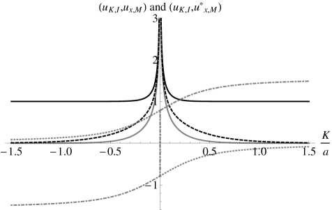
Figure 3: Thermal factors. The solid black and gray curves are plots of the absolute value of (41) and (42) respectively for $\left|ax\right|=1.$ The dotted and dash-dotted curves are $\arg\left(u_{K,I},u_{x,M}\right)$ and $\arg\left(u_{K,I},u_{x,M}^{\ast}\right)$.

The real functions $\left|ax\right|^{1/2}\alpha_{x\xi}^{I}$ and $\left|ax\right|^{1/2}\beta_{x\xi}^{I}$ are plotted in Fig. 4 as a function of $a\xi-\ln\left|ax\right|$. Both the peak in $\alpha_{x\xi}^{I}$ for $x>0$ and a delocalized contribution to all the curves are evident. As seen by an inertial observer a positive frequency Rindler localized state has a wedge I positive frequency peak at the correct position, but it has additional positive and negative frequency delocalized parts that are largest in wedge II.

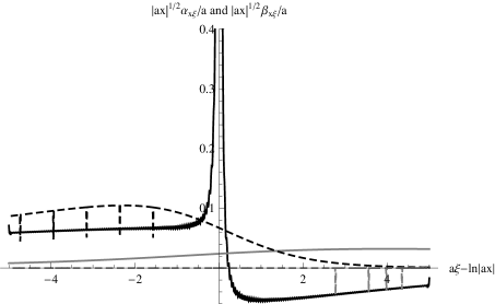
Figure 4: Real functions $\left|ax\right|^{1/2}\alpha_{x\xi}^{I}/a$ and $\left|ax\right|^{1/2}\beta_{x\xi}^{I}/a$ for $\varepsilon=0.01$ as a function of $a\xi-\ln\left|ax\right|$. The solid black and gray lines are $\alpha_{x\xi}^{I}$ and $\beta_{x\xi}^{I}$ in the wedge I where $x>0$ while the dashed line is $-\alpha_{x\xi}^{I}$ and $-\beta_{x\xi}^{I}$ in wedge II where $x<0.$ The hash marks are individual points where the integral did not converge.

In terms of the shifted Minkowski coordinate $X=x-a^{-1}$ the horizontal axis in Fig. 4 is

$$a\xi-\ln\left|1+aX\right|\simeq a\left(\xi-X\right)$$

for $\left|X\right|\ll a^{-1}$. For any definite value of $a$ the infinite $\alpha$ singularity at $X=a^{-1}$ exists and the equations and graphs in this section apply. The order in which the $X\rightarrow\infty$ and $a\rightarrow 0$ limit is taken matters: If the limit $a\rightarrow 0$ is taken before performing the calculation Rindler plane waves reduce to Minkowski plane waves and the graph in Fig. 4 should be replaced with $\delta$-function at $\xi=X$.

VII Discussion of localized states

The definition (34) leading to the orthonormality conditions (37) is based on Newton and Wigner’s (NW) seminal paper NW . NW exactly localized states, and indeed any state localized in a finite region, have paraxical properties: (i) the fields describing localized states are themselves nonlocal, (ii) they spread throughout space instantaneously, (iii) NW found no localized states for photons, and (iv) negative frequency states are needed for a complete basis and their QFT scalar products are negative. These properties are discussed below. A one-photon state and an inertial detector are considered for simplicity.

(i) For practical purposes the most important property of a localized basis is that the absolute square of the projection of the photon state vector onto the the localized states is the photon number probability density on $\Sigma$, $\left|\left(u_{x,M},\psi\right)\right|^{2}$ and $\left|\left(u_{x,M}^{\ast},\psi\right)\right|^{2}$. Here $\psi$ is the field (18) and $u_{x,M}$ is given by (34). Propagation of $\psi$ is not the subject of this paper, but the form of (11) and (21) ensures that the field will propagate at the speed of light. Inside the detector the damped field $E$ interacts with its atoms. The fact that a localized state is described by a nonlocal field such as (36) is not without observable consequences in photon counting experiments: Penetration depth and hence the time required for photon absorption are frequency dependent.

(ii) States that are localized in a finite region for an instant in time subsequently spread instantaneously Hegerfeldt . This causality paradox has a straigtforward interpretation: A localized state is a sum of counterpropagating waves whose nonlocal tails interfere destructively Prigogine . The exactly localized states are of this form as can be seen by inspection of (36). The field is nonlocal even on $t=t^{\prime}$ but the spacetime probability amplitude

$$\left(u_{t,x,M},u_{x^{\prime},t^{\prime},M}\right)=\frac{1}{2\pi}\int_{-\infty}^{\infty}dk\exp\left(ik\Delta x-i\epsilon_{k}k\Delta t\right).$$ (46)

with $\Delta x\equiv x-x^{\prime}$ and $\Delta t\equiv t-t^{\prime}$ is local. By inspection (46) is a sum of an $\epsilon_{k}=1$ wave propagating to the right and an $\epsilon_{k}=-1$ wave propagating to the left. Integration of (46) using $\lim_{\varepsilon\rightarrow 0}\left(\varepsilon\pm iz\right)^{-1}=\pi\delta\left(z\right)\mp i\mathcal{P}\left(1/z\right)$ where $\mathcal{P}$ is the principal value gives

$$\frac{1}{2}\left[\delta\left(\Delta x-\Delta t\right)+\delta\left(\Delta x+\Delta t\right)\right]$$

$$+\frac{i}{2\pi}\left[\mathcal{P}\left(\frac{1}{\Delta x-\Delta t}\right)-\mathcal{P}\left(\frac{1}{\Delta x+\Delta t}\right)\right].$$

For a localized state on the hypersurface $t=t^{\prime}$ the principal value terms interfere destructively leaving $\delta\left(x-x^{\prime}\right)$. At other times the nonlocal principal value terms are nonzero throughout space.

(iii) NW postulated that a localized state should be spherically symmetric NW . It can be proved that there is no photon position operator with commuting components that transforms like a vector Jordan78 . Because photon spin and orbital angular momentum cannot be separated, their localized states have definite total angular momentum and a vortex structure like twisted light AllenBarnettPadgett . When this is taken into account localized photon states and a photon position operator with commuting components can be constructed using the NW procedure HawtonBaylis . This photon position operator does not transform like a vector due to the extra term required to rotate its axis of symmetry, so the nonexistence proofs do not apply to it.

(iv) The indefinite scalar product (19) is positive for positive frequency basis states and negative for negative frequency states. Since positive frequency is associated with absorption and negative frequency with emission, the integral over $\Sigma$ gives the number of photons absorbed minus the number emitted. What matters is net absorption and a photon that is reemitted is not counted. This is reasonable since an atomic transition can be accompanied by an aborbed or emitted photon. Integration over time is needed to separate these processes and inertial and accelerated observers experience a different proper time. The invariance of the scalar product tells us that inertial and accelerated observers will agree on the number of atomic transitions and the probability of absorption minus the probability of emission but they will not agree on whether photons are emitted or absorbed.

Finally, the sum over histories gives a novel path-integral interpretation of the NW localized states that supports the interpretation that they describe a photon counting experiment: If the NW propagator is used in a relativistic calculation of the sum over paths crossing a intermediate spacelike hypersurface $\Sigma$ these paths must terminate on $\Sigma$ HalliwellOrtiz .

VIII Applications

In this section real devices and the Unruh effect will be discussed. Coincidence counting, single photon absorption events, and preparation of a one photon state will be considered.

If a device is prepared in its ground state initially it will contain no photons along its entire length. Photons are counted when they cross one of its surfaces travelling at speed $c$ and are absorbed within a penetration depth of a few wavelengths. (The speed of light $c$ has been reintroduced in this paragraph for clarity.) Calculation of the probability for this event requires flux (photon/s) but a spacelike hypersurface is required to define annihilation and creation operators and such a basis gives number density (photons/m). However, at normal incidence the Minkowski flux and number density are simply related through

$$\left\langle\psi\left|\widehat{J}^{1\left(+\right)}\left(t,x\right)\right|\psi\right\rangle=\pm c\left\langle\psi\left|\widehat{n}^{\left(+\right)}\left(t,x\right)\right|\psi\right\rangle$$ (47)

where the flux is positive (negative) for left to right (right to left) propagation. The localized basis states themselves do not contain information on the propagation direction but it will be assumed that the detector counts photons from only one direction and modes in the opposite direction are traced out. Eq. (47) gives the probability per unit time to absorb a photon in terms of the number density calculated using a basis of positive frequency localized states on a spacelike hypersurface.

In the vacuum state (33) for every wedge I photon with wave vector $K$ there is a wedge II photon with wave vector $-K$ (with the sign conventions used here). The zero photon term does not excite the detector. To first order in $e^{-\pi\left|K_{j}\right|/a}$ this leaves the one pair term with $C_{j}=1$ and this approximation will be considered first. Entanglement transfer from the vacuum to a pair of counteraccelerating Unruh-DeWitt detectors was studied in Reznik . Rindler observers in the causally disconnected wedges I and II cannot communicate but a Minkowski ”spectator” can receive signals from accelerated detectors in both wedges. Particle content measured by the two detectors each described by a single localized mode is predicted to be correlated DraganBruschi . Here a coincidence counting experiment performed by an inertial spectator with access to a pair of counteraccelerating photon counting detectors will be analyzed. For detectors that can absorb photons propagating from right to left described by the Rindler null coordinate $v\equiv\eta+\xi$ the $n_{K}=1$ term in (33) gives the probability amplitude for two photon absorption

$$\left\langle u_{v^{\prime},I}u_{v^{\prime\prime},II}|0_{M}\right\rangle =\int_{-\infty}^{0}dKe^{-\pi\left|K\right|/a}\frac{e^{iK\left(v^{\prime}-v^{\prime\prime}\right)}}{2\pi}$$

$$=\frac{1}{2\pi}\frac{1}{i\left(v^{\prime}-v^{\prime\prime}\right)+\pi/a}.$$ (48)

This describes Lorentzian spacetime correlations with linewidth $2\pi/a$. As $a\rightarrow 0$ the linewidth becomes infinite and as $a\rightarrow\infty$ $\left\langle u_{v^{\prime},I}u_{v^{\prime\prime},II}|0_{M}\right\rangle\rightarrow-\frac{1}{2}\delta\left(v^{\prime}-v^{\prime\prime}\right)-\frac{i}{2\pi}P\frac{1}{v^{\prime}-v^{\prime\prime}}$ where $P$ is the principle value. If positive and negative $K$ are included so (48) is a sum over counterpropagating waves $\left\langle u_{v^{\prime},I}u_{v^{\prime\prime},II}|0_{M}\right\rangle\rightarrow-\delta\left(v^{\prime}-v^{\prime\prime}\right)$ and the spacetime correlations are exact in the infinite acceleration limit.

If the photon in wedge II is not detected the probability density to count a photon in wedge I is the partial trace of the absolute square of (48) over $v^{\prime\prime}$ in wedge II equal to

$$\int_{-\infty}^{\infty}dv^{\prime\prime}\left|\left\langle u_{v^{\prime},I}u_{v^{\prime\prime},II}|0_{M}\right\rangle\right|^{2}=\frac{a}{4\pi^{2}}.$$ (49)

Eq (49) gives probability per unit Rindler time. The proper time interval is $d\tau=\pm\left(a/\alpha\right)d\eta$ where $\alpha=ae^{-a\xi}$ as given by (4). The probability per unit proper time for a detector with an absorbing surface at $\xi$ to count a photon is thus $\alpha/4\pi^{2}$.

Now imagine a that a single accelerated detector at $\xi^{\prime}$ in wedge I capable of absorbing photons propagating from right to left from the Minkowski vacuum clicks at Rindler time $\eta^{\prime}$. This process is most simply viewed from the instantaneous rest frame of the POVM where $t^{\prime}=\eta^{\prime}=0$. To first order the one pair term in (33) will collapse to a normalized one photon state described by the $K$-space and $\xi$-space Rindler probability amplitudes

$$\left(u_{K,II},\psi\right) =\left(\frac{\pi}{a}\right)^{1/2}e^{-\pi\left|K\right|/a}e^{-iK\xi^{\prime}},$$ (50)

$$\left(u_{\xi,II},\psi\right) =\frac{2\pi}{a^{3/2}}\left[\left(\xi-\xi^{\prime}\right)+i\frac{\pi}{a}\right]^{-1},$$

respectively. This is analogous to preparation of a one photon state using spontaneous parametric down conversion (SPDC). The Rindler field propagates causally after collapse at $t=\eta=0$. At Rindler time $\eta$ the peak of the pulse has propagated outward in wedge II to $\xi=\xi^{\prime}+\left|\eta\right|$ where $\eta<0$ since $t>0$. This is consistent with (48) if $\eta^{\prime}=0$ and $v=v^{\prime\prime}$ are substituted. In the Minkowski localized basis

$$\left(u_{x,M},\psi\right)=\int_{-\infty}^{\infty}dx\alpha_{x\xi}^{II}\left(u_{\xi,II},\psi\right).$$ (51)

The Minkowski field (18) with $\left\langle n_{k}\left|\widehat{a}_{k}\right|\psi\right\rangle=\left(u_{k,M},\psi\right)$ also propagates causally after collapse. According to Fig. 4 $\alpha_{x\xi}^{II}=-\alpha_{\left|x\right|\xi}^{I}$ has a delocalized component that is largest in wedge II. Thus the photon state prepared when a wedge I  accelerated detector counts a photon can lead to absorption by an accelerated detector in wedge II or by an inertial detector in either wedge.

The one pair term was considered first for clarity and to obtain analytic expressions, but all $n_{j}$ in (33) can be included by calculating the expectation values of the Rindler one and two photon density operators analogous to (14) and (15). The Rindler number density operators are

$$\widehat{n}_{J}^{\left(+\right)}\left(\xi\right)=i\widehat{\phi}_{J}^{\left(-\right)}\overleftrightarrow{\partial}_{\eta}\widehat{\phi}_{J}^{\left(+\right)}$$ (52)

where

$$\widehat{\phi}_{J}^{\left(+\right)}=\int_{-\infty}^{\infty}dKu_{K,J}\left(\eta,\xi\right)\widehat{b}_{K,J}$$ (53)

and $\widehat{\phi}_{J}^{\left(-\right)}=\widehat{\phi}_{J}^{\left(+\right)\dagger}$. For right to left propagation

$$w_{I}^{\left(+\right)} =\left\langle 0_{M}\left|\widehat{n}_{v^{\prime},I}^{\left(+\right)}\right|0_{M}\right\rangle$$

$$=\int_{-\infty}^{0}dK\left(e^{2\pi\left|K\right|/a}-1\right)^{-1}$$

This integral diverges at $\left|K\right|=0$ but there is a lower limit to the frequency response of any real detector. If a minimum frequency $\Omega_{0}=\left|K_{0}\right|$ is introduced the probability density per unit Rindler time for photon absorption is

$$w_{I}^{\left(+\right)}=-\frac{a}{\pi}\ln\left(1-e^{-2\pi\Omega_{0}/a}\right).$$ (54)

In the limit $2\pi\Omega_{0}/a\ll 1$ $w_{I}^{\left(+\right)}\cong-\left(a/\pi\right)\ln\left(2\pi\Omega_{0}/a\right)$ which diverges as $\Omega_{0}\rightarrow 0$. The two photon counting rate is

$$w_{I,II}^{\left(+\right)}=\left\langle 0_{M}\left|\widehat{n}_{v^{\prime},I}\widehat{n}_{v^{\prime\prime},II}\right|0_{M}\right\rangle.$$ (55)

To evaluate (55) consider the effect of annihilating a photon pair on $\left|0_{M}\right\rangle$. The $K$-factor of $\widehat{b}_{-K,II}\widehat{b}_{K,I}\left|0_{M}\right\rangle$ is

$$C_{K}\sum_{n_{K}=0}^{\infty}n_{K}e^{-n_{K}\pi\left|K\right|/a}\left|n_{K}-1,I\right\rangle\otimes\left|n_{-K}-1,II\right\rangle.$$ (56)

The probability for the $n$-pair term of this state combined with the $n$-pair term of $\left|0_{M}\right\rangle_{K}$ is $C_{K}^{2}e^{\pi\left|K\right|/a}n_{K}\left(e^{-2\pi\left|K\right|/a}\right)^{n}$. Defining $x=e^{-2\pi\left|K\right|/a}$ where $\sum_{n=0}^{\infty}nx^{n}=x/\left(1-x\right)^{2}$ and $C_{K}^{2}=1-x$, the sum over $n$ in (56) gives $\exp\left(\pi\left|K\right|/a\right)/\left[\exp\left(2\pi\left|K\right|/a\right)-1\right]$. There is also a $\widehat{b}_{K,I}\widehat{b}_{K^{\prime},II}\left|0_{M}\right\rangle$  term that gives the square of (54). For photons propagating from right to left

$$w_{I,II}^{\left(+\right)}=\left|\int_{-\infty}^{-\Omega_{0}}dK\frac{e^{\pi\left|K\right|/a-iK\left[\left(v^{\prime\prime}-v^{\prime}\right)\right]}}{2\pi\left(e^{2\pi\left|K\right|/a}-1\right)}\right|^{2}+w_{I}^{\left(+\right)}w_{II}^{\left(+\right)}.$$ (57)

The last term does not depend on the spacetime coordinates. The first term,

$$r_{I,II}=\left|\int_{-\infty}^{-\Omega_{0}}dK\frac{e^{\pi\left|K\right|/a-iK\left(v^{\prime\prime}-v^{\prime}\right)}}{2\pi\left(e^{2\pi\left|K\right|/a}-1\right)}\right|^{2},$$ (58)

is plotted in Fig. 5. The dotted line at the bottom is the first order approximation, equal to the absolute square of (48). The solid, dashed, dotdashed, and gray curves are $\Omega_{0}/a=.01$, $.02$, $.05$, and $.13$. The probability that an accelerated detector with cutoff frequency $\Omega_{0}$ will absorb a photon from the Minkowski vacuum is enhanced when all $n_{K}$ are included.

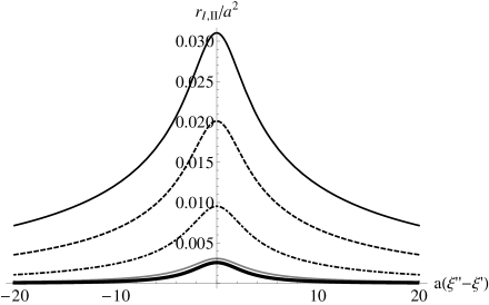
Figure 5: Coincidence counting rate$/a^{2}$ versus $a\left(v^{\prime\prime}-v^{\prime}\right)$.  The dotted line is the one pair term. The other lines are $r_{I,II}^{\left(+\right)}$ where the solid line is $\Omega_{0}/a=.01,$ the dashed line is $\Omega_{0}/a=.02$, the dotdashed line is $\Omega_{0}/a=.05$ and the gray line is $\Omega_{0}/a=.13$. $\Omega_{0}$ is the minimum (cutoff) frequency.

To obtain probability densities per unit proper time the constant $a$ should be replaced with the location dependent proper acceleration $\alpha=ae^{-a\xi}$ as in (49). Since $\exp\left(\pm iKd\eta\right)=\exp\left[\pm i\left(Ke^{-a\xi}\right)d\tau\right]$ in the instantaneous rest frame of the detector, the minimum frequency in units of proper time is $\omega_{0}=\Omega_{0}e^{-a\xi}$ so $\Omega_{0}/a=\omega_{0}/\alpha$ and (counts per unit Rindler time)$/a$ equals (counts per unit proper time)$/\alpha$ in Fig. 5 and all of the equation in this section. In SI units $a$ can be replaced with the acceleration frequency $a/c$ Crispino which has units $s^{-1}$ to give $\exp\left(-2\pi\Omega_{0}c/a\right)$ in Eqs. (54) to (58). An Unruh temperature $T_{U}=a\hbar/2\pi ck_{B}$ of $1K$ corresponds to an acceleration of $4\times 10^{21}ms^{-2}$ and an acceleration frequency $a/c=$ $2\times 10^{12}$ $s^{-1}$. For $c\Omega_{0}/a=.01$ a temperature of $1K$ requires a detector that can absorb photon with angular frequencies greater that $2\times 10^{10}$ $rad/s$.

IX Conclusion

In this paper bases of exactly localized Minkowski and Rindler states on spacelike hypersurfaces $\Sigma$ were used to construct POVMs for position measurements performed using small photon counting detectors. The transformation coefficients from Minkowski to Rindler localized states, $\alpha_{x\xi}^{J}$ and $\beta_{x\xi}^{J}$, were calculated and are plotted in Fig. 4. A photon field $\psi$ was defined whose positive frequency terms describe absorption of photons arriving from the past and whose negative frequency terms describe emission. The absolute squares of the indefinite scalar products of the positive frequency localized states with the field $\left|\left(u_{x,M},\psi\right)\right|^{2}$ and $\left|\left(u_{\xi,J},\psi\right)\right|^{2}$ are the probability densities for photon absorption by inertial and accelerated devices respectively. Using the relationship between photon density and flux this gives the probability that a photon will enter the detector and be absorbed. The exactly localized states are very convenient, largely because they are orthonormal and complete. While the states defining the POVM are exactly localized, this choice of basis does not impose limitations on the size of the photon counting detector or the form of the field incident on it.

These photon counting POVMs were applied to vacuum excitation of accelerated detectors (the Unruh effect). For right to left propagation described by the null Rindler coordinate $v=\eta+\xi$ the coincidence rate for absorption of correlated photons at $v^{\prime}$ in wedge I and $v^{\prime\prime}$ in wedge II was found to be a Lorentzian function of $v^{\prime}-v^{\prime\prime}$ with linewidth $2\pi/a$ where $a$ is the proper acceleration on $\xi=0$. If no measurement is performed in wedge II the wedge I probability per unit proper time to absorb a photon is proportional to the proper acceleration $\alpha=a\exp\left(-a\xi\right)$ where $\xi$ is the Rindler coordinate of the absorbing surface of the detector. Inclusion of numbers of photon pairs from $1$ to $\infty$ increases the coincidence counting density by a factor $10$ if the lowest frequency photon that can be absorbed by the detector is $\Omega_{0}=.01a$. If a photon is absorbed by an accelerated detector in wedge I the zero Rindler photon term is eliminated and the vacuum collapses to a one photon state plus higher order terms. This is consistent with the conclusion of Unruh and Wald UnruhWald : ”it seems as though the detector is excited by swallowing part of the vacuum fluctuation of the field in the region of spacetime containing the detector. This liberates the correlated fluctuation in a noncausally related region of the spacetime to become a real particle.” Here liberation of a photon is interpreted as collapse, analogous to preparation of a one photon state using SPDC. The photon state prepared in this way can, at least in principle, lead to absorption of a photon by an inertial detector.

Acknowledgements: The author thanks the Natural Sciences and Engineering Research Council for financial support.