Intermittency in relation with $1/f$ noise and stochastic differential equations

Abstract

One of the models of intermittency is on-off intermittency, arising due to time-dependent forcing of a bifurcation parameter through a bifurcation point. For on-off intermittency the power spectral density of the time-dependent deviation from the invariant subspace in a low frequency region exhibits $1/\sqrt{f}$ power-law noise. Here we investigate a mechanism of intermittency, similar to the on-off intermittency, occurring in nonlinear dynamical systems with invariant subspace. In contrast to the on-off intermittency, we consider the case where the transverse Lyapunov exponent is zero. We show that for such nonlinear dynamical systems the power spectral density of the deviation from the invariant subspace can have $1/f^{\beta}$ form in a wide range of frequencies. That is, such nonlinear systems exhibit $1/f$ noise. The connection with the stochastic differential equations generating $1/f^{\beta}$ noise is established and analyzed, as well.

The phrase “$1/f$ noise” refers to the well-known empirical fact that in many systems at low frequencies the noise spectrum exhibits an approximately $1/f$ shape. Generating mechanisms leading to $1/f^{\beta}$ noise are still an open question. Here we analyze nonlinear dynamical systems with invariant subspace having the transverse Lyapunov exponent equal to zero. In particular, we explore nonlinear maps having power-law dependence on the deviation from the invariant subspace. We demonstrate that such maps can generate signals exhibiting $1/f^{\beta}$ noise and intermittent behavior. In contrast to known mechanism of $1/f$ noise involving Pomeau-Manneville type maps, coefficients in the maps we consider are not static, similarly as in the maps describing on-off intermittency. We relate the nonlinear dynamics described by proposed maps to $1/f$ noise models based on the nonlinear stochastic differential equations.

I Introduction

Intermittency is an apparently random alternation of a signal between a quiescent state and bursts of activity. In 1949, Batchelor and Townsend used the word intermittency to describe their observations of the patchiness of the fluctuating velocity field in a fully turbulent fluid.Batchelor and Townsend (1949) Many natural systems display intermittent behavior, for example, turbulent bursts in otherwise laminar fluid flows, sunspot activity, and reversals of the geomagnetic field. Well known models of intermittency include the three types introduced by Pomeau and Manneville,Pommeau and Manneville (1980) as well as crisis-induced intermittency.Grebogi et al. (1987) A different variety of intermittency was first reported when synchronized chaos in a coupled chaotic oscillator system undergoes the instability as the coupling constant is changed Fujisaka and Yamada (1985, 1986). This intermittency is now known as on-off intermittency. Platt, Spiegel, and Tresser (1993); Heagy, Platt, and Hammel (1994); Yamada, Fukushima, and Yazaki (1989); *Ott1994; *Lai1995; *Cenys1996; *Venkataramani1996; *Lai1996; *Lai1996a; *Fujisaka1998; *Harada1999; *Becker1999 On-off intermittency appears in nonlinear dynamical systems with invariant subspaces, where the dynamics restricted to the invariant subspace is chaotic and the system is close to a threshold of transverse stability of the subspace. The main difference of on-off intermittency from other types is in the mechanism of the origin: on-off intermittency relies on the time-dependent forcing of a bifurcation parameter through a bifurcation point; in Pomeau-Manneville intermittency and crisis-induced intermittency the parameters are static.

It is known that the on-off intermittency exhibits characteristic statistics: Yamada and Fujisaka (1986); *Yamada1990; *Fujisaka1987; *Fujisaka1993; *Suetani1999; *Fujisaka2000; *Fujisaka1997; *Miyazaki2000 (i) the probability density function (PDF) of the magnitude of deviation $\rho$ from the invariant subspace obeys the asymptotic power-law, $\rho^{-1+\eta}$, with a small positive exponent $\eta$, (ii) the power spectral density (PSD) of the time series $\{\rho(t)\}$ in a low-frequency region exhibits a power-law $1/\sqrt{f}$ dependence, and (iii) given an appropriately small threshold $\rho_{\mathrm{th}}$, the PDF of the laminar duration $\tau$ takes an asymptotic form $\tau^{-3/2}$ in a certain wide range of $\tau$. Platt, Spiegel, and Tresser (1993); Heagy, Platt, and Hammel (1994) Since on-off intermittency generates signals having $f^{-\beta}$ PSD with $\beta=1/2$, the question arises whether a mechanism of intermittency, similar to the on-off intermittency, can yield signals having other values of the exponent $\beta$ of PSD, in particular $\beta=1$. The purpose of this paper is to investigate this question.

Signals having the PSD at low frequencies $f$ of the form $S(f)\sim 1/f^{\beta}$ with $\beta$ close to $1$ are commonly referred to as “$1/f$ noise”, “$1/f$ fluctuations”, or “flicker noise.” Power-law distributions of spectra of signals with $0.5<\beta<1.5$, as well as scaling behavior in general, are ubiquitous in physics and in many other fields, including natural phenomena, human activities, traffics in computer networks and financial markets. Ward and Greenwood (2007); Weissman (1988); *Barabasi1999; *Gisiger2001; *Wong2003; *Wagenmakers2004; *Newman05; *Szabo2007; *Castellano2009; *Eliazar2009; *Eliazar2010; *Perc2010; *Werner2010; *Orden2010; *Kendal2011; *Torabi2011; *Diniz2011 Many models and theories of $1/f$ noise are not universal because of the assumptions specific to the problem under consideration. Recently, the nonlinear stochastic differential equations (SDEs) generating signals with $1/f$ noise were obtained in Refs. Kaulakys and Ruseckas, 2004; *Kaulakys2006 (see also recent papers Kaulakys and Alaburda (2009); Ruseckas and Kaulakys (2010)), starting from the point process model of $1/f$ noise. Kaulakys and Meškauskas (1998); *Kaulakys1999-1; *Kaulakys2000-1; *Kaulakys2000-2; *Gontis2004; *Kaulakys2005 Yet another model of $1/f$ noise involves a class of maps generating intermittent signals. It is possible to generate power-laws and $1/f$-noise from simple iterative maps by fine-tuning the parameters of the system at the edge of chaos Procaccia and Schuster (1983); Schuster (1988) where the sensitivity to initial conditions of the logistic map is a lot milder than in the chaotic regime: the Lyapunov exponent is zero and the sensitivity to changes in initial conditions follows a power-law. Costa et al. (1997) Manneville Manneville (1980) first showed that, tuned exactly, an iterative function can produce interesting behavior, power-laws and $1/f$ PSD. This mechanism for $1/f$ noise only works for type-II and type-III Pomeau-Manneville intermittency. Ben-Mizrachi et al. (1985) Intermittency as a mechanism of $1/f$ noise continues to attract attention. Laurson and Alava (2006); *Pando2007; *Shinkai2012

In this paper we consider a mechanism of intermittency, similar to the on-off intermittency, occurring in nonlinear dynamical systems with invariant subspace. In contrast to the on-off intermittency, we consider the case where the transverse Lyapunov exponent is zero. In recent years there is a growing interest in dynamical systems which are characterized by zero Lyapunov exponents, namely, which trajectories diverge nonexponentially. Zaslavsky (2007) Chaos in such dynamical systems is called weak chaos. By relating nonlinear dynamics with the $1/f$ noise model based on the nonlinear SDEs we show that for such nonlinear dynamical systems the power spectral density of the deviation from the invariant subspace can have $1/f^{\beta}$ form, i.e., $1/f$ noise in a wide range of frequencies. Thus a generalization of the on-off intermittency yields a new mechanism of $1/f^{\beta}$ noise with the asymptotically power-law PDF, originated from the commonly known phenomenon of the intermittency and weak chaos.

This paper is organized as follows: in Sec. II we propose a model of intermittency with zero transverse Lyapunov exponent and in Sec. III we present some examples of nonlinear maps exhibiting $1/f$ noise. To obtain analytical expressions of the PDF and PSD of the deviation from the invariant subspace, in Sec. IV we approximate discrete maps with SDEs. Section V summarizes our findings.

II Model of intermittency with zero transverse Lyapunov exponent

We consider two-dimensional maps having a skew product structure: Platt, Spiegel, and Tresser (1993)

$$x_{n+1}=F(x_{n})\,,\qquad y_{n+1}=G(x_{n},y_{n})\,.$$ (1)

The function $G$ has the property $G(x,0)=0$ and, thus, $y=0$ is the invariant subspace, while $y$ is the deviation form the invariant subspace. We assume that the dynamics $x_{n+1}=F(x_{n})$ in (1) restricted to the invariant subspace is chaotic. If the transverse Lyapunov exponent

$$\lambda_{\bot}=\lim_{N\rightarrow\infty}\frac{1}{N}\sum_{n=0}^{N-1}\ln\left|\frac{\partial G(x_{n},0)}{\partial y}\right|$$ (2)

along an orbit on the invariant subspace converges and is less than zero, then the invariant subspace is transversely stable with respect to this orbit.

In this article we consider the case when $\partial G(x,0)/\partial y=1$ and, consequently, the transverse Lyapunov exponent is zero. Furthermore, we will assume that the two terms with the lowest powers in the expansion of the function $G(x,y)$ in the power series of $y$ have the form

$$G(x,y)=y+g(x)y^{\eta}$$ (3)

with $\eta>1$. This form satisfies the condition $\partial G(x,0)/\partial y=1$. Particularly $\eta=2$, however, generally $\eta$ may be fractional, as well.

We will consider the case where the function $g(x)$ in Eq. (3) is not constant and can acquire both positive and negative values. Thus the expansion (3) leads to the the map for small values of $y_{n}$

$$y_{n+1}=y_{n}+z_{n}y_{n}^{\eta}\,,\qquad\eta>1\,,$$ (4)

where $z_{n}\equiv g(x_{n})$. It should be noted that when $\eta=1$, the map (4) becomes a multiplicative map $y_{n+1}=y_{n}(1+z_{n})$, which is essentially the same as the map considered in Ref. Heagy, Platt, and Hammel, 1994 for modeling of on-off intermittency. The map (4) is similar to Pomeau-Manneville map

$$y_{n+1}=y_{n}+ay_{n}^{\eta}\pmod{1}$$ (5)

on the unit interval with one marginally unstable fixed point located at $y=0$. Pommeau and Manneville (1980) The main difference from the map (4) is that in the Pomeau-Manneville map (5) the coefficient in the second term is static.

Let us consider the situation when $y_{n}>0$. If $z_{n}<0$ then the map (4) leads to the decrease of the deviation from the invariant subspace $y=0$, whereas for $z_{n}>0$ the deviation $y$ grows. In contrast to systems with nonzero transverse Lyapunov exponent, the growth or decrease of the deviation is not exponential. In fact, if the second term on the right-hand side of Eq. (4) is much smaller than the first and, consequently, Eq. (4) can be approximately replaced by the differential equation $dy/dt=y^{\eta}z$, the growth or decrease of the deviation $y$ can be described by a $q$-exponential function with $q=\eta$. The $q$-exponential function, used in the framework of nonextensive statistical mechanics, Tsallis (1988, 2009a, 2009b) is defined as

$$\exp_{q}(x)\equiv[1+(1-q)x]_{+}^{\frac{1}{1-q}}\,,$$ (6)

where $[x]_{+}\equiv\max\{x,0\}$. Thus, although the Lyapunov exponent is zero, the map can be characterized by a nonzero $q$-generalized Lyapunov coefficient.Costa et al. (1997); Tsallis (2009b)

If the average of the variable $z$ is positive, $\langle z\rangle>0$, and there is a global mechanism of reinjection, the map (4) leads to the intermittent behavior. As in on-off intermittency, the intermittent behavior appears due to the time-dependent forcing of a bifurcation parameter through a bifurcation point $z=0$, thus the behavior described by map (4) can be considered as a kind of on-off intermittency. However, on-off intermittency is usually investigated in dynamical systems with nonzero transverse Lyapunov exponent.

For small durations of the laminar phase, one can approximate the map (4) replacing $y_{n}$ in the second term on the right hand side with initial value $y_{0}$. In this case Eq. (4) describes a random walk with drift. Since the average displacement due to the diffusion grows as $\sqrt{t}$ and the displacement due to drift term is proportional to $t$, for small enough durations $t$ the diffusion is more important than the drift. It is known that for the unbiased random walk the distribution of the first return times has the power-law exponent $-3/2$. Redner (2001) Therefore, for small enough durations $t$ one can expect to observe the power-law form, $t^{-3/2}$, of the PDF of the laminar phase durations, the same as in on-off intermittency.

The first two terms in the expansion (3) do not allow to determine uniquely the PDF of the deviation $y$. In order to determine PDF of $y$ and PSD of the series $\{y_{n}\}$, we need to take into account more terms in the expansion of the function $G(x,y)$ in the power series of $y$. One of the possibilities that we will consider is for the third term in the expansion to be equal to $\gamma y^{2\eta-1}$ (note, that $2\eta-1>\eta$ when $\eta>1$), leading to the map

$$y_{n+1}=y_{n}+z_{n}y_{n}^{\eta}+\gamma y_{n}^{2\eta-1}\,.$$ (7)

Particularly, for $\eta=2$, $2\eta-1=3$ and Eqs. (3) and (7) display simple Taylor expansions. Note, that a mechanism of reinjection operates at large values of $y$ and does not change Eq. (7), written for small values of $y$ close to the inveriant subspace.

II.1 $q$-exponential transformation of random walk

Another example of the function $G(x,y)$ having the expansion in the power series of $y$ as in Eq. (4) can be obtained according to the following consideration: In Ref. Heagy, Platt, and Hammel, 1994 a map of the form

$$y_{n+1}=w_{n}y_{n}$$ (8)

was considered as a model of on-off intermittency. In the log domain this map transforms to

$$s_{n+1}=s_{n}+z_{n}\,,$$ (9)

where $s_{n}=\ln y_{n}$ and $z_{n}=\ln w_{n}$. The critical condition for the onset of on-off intermittency is the condition for unbiased random walk, $\langle z\rangle=0$. One of the reasons for intermittent behavior is highly non-linear relation $y_{n}=e^{s_{n}}$ between $s_{n}$ and $y_{n}$. We can expect intermittent behavior also using other nonlinear functions instead of the exponential function. One of the generalizations of the exponential function, which corresponds to the differential equation $dy/ds=y$, is the $q$-exponential function (6) obeying the equation $dy/ds=y^{\eta}$. Thus, instead of $y_{n}=e^{s_{n}}$ we will consider a relation $y_{n}=\exp_{\eta}(s_{n})$, leading to a map of the form

$$y_{n+1}=\exp_{\eta}(\ln_{\eta}(y_{n})+z_{n})=(y_{n}^{1-\eta}+(1-\eta)z_{n})^{\frac{1}{1-\eta}}\,,$$ (10)

where the $q$-logarithm, defined as Tsallis (2009a)

$$\ln_{q}(x)=\frac{x^{1-q}-1}{1-q},$$ (11)

is a function inverse to $q$-exponential function. Expanding the map (10) in power series of $y$ we get Eq. (4).

The $q$-exponential function $\exp_{\eta}(s_{n})$ tends to infinity as $s_{n}$ approaches $1/(\eta-1)$ and the variable $y_{n}=\exp_{\eta}(s_{n})$ can be introduced only when $s_{n}$ does not reach $1/(\eta-1)$. This can be achieved by modifying the map (9) for the values of $s_{n}$ close to $1/(\eta-1)$ in order to avoid reaching this value. The modification of the map (9) changes also the map (10) for large values of $y_{n}$, not allowing for the value of the expression $y_{n}^{1-\eta}+(1-\eta)z_{n}$ to become zero.

III Numerical examples

In this Section we present some examples of the map (1) with the function $G(x,y)$ whose behavior for small values of $y$ is described by Eq. (7) or Eq. (10). Let us consider the map (7) with $\eta=2$, $\gamma=0.5$ when the variable $z_{n}$ has the average $\langle z\rangle=5\times 10^{-5}$ and the variance $\langle(z-\langle z\rangle)^{2}\rangle=1$. The parameters of the map are chosen taking into account equations from Sec. IV. The chosen value of the average $\langle z\rangle$ is close to the critical value for the onset of intermittency $\langle z\rangle=0$ and is much smaller than the standard deviation of the variable $z_{n}$. As a mechanism of reinjection we use a reflection at $y=0.5$, leading to the map

$$y_{n+1}=0.5-|y_{n}+z_{n}y_{n}^{2}+0.5y_{n}^{3}-0.5|\,.$$ (12)

As a map $x_{n+1}=F(x_{n})$ in Eq. (1) we take the chaotic driving by a tent map

$$x_{n+1}=\begin{cases}2x_{n}\,,&0\leq x_{n}\leq\frac{1}{2}\\ 2-2x_{n}\,,&\frac{1}{2}\leq x_{n}\leq 1.\end{cases}$$ (13)

The variable $z_{n}$ with given average $\langle z\rangle$ and variance $\langle(z-\langle z\rangle)^{2}\rangle$ can be obtained from $x_{n}$ using the equation

$$z_{n}=\sqrt{\frac{\langle(z-\langle z\rangle)^{2}\rangle}{\langle(x-\langle x\rangle)^{2}\rangle}}(x_{n}-\langle x\rangle)+\langle z\rangle\,.$$ (14)

For the tent map (13) the average and the variance are $\langle x\rangle=0.5$ and $\langle(x-\langle x\rangle)^{2}\rangle=1/12$, respectively.

Another example is when the variable $z_{n}$ acquires only two values $\pm\zeta$, with the probabilities $p_{+}$ and $p_{-}$, $p_{+}+p_{-}=1$. In this case the average and the variance of $z_{n}$ are given by the equations$\langle z\rangle=\zeta(p_{+}-p_{-})$ and $\langle(z-\langle z\rangle)^{2}\rangle=4\zeta^{2}p_{+}p_{-}$. Expressing the probabilities we get

$$p_{\pm}=\frac{1}{2}\pm\frac{\langle z\rangle}{2\sqrt{\langle(z-\langle z\rangle)^{2}\rangle+\langle z\rangle^{2}}}$$ (15)

and

$$\zeta=\sqrt{\langle(z-\langle z\rangle)^{2}\rangle+\langle z\rangle^{2}}\,.$$ (16)

In particular, if $\langle(z-\langle z\rangle)^{2}\rangle=1$, $\langle z\rangle=5\times 10^{-5}$ then $p_{+}\approx 0.500025$, $p_{-}\approx 0.499975$, $\zeta\approx 1.00000000125$. Such two-valued variable $z_{n}$ can be implemented by the following map:

$$y_{n+1}=\begin{cases}y_{n}-y_{n}^{2}\zeta+0.5y_{n}^{3}\,,&0\leqslant x_{n}\leqslant p_{-},\\ 0.5-|y_{n}+y_{n}^{2}\zeta+0.5y_{n}^{3}-0.5|\,,&p_{-}<x_{n}\leqslant 1.\end{cases}$$ (17)

Note, that also in the map (17) we use a reflection at $y=0.5$ as a mechanism of reinjection.

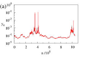
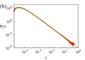
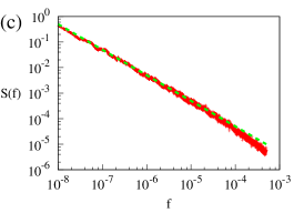
Figure 1: (Color online) (a) Time series of map described by Eqs. (12), (13), (14). (b) PDF of the variable $y$. The dashed (green) line is the analytical expression (29). (c) Power spectral density $S(f)$ of time series. The dashed (green) line shows the slope $1/f$. Parameters used are $\langle z\rangle=5\times 10^{-5}$ , $\langle(z-\langle z\rangle)^{2}\rangle=1$.

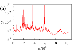
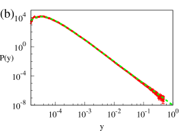
Figure 2: (Color online) (a) Time series of map described by Eqs. (13), (15)–(17). (b) PDF of the variable $y$. The dashed (green) line is the analytical expression (29). (c) Power spectral density $S(f)$ of time series. The dashed (green) line shows the slope $1/f$. Parameters used are the same as in Fig. 1.

The numerical results for maps described by Eqs. (12), (13), (14) and by Eqs. (13), (15)–(17) are shown in Fig. 1 and Fig. 2, respectively. We calculate the power spectral density directly, according to the definition, as the normalized squared modulus of the Fourier transform of the signal,

$$S(f)=\left\langle\frac{2}{N}\left|\sum_{n=1}^{N}y_{n}e^{-i2\pi fn}\right|^{2}\right\rangle,$$ (18)

where the angle brackets $\langle\cdot\rangle$ denote averaging over realizations. We used the time series $\{y_{n}\}$ of the length $N=10^{9}$ and averaged over $100$ realizations with randomly chosen initial value $y_{0}$.

From Fig. 1a and Fig. 2a we can see that these maps indeed lead to intermittent behavior, where the laminar phases are changed by bursts of activity corresponding to the large deviations of the variable $y$ from the average value. The laminar phases of the first map appear smoother than laminar phases of the second. The PDF of the variable $y$, shown in Fig. 1b and Fig. 2b, has in both cases a power-law form with the exponent $-3$ for larger values of $y$, whereas for small values of $y$ the PDF decreases exponentially. The PSD of the time series $\{y_{n}\}$, shown in Fig. 1c and Fig. 2c, has $1/f$ behavior for a wide range of frequencies. The $1/f$ interval in the PSD in Figs. 1c, 2c is $10^{-8}\lesssim f\lesssim 10^{-4}$.

For the map (10) we consider the case with $\eta=3$. To avoid reaching of the limiting value $s=1/(\eta-1)=0.5$ we modify the map (9) by introducing the reflection from the boundary $s_{n}=0.5$:

$$s_{n+1}=0.5-|s_{n}+z_{n}-0.5|\,.$$ (19)

Then the map (10) for the transformed variable $y_{n}=\exp_{\eta}(s_{n})$ takes the form

$$y_{n+1}=\frac{1}{\sqrt{\left|\frac{1}{y_{n}^{2}}-2z_{n}\right|}}\,.$$ (20)

For the variable $x_{n}$ we again use the tent map (13) and calculate $z_{n}$ according to Eq. (14) with the the average $\langle z\rangle=9\times 10^{-4}$ and the variance$\langle(z-\langle z\rangle)^{2}\rangle=1$.

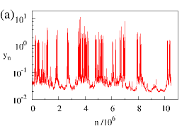
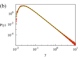
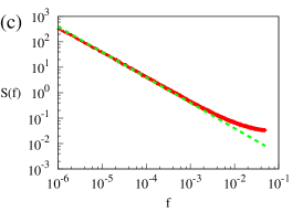
Figure 3: (Color online) (a) Time series of map described by Eqs. (13), (14), (20). (b) PDF of the variable $y$. The dashed (green) line is the analytical expression (29). (c) Power spectral density $S(f)$ of time series. The dashed (green) line shows the slope $1/f$. Parameters used are $\langle z\rangle=9\times 10^{-4}$, $\langle(z-\langle z\rangle)^{2}\rangle=1$.

The numerical results for the map described by Eqs. (13), (14), (20) are shown in Fig. 3. From Fig. 3a we can see that this map leads to the intermittent behavior. Due to larger average $\langle z\rangle$ and larger exponent $\eta$ the durations of laminar phases are shorter than in Figs. 1a, 2a. The PDF of the variable $y$, shown in Fig. 3b, has a power-law form with the exponent $-3$ for larger values of $y$, whereas for small values of $y$ the PDF decreases exponentially. The PSD of the time series $\{y_{n}\}$, shown in Fig. 3c, has $1/f$ behavior for a wide range of frequencies. The $1/f$ interval in the PSD is $10^{-6}\lesssim f\lesssim 10^{-3}$.

As the numerical examples show, both maps (7) and (10) for some values of the parameters can yield time series with $1/f$ PSD in a wide range of frequencies. In addition, the PDF of the deviation from the invariant subspace $y$ for these values of parameters has a power-law part with the exponent $-3$, in contrast to on-off intermittency where the exponent in the PDF is close to $-1$ and $1/\sqrt{f}$ PSD. The explanation of the observed behavior of PDF and PSD will be provided in the next Section.

IV Approximation of discrete maps by stochastic differential equations

To obtain analytical expressions for the PDF and PSD of the deviation $y$, we approximate the maps (7) and (10) by a SDE. To obtain the SDE corresponding to the map (7) we proceed as follows: we replace the variable $z_{n}$ by a random Gaussian variable having the same average and variance as $z_{n}$ and interpret Eq. (7) as Euler-Marujama approximation of a SDE. In this way we get the following SDE:

$$dy=\sigma^{2}\left(\eta-\frac{\nu}{2}+\frac{\eta-1}{2}\left(\frac{y_{\mathrm{min}}}{y}\right)^{\eta-1}\right)y^{2\eta-1}dt+\sigma y^{\eta}dW\,.$$ (21)

Here $W$ is a standard Wiener process (the Brownian motion) and the parameters $\sigma$, $y_{\mathrm{min}}$, and $\nu$ are given by the equations

$$\sigma = \sqrt{\langle(z-\langle z\rangle)^{2}\rangle}\,,$$ (22)

$$y_{\mathrm{min}} = \left[\frac{2\langle z\rangle}{(\eta-1)\langle(z-\langle z\rangle)^{2}\rangle}\right]^{\frac{1}{\eta-1}}\,,$$ (23)

$$\nu = 2\eta-\frac{2\gamma}{\langle(z-\langle z\rangle)^{2}\rangle}\,.$$ (24)

SDE approximating the map (10) can be obtained in the following way: we approximate a random walk described by Eq. (9) by a Brownian motion with constant drift $ds=adt+\sigma dW$, where $\sigma$ is given by Eq. (22) and $a=\langle z\rangle$. After transformation of the variable $s$ to the variable $y=\exp_{\eta}(s)$ we get a particular case of Eq. (21) with $\nu=\eta$, the other parameters $\sigma$ and $y_{\mathrm{min}}$ are given by Eqs. (22), (23). Thus, both maps (7) and (10) correspond to the same SDE (21). The SDE (21) has the same form as that considered in Refs. Kaulakys and Ruseckas, 2004; Kaulakys et al., 2006. It is possible to obtain the non-linear SDE of the form (21) starting from the agent-based herding model. Ruseckas, Kaulakys, and Gontis (2011) In Ref. Ruseckas and Kaulakys, 2011 modifications of these equations by introducing additional parameters are presented. These equations may generate signals with q-exponential and q-Gaussian distribution of the nonextensive statistical mechanics.

The approximation of the map (7) by the SDE (21) is valid when the value of $y$ is sufficiently small. The maximum value of $y$ can be determined from the condition that the second term in Eq. (7) should be much smaller than the first. We can estimate this condition as

$$y_{\mathrm{max}}^{\eta}\sqrt{\langle(z-\langle z\rangle)^{2}\rangle}\ll y_{\mathrm{max}}$$ (25)

giving

$$y_{\mathrm{max}}\lesssim\langle(z-\langle z\rangle)^{2}\rangle^{-\frac{1}{2(\eta-1)}}\,.$$ (26)

For the map (10) the approximation by the SDE (21) is valid as long as the variable $s_{n}$ is far from $1/(\eta-1)$ where the $q$-exponential function $\exp_{\eta}(s_{n})$ becomes infinite. Assuming that the presence of the limiting value $1/(\eta-1)$ does not influence the random walk (9) when the distance to this limiting value is larger than the standard deviation of $z_{n}$ (that is, $s_{n}<1/(\eta-1)-\sigma$) we can estimate the maximum value of $y$ as $y_{\mathrm{max}}\lesssim\exp_{\eta}(1/(\eta-1)-\sigma)$. This estimation coincides with Eq. (26).

Using Eqs. (23) and (26) we get the expression for the ratio $y_{\mathrm{max}}/y_{\mathrm{min}}$ :

$$\frac{y_{\mathrm{max}}}{y_{\mathrm{min}}}\lesssim\left[\frac{(\eta-1)\sqrt{\langle(z-\langle z\rangle)^{2}\rangle}}{2\langle z\rangle}\right]^{\frac{1}{\eta-1}}\,.$$ (27)

As it was shown in Refs. Kaulakys and Ruseckas, 2004; Kaulakys et al., 2006, the SDE (21) generates signals with power-law PSD in a wide range of frequencies when the variable $y$ can vary in a wide region, $y_{\mathrm{max}}\gg y_{\mathrm{min}}$. The condition $y_{\mathrm{max}}/y_{\mathrm{min}}\gg 1$ is obeyed when

$$\langle(z-\langle z\rangle)^{2}\rangle\gg\langle z\rangle^{2}\,,$$ (28)

that is, the standard deviation of the variable $z_{n}$ should be much larger than the average.

The SDE (21) leads to the steady state PDF

$$P_{0}(y)=\frac{(\eta-1)y_{\mathrm{min}}^{\nu-1}}{\Gamma\left(\frac{\nu-1}{\eta-1}\right)y^{\nu}}\exp\left[-\left(\frac{y_{\mathrm{min}}}{y}\right)^{\eta-1}\right]\,.$$ (29)

Thus, the parameter $\nu$ gives the exponent of the power-law part of the PDF and the parameter $y_{\mathrm{min}}$ gives the position of the exponential cut-off at small values of $y$. From Eq. (23) it follows that $y_{\mathrm{min}}$ grows with the growing average $\langle z\rangle$. As can be seen in Figs. 1b, 2b, 3b, there is a good agreement of the numerically obtained PDF with the analytical expression (29). Similarly as in the case of on-off intermittency we obtain PDF of the deviation from the invariant subspace having power-law form, however, the power exponent $\nu$ can assume values significantly different from $1$.

Numerical analysis, performed in Ref. Kaulakys and Alaburda, 2009 indicates that the stochastic variable $y$, described by a SDE similar to (21) exhibits intermittent behavior: there are peaks, bursts or extreme events, corresponding to the large deviations of the variable from the appropriate average value, separated by laminar phases with a wide range distribution of the laminar durations. The exponent $-3/2$ in the PDF of the interburst durations has been numerically obtained.

In Refs. Kaulakys and Ruseckas, 2004; Kaulakys et al., 2006 it was shown that SDE (21) generates signals with PSD having the form $S(f)\sim f^{-\beta}$ in a wide range of frequencies with the exponent

$$\beta=1+\frac{\nu-3}{2(\eta-1)}\,.$$ (30)

The connection of the PSD of the signal generated by SDE (21) with the behavior of the eigenvalues of the corresponding Fokker-Planck equation was analyzed in Ref. Ruseckas and Kaulakys, 2010. An additional argument based on scaling properties showing that PSD of the signal generated by SDE (21) has the power-law behavior in some range of frequencies we present in Appendix A. For the parameters used in Figs. 1, 2, 3, Eq. (30) gives $\beta=1$. Numerically obtained PSD shown in Figs. 1c, 2c, 3c confirms this prediction. Thus, as long as the approximation of the maps (7) or (10) by the SDE (21) is valid, the PSD of the time series $\{y_{n}\}$ exhibits a power-law behavior, including $1/f$ noise.

The range of frequencies where PSD has power-law behavior is limited by the minimum and maximum values $y_{\mathrm{min}}$ and $y_{\mathrm{max}}$. The limiting frequencies are estimated in Ref. Ruseckas and Kaulakys, 2010 and also in Appendix B. Using Eqs. (22), (23) and (26), we can write the range of frequencies (44) where the PSD has the power-law form as

$$\left(\frac{y_{\mathrm{min}}}{y_{\mathrm{max}}}\right)^{2(\eta-1)}\ll 2\pi f\ll 1\,.$$ (31)

If $y_{\mathrm{max}}/y_{\mathrm{min}}\gg 1$, this frequency range can span many orders of magnitude. However, this estimation of the frequency range is too broad and the numerical solution of Eq. (21) gives much narrower range. Nevertheless, Eq. (31) correctly reflects the following properties of the frequency region where PSD has $1/f^{\beta}$ dependence: the width of this frequency region increases with increase of the ratio between minimum and maximum values, $y_{\mathrm{min}}$ and $y_{\mathrm{max}}$, and with increase of the difference $\eta-1$. Ruseckas and Kaulakys (2010)

V Conclusions

We demonstrate that the nonlinear maps having invariant subspace and the expansion in the powers of the deviation from the invariant subspace having the form of Eq. (4) can generate signals with $1/f$ noise. In contrast to known mechanism of $1/f$ noise involving Pomeau-Manneville type maps, the parameter $z_{n}$ in the map Eq. (4) is not static. Another difference is that the exponent $\beta$ in the PSD, as Eq. (30) shows, depends on two parameters $\eta$ and $\nu$, thus $1/f^{\beta}$ noise can be obtained for various values of the exponent $\beta$.

The width of the frequency region where the PSD has $f^{-\beta}$ behavior is limited by the average value of the variable $z_{n}$: this width increases as $\langle z\rangle$ approaches the threshold value $\langle z\rangle=0$. In addition, the width of the power-law region in the PSD increases with increasing the difference $\eta-1$.

Appendix A Nonlinear stochastic differential equation generating signals with $1/f^{\beta}$ noise

Pure $1/f^{\beta}$ PSD is physically impossible because the total power would be infinity. Therefore we will consider signals with PSD having $1/f^{\beta}$ behavior only in some wide intermediate region of frequencies, $f_{\mathrm{min}}\ll f\ll f_{\mathrm{max}}$, whereas for small frequencies $f\ll f_{\mathrm{min}}$ PSD is bounded. We can obtain nonlinear SDE generating signals exhibiting $1/f$ noise using the following considerations. Wiener-Khintchine theorem relates PSD $S(f)$ to the autocorrelation function $C(t)$:

$$C(t)=\int_{0}^{+\infty}S(f)\cos(2\pi ft)dt\,.$$ (32)

If $S(f)\sim f^{-\beta}$ in a wide region of frequencies, then for the frequencies in this region the PSD has a scaling property

$$S(af)\sim a^{-\beta}S(f)$$ (33)

when the influence of the limiting frequencies $f_{\mathrm{min}}$ an $f_{\mathrm{max}}$ is neglected. From the Wiener-Khintchine theorem (32) it follows that the autocorrelation function has the scaling property

$$C(at)\sim a^{\beta-1}C(t)$$ (34)

in the time range $1/f_{\mathrm{max}}\ll t\ll 1/f_{\mathrm{min}}$. The autocorrelation function can be written as Ruseckas and Kaulakys (2010); Risken and Frank (1996); Gardiner (2004)

$$C(t)=\int dy\int dy^{\prime}\,yy^{\prime}P_{0}(y)P_{y}(y^{\prime},t|y,0)\,,$$ (35)

where $P_{0}(y)$ is the steady-state PDF and $P_{y}(y^{\prime},t|y,0)$ is the transition probability (the conditional probability that at time $t$ the signal has value $y^{\prime}$ with the condition that at time $t=0$ the signal had the value $y$). The transition probability can be obtained from the solution of the Fokker-Planck equation with the initial condition $P_{y}(y^{\prime},t|y,0)=\delta(y^{\prime}-y)$. The required property (34) can be obtained when the steady-state PDF has the power-law form

$$P_{0}(y)\sim y^{-\nu}$$ (36)

and the transition probability has the scaling property

$$P_{y}(ay^{\prime},t|ay,0)=a^{-1}P_{y}(y^{\prime},a^{2(\eta-1)}t|y,0)\,,$$ (37)

that is, change of the magnitude of the stochastic variable $y$ is equivalent to the change of time scale. In this case from Eq. (35) it follows that the autocorrelation function has the required property (34) with $\beta$ given by Eq. (30). In order to avoid the divergence of steady state PDF (36) the diffusion of stochastic variable $y$ should be restricted at least from the side of small values and, therefore, Eq. (36) holds only in some region of the variable $y$, $y_{\mathrm{min}}\ll y\ll y_{\mathrm{max}}$. When the diffusion of stochastic variable $y$ is restricted, Eq. (37) also cannot be exact. However, if the influence of the limiting values $y_{\mathrm{min}}$ and $y_{\mathrm{max}}$ can be neglected for time $t$ in some region $t_{\mathrm{min}}\ll t\ll t_{\mathrm{max}}$, we can expect that Eq. (34) approximately holds for this time region.

To get the required scaling (37) of the transition probability, the SDE should contain only powers of the stochastic variable $y$ and the coefficient in the noise term should be proportional to $y^{\eta}$. The drift term then is fixed by the requirement (36) for the steady-state PDF. Thus we consider SDE

$$dy=\sigma^{2}\left(\eta-\frac{1}{2}\nu\right)y^{2\eta-1}dt+\sigma y^{\eta}dW\,.$$ (38)

In order to obtain a stationary process and avoid the divergence of steady state PDF the diffusion of stochastic variable $y$ should be restricted or equation (38) should be modified. The simplest choice of the restriction is the reflective boundary conditions at $y=y_{\mathrm{min}}$ and $y=y_{\mathrm{max}}$. Exponentially restricted diffusion with the steady state PDF

$$P_{0}(y)\sim\frac{1}{y^{\nu}}\exp\left\{-\left(\frac{y_{\mathrm{min}}}{y}\right)^{m}-\left(\frac{y}{y_{\mathrm{max}}}\right)^{m}\right\}$$ (39)

is generated by the SDE

$$dy=\sigma^{2}\left[\eta-\frac{1}{2}\nu+\frac{m}{2}\left(\frac{y_{\mathrm{min}}^{m}}{y^{m}}-\frac{y^{m}}{y_{\mathrm{max}}^{m}}\right)\right]y^{2\eta-1}dt+\sigma y^{\eta}dW$$ (40)

obtained from Eq. (38) by introducing the additional terms.

Appendix B Estimation of the range of the frequencies where PSD has the power-law behavior

The presence of the restrictions at $y=y_{\mathrm{min}}$ and $y=y_{\mathrm{max}}$ makes the scaling (37) not exact and this limits the power-law part of the PSD to a finite range of frequencies $f_{\mathrm{min}}\ll f\ll f_{\mathrm{max}}$. Let us estimate the limiting frequencies. Taking into account the limiting values $y_{\mathrm{min}}$ and $y_{\mathrm{max}}$, Eq. (37) for the transition probability corresponding to SDE (38) becomes

$$P_{y}(ay^{\prime},t|ay,0;ay_{\mathrm{min}},ay_{\mathrm{max}})=\\ a^{-1}P_{y}(y^{\prime},a^{2(\eta-1)}t|y,0;y_{\mathrm{min}},y_{\mathrm{max}})\,.$$ (41)

The steady-state distribution $P_{0}(y;y_{\mathrm{min}},y_{\mathrm{max}})$ has the scaling property

$$P_{0}(ay;ay_{\mathrm{min}},ay_{\mathrm{max}})=a^{-1}P_{0}(y;y_{\mathrm{min}},y_{\mathrm{max}})\,.$$ (42)

Inserting Eqs. (41) and (42) into Eq. (35) we obtain

$$C(t;ay_{\mathrm{min}},ay_{\mathrm{max}})=a^{2}C(a^{2(\eta-1)}t,y_{\mathrm{min}},y_{\mathrm{max}})\,.$$ (43)

This equation means that time $t$ in the autocorrelation function should enter only in combinations with the limiting values, $y_{\mathrm{min}}t^{\frac{1}{2(\eta-1)}}$ and $y_{\mathrm{max}}t^{\frac{1}{2(\eta-1)}}$. We can expect that the influence of the limiting values can be neglected and Eq. (37) holds when the first combination is small and the second large, that is when time $t$ is in the interval $\sigma^{-2}y_{\mathrm{max}}^{2(1-\eta)}\ll t\ll\sigma^{-2}y_{\mathrm{min}}^{2(1-\eta)}$. Then, using Eq. (32) the frequency range where the PSD has $1/f^{\beta}$ behavior can be estimated as

$$\sigma^{2}y_{\mathrm{min}}^{2(\eta-1)}\ll 2\pi f\ll\sigma^{2}y_{\mathrm{max}}^{2(\eta-1)}\,.$$ (44)

References

- Batchelor and Townsend (1949) G. Batchelor and A. Townsend, Proc. R. Soc. London, Ser. A 199, 238 (1949).
- Pommeau and Manneville (1980) Y. Pommeau and P. Manneville, Commun. Math. Phys. 74, 189 (1980).
- Grebogi et al. (1987) C. Grebogi, E. Ott, F. Romeiras, and J. A. Yorke, Phys. Rev. A 36, 5365 (1987).
- Fujisaka and Yamada (1985) H. Fujisaka and T. Yamada, Prog. Theor. Phys. 74, 918 (1985).
- Fujisaka and Yamada (1986) H. Fujisaka and T. Yamada, Prog. Theor. Phys. 75, 1087 (1986).
- Platt, Spiegel, and Tresser (1993) N. Platt, E. A. Spiegel, and C. Tresser, Phys. Rev. Lett. 70, 279 (1993).
- Heagy, Platt, and Hammel (1994) J. F. Heagy, N. Platt, and S. M. Hammel, Phys. Rev. E 49, 1140 (1994).
- Yamada, Fukushima, and Yazaki (1989) T. Yamada, K. Fukushima, and T. Yazaki, Prog. Theor. Phys. Suppl. 99, 120 (1989).
- Ott and Sommerer (1994) E. Ott and J. C. Sommerer, Phys. Lett. A 188, 39 (1994).
- Lai and Grebogi (1995) Y.-C. Lai and C. Grebogi, Phys. Rev. E 52, R3313 (1995).
- Čenys et al. (1996) A. Čenys, A. Namajūnas, A. Tamaševičius, and T. Schneider, Phys. Lett. A 213, 259 (1996).
- Venkataramani et al. (1996) S. C. Venkataramani, J. T. M. Antonsen, E. Ott, and J. C. Sommerer, Physica D 96, 66 (1996).
- Lai (1996a) Y.-C. Lai, Phys. Rev. E 53, R4267 (1996a).
- Lai (1996b) Y.-C. Lai, Phys. Rev. E 54, 321 (1996b).
- Fujisaka et al. (1998) H. Fujisaka, K. Ouchi, H. Hata, B. Masaoka, and S. Miyazaki, Physica D 114, 237 (1998).
- Harada, Hata, and Fujisaka (1999) T. Harada, H. Hata, and H. Fujisaka, J. Phys. A 32, 1557 (1999).
- Becker et al. (1999) J. Becker, F. Rödelsperger, T. Weyrauch, H. Benner, W. Just, and A. Čenys, Phys. Rev. E 59, 1622 (1999).
- Yamada and Fujisaka (1986) T. Yamada and H. Fujisaka, Prog. Theor. Phys. 76, 582 (1986).
- Yamada and Fujisaka (1990) T. Yamada and H. Fujisaka, Prog. Theor. Phys. 84, 824 (1990).
- Fujisaka and Yamada (1987) H. Fujisaka and T. Yamada, Prog. Theor. Phys. 77, 1045 (1987).
- Fujisaka and Yamada (1993) H. Fujisaka and T. Yamada, Prog. Theor. Phys. 90, 529 (1993).
- Suetani and Horita (1999) H. Suetani and T. Horita, Phys. Rev. E 60, 422 (1999).
- Fujisaka, Suetani, and Watanabe (2000) H. Fujisaka, H. Suetani, and T. Watanabe, Prog. Theor. Phys. Suppl. 139, 70 (2000).
- Fujisaka, Matsushita, and Yamada (1997) H. Fujisaka, S. Matsushita, and T. Yamada, J. Phys. A 30, 5697 (1997).
- Miyazaki (2000) S. Miyazaki, J. Phys. Soc. Jpn. 69, 2719 (2000).
- Ward and Greenwood (2007) L. M. Ward and P. E. Greenwood, “1/f noise,” Scholarpedia 2, 1537 (2007).
- Weissman (1988) M. B. Weissman, Rev. Mod. Phys. 60, 537 (1988).
- Barabasi and Albert (1999) A. L. Barabasi and R. Albert, Science 286, 509 (1999).
- Gisiger (2001) T. Gisiger, Biol. Rev. 76, 161 (2001).
- Wong (2003) H. Wong, Microelectron. Reliab. 43, 585 (2003).
- Wagenmakers, Farrell, and Ratcliff (2004) E.-J. Wagenmakers, S. Farrell, and R. Ratcliff, Psychonomic Bull. Rev. 11, 579 (2004).
- Newman (2005) M. E. J. Newman, Contemp. Phys. 46, 323 (2005).
- Szabo and Fath (2007) G. Szabo and G. Fath, Phys. Rep. 446, 97 (2007).
- Castellano, Fortunato, and Loreto (2009) C. Castellano, S. Fortunato, and V. Loreto, Rev. Mod. Phys. 81, 591 (2009).
- Eliazar and Klafter (2009) I. E. Eliazar and J. Klafter, Proc. Natl. Acad. Sci. U.S.A. 106, 12251 (2009).
- Eliazar and Klafter (2010) I. E. Eliazar and J. Klafter, Phys. Rev. E 82, 021109 (2010).
- Perc and Szolnoki (2010) M. Perc and A. Szolnoki, Biosystems 99, 109 (2010).
- Werner (2010) G. Werner, Frontiers in Physiology 1, 1 (2010).
- Orden (2010) G. V. Orden, Medicina (Kaunas) 46, 581 (2010).
- Kendal and Jorgensen (2011) W. S. Kendal and B. Jorgensen, Phys. Rev. E 84, 066120 (2011).
- Torabi and Berg (2011) A. Torabi and S. S. Berg, Marine and Petroleum Geology 28, 1444 (2011).
- Diniz et al. (2011) A. Diniz, M. L. Wijnants, K. Torre, J. Barreiros, N. Crato, A. M. T. Bosman, F. Hasselman, R. F. Cox, G. C. V. Orden, and D. Deligni res, Human Movement Science 30, 889 (2011).
- Kaulakys and Ruseckas (2004) B. Kaulakys and J. Ruseckas, Phys. Rev. E 70, 020101(R) (2004).
- Kaulakys et al. (2006) B. Kaulakys, J. Ruseckas, V. Gontis, and M. Alaburda, Physica A 365, 217 (2006).
- Kaulakys and Alaburda (2009) B. Kaulakys and M. Alaburda, J. Stat. Mech. 2009, P02051 (2009).
- Ruseckas and Kaulakys (2010) J. Ruseckas and B. Kaulakys, Phys. Rev. E 81, 031105 (2010).
- Kaulakys and Meškauskas (1998) B. Kaulakys and T. Meškauskas, Phys. Rev. E 58, 7013 (1998).
- Kaulakys (1999) B. Kaulakys, Phys. Lett. A 257, 37 (1999).
- Kaulakys and Meškauskas (2000) B. Kaulakys and T. Meškauskas, Microel. Reliab. 40, 1781 (2000).
- Kaulakys (2000) B. Kaulakys, Microel. Reliab. 40, 1787 (2000).
- Gontis and Kaulakys (2004) V. Gontis and B. Kaulakys, Physica A 343, 505 (2004).
- Kaulakys, Gontis, and Alaburda (2005) B. Kaulakys, V. Gontis, and M. Alaburda, Phys. Rev. E 71, 051105 (2005).
- Procaccia and Schuster (1983) I. Procaccia and H. Schuster, Phys. Rev. A 28, 1210 (1983).
- Schuster (1988) H. G. Schuster, Deterministic Chaos (VCH, Weinheim, 1988).
- Costa et al. (1997) U. M. S. Costa, M. L. Lyra, A. R. Plastino, and C. Tsallis, Phys. Rev. E 56, 245 (1997).
- Manneville (1980) P. Manneville, J. Physique (Paris) 41, 1235 (1980).
- Ben-Mizrachi et al. (1985) A. Ben-Mizrachi, I. Procaccia, N. Rosenberg, A. Schmidt, and H. G. Schuster, Phys. Rev. A 31, 1830 (1985).
- Laurson and Alava (2006) L. Laurson and M. J. Alava, Phys. Rev. E 74, 066106 (2006).
- Pando L. and Doedel (2007) C. L. Pando L. and E. J. Doedel, Phys. Rev. E 75, 016213 (2007).
- Shinkai and Aizawa (2012) S. Shinkai and Y. Aizawa, J. Phys. Soc. Jpn. 81, 024009 (2012).
- Zaslavsky (2007) G. M. Zaslavsky, The Physics of Chaos in Hamiltonian Systems, 2nd ed. (Imperial College Pres, London, 2007).
- Tsallis (1988) C. Tsallis, J. Stat. Phys. 52, 479 (1988).
- Tsallis (2009a) C. Tsallis, Introduction to Nonextensive Statistical Mechanics: Approaching a Complex World (Springer, New York, 2009).
- Tsallis (2009b) C. Tsallis, Braz. J. Phys. 39, 337 (2009b).
- Redner (2001) S. Redner, A Guide to First-Passage Processes (Cambridge University Press, 2001).
- Ruseckas, Kaulakys, and Gontis (2011) J. Ruseckas, B. Kaulakys, and V. Gontis, EPL 96, 60007 (2011).
- Ruseckas and Kaulakys (2011) J. Ruseckas and B. Kaulakys, Phys. Rev. E 84, 051125 (2011).
- Risken and Frank (1996) H. Risken and T. Frank, The Fokker-Planck Equation: Methods of Solution and Applications (Springer, 1996).
- Gardiner (2004) C. W. Gardiner, Handbook of Stochastic Methods for Physics, Chemistry and the Natural Sciences (Springer-Verlag, Berlin, 2004).