Simplifying Generalized Belief Propagation on Redundant Region Graphs

Abstract

The cluster variation method has been developed into a general theoretical framework for treating short-range correlations in many-body systems after it was first proposed by Kikuchi in 1951. On the numerical side, a message-passing approach called generalized belief propagation (GBP) was proposed by Yedidia, Freeman and Weiss about a decade ago as a way of computing the minimal value of the cluster variational free energy and the marginal distributions of clusters of variables. However the GBP equations are often redundant, and it is quite a non-trivial task to make the GBP iteration converges to a fixed point. These drawbacks hinder the application of the GBP approach to finite-dimensional frustrated and disordered systems.

In this work we report an alternative and simple derivation of the GBP equations starting from the partition function expression. Based on this derivation we propose a natural and systematic way of removing the redundance of the GBP equations. We apply the simplified generalized belief propagation (SGBP) equations to the two-dimensional and the three-dimensional ferromagnetic Ising model and Edwards-Anderson spin glass model. The numerical results confirm that the SGBP message-passing approach is able to achieve satisfactory performance on these model systems. We also suggest that a subset of the SGBP equations can be neglected in the numerical iteration process without affecting the final results.

1 Introduction

Short loops are abundant in finite-dimensional ferromagnetic spin models and spin glass models. They cause complicated and strong local correlations in the systems. The accumulation and propagation of these local correlations then lead to long-range correlations and the emergence of various collective behaviors. The cluster variation method (CVM) is a general theoretical framework for treating local correlations in many-body statistical systems. The original idea of the cluster variation method was conceived by Professor Ryoichi Kikuchi (1919-2003) in $1951$ [1]. Since then CVM has been applied to many different types of systems and has been further developed and generalized [2, 3, 4, 5, 6]. The basic idea of CVM is to decompose the entropy of the whole system into the residual entropy contributions of various clusters of spin variables. After this decomposition, the true entropy of the system is approximated by the sum of residual entropy contributions from a properly chosen subset of spin clusters, see [2] or section 2.2 of [7] for a brief introduction.

The celebrated Bethe-Peierls tree approximation [8, 9, 10, 11] is an important limiting case of the cluster variation method. This tree approximation plays a central role in the mean-field theory of spin glasses [12, 13], and it is also underlying the widely used belief propagation (BP) message-passing algorithm in information science [14]. For various spin glass problems defined on finite-connectivity random graphs, due to the absence of short loops, the Bethe-Peierls approximation or its extended version (with the possibility of ergodicity breaking in the configuration space being considered) can give asymptotically exact results in the thermodynamic limit (see [13] for a comprehensive review). But the Bethe-Peierls approximation is inadequate in treating strong local correlations and therefore it performs poorly on finite-dimensional spin glass systems.

Considering more local correlations beyond the level of Bethe-Peierls approximation is conceptually easy within the CVM framework, but for strongly disordered and frustrated spin glass systems this task is practically quite challenging. There are two major issues: (a) How to construct a suitable variational marginal probability distribution for each chosen cluster of spin variables? (b) How to efficiently minimize the total Kikuchi cluster variational free energy, a complicated function of a large set of parameters? Yedidia and co-authors proposed in [15] a particular way of constructing cluster marginal probability distribution functions, and then they suggested a generalized belief propagation (GBP) message-passing approach to minimize the resulting Kikuchi variational free energy. This GBP message-passing approach outperforms the BP message-passing approach considerably in terms of numerical precision, but its widespread applications on finite-dimensional spin glass systems are still hindered by two important drawbacks: first, the GBP equations are often redundant; and second, it is quite a non-trivial task to make the GBP iteration converges to a fixed point.

In this work we understand the cluster marginal probability distribution functions of [15] from the viewpoint of the equilibrium partition function, and give an alternative and simple derivation of the GBP equations. Based on this derivation we propose a natural and systematic way of removing the redundance of the GBP equations. The resulting simplified generalized belief propagation (SGBP) equations are much more convenient for numerical implementation compared with the original GBP equations. We also point out that, for a given system, a subset of the SGBP equations can be safely ignored in the numerical iteration process. As redundance is minimized, the iteration process based on SGBP is much more easier to converge to a fixed point. We demonstrate the good performance of the SGBP equations by applying these equations to the two-dimensional (2D) and the three-dimensional (3D) ferromagnetic Ising model and Edwards-Anderson spin glass model.

The next section defines the general model system. The GBP equations are derived in section 3 starting from the partition function. These equations are then simplified in section 4. Some numerical results obtained by the SGBP equations are discussed in section 5. We conclude this work in section 6.

2 The general model system

We first define the general model system and briefly describe the region graph concept. A convenient expression for the partition function of the system is given.

2.1 Energy

Consider a system with $N$ vertices and $M$ two- or many-body interactions among the vertices. The indices of the vertices are denoted as $i,j,k,\ldots\in[1,N]$ and those of the interaction terms as $a,b,c,\ldots\in[1,M]$. Each vertex $i$ has a state $x_{i}$ which, for notational simplicity, is assumed to be a discrete scalar variable. A microscopic configuration of the system is denoted as $\underline{x}$, with $\underline{x}\equiv\{x_{1},\ldots,x_{i},\ldots,x_{N}\}$. The energy function has the following general form

$$H(\underline{x})=\sum\limits_{i=1}^{N}E_{i}(x_{i})+\sum\limits_{a=1}^{M}E_{a}(\underline{x}_{\partial a})\;.$$ (1)

In the above expression, $E_{i}(x_{i})$ and $E_{a}(\underline{x}_{\partial a})$ are, respectively, the self-energy of vertex $i$ and the energy of interaction $a$; $\partial a$ denotes the set of vertices involved in interaction $a$, and $\underline{x}_{\partial a}\equiv\{x_{i}|i\in\partial a\}$ is a microscopic sub-configuration for this particular set of vertices.

To give a concrete example of the general model system (1), let us mention the Edwards-Anderson (EA) spin glass system on a finite-dimensional regular lattice [16]. The vertices are then the lattice sites, each of them having a binary spin state ($x_{i}\in\{-1,+1\}$). There is a spin coupling interaction between each pair of nearest neighboring lattice sites. The energy of a given spin configuration is

$$H(\underline{x})=-\sum\limits_{i=1}^{N}h_{i}^{0}x_{i}-\sum\limits_{(i,j)}J_{ij}x_{i}x_{j}\;,$$ (2)

where $h_{i}^{0}$ is the external field on vertex (lattice site) $i$, and $(i,j)$ denotes a pair of nearest-neighboring vertices $i$ and $j$, with $J_{ij}$ being the coupling constant between them.

A conventional graphical representation for the general model system (1) is a bipartite graph of $N$ small circles (representing the vertices) and $M$ small squares (representing the interactions). Such a bipartite graph is referred to as a factor graph in the literature [17]. Each edge in the factor graph is between a small circle and a small square. If and only if a vertex $i$ is involved in an interaction $a$, then there will be an edge connecting the corresponding small circle and small square in the factor graph. As an example, figure 1 shows part of the factor graph for the EA model (2) on a periodic square lattice.

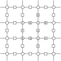
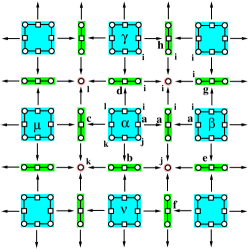
Figure 1: (a) Part of the factor graph for the Edwards-Anderson model on a square lattice (with periodic boundary condition on each side). Each small circle (such as $i$) denotes a vertex (lattice site); each small square (such as $a$) denotes a spin coupling interaction. An edge $(i,a)$ between a circle $i$ and a square $a$ means that vertex $i$ participates in interaction $a$. (b) Part of a redundant region graph for the factor graph of (a). Each square region (highlighted in cyan, such as $\alpha$ and $\beta$) contains four vertices and four interactions; each rod region (highlighted in green, such as $a$ and $b$) contains two vertices and one interaction; and each vertex region (highlighted in red, such as $i$ and $j$) contains only one vertex. A directed edge points from a parent region to a child region. Each vertex appears in $9$ regions (see the example of vertex $i$); and each interaction appears in $3$ regions (see the example of interaction $a$ between vertex $i$ and $j$). The counting number for a square region, a rod region and a vertex region is $c=1$, $c=-1$ and $c=1$, respectively.

2.2 Partition function and free energy

The partition function of system (1) has the sum-product form

$$Z(\beta)\equiv\sum_{\underline{x}}e^{-\beta H(\underline{x})}=\sum\limits_{\underline{x}}\prod\limits_{i=1}^{N}\psi_{i}(x_{i})\prod\limits_{a=1}^{M}\psi_{a}(\underline{x}_{\partial a})\;.$$ (3)

The inverse temperature $\beta\equiv\frac{1}{k_{B}T}$, with $T$ being the temperature (we shall set Boltzmann’s constant $k_{B}=1$ in the following discussions). The functions $\psi_{i}(x_{i})$ and $\psi_{a}(\underline{x}_{\partial a})$ are, respectively, the Boltzmann factor for the self-energy $E_{i}$ and the interaction energy $E_{a}$,

$$\psi_{i}(x_{i})\equiv e^{-\beta E_{i}(x_{i})}\;,\quad\quad\quad\psi_{a}(\underline{x}_{\partial a})\equiv e^{-\beta E_{a}(\underline{x}_{\partial a})}\;.$$ (4)

The equilibrium free energy $F(\beta)$ is related with the partition function $Z(\beta)$ as

$$F(\beta)\equiv-\frac{1}{\beta}\ln Z(\beta)\;.$$ (5)

Knowing the free energy $F$ as a function of inverse temperature $\beta$ and (if necessary) other environmental control parameters, we can then calculate all the other thermodynamic quantities such as the mean energy, the entropy, the mean value of $x_{i}$ for each vertex $i$. The free energy and the partition function therefore have fundamental importance in equilibrium statistical mechanics. But exactly computing the partition function (and the free energy) is an impossible task generically. Many numerical schemes have been developed over the years to obtain good approximate values for $Z(\beta)$ [4].

A well-known theoretical framework for performing approximation is Kikuchi’s cluster variation method [1, 2, 3, 5]. However, the variational problem of minimizing the Kikuchi cluster free energy is rather difficult to solve, especially for spin glass systems with quenched random parameters. Yedidia, Freeman, and Weiss [15] demonstrated that the minimal points of the Kikuchi variational free energy correspond to fixed points of a set of self-consistent generalized belief propagation (GBP) equations. Minimisation of the Kikuchi cluster free energy was therefore turned into the problem of constructing a fixed point for the GBP equations, which can be achieved through an iterative message-passing process on a region graph (see next subsection). Unfortunately, the GBP iterative process is still computationally demanding, especially when the underlying region graph are redundant.

In this work we will give an alterative and simple derivation of the GBP equations starting from the partition function (3). An advantage of this derivation is that it suggests a natural way of simplifying the GBP equations on redundant region graphs.

2.3 Region graph representation

The basic motivation of the region graph concept is to facilitate treatments of local correlations through distributing vertices into different overlapping groups, with each group containing a subset of vertices that are believed to be strongly correlated [1, 2, 15].

A region graph $R$ is a graph composed of regions and directed edges between pairs of regions [15]. The regions are generally denoted by Greek symbols. Each region $\gamma$ contains a subset of the vertices and a subset of the self-energies and interaction energies. If there is a directed edge from a region $\mu$ to another region $\nu$, denoted as $\mu\rightarrow\nu$, then $\nu$ must be contained in $\mu$ (namely all the vertices and all the energy contained in $\nu$ must also be contained in $\mu$). When the edge $\mu\rightarrow\nu$ is present, we say that $\mu$ is a parent of $\nu$ and $\nu$ a child of $\mu$. If there is a directed path from a region $\alpha$ to another region $\gamma$, we say that $\alpha$ is an ancestor of $\gamma$ and $\gamma$ a descendant of $\alpha$, and denote this ancestor–descendant relationship by $\alpha>\gamma$ and $\gamma<\alpha$. The notation $\alpha\geq\gamma$ ($\alpha\leq\gamma$) is understood as either $\alpha$ and $\gamma$ are identical to each other or $\alpha$ is an ancestor (descendant) of $\gamma$.

Figure 1 shows part of a region graph for the EA model of figure 1. There are three types of regions. Each square region contains four vertices and four interactions, and it is parent of four rod regions; each rod region contains two vertices and one interaction, and it is parent of two vertex regions; each vertex region contains a single vertex. In this particular example, for notational simplicity, each rod region is denoted by the index of the single interaction in it, and each vertex region is denoted by the index of the single vertex in it.

Each region $\gamma$ is assigned a counting number $c_{\gamma}$ [2], which is constructed recursively by

$$c_{\gamma}=1-\sum\limits_{\{\alpha\;:\;\alpha>\gamma\}}c_{\alpha}\;.$$ (6)

If a region $\alpha$ has no directed edges pointing to it, its counting number is $c_{\alpha}=1$. For a region $\mu$ with ancestors, it is obvious from the construction (6) that $c_{\mu}+\sum_{\gamma>\mu}c_{\gamma}\equiv 1$.

The vertices and energy terms of system (1) are clustered into various regions of $R$. This clustering, however, is not exclusive. A vertex and an energy term may be assigned to more than one region. To ensure that each energy term contributes only one Boltzmann factor to the partition function (3), the region graph $R$ is required to satisfy the following two constraints [15]: (1) For any vertex $i$, the induced subgraph $R_{i}$ (i.e., the region subgraph formed by all the regions containing $i$ and all the directed edges between pairs of these regions) is connected, and the sum of counting numbers within $R_{i}$ is unity:

$$\sum\limits_{\gamma\in R_{i}}c_{\gamma}=1\;;$$ (7)

and (2) for any interaction $a$, the induced subgraph $R_{a}$ (i.e., the region subgraph formed by all the regions containing $a$ and all the directed edges between pairs of these regions) is connected, and the sum of counting numbers within $R_{a}$ is unity:

$$\sum\limits_{\gamma\in R_{a}}c_{\gamma}=1\;.$$ (8)

Because of (7) and (8), the partition function can be expressed as

$$Z(\beta)=\sum\limits_{\underline{x}}\prod\limits_{\alpha\in R}\biggl{[}\prod_{i\in\alpha}\psi_{i}(x_{i})\prod_{a\in\alpha}\psi_{a}(\underline{x}_{\partial a})\biggr{]}^{c_{\alpha}}\;.$$ (9)

In our earlier work [18, 7], the expression (9) was the starting point for performing partition function expansion on the region graph $R$.

For each region $\alpha$ of a given region graph $R$, let us denote by $I_{\alpha}\equiv\{\gamma:\gamma\leq\alpha\}$ the set formed by region $\alpha$ and all its descendants, by $A_{\alpha}\equiv\{\gamma:\gamma>\alpha\}$ the set formed by all the regions ancestral to region $\alpha$, and by $B_{\alpha}$ the set that contains all the regions not belonging to set $I_{\alpha}$ but parental to at least one region of set $I_{\alpha}$ [7]. We refer to the set $I_{\alpha}$ as the interior of region $\alpha$ and set $B_{\alpha}$ as the boundary of region $\alpha$. As some examples, we show in figure 2 the interiors and boundaries of the square region $\alpha$, the rod region $a$ and the vertex region $i$ of the region graph of figure 1.

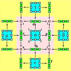
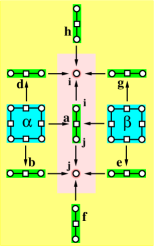
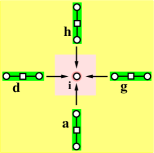
Figure 2: The interior and boundary for the square region $\alpha$ (a), the rod region $a$ (b), and the vertex region $i$ (c) of figure 1. The interior set $I_{\gamma}$ of any region $\gamma$ is marked by a pink-colored domain, while the boundary set $B_{\gamma}$ of region $\gamma$ is marked by a yellow-colored domain.

A region graph $R$ is referred to as non-redundant if the region subgraph $R_{i}$ induced by any vertex $i$ is a tree (containing no loops), otherwise $R$ is referred to as redundant [18, 7]. In a non-redundant region graph there is only one directed path from a region $\alpha$ to a descendant region $\gamma$, while in a redundant region graph there may exist multiple directed paths from an ancestral region $\alpha$ to a descendant region $\gamma$. The region graph shown in figure 1 is redundant, since there are two directed paths ($\alpha\rightarrow a\rightarrow i$ and $\alpha\rightarrow d\rightarrow i$) from the square region $\alpha$ to the vertex region $i$.

3 Generalized belief propagation (GBP) equations

We give an alternative derivation of the generalized belief propagation (GBP) equations [15] in this section. Let us introduce on each directed edge $\mu\rightarrow\nu$ of the region graph $R$ an arbitrary probability distribution function $m_{\mu\rightarrow\nu}(\underline{x}_{\nu})$, with the only constraints that this function is positive and is properly normalized, $\sum_{\underline{x}_{\nu}}m_{\mu\rightarrow\nu}(\underline{x}_{\nu})\equiv 1$. The function $m_{\mu\rightarrow\nu}(\underline{x}_{\nu})$ is a probability measure on the microscopic states $\underline{x}_{\nu}\equiv\{x_{i}|i\in\nu\}$ of region $\nu$. This measure is applied on $\nu$ by the parent region $\mu$. The probability $m_{\mu\rightarrow\nu}(\underline{x}_{\nu})$ can be regarded as a message from the parent region $\mu$ to the child region $\nu$ concerning the microscopic sub-configuration $\underline{x}_{\nu}$.

We observe that, for each directed edge $\mu\rightarrow\nu$,

$$\sum\limits_{\{\alpha\ :\ \mu\in B_{\alpha},\nu\in I_{\alpha}\}}c_{\alpha}=\sum\limits_{\alpha\geq\nu}c_{\alpha}-\sum\limits_{\alpha\geq\mu}c_{\alpha}=1-1=0\;.$$ (10)

This identity guarantees that the partition function (9) can be expressed as

$$Z(\beta)=\sum\limits_{\underline{x}}\prod\limits_{\alpha\in R}\biggl{[}\prod\limits_{i\in\alpha}\psi_{i}(x_{i})\prod\limits_{a\in\alpha}\psi_{a}(\underline{x}_{\partial a})\prod\limits_{\{\mu\rightarrow\nu\ :\ \mu\in B_{\alpha},\nu\in I_{\alpha}\}}m_{\mu\rightarrow\nu}(\underline{x}_{\nu})\biggr{]}^{c_{\alpha}}\;.$$ (11)

For each region $\alpha$ let us define a Boltzmann factor $z_{\alpha}$ as

$$z_{\alpha}=\sum\limits_{\underline{x}_{\alpha}}\prod\limits_{i\in\alpha}\psi_{i}(x_{i})\prod\limits_{a\in\alpha}\psi_{a}(\underline{x}_{\partial a})\prod\limits_{\{\mu\rightarrow\nu\ :\ \mu\in B_{\alpha},\nu\in I_{\alpha}\}}m_{\mu\rightarrow\nu}(\underline{x}_{\nu})\;.$$ (12)

Then the partition function can be re-written as

$$Z(\beta)=Z_{0}\times\sum\limits_{\underline{x}}\prod\limits_{\alpha\in R}\omega_{\alpha}(\underline{x}_{\alpha})^{c_{\alpha}}\;,$$ (13)

where $Z_{0}\equiv\prod\limits_{\alpha\in R}z_{\alpha}^{c_{\alpha}}$, and the weight $\omega_{\alpha}$ is defined as

$$\omega_{\alpha}(\underline{x}_{\alpha})\equiv\frac{1}{z_{\alpha}}\prod\limits_{i\in\alpha}\psi_{i}(x_{i})\prod\limits_{a\in\alpha}\psi_{a}(\underline{x}_{\partial a})\prod\limits_{\{\mu\rightarrow\nu\ :\ \mu\in B_{\alpha},\nu\in I_{\alpha}\}}m_{\mu\rightarrow\nu}(\underline{x}_{\nu})\;.$$ (14)

By exploiting the expression (13) we can write the free energy $F(\beta)$ as $F(\beta)=F_{0}+\Delta F$, with

$$F_{0}\equiv-\frac{1}{\beta}\ln Z_{0}=-\frac{1}{\beta}\sum\limits_{\alpha\in R}c_{\alpha}\ln\biggl{[}\sum\limits_{\underline{x}_{\alpha}}\prod\limits_{i\in\alpha}\psi_{i}(x_{i})\prod\limits_{a\in\alpha}\psi_{a}(\underline{x}_{\partial a})\prod\limits_{\{\mu\rightarrow\nu\ :\ \mu\in B_{\alpha},\nu\in I_{\alpha}\}}m_{\mu\rightarrow\nu}(\underline{x}_{\nu})\biggr{]}\;,$$ (15)

and correction contribution $\Delta F=-\frac{1}{\beta}\ln\bigl{[}\sum_{\underline{x}}\prod_{\alpha\in R}\omega_{\alpha}(\underline{x}_{\alpha})^{c_{\alpha}}\bigr{]}$.

Let us assume that $\Delta F$ can be safely neglected in comparison with $F_{0}$. Then the free energy can be approximated as $F(\beta)\approx F_{0}$. A rigorous justification of this approximation is absent, but it was shown in [18, 7] that, $\Delta F$ is the sum of correction contributions from looped region sub-graphs at least in the cases of non-redundant region graphs. We hope to return to this question in a future work.

The expression (15) for $F_{0}$ still contains all the auxiliary probability distribution functions. Naturally we require the free energy $F_{0}$ to be stationary with respect to the chosen set of probability functions $\{m_{\mu\rightarrow\nu}\}$. In other words, the first derivative of $F_{0}$ with respect to any $m_{\mu\rightarrow\nu}$ should be zero,

$$\frac{\delta F_{0}}{\delta m_{\mu\rightarrow\nu}}=0\;,\quad\quad\quad\forall(\mu\rightarrow\nu)\in G\;.$$ (16)

This condition is satisfied if we require the auxiliary functions to be chosen in such a way that, for each directed edge $\mu\rightarrow\nu$ of the region graph $G$,

$$\sum\limits_{\underline{x}_{\mu}\backslash\underline{x}_{\nu}}\omega_{\mu}(\underline{x}_{\mu})\ =\ \omega_{\nu}(\underline{x}_{\nu})\;.$$ (17)

Equation (17) ensures the consistency of the two marginal probability distributions $\omega_{\mu}(\underline{x}_{\mu})$ and $\omega_{\nu}(\underline{x}_{\nu})$ of each parent–child pair $(\mu,\nu)$. Equation (14) and Eq. (17) lead to the following generalized belief-propagation equation on each directed edge $\mu\rightarrow\nu$ of the region graph $R$:

$$\prod\limits_{\{\alpha\rightarrow\gamma\ :\ \alpha\in B_{\nu}\cap I_{\mu},\gamma\in I_{\nu}\}}m_{\alpha\rightarrow\gamma}(\underline{x}_{\gamma})=$$

$$\quad\quad\quad C\sum\limits_{\underline{x}_{\mu}\backslash\underline{x}_{\nu}}\prod\limits_{j\in\mu\backslash\nu}\psi_{j}(x_{j})\prod\limits_{b\in\mu\backslash\nu}\psi_{b}(\underline{x}_{\partial b})\prod\limits_{\{\eta\rightarrow\tau\ :\ \eta\in B_{\mu},\tau\in I_{\mu}\backslash I_{\nu}\}}m_{\eta\rightarrow\tau}(\underline{x}_{\tau})\;,$$ (18)

where $C$ is an adjustable constant to ensure that $m_{\mu\rightarrow\nu}(\underline{x}_{\nu})$ is properly normalized. The set of GBP equations (18) was first derived in [15] through a different approach.

If the region graph $R$ is non-redundant, then for each directed edge $\mu\rightarrow\nu$, $B_{\nu}\cap I_{\mu}=\{\mu\}$ and $\{\alpha\rightarrow\gamma:\alpha\in B_{\nu}\cap I_{\mu},\gamma\in I_{\nu}\}=\{\mu\rightarrow\nu\}$. Then equation (18) is simplified as

$$m_{\mu\rightarrow\nu}(\underline{x}_{\nu})=C\sum\limits_{\underline{x}_{\mu}\backslash\underline{x}_{\nu}}\prod\limits_{j\in\mu\backslash\nu}\psi_{j}(x_{j})\prod\limits_{b\in\mu\backslash\nu}\psi_{b}(\underline{x}_{\partial b})\prod\limits_{\{\eta\rightarrow\tau\ :\ \eta\in B_{\mu},\tau\in I_{\mu}\backslash I_{\nu}\}}m_{\eta\rightarrow\tau}(\underline{x}_{\tau})\;.$$ (19)

It can be shown that equation (19) is equivalent to the region graph belief propagation (rgBP) equation of [18, 7] obtained through partition function expansion.

If the region graph $R$ is redundant, then there are multiple directed paths between some pairs of regions. As a consequence, the consistency conditions (17) on some of the directed edges must be redundant. For example, because there are two directed paths $\alpha\rightarrow a\rightarrow i$ and $\alpha\rightarrow d\rightarrow i$ from the square region $\alpha$ to the vertex region $i$ in figure 2, then if the consistency conditions on the edges $\alpha\rightarrow a$, $\alpha\rightarrow d$ and $a\rightarrow i$ are all satisfied, the consistency condition on the edge $d\rightarrow i$ is satisfied automatically. For a redundant region graph, some of the consistency conditions (17) can therefore be dropped without affecting the final theoretical results. Consequently, some of the GBP equations (18) do not need to be considered.

4 Simplified GBP (SGBP) on a redundant region graph

In this paper we are interested in the case of the region graph $R$ being redundant. For example, figure 1 shows a redundant region graph for the 2D Edwards-Anderson model on a square lattice with period boundary conditions. In this region graph, the region subgraph $R_{i}$ induced by each vertex $i$ is not a tree. It contains nine regions and twelve directed edges, and loops exist in $R_{i}$ at the level of regions.

According to the definition (12), each boundary edge $(\mu\rightarrow\nu)$ of region $\alpha$ contributes a product term $m_{\mu\rightarrow\nu}(\underline{x}_{\nu})$ to the Boltzmann factor $z_{\alpha}$. As an example, consider the rod region $a$ of figure 2. Its Boltzmann factor $z_{a}$ is

$$z_{a} = \sum_{x_{i},x_{j}}\psi_{i}(x_{i})\psi_{j}(x_{j})\psi_{a}(x_{i},x_{j})m_{\alpha\rightarrow a}(x_{i},x_{j})m_{\beta\rightarrow a}(x_{i},x_{j})m_{h\rightarrow i}(x_{i})m_{f\rightarrow j}(x_{j})$$ (20)

$$\quad\quad\quad\quad\quad\quad\times m_{d\rightarrow i}(x_{i})m_{g\rightarrow i}(x_{i})m_{b\rightarrow j}(x_{j})m_{e\rightarrow j}(x_{j})\;.$$

Notice that the square region $\alpha$ and its two child rod regions $b$ and $d$ all send a message to region $a$ or its descendants, and these three messages are assumed to be mutually independent in the probability product form of equation (20). Similarly, the square region $\beta$ and its two child rod regions $e$ and $g$ contribute a product term of three probability messages to $z_{a}$. However, because the rod regions $b$ and $d$ are children of region $\alpha$, the probability message $m_{\alpha\rightarrow a}(x_{i},x_{j})$ already contains the effects of region $b$ and $d$ to region $a$. In other words, the probability distributions $m_{d\rightarrow i}(x_{i})$ and $m_{b\rightarrow j}(x_{j})$ very likely are strongly related to the probability distribution $m_{\alpha\rightarrow a}(x_{i},x_{j})$. Similarly, we expect the probability distributions $m_{g\rightarrow i}(x_{i})$ and $m_{e\rightarrow j}(x_{j})$ to be strongly related to the probability distribution $m_{\beta\rightarrow a}(x_{i},x_{j})$.

All such possibly strong dependence effects among the input probability distributions are completely neglected in (20) and in the more general expression (12). In this sense the redundance in the region graph structure causes redundance in the Boltzmann factor expressions (12), which in turn contributes at least part of the redundance in the set of GBP equations (18) and increases the complexity of numerical computations. The issue of removing the GBP redundance has been discussed by several recent studies [7, 6, 19, 20, 21].

We now propose a new way of removing redundance in the GBP equations. The basic idea is very simple: for a region $\nu$ in the boundary set $B_{\alpha}$ of region $\alpha$, the input probability messages from $\nu$ to the set $I_{\alpha}$ should be removed as many as possible if an ancestor of $\nu$ also belongs to the boundary set $B_{\alpha}$. Let us first discuss the ideal situation, namely the following equality is valid on each directed edge $\mu\rightarrow\nu$ of the region graph $R$:

$$\sum\limits_{\{\alpha\ :\ \mu\in B_{\alpha},\nu\in I_{\alpha},A_{\mu}\cap B_{\alpha}=\emptyset\}}c_{\alpha}=0\;,$$ (21)

where $A_{\mu}$ is the ancestor set of region $\mu$ as defined in section 2.3. The summation on the left-hand side of the above expression is over all the regions $\alpha$ satisfying the following conditions: (1) the boundary set $B_{\alpha}$ contains region $\mu$ but not any of the ancestors of $\mu$ ($A_{\mu}\cap B_{\alpha}=\emptyset$); and (2) the interior set $I_{\alpha}$ contains region $\nu$. As a simple example, let us mention that identity (21) is satisfied on each directed edge of the redundant region graph of figure 1. This particular region graph is therefore redundant and ‘ideal’.

If (21) holds on each directed edge $\mu\rightarrow\nu$, then the partition function expression (11) can be simplified as

$$Z(\beta)=\sum\limits_{\underline{x}}\prod\limits_{\alpha\in R}\biggl{[}\prod\limits_{i\in\alpha}\psi_{i}(x_{i})\prod\limits_{a\in\alpha}\psi_{a}(\underline{x}_{\partial a})\prod\limits_{\{\mu\rightarrow\nu\ :\ \mu\in B_{\alpha},\nu\in I_{\alpha},A_{\mu}\cap B_{\alpha}=\emptyset\}}m_{\mu\rightarrow\nu}(\underline{x}_{\nu})\biggr{]}^{c_{\alpha}}\;.$$ (22)

We can then define a simplified Boltzmann factor for region $\alpha$ as

$$\tilde{z}_{\alpha}\equiv\sum\limits_{\underline{x}_{\alpha}}\prod\limits_{i\in\alpha}\psi_{i}(x_{i})\prod\limits_{a\in\alpha}\psi_{a}(\underline{x}_{\partial a})\prod\limits_{\{\mu\rightarrow\nu\ :\ \mu\in B_{\alpha},\nu\in I_{\alpha},A_{\mu}\cap B_{\alpha}=\emptyset\}}m_{\mu\rightarrow\nu}(\underline{x}_{\nu})\;.$$ (23)

A simplified Boltzmann weight for region $\alpha$ is defined correspondingly:

$$\tilde{\omega}_{\alpha}(\underline{x}_{\alpha})\equiv\frac{1}{\tilde{z}_{\alpha}}\prod\limits_{i\in\alpha}\psi_{i}(x_{i})\prod\limits_{a\in\alpha}\psi_{a}(\underline{x}_{\partial a})\prod\limits_{\{\mu\rightarrow\nu\ :\ \mu\in B_{\alpha},\nu\in I_{\alpha},A_{\mu}\cap B_{\alpha}=\emptyset\}}m_{\mu\rightarrow\nu}(\underline{x}_{\nu})\;.$$ (24)

For the ideal redundant region graph of figure 1, the Boltzmann factor $\tilde{z}_{a}$ of the rod region $a$ is readily written down as (see figure 2)

$$\tilde{z}_{a}=\sum\limits_{x_{i},x_{j}}\psi_{i}(x_{i})\psi_{j}(x_{j})\psi_{a}(x_{i},x_{j})m_{\alpha\rightarrow a}(x_{i},x_{j})m_{\beta\rightarrow a}(x_{i},x_{j})m_{h\rightarrow i}(x_{i})m_{f\rightarrow j}(x_{j})\;,$$ (25)

which is much simpler than the expression (20).

The partition function is then expressed as

$$Z(\beta)=\tilde{Z}_{0}\times\sum\limits_{\underline{x}}\prod\limits_{\alpha}\tilde{\omega}_{\alpha}(\underline{x}_{\alpha})^{c_{\alpha}}\;,$$ (26)

where $\tilde{Z}_{0}\equiv\prod\limits_{\alpha}\tilde{z}_{\alpha}^{c_{\alpha}}$. A new approximate free energy $\tilde{F}_{0}$ is defined as

$$\tilde{F}_{0}\equiv-\frac{1}{\beta}\ln\tilde{Z}_{0}=-\frac{1}{\beta}\sum\limits_{\alpha\in R}c_{\alpha}\ln\biggl{[}\sum\limits_{\underline{x}_{\alpha}}\prod\limits_{i\in\alpha}\psi_{i}(x_{i})\prod\limits_{a\in\alpha}\psi_{a}(\underline{x}_{\partial a})\prod\limits_{\{\mu\rightarrow\nu\ :\ \mu\in B_{\alpha},\nu\in I_{\alpha},A_{\mu}\cap B_{\alpha}=\emptyset\}}m_{\mu\rightarrow\nu}(\underline{x}_{\nu})\biggr{]}\;.$$ (27)

Requiring $\tilde{F}_{0}$ to be stationary with respect to the set of auxiliary probability distributions $\{m_{\mu\rightarrow\nu}(\underline{x}_{\nu})\}$, the following set of simplified consistency conditions are obtained:

$$\sum\limits_{\underline{x}_{\mu}\backslash\underline{x}_{\nu}}\tilde{\omega}_{\mu}(\underline{x}_{\mu})\ =\ \tilde{\omega}_{\nu}(\underline{x}_{\nu})\;,\quad\quad\quad\forall(\mu\rightarrow\nu)\in R\;.$$ (28)

This consistency condition leads to the following simplified generalized belief propagation (SGBP) equation on each directed edge $\mu\rightarrow\nu$:

$$\prod\limits_{\{\alpha\rightarrow\gamma\ :\ \alpha\in B_{\nu}\cap I_{\mu},\gamma\in I_{\nu},A_{\alpha}\cap B_{\nu}=\emptyset\}}m_{\alpha\rightarrow\gamma}(\underline{x}_{\gamma})=$$

$$\quad\quad\quad\quad C\sum\limits_{\underline{x}_{\mu}\backslash\underline{x}_{\nu}}\prod\limits_{j\in\mu\backslash\nu}\psi_{j}(x_{j})\prod\limits_{b\in\mu\backslash\nu}\psi_{b}(\underline{x}_{\partial b})\prod\limits_{\{\eta\rightarrow\tau\ :\ \eta\in B_{\mu},\tau\in I_{\mu}\backslash I_{\nu},A_{\alpha}\cap B_{\mu}=\emptyset\}}m_{\eta\rightarrow\tau}(\underline{x}_{\tau})\;,$$ (29)

where $C$ is again an adjustable normalisation constant.

For a given spin glass model (1), it may be a relatively easy task to construct a redundant region graph that has the property (21) on each of its directed edges. The set of SGBP equations (29) can then be iterated on such an ‘ideal’ redundant region graph $R$, and the approximate free energy $\tilde{F}_{0}$ can be computed accordingly.

To be complete, let us also briefly discuss the ‘non-ideal’ case in which the identity (21) holds on some but not all of the directed edges. A simple solution would be to divide the directed edges into two classes (say $C_{I}$ and $C_{N}$), one ($C_{I}$) with the property (21) and the other one ($C_{N}$) with only the weaker property (10). For an edge $(\mu\rightarrow\nu)\in C_{I}$, the probability message $m_{\mu\rightarrow\nu}(\underline{x}_{\nu})$ is received by all the regions $\alpha$ in the set $\{\alpha:\mu\in B_{\alpha},\nu\in I_{\alpha},A_{\mu}\cap B_{\alpha}=\emptyset\}$. While for an edge $(\eta\rightarrow\tau)\in C_{N}$, we require the probability message $m_{\eta\rightarrow\tau}(\underline{x}_{\tau})$ to be received by all the regions in a properly constructed non-empty subset of the set $\{\gamma:\eta\in B_{\gamma},\tau\in I_{\gamma}\}$ (this constructed subset has the property that the sum of counting numbers of its regions is equal to zero). Following the theoretical approach of this section we can then obtain a modified set of SGBP equations for the non-ideal region graph $R$.

As there are multiple directed paths between some pairs of regions in the redundant region graph $R$, the simplified consistency conditions (28) on some of the directed edges must be redundant (see the discussion at the last paragraph of section 3). Therefore some of these simplified consistency conditions and the corresponding SGBP equations do not need to be considered in the actual numerical iteration process.

5 Applications to the Ising and the Edwards-Anderson model

It is helpful to complement the theoretical discussions of the preceding section with some applications. We now apply the SGBP equations to the ferromagnetic Ising model and the Edwards-Anderson spin glass model (2) on a square lattice or a cubic lattice. Periodic boundary condition is assumed on each dimension of the lattice systems. For the Ising model, each coupling constant $J_{ij}\equiv J$, while for the EA model $J_{ij}$ is assigned a value $+J$ or $-J$ independently and uniformly at random and then is fixed in time (we shall set $J=1$ in the following discussions).

For the ideal redundant region graph (later referred to as $R_{2D}^{n=2}$) of figure 1, the simplified Boltzmann weights of a square region $\alpha$, a rod region $a$ and a vertex region $i$ can be easily written down as (see figure 2)

$$\fl\tilde{\omega}_{\alpha}(x_{i},x_{j},x_{k},x_{l}) \propto e^{\beta(h_{i}^{0}x_{i}+h_{j}^{0}x_{j}+h_{k}^{0}x_{k}+h_{l}^{0}x_{l}+J_{ij}x_{i}x_{j}+J_{jk}x_{j}x_{k}+J_{kl}x_{k}x_{l}+J_{li}x_{l}x_{i})}$$ (30)

$$\quad\quad\quad\times m_{\beta\rightarrow a}(x_{i},x_{j})m_{\nu\rightarrow b}(x_{j},x_{k})m_{\mu\rightarrow c}(x_{k},x_{l})m_{\gamma\rightarrow d}(x_{l},x_{i})\;,$$

$$\tilde{\omega}_{a}(x_{i},x_{j}) \propto e^{\beta(h_{i}^{0}x_{i}+h_{j}^{0}x_{j}+J_{ij}x_{i}x_{j})}m_{\alpha\rightarrow a}(x_{i},x_{j})m_{\beta\rightarrow a}(x_{i},x_{j})m_{h\rightarrow i}(x_{i})m_{f\rightarrow j}(x_{j})\;,$$ (31)

$$\tilde{\omega}_{i}(x_{i}) \propto e^{\beta h_{i}^{0}x_{i}}m_{a\rightarrow i}(x_{i})m_{h\rightarrow i}(x_{i})m_{d\rightarrow i}(x_{i})m_{g\rightarrow i}(x_{i})\;.$$ (32)

The SGBP equations on the directed edges $\alpha\rightarrow a$ and $a\rightarrow i$ are, respectively

$$m_{\alpha\rightarrow a}(x_{i},x_{j})m_{h\rightarrow i}(x_{i})m_{f\rightarrow j}(x_{j})\propto\sum\limits_{x_{k},x_{l}}e^{\beta(h_{k}^{0}x_{k}+h_{l}^{0}x_{l}+J_{jk}x_{j}x_{k}+J_{kl}x_{k}x_{l}+J_{li}x_{l}x_{i})}\quad\quad\quad\quad\quad$$

$$\quad\quad\quad\quad\quad\times m_{\nu\rightarrow b}(x_{j},x_{k})m_{\mu\rightarrow c}(x_{k},x_{l})m_{\gamma\rightarrow d}(x_{l},x_{i})\;,$$ (33)

$$m_{a\rightarrow i}(x_{i})m_{d\rightarrow i}(x_{i})m_{g\rightarrow i}(x_{i})\propto\sum\limits_{x_{j}}e^{\beta(h_{j}^{0}x_{j}+J_{ij}x_{i}x_{j})}m_{\alpha\rightarrow a}(x_{i},x_{j})m_{\beta\rightarrow a}(x_{i},x_{j})m_{f\rightarrow j}(x_{j})\;.$$ (34)

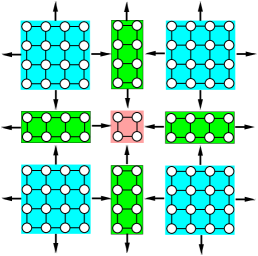
Figure 3: The local structure of another redundant region graph for the 2D model of figure 1. Each square region (cyan color) contains $4\times 4$ vertices and is parental to four rod regions, its counting number is $c=1$; each rod region (green color) contains $2\times 4$ vertices and is parental to two plaquette regions, its counting number is $c=-1$; each plaquette region (pink color) contains $2\times 2$ vertices, its counting number is $c=1$. For simplicity we do not show the small squares of figure 1 here but use a small edge between two vertices to indicate a coupling interaction.

To include more local correlations in the SGBP equations, we also consider another ideal redundant region graph (referred to as $R_{2D}^{n=4}$, see figure 3) for the 2D system (2). This region graph has the same topology as $R_{2D}^{n=2}$. The only difference is that each vertex region now becomes a plaquette region of $2\times 2$ vertices, and each square region now contains $4\times 4$ vertices. The SGBP equations for this region graph are similar to equations (5) and (34).

For the cubic lattice systems we consider a simple 3D extension of the region graph of figure 1. This extended region graph (later referred to as $R_{3D}^{n=2}$) has four types of regions: cube regions, surface regions, rod regions, and vertex regions. Each $2\times 2\times 2$ cubic cell of the 3D lattice forms a cube region of the region graph, it is parental to six surface regions, and its counting number is $c=1$; each $2\times 2$ plaquette of the lattice forms a surface region, it is parental to four rod regions and has counting number $c=-1$; each pair of nearest neighboring vertices of the lattice forms a rod region (it is parental to two vertex regions, and its counting number is $c=1$); and each vertex region contains only one single vertex, with counting number $c=-1$. The SGBP equations for such a 3D region graph are much more simplified in comparison with the original GBP equations.

We are mainly interested in the spontaneous emergence of collective behaviors, therefore we set the external field on each vertex to be zero ($h_{i}^{0}=0$ for all the vertices $i$).

5.1 The 2D Ising model

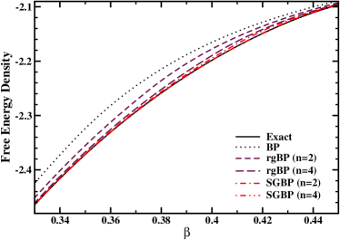
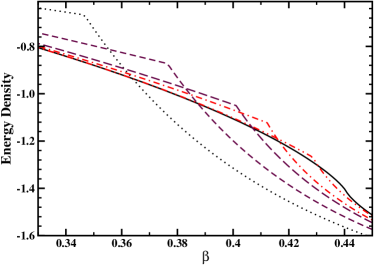
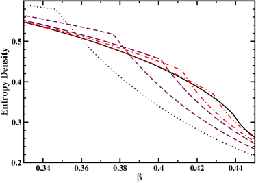
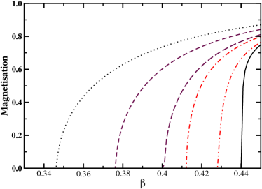
Figure 4: Results on the 2D ferromagnetic Ising model obtained by the SGBP equations, the rgBP equations of [7], and the conventional BP equation: (a) free energy density; (b) mean energy density; (c) entropy density; (d) magnetisation (mean spin value of a single vertex). The solid lines denote the exact results of [22]. The parameter $n$ of the SGBP equations and the rgBP equations is the number of vertices on each side of the maximal square region of the region graph. For the SGBP curves, $n=2$ and $n=4$ correspond to the region graph of figure 1 and figure 3, respectively. The region graphs at $n=2$ and $n=4$ for the rgBP equations are described in [7].

First we consider the simplest case, namely the ferromagnetic Ising model on an infinite square lattice with periodic boundary conditions. As the system has no disorder the SGBP equations can be easily solved at all temperatures. In figure 4 we compare the results obtained by the SGBP equations with the exact results of Onsager [22] and with the results obtained through the region graph belief propagation (rgBP) equations (see [7, 18] for details).

For the SGBP equations on a given region graph, we perform linear stability analysis to determine precisely the instability point of the paramagnetic solution, similar to that performed in [7]. The predicted transition inverse temperatures by the SGBP equations using the region graph $R_{2D}^{n=2}$ and $R_{2D}^{n=4}$ are, respectively, $\beta_{c}\approx 0.4126$ and $\beta_{c}\approx 0.429$. These values are rather close to the exactly known critical inverse temperature value of $\beta_{c}^{(exact)}\approx 0.4407$ [23], they are much improved over the predicted value of $\beta_{c}\approx 0.3466$ by the conventional BP method and the predicted values of $\beta_{c}\approx 0.3765$ and $\beta_{c}\approx 0.401$ by the rgBP equations on two non-redundant region graphs [7].

The SGBP equations also give better predictions on the free energy density, the mean energy density, the entropy density, and the mean magnetisation of the system, see figure 4. Using the region graph $R_{2D}^{n=4}$, the predicted values of the SGBP equations on the free energy density, energy density, and entropy density become very close to the exactly known results. The prediction power of the SGBP equations will be further improved if we consider more local correlations by enlarging each region of figure 3 while keeping unchanged the topology of this region graph.

5.2 The 2D Edwards-Anderson model

Because of the existence of multiple directed paths between some pairs of regions in the redundant region graph $R_{2D}^{n=2}$ or $R_{2D}^{n=4}$, the SGBP equations on some of the directed edges are redundant and can be dropped from the numerical iteration process (see discussion in the last paragraph of section 4). If instead the SGBP equations on all the directed edges of the region graph are used in the iteration process, the paramagnetic solution of the SGBP equations will be unstable even at $\beta=0$ ($T=\infty$).

In our numerical implementations for the 2D Edwards-Anderson model we still keep the SGBP equations on all the directed edges but add a damping effect to the SGBP equations to facilitate the convergence. We notice that the paramagnetic solution of the SGBP equations on the region graphs $R_{2D}^{n=2}$ and $R_{2D}^{n=4}$ fail to be stable at low temperatures even for optimally adjusted magnitude of the damping effect. However, the $\pm J$ EA model on 2D square lattice is believed to have no finite-temperature spin glass phase [24]. Therefore only the paramagnetic solution of the SGBP equations are qualitatively correct, even if it is unstable at low temperatures.

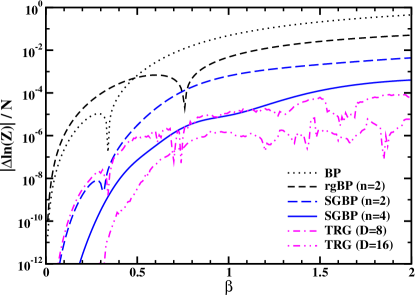
Figure 5: Difference $\Delta\ln Z$ between the exactly calculated value of $\ln Z$ and the value of $\ln Z$ obtained by BP, rgBP with $n=2$, SGBP with $n=2$ and $n=4$, and tensor renormalisation group (TRG) with cutoff parameter $D=8$ and $D=16$. All the numerical calculations are performed on a single instance of the 2D EA model with side length $L=64$ and periodic boundary conditions (the total number of vertices is $N=64^{2}$).

Since the free energy of a given instance of the EA model on a periodic square lattice with side length $L$ can be computed exactly in polynomial time [25], we can compare the free energy $\tilde{F}_{0}$ of the paramagnetic solution of the SGBP equations with the exact value, see figure 5. The SGBP results on the region graph $R_{2D}^{n=4}$ are comparable to the results obtained by the tensor renormalisation group (TRG) method [26] with cutoff parameter $D=8$ but are worse than the TRG results with cutoff parameter $D=16$. We expect that the performance of the SGBP equations will be further improved by enlarging the side length $n$ of the square regions. An advantage of the SGBP message passing approach is that it can simultaneously give the marginal probability distributions $\tilde{\omega}_{\mu}(\underline{x}_{\mu})$ for all the regions $\mu$.

5.3 The 3D Ising model and Edwards-Anderson model

The structure of a simple redundant region graph $R_{3D}^{n=2}$ for the 3D Ising model and EA model is described at the beginning of section 5. This region graph is formed by cube regions, surface regions, rod regions and vertex regions. Each cube region contains $n\times n\times n$ vertices with $n=2$. Linear stability analysis of the SGBP equations predicts that the ferromagnetic transition occurs at the critical inverse temperature $\beta_{c}\approx 0.2183$, which is very close to the value of $\beta_{c}\approx 0.2217$ obtained by Monte Carlo simulations [27] and the higher-order tensor renormalisation group (TRG) method [28]. As a comparison, the critical inverse temperature predicted by the BP approximation is $\beta_{c}\approx 0.2027$.

The magnetisation values predicted by the BP and SGBP equations are compared with the Monte Carlo simulation results of [27] in figure 7. It is evident that the performance of SGBP improves considerably over that of BP.

We also perform linear stability analysis on the paramagnetic solution of the SGBP equations for the 3D EA model (2). The stability threshold $\beta_{c}$ of the SGBP paramagnetic solution on the region graph $R_{3D}^{n=2}$ depends on the particular disorder instance. For each cubic lattice of side length $L$ under the periodic boundary condition, we generate $32$ independent realisations of the coupling constants $\{J_{ij}\}$ and then obtain the value of $\beta_{c}$ for each disorder realisation. The relationship between the mean value of $\beta_{c}$ and lattice size $L$ is shown in figure 7. The mean $\beta_{c}$ value decreases with lattice side length $L$ and appears to approach the value of $\beta_{c}\approx 0.505$ at $L\rightarrow\infty$. As a comparison, Monte Carlo simulations predicted that the spin glass phase transition occurs at $\beta_{c}\approx 0.893$ (see [29] and references therein). We believe that if we enlarge the side length $n$ of the maximal cube region of the used region graph, the critical value $\beta_{c}$ at $L=\infty$ will increase and be much more closer to the value predicted by Monte Carlo simulations.

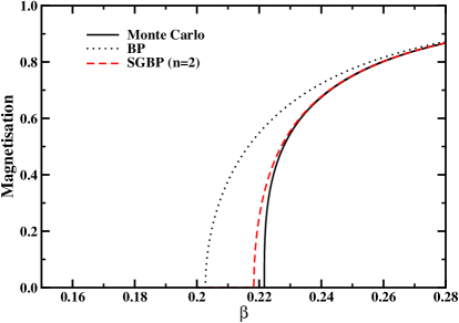
Figure 6: Mean magnetisation of the 3D Ising model as obtained by the SGBP equations (using region graph $R_{3D}^{n=2}$), the BP equations, and Monte Carlo simulations [27].

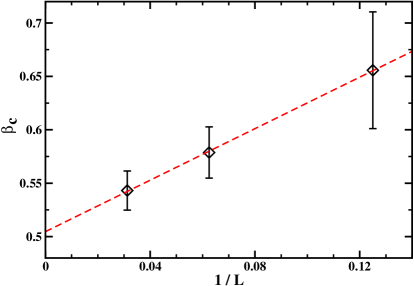
Figure 7: The inverse temperature $\beta_{c}$ for the instability of the paramagnetic solution of the SGBP equations on the 3D EA model with lattice side length $L$. The dashed line is the fitting curve of $\beta_{c}=0.505+1.20/L$.

6 Conclusion

In summary, we presented an alternative way of deriving a set of generalized belief propagation (GBP) equations for a general lattice statistical physical system. Based on this derivation we proposed a way of simplifying the GBP equations. We also pointed out that, due to the existence of redundance in the region graph, some of the simplified generalized belief propagation (SGBP) equations can be ignored in the numerical iteration process. We applied the set of SGBP equations to the two-dimensional and three-dimensional Ising model and Edwards-Anderson model. The numerical results confirmed that the SGBP message-passing approach significantly outperforms the conventional BP approach in treating short-range correlations. Hopefully this work will stimulate further developments of the SGBP message-passing approach and the applications of this approach to finite-dimensional disordered systems and finite-dimensional optimisation problems.

The three-dimensional Edwards-Anderson model (2) is in the spin glass phase at low temperatures, with broken ergodicity. To describe the low-temperature spin glass property of the EA model, the effects of ergodicity-breaking need to explicitly considered in the SGBP equations. This issue remains to be solved.

This work was supported by the Knowledge Innovation Program of Chinese Academy of Sciences (No. KJCX2-EW-J02), and the National Science Foundation of China (grant No. 11121403 and 11225526).

References

References

- [1] Kikuchi R 1951 Phys. Rev. 81 988–1003
- [2] An G 1988 J. Stat. Phys. 52 727–734
- [3] Morita T, Suzuki M, Wada K and Kaburagi M (eds) 1994 Foundations and Applications of Cluster Variation Method and Path Probability Method (Prog. Theor. Phys. Suppl. vol 115) (Physical Society of Japan)
- [4] Opper M and Saad D (eds) 2001 Advanced Mean Field Methods: Theory and Practice (Cambridge, MA: MIT Press)
- [5] Pelizzola A 2005 J. Phys. A: Meth. Gen. 38 R309–R339
- [6] Rizzo T, Lage-Castellanos A, Mulet R and Ricci-Tersenghi F 2010 J. Stat. Phys. 139 375–416
- [7] Zhou H J and Wang C 2012 J. Stat. Phys. 148 513–547
- [8] Bethe H A 1935 Proc. R. Soc. London A 150 552–575
- [9] Peierls R 1936 Proc. Camb. Phil. Soc. 32 477–481
- [10] Peierls R 1936 Proc. R. Soc. London A 154 207–222
- [11] Chang T S 1937 Proc. R. Soc. London A 161 546–563
- [12] Mézard M, Parisi G and Virasoro M A 1987 Spin Glass Theory and Beyond (Singapore: World Scientific)
- [13] Mézard M and Montanari A 2009 Information, Physics, and Computation (New York: Oxford Univ. Press)
- [14] Pearl J 1988 Probabilistic Reasoning in Intelligent Systems: Networks of Plausible Inference (San Franciso, CA, USA: Morgan Kaufmann)
- [15] Yedidia J S, Freeman W T and Weiss Y 2005 IEEE Trans. Inf. Theory 51 2282–2312
- [16] Edwards S F and Anderson P W 1975 J. Phys. F: Met. Phys. 5 965–974
- [17] Frey B J 1998 Graphical Models for Machine Learning and Digital Communication (Cambridge, MA: MIT Press)
- [18] Zhou H J, Wang C, Xiao J Q and Bi Z 2011 J. Stat. Mech.: Theo. Exp. L12001
- [19] Lage-Castellanos A, Mulet R, Ricci-Tersenghi F and Rizzo T 2011 Phys. Rev. E 84 046706
- [20] Domínguez E, Lage-Catellanos A, Mulet R, Ricci-Tersenghi F and Rizzo T 2011 J. Stat. Mech.: Theor. Exp. P12007
- [21] Lage-Castellanos A, Mulet R, Ricci-Tersenghi F and Rizzo T 2013 J. Phys. A: Math. Theor. 46 135001
- [22] Onsager L 1944 Phys. Rev. 65 117–149
- [23] Kramers H A and Wannier G H 1941 Phys. Rev. 60 252–262
- [24] Thomas C K, Huse D A and Middleton A A 2011 Phys. Rev. Lett. 107 047203
- [25] Barahona F 1982 J. Phys. A: Math. Gen. 15 3241–3253
- [26] Levin M and Nave C P 2007 Phys. Rev. Lett. 99 120601
- [27] Talapov A L and Blöte H W J 1996 J. Phys. A: Math. Gen. 29 5727–5733
- [28] Xie Z Y, Chen J, Qin M P, Zhu J W, Yang L P and Xiang T 2012 Phys. Rev. B 86 045139
- [29] Katzgraber H G, Körner M and Young A P 2006 Phys. Rev. B 73 224432