Spontaneous ferromagnetism in the spinor Bose gas with Rashba spin-orbit coupling

Abstract

We show that in the two-component Bose gas with Rashba spin-orbit coupling an arbitrarily small attractive interaction between bosons with opposite spin induces spontaneous ferromagnetism below a finite critical temperature $T_{c}$. In the ferromagnetic phase the single-particle spectrum exhibits a unique minimum in momentum space in the direction of the magnetization. For sufficiently small temperatures below $T_{c}$ the bosons eventually condense into the unique state at the bottom of the spectrum, forming a ferromagnetic Bose-Einstein condensate.

I Introduction

Due to recent progress in the field of ultracold gases, spinor Bose-Einstein condensates with various types of spin-orbit coupling can now be realized experimentally Lin09a ; Dalibard11 by using spatially varying laser fields to couple internal pseudo-spin degrees of freedom to the momentum. These experiments have motivated many theoretical investigations of spin-orbit coupled multi-component Bose gases Stanescu08 ; Wang10 ; Gopalakrishnan11 ; Ho11 ; Ozawa11 ; Barnett12 ; Sedrakyan12 ; Hu12 ; Cui12 ; Liao12 ; Li12 ; Zhou13 ; Yu13 . Of particular interest have been two-component bosons with isotropic Rashba-type Rashba60 spin-orbit coupling, where in the absence of interactions the energy dispersion assumes a minimum on a circle in momentum space Stanescu08 . If the bosons do not condense, such a surface in momentum space can be called a Bose surface, in analogy with the Fermi surface of an electronic system Paramekanti02 ; Sachdev02 . Of course, bosons do not obey the Pauli exclusion principle, so that the Bose surface cannot be the boundary between occupied and unoccupied states; however, the Bose surface defines the location of the low-energy excitations in the system, similar to the Fermi surface of an electronic system.

The fact that Bose-Einstein condensation (BEC) in Bose systems where the dispersion has degenerate minima on a surface in momentum space differs qualitatively from conventional BEC has been pointed out a long time ago by Yukalov Yukalov78 . He studied BEC in an interacting Bose system whose energy dispersion is minimal on a sphere in momentum space. Assuming that the bosons condense with equal weight into all states on this sphere, he showed that the condensed state does not exhibit off-diagonal long-range order and is also not superfluid.

Due to the degeneracy of the single-particle energy in the spinor Bose gas with Rashba-type spin-orbit coupling, in the non-interacting limit BEC is prohibited at any finite temperature. Hence, finite temperature BEC in this system must be an interaction effect Ozawa11 ; Hu12 . Interactions are expected to remove the ground state degeneracy and various types of exotic ground states have been proposed Stanescu08 ; Wang10 ; Gopalakrishnan11 ; Ho11 ; Ozawa11 ; Barnett12 ; Sedrakyan12 ; Hu12 ; Cui12 ; Liao12 ; Li12 ; Zhou13 ; Yu13 . Which phase is realized experimentally depends on the specific properties of the interaction. At this point a generally accepted agreement on the nature of the ground state in the spinor Bose gas with Rashba-type spin-orbit coupling has not been reached.

Phase transitions in systems whose fluctuation spectrum exhibits minima on a surface in momentum space form their own universality class, the so-called Brazovskii universality class Brazovskii75 ; for example, the critical behavior in cholesteric liquid crystals belongs to this class Hohenberg95 . Because scaling transformations and mode elimination in renormalization group calculations should be defined relative to the low-energy manifold, the classification of interaction vertices in systems belonging to the Brazovskii universality class is different from the corresponding classification in systems where the low-energy manifold consists of a single point; in particular, all two-body scattering processes where the momenta of the incoming and the outgoing particles lie on the low-energy manifold are marginal, so that in renormalization group calculations one should keep track of infinitely many marginal couplings. Note that also normal fermions belong to the Brazovskii universality class, because the Fermi surface can be identified with the low-energy manifold relative to which scaling transformations should be defined Shiwa06 ; Kopietz01 ; Kopietz10 . Two-component bosons with Rashba-type spin-orbit coupling are therefore another example for a quantum system which belongs to the Brazovskii universality class.

In this work we shall further investigate interaction effects on spinor Bose gases with Rashba-type spin-orbit coupling. We shall consider the specific case where the interaction $g_{\bot}$ between two bosons with opposite pseudo-spin is attractive. We find that in this case for any finite density an arbitrarily small interaction $g_{\bot}<0$ leads to spontaneous ferromagnetism below some finite temperature $T_{c}$. In the ferromagnetic phase, the single-particle dispersion has a unique minimum in momentum space, so that the bosons eventually condense at some temperature $T_{\rm BEC}<T_{c}$ into the unique single-particle state at the bottom of the spectrum.

II Spin-orbit coupled bosons

We consider a two-component Bose gas with Rashba spin-orbit coupling and a two-body interaction which is invariant under rotations around the $z$-axis in spin-space. The Hamiltonian is given by ${\cal{H}}={\cal{H}}_{0}+{\cal{H}}_{\rm int}$, with

$${\cal{H}}_{0} = \sum_{\bm{k}}(a^{\dagger}_{\bm{k}\uparrow},a^{\dagger}_{\bm{k}\downarrow})\left[\frac{\bm{k}^{2}-2k_{0}{\bm{k}}_{\bot}\cdot\bm{\sigma}}{2m}\right]\left(\begin{array}[]{c}a_{\bm{k}\uparrow}\\ a_{\bm{k}\downarrow}\end{array}\right),$$ (3)

$${\cal{H}}_{\rm int} = \frac{1}{2V}\sum_{\bm{k}_{1}^{\prime}\bm{k}_{2}^{\prime}\bm{k}_{2}\bm{k}_{1}}\sum_{\sigma_{1}\sigma_{2}}\delta_{\bm{k}_{1}^{\prime}+\bm{k}_{2}^{\prime},\bm{k}_{2}+\bm{k}_{1}}$$ (4)

$$\times U_{\sigma_{1}\sigma_{2}}(\bm{k}_{1}^{\prime},\bm{k}_{2}^{\prime};\bm{k}_{2},\bm{k}_{1})a^{\dagger}_{\bm{k}_{1}^{\prime}\sigma_{1}}a^{\dagger}_{\bm{k}_{2}^{\prime}\sigma_{2}}a_{\bm{k}_{2}\sigma_{2}}a_{\bm{k}_{1}\sigma_{1}},\hskip 19.91692pt$$

where $\bm{k}_{\bot}=k_{x}\hat{\bm{x}}+k_{y}\hat{\bm{y}}$ is the projection of the wave-vector $\bm{k}$ onto the $xy$-plane, and the components of the vector operator $\bm{\sigma}$ are the usual Pauli matrices. The wave-vector $k_{0}$ measures the strength of the spin-orbit coupling. The invariance of the interaction under spin-rotations around the $z$-axis implies that the function $U_{\sigma_{1}\sigma_{2}}(\bm{k}_{1}^{\prime},\bm{k}_{2}^{\prime};\bm{k}_{2},\bm{k}_{1})$ is symmetric with respect to the simultaneous permutation of its incoming and outgoing labelsKopietz10

$$U_{\sigma_{1}\sigma_{2}}(\bm{k}_{1}^{\prime},\bm{k}_{2}^{\prime};\bm{k}_{2},\bm{k}_{1})=U_{\sigma_{2}\sigma_{1}}(\bm{k}_{2}^{\prime},\bm{k}_{1}^{\prime};\bm{k}_{1},\bm{k}_{2}).$$ (5)

For simplicity, we assume that the bare interaction is momentum independent, so that the interaction is characterized by three different coupling constants

$$g_{\uparrow}=U_{\uparrow\uparrow}(0);\;\;g_{\downarrow}=U_{\downarrow\downarrow}(0);\;\;g_{\bot}=U_{\uparrow\downarrow}(0)=U_{\downarrow\uparrow}(0),$$ (6)

and ${\cal{H}}_{\rm int}$ simplifies to

$${\cal{H}}_{\rm int} = \frac{1}{2V}\sum_{\bm{k}_{1}^{\prime}\bm{k}_{2}^{\prime}\bm{k}_{2}\bm{k}_{1}}\delta_{\bm{k}_{1}^{\prime}+\bm{k}_{2}^{\prime},\bm{k}_{2}+\bm{k}_{1}}\Bigl{[}g_{\uparrow}a^{\dagger}_{\bm{k}_{1}^{\prime}\uparrow}a^{\dagger}_{\bm{k}_{2}^{\prime}\uparrow}a_{\bm{k}_{2}\uparrow}a_{\bm{k}_{1}\uparrow}$$ (7)

$$+g_{\downarrow}a^{\dagger}_{\bm{k}_{1}^{\prime}\downarrow}a^{\dagger}_{\bm{k}_{2}^{\prime}\downarrow}a_{\bm{k}_{2}\downarrow}a_{\bm{k}_{1}\downarrow}+2g_{\bot}a^{\dagger}_{\bm{k}_{1}^{\prime}\uparrow}a^{\dagger}_{\bm{k}_{2}^{\prime}\downarrow}a_{\bm{k}_{2}\downarrow}a_{\bm{k}_{1}\uparrow}\Bigr{]}.$$

Introducing the usual field operators

$$\hat{\psi}_{\sigma}(\bm{r})=\frac{1}{\sqrt{V}}\sum_{\bm{k}}e^{i\bm{k}\cdot\bm{r}}a_{\bm{k}\sigma},$$ (8)

and the corresponding density operators $\hat{\rho}_{\sigma}(\bm{r})=\hat{\psi}^{\dagger}_{\sigma}(\bm{r})\hat{\psi}_{\sigma}(\bm{r})$ the interaction can be written as follows,

$${\cal{H}}_{\rm int} = \frac{1}{2}\int d^{D}r\Bigl{[}g_{\uparrow}:\hat{\rho}^{2}_{\uparrow}(\bm{r}):+g_{\downarrow}:\hat{\rho}^{2}_{\downarrow}(\bm{r}):$$ (9)

$$\hskip 36.98857pt+2g_{\bot}:\hat{\rho}_{\uparrow}(\bm{r})\hat{\rho}_{\downarrow}(\bm{r}):\Bigr{]}\;,$$

where $:\ldots:$ denotes normal ordering. Assuming for simplicity $g_{\uparrow}=g_{\downarrow}=g_{\parallel}$, we may write the interaction as

$${\cal{H}}_{\rm int}=\frac{1}{2}\int d^{D}r\Bigl{[}g_{\rho}:\hat{\rho}^{2}(\bm{r}):+g_{\sigma}:\hat{\sigma}^{2}(\bm{r}):\Bigr{]},$$ (10)

where $\hat{\rho}=\hat{\rho}_{\uparrow}+\hat{\rho}_{\downarrow}$ and $\hat{\sigma}=\hat{\rho}_{\uparrow}-\hat{\rho}_{\downarrow}$ represent the density and the spin density, and the associated couplings are

$$g_{\rho}=\frac{1}{2}(g_{\parallel}+g_{\bot}),\;\;\;g_{\sigma}=\frac{1}{2}(g_{\parallel}-g_{\bot}).$$ (11)

From Eq. (10) it is clear that for $g_{\sigma}<0$ (i.e., $g_{\bot}>g_{\parallel}$) states with a finite spin-density are favored; an example is the standing wave spin-striped state proposed in Ref. [Wang10, ], where the bosons condense simultaneously into two momentum states with opposite momenta on the low-energy manifold in momentum space. On the other hand, $g_{\sigma}>0$ favors states with vanishing spin density, such as plane wave condensate where the bosons condense into a single momentum state, or the charge striped states discussed in Refs. [Ho11, ; Li12, ]. In this work, we focus on the case where $g_{\bot}$ is negative. We show below that even for infinitesimally small $g_{\bot}<0$ the system exhibits spontaneous ferromagnetism in the plane of the spin-orbit coupling at sufficiently low temperatures.

To set up our notation, let us review the diagonalization of ${\cal{H}}_{0}$. Performing a momentum-dependent rotation in spin space around an axis $\bm{\theta}_{\bm{k}}/|\bm{\theta}_{\bm{k}}|$ with angle $|\bm{\theta}_{\bm{k}}|$,

$$\left(\begin{array}[]{c}a_{\bm{k}\uparrow}\\ a_{\bm{k}\downarrow}\end{array}\right)=e^{-\frac{i}{2}{\bm{\sigma}}\cdot\bm{\theta}_{\bm{k}}}\left(\begin{array}[]{c}a_{\bm{k}-}\\ a_{\bm{k}+}\end{array}\right),$$ (12)

and using the fact thatRueckriegel12

$$e^{\frac{i}{2}{\bm{\sigma}}\cdot\bm{\theta}_{\bm{k}}}\bm{\sigma}e^{-\frac{i}{2}{\bm{\sigma}}\cdot\bm{\theta}_{\bm{k}}}=e^{\bm{\theta}_{\bm{k}}\times}\bm{\sigma},$$ (13)

we obtain

$${\cal{H}}_{0}=\sum_{\bm{k}}(a^{\dagger}_{\bm{k}-},a^{\dagger}_{\bm{k}+})\left[\frac{\bm{k}^{2}-2k_{0}{\bm{k}}_{\bot}\cdot(e^{\bm{\theta}_{\bm{k}}\times}\bm{\sigma})}{2m}\right]\left(\begin{array}[]{c}a_{\bm{k}-}\\ a_{\bm{k}+}\end{array}\right).$$ (14)

We now choose the rotation matrix $e^{\bm{\theta}_{\bm{k}}\times}$ such that it rotates the z-axis into the direction $\hat{\bm{k}}_{\bot}=\bm{k}_{\bot}/|\bm{k}_{\bot}|$, i.e.,

$$\hat{\bm{k}}_{\bot}=e^{\bm{\theta}_{\bm{k}}\times}\hat{\bm{z}},$$ (15)

which can be achieved by setting

$$\bm{\theta}_{\bm{k}}=\frac{\pi}{2}\hat{\bm{z}}\times\hat{\bm{k}}_{\bot}.$$ (16)

Due to the rotational invariance of the scalar product, we may hence write

$$\hat{{\bm{k}}}_{\bot}\cdot(e^{\bm{\theta}_{\bm{k}}\times}\bm{\sigma})=(e^{\bm{\theta}_{\bm{k}}\times}\hat{\bm{z}})\cdot(e^{\bm{\theta}_{\bm{k}}\times}\bm{\sigma})=\hat{\bm{z}}\cdot\bm{\sigma}=\sigma^{z}.$$ (17)

Our rotation matrix in spin space is then explicitly given by

$$e^{-\frac{i}{2}{\bm{\sigma}}\cdot\bm{\theta}_{\bm{k}}} = \cos\left(\frac{\theta_{\bm{k}}}{2}\right)\left(\begin{array}[]{cc}1&0\\ 0&1\end{array}\right)-i\sin\left(\frac{\theta_{\bm{k}}}{2}\right)\bm{\sigma}\cdot\hat{\bm{\theta}}_{\bm{k}}$$ (20)

$$= \frac{1}{\sqrt{2}}\left[\left(\begin{array}[]{cc}1&0\\ 0&1\end{array}\right)-i\bm{\sigma}\cdot(\hat{\bm{z}}\times\hat{\bm{k}}_{\bot})\right]$$ (23)

$$= \frac{1}{\sqrt{2}}\left(\begin{array}[]{cc}1&-\hat{k}_{x}+i\hat{k}_{y}\\ \hat{k}_{x}+i\hat{k}_{y}&1\end{array}\right)$$ (26)

$$= \frac{1}{\sqrt{2}}\left(\begin{array}[]{cc}1&-e^{-i\varphi_{\bm{k}}}\\ e^{i\varphi_{\bm{k}}}&1\end{array}\right),$$ (29)

where in the last line we have set $\hat{k}_{x}=\cos\varphi_{\bm{k}}$ and $\hat{k}_{y}=\sin\varphi_{\bm{k}}$. In the new basis (which we shall call the helicity basis) the non-interacting part of the Hamiltonian is

$${\cal{H}}_{0}=\sum_{\bm{k}}\sum_{\lambda=\pm}E_{\bm{k}\lambda}a^{\dagger}_{\bm{k}\lambda}a_{\bm{k}\lambda},$$ (30)

with energy dispersions

$$E_{\bm{k}\lambda}=\frac{\bm{k}^{2}}{2m}+\lambda v_{0}|\bm{k}_{\bot}|=\frac{(|\bm{k}_{\bot}|+\lambda k_{0})^{2}+k_{z}^{2}-k_{0}^{2}}{2m}.$$ (31)

Here $v_{0}=k_{0}/m$ and the helicity index $\lambda=\pm$ labels the two branches of the dispersion. A graph of these dispersions is shown in Fig. 1.

Figure 1: (Color online) Graph of the energy dispersions (31) of the spinor Bose gas with Rashba-type spin-orbit coupling. The minimum of the lower helicity branch is a circle in the plane $k_{z}=0$ with radius $k_{0}$. The spacing between contours scales quartically.

Note that the energy $E_{\bm{k},-}$ assumes its minimum $-k_{0}^{2}/(2m)$ on a circle of radius $k_{0}$ in the $xy$-plane, while $E_{\bm{k},+}$ is non-negative and vanishes only at $\bm{k}=0$. Due to the momentum-dependent rotation in spin-space, the interaction vertices in the helicity basis acquire a momentum-dependence. For completeness we give the properly symmetrized expressions for these vertices in Appendix A. For our mean-field calculation it is more convenient to work in the original spin basis.

III Mean-field theory for transverse ferromagetism

III.1 Derivation of the mean-field equations

To study transverse ferromagnetism we add a uniform magnetic field $\bm{h}_{\bot}$ in the $xy$-plane, so that the non-interacting part of our Hamiltonian is now given by

$${\cal{H}}_{0} = \sum_{\bm{k}}(a^{\dagger}_{\bm{k}\uparrow},a^{\dagger}_{\bm{k}\downarrow})\left[\frac{\bm{k}^{2}-2k_{0}{\bm{k}}_{\bot}\cdot\bm{\sigma}}{2m}-\bm{h}_{\bot}\cdot\bm{\sigma}\right]\left(\begin{array}[]{c}a_{\bm{k}\uparrow}\\ a_{\bm{k}\downarrow}\end{array}\right).$$ (34)

For convenience we measure the magnetic field in units of energy. The system exhibits spontaneous ferromagnetism if the magnetization remains finite when $\bm{h}_{\bot}\rightarrow 0$. The spin-rotational invariance with respect to rotations around the $z$-axis is then spontaneously broken. While in the symmetric phase the self-energies $\Sigma_{\sigma\sigma\prime}$ are diagonal in the spin-labels, in the symmetry broken phase there are finite off-diagonal components $\Sigma_{\uparrow\downarrow}$ and $\Sigma_{\downarrow\uparrow}$. Within the self-consistent Hartree-Fock approximation the self-energies are independent of momentum and frequency if we start from a momentum-independent bare interaction. The mean-field Hamiltonian is therefore of the form

$${\cal{H}}_{\rm MF}={\cal{H}}_{0}+\sum_{\bm{k}}(a^{\dagger}_{\bm{k}\uparrow},a^{\dagger}_{\bm{k}\downarrow})\left(\begin{array}[]{cc}\Sigma_{\uparrow\uparrow}&\Sigma_{\uparrow\downarrow}\\ \Sigma_{\downarrow\uparrow}&\Sigma_{\downarrow\downarrow}\end{array}\right)\left(\begin{array}[]{c}a_{\bm{k}\uparrow}\\ a_{\bm{k}\downarrow}\end{array}\right).$$ (36)

Within the self-consistent Hartree-Fock approximation the self-energies are

$$\Sigma_{\uparrow\uparrow} = 2g_{\uparrow}\rho_{\uparrow}+g_{\bot}\rho_{\downarrow},$$ (37a)

$$\Sigma_{\downarrow\downarrow} = 2g_{\downarrow}\rho_{\downarrow}+g_{\bot}\rho_{\uparrow},$$ (37b)

$$\Sigma_{\uparrow\downarrow} = g_{\bot}\rho_{\downarrow\uparrow},$$ (37c)

$$\Sigma_{\downarrow\uparrow} = g_{\bot}{\rho}_{\uparrow\downarrow},$$ (37d)

where we have introduced the densities

$$\rho_{\sigma} = \frac{1}{V}\sum_{\bm{k}}\langle a^{\dagger}_{\bm{k}\sigma}a_{\bm{k}\sigma}\rangle,$$ (38)

$$\rho_{\uparrow\downarrow} = \rho_{\downarrow\uparrow}^{\ast}=\frac{1}{V}\sum_{\bm{k}}\langle a^{\dagger}_{\bm{k}\uparrow}a_{\bm{k}\downarrow}\rangle.$$ (39)

Here the expectation values should be evaluated with the grand canonical density matrix associated with the mean-field Hamiltonian (36). Note that our mean-field decoupling excludes states with broken translational invariance. This will be justified a posteriori from the fact that the irreducible ferromagnetic susceptibility is exponentially large at low temperatures [see Eq. (LABEL:eq:chilow)], such that, at least at weak coupling, the ferromagnetic instability is dominant. Keeping in mind that $\rho_{\uparrow\downarrow}=M_{x}+iM_{y}$ can be expressed in terms of the components of the transverse magnetization $\bm{M}_{\bot}=M_{x}\hat{\bm{x}}+M_{y}\hat{\bm{y}}$, we see that the Cartesian components of the off-diagonal self-energies are proportional to the corresponding components of the magnetization,

$$\Sigma_{x} = \frac{1}{2}(\Sigma_{\uparrow\downarrow}+\Sigma_{\downarrow\uparrow})=g_{\bot}M_{x},$$ (40)

$$\Sigma_{y} = \frac{i}{2}(\Sigma_{\uparrow\downarrow}-\Sigma_{\downarrow\uparrow})=g_{\bot}M_{y}.$$ (41)

It is convenient to define in addition the self-energies

$$\Sigma_{z} = \frac{1}{2}(\Sigma_{\uparrow\uparrow}-\Sigma_{\downarrow\downarrow})=g_{\uparrow}\rho_{\uparrow}-g_{\downarrow}\rho_{\downarrow}-\frac{g_{\bot}}{2}(\rho_{\uparrow}-\rho_{\downarrow}),$$ (42)

$$\Sigma_{0} = \frac{1}{2}(\Sigma_{\uparrow\uparrow}+\Sigma_{\downarrow\downarrow})=g_{\uparrow}\rho_{\uparrow}+g_{\downarrow}\rho_{\downarrow}+\frac{g_{\bot}}{2}(\rho_{\uparrow}+\rho_{\downarrow}),\hskip 19.91692pt$$ (43)

and the wave-vector

$$\bm{p}=(\bm{h}_{\bot}-\bm{\Sigma})/v_{0},$$ (44)

where $\bm{\Sigma}=\Sigma_{x}\hat{\bm{x}}+\Sigma_{y}\hat{\bm{y}}+\Sigma_{z}\hat{\bm{z}}$ is proportional to the internal magnetic field induced by the interaction. The Hamiltonian can now be diagonalized via a momentum-dependent rotation in spin space of the form (12). The rotation matrix can be written as

$$e^{-\frac{i}{2}{\bm{\sigma}}\cdot\bm{\theta}_{\bm{k}}}=\left(\begin{array}[]{cc}\cos(\theta_{\bm{k}}/2)&-\sin(\theta_{\bm{k}}/2)e^{-i\varphi_{\bm{k}}}\\ \sin(\theta_{\bm{k}}/2)e^{i\varphi_{\bm{k}}}&\cos(\theta_{\bm{k}}/2)\end{array}\right),$$ (45)

where the rotation angles in the presence of an effective magnetic field $\bm{h}_{\bot}-\bm{\Sigma}=v_{0}\bm{p}$ are now given by

$$\cos\theta_{\bm{k}} = \frac{p_{z}}{|\bm{k}_{\bot}+\bm{p}|},$$ (46a)

$$\sin\theta_{\bm{k}} = \sqrt{1-\frac{p_{z}^{2}}{|\bm{k}_{\bot}+\bm{p}|^{2}}},$$ (46b)

$$\cos\varphi_{\bm{k}} = \frac{k_{x}+p_{x}}{\sqrt{(k_{x}+p_{x})^{2}+(k_{y}+p_{y})^{2}}},$$ (46c)

$$\sin\varphi_{\bm{k}} = \frac{k_{y}+p_{y}}{\sqrt{(k_{x}+p_{x})^{2}+(k_{y}+p_{y})^{2}}}.$$ (46d)

The energy dispersions of the eigenmodes are

$$E_{\bm{k}\lambda}=\frac{\bm{k}^{2}}{2m}+\Sigma_{0}+\lambda v_{0}|\bm{k}_{\bot}+\bm{p}|,$$ (47)

where $\lambda=\pm$ labels again the helicity of the modes. These dispersions are shown graphically in Fig. 2.

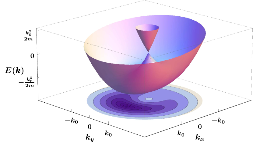
Figure 2: (Color online) Graph of the energy dispersions (47) of the spinor Bose gas with Rashba-type spin-orbit coupling and an effective magnetic field $\bm{h}_{\bot}-\bm{\Sigma}=v_{0}\bm{p}$ pointing in the direction of the positive $x$-axis. The lower helicity branch has a unique minimum at $\bm{k}_{0}=k_{0}\bm{p}/|\bm{p}|$. The spacing between contours scales quartically.

Obviously, for any finite $\bm{p}$ the degeneracy of the corresponding dispersion without magnetic field shown in Fig. 1 is completely removed, so that $E_{\bm{k},-}$ now has a unique minimum at $\bm{k}_{0}=k_{0}\bm{p}/|\bm{p}|$.

To derive a self-consistency equation for the transverse magnetization, we simply evaluate the off-diagonal density (39), using the grand canonical density matrix associated with the mean-field Hamiltonian on the right-hand side. We thus obtain

$$\rho_{\uparrow\downarrow} = M_{x}+iM_{y}=-\frac{1}{2V}\sum_{\bm{k}\lambda}\lambda\sin\theta_{\bm{k}}e^{i\varphi_{\bm{k}}}n_{\bm{k}\lambda},\hskip 19.91692pt$$ (48)

where

$$n_{\bm{k}\lambda}=\frac{1}{e^{\beta(E_{\bm{k}\lambda}-\mu)}-1}$$ (49)

is the average occupation of the mode with energy $E_{\bm{k}\lambda}$. Below we shall work at constant density, so that we should eliminate the chemical potential $\mu$ in favor of $\rho$. Therefore we need the diagonal densities (38),

$$\rho_{\sigma} = \frac{1}{2V}\sum_{\bm{k}}\sum_{\lambda}\left[1-\sigma\lambda\frac{p_{z}}{|\bm{k}_{\bot}+\bm{p}|}\right]n_{\bm{k}\lambda},$$ (50)

implying that the total density is

$$\rho=\sum_{\sigma}\rho_{\sigma}=\frac{1}{V}\sum_{\bm{k},\lambda}n_{\bm{k}\lambda}.$$ (51)

To show that the phase transition to the ferromagnetic state is continuous, it is useful to calculate the grand canonical potential, which in a mean-field approximation is given by

$${\Omega}(T,\mu,h)=T\sum_{\bm{k}}\sum_{\lambda=\pm}\ln\left[1-e^{-\beta(E_{\bm{k}\lambda}-\mu)}\right]-\langle{\cal{H}}_{\rm int}\rangle,$$ (52)

where the expectation value of the interaction part of the Hamiltonian is

$$\langle{\cal{H}}_{\rm int}\rangle/V = g_{\uparrow}\rho_{\uparrow}^{2}+g_{\downarrow}\rho_{\downarrow}^{2}+g_{\bot}(\rho_{\uparrow}\rho_{\downarrow}+\bm{M}_{\bot}^{2})$$ (53)

$$= \left(\frac{g_{\parallel}}{2}+\frac{g_{\bot}}{4}\right)\rho^{2}+g_{\bot}\bm{M}_{\bot}^{2},$$

and the second line holds for $g_{\uparrow}=g_{\downarrow}=g_{\parallel}$. For simplicity, let us now choose $\bm{h}_{\bot}=h\hat{\bm{x}}$ so that $\bm{M}_{\bot}=M\hat{\bm{x}}$. To explore the possibility of spontaneous transverse magnetization at constant density, we should consider the Gibbs potential

$$G(T,\rho,M) = \Omega(T,\mu,{h})+V(\mu\rho+{h}{{M}}),$$ (54)

where $\mu=\mu(\rho,M)$ and $h=h(\rho,M)$ should be determined by inverting the equations

$$\rho = -\frac{1}{V}\frac{\partial\Omega}{\partial\mu},\;\;\;M=-\frac{1}{V}\frac{\partial\Omega}{\partial h}.$$ (55)

To study spontaneous transverse ferromagnetism, we shall later take the limit $h\rightarrow 0$. For simplicity, we assume that $g_{\uparrow}=g_{\downarrow}=g_{\parallel}$, so that $\rho_{\uparrow}=\rho_{\downarrow}=\rho/2$ and $\Sigma_{0}=(g_{\parallel}+g_{\bot}/2)\rho$. As a consequence $\Sigma_{z}=0$ and $p_{z}=0$. Our self-consistency equation (48) then reduces to the following equation for the transverse magnetization,

$$\bm{M}_{\bot}=-\frac{1}{2V}\sum_{\bm{k}\lambda}\lambda\frac{{\bm{k}}_{\bot}+\bm{p}}{|\bm{k}_{\bot}+\bm{p}|}n_{\bm{k}\lambda}.$$ (56)

Note that $\bm{p}$ in the right-hand side depends again on $\bm{M}_{\bot}$ via Eqs. (44) and (40,41); for $g_{\uparrow}=g_{\downarrow}$ and $\bm{h}\rightarrow 0$ the relation between $\bm{p}$ and $\bm{M}_{\bot}$ is simply $\bm{p}=-g_{\bot}\bm{M}_{\bot}/v_{0}$. To determine the order of the phase transition for $h\rightarrow 0$, it is sufficient to consider the change in the free energy $F(T,\rho)=\Omega+V\mu\rho$ for arbitrary magnetization $M$,

$$\Delta F(T,\rho\;M)=F(T,\rho,h=0)_{M\neq 0}-F(T,\rho,h=0)_{M=0}.$$ (57)

The physical state of the system at vanishing external field is determined by $\partial\Delta F(T,\rho;M)/\partial M=0$, which is another way of deriving the self-consistency equation (56) for the order parameter $M$.

III.2 Spectral densities

To evaluate the integrals appearing in Eqs. (51) and (52), it is useful to introduce the density of states

$$\nu_{\lambda}(\epsilon,p)=\frac{1}{V}\sum_{\bm{k}}\delta(\epsilon-E_{\bm{k}\lambda})=\frac{1}{V}\sum_{\bm{k}^{\prime}}\delta(\epsilon-E_{\bm{k}^{\prime}-\bm{p},\lambda}),$$ (58)

where $p=(h-g_{\bot}M)/v_{0}$ and we have shifted $\bm{k}^{\prime}=\bm{k}+\bm{p}$ on the right-hand side. The density equation (51) can then be written as

$$\rho=\int_{-\infty}^{\infty}d\epsilon\sum_{\lambda}\nu_{\lambda}(\epsilon,p)\frac{1}{e^{\beta(\epsilon-\mu)}-1},$$ (59)

while our expression (52) for the grand canonical potential per volume becomes

$$\frac{\Omega(T,\mu,h)}{V} = T\int_{-\infty}^{\infty}d\epsilon\sum_{\lambda}\nu_{\lambda}(\epsilon,p)\ln[1-e^{-\beta(\epsilon-\mu)}]$$ (60)

$$- \frac{g_{\parallel}}{2}\rho^{2}-g_{\bot}\left(\frac{\rho^{2}}{4}+M^{2}\right).$$

It is also useful to rewrite the self-consistency equation for $\bm{M}_{\bot}=M\hat{\bm{x}}$ in terms of a generalized susceptibility as follows. Shifting $\bm{k}^{\prime}=\bm{k}+\bm{p}$ in Eq. (56) we obtain

$$M = -\frac{1}{2V}\sum_{\bm{k}^{\prime}\lambda}\lambda\frac{k_{x}^{\prime}}{|\bm{k}_{\bot}^{\prime}|}n_{\bm{k}^{\prime}-\bm{p},\lambda}.$$ (61)

We now introduce cylindrical coordinates in $\bm{k}^{\prime}$-space and perform a partial integration in the angular part. Rearranging terms we find that the self-consistency equation (61) can be written as

$$\frac{h}{M}=\frac{1}{\chi_{\bot}(M)}+g_{\bot},$$ (62)

where the irreducible susceptibility $\chi_{\bot}(M)$ is defined by

$$\chi_{\bot}(M)=-\frac{\beta}{2V}\sum_{\bm{k}^{\prime}\lambda}\frac{k^{\prime 2}_{y}}{|\bm{k}^{\prime}_{\bot}|k_{0}}\lambda n_{\bm{k}^{\prime}-\bm{p},\lambda}[n_{\bm{k}^{\prime}-\bm{p},\lambda}+1].$$ (63)

It is easy to see that $\chi_{\bot}(M)>0$, implying that, only for $g_{\bot}<0$, the magnetization $M$ can remain finite for $h\rightarrow 0$. From now on we shall therefore assume that $g_{\bot}$ is negative. In this case the magnetization in the broken symmetry phase satisfies the self-consistency equation

$$\chi_{\bot}(M)=-\frac{1}{g_{\bot}}.$$ (64)

Note that the physical susceptibility $M/h$ diverges at the critical point. To evaluate $\chi_{\bot}(M)$, we introduce the weighted density of states,

$${\sigma}_{\lambda}(\epsilon,p) = \frac{1}{V}\sum_{\bm{k}^{\prime}}\frac{k_{y}^{\prime 2}}{|\bm{k}_{\bot}^{\prime}|k_{0}}\delta(\epsilon-E_{\bm{k}^{\prime}-\bm{p},\lambda}).$$ (65)

Then we may write

$$\chi_{\bot}(M) = -\frac{\beta}{2}\int_{-\infty}^{\infty}d\epsilon\sum_{\lambda}\lambda\sigma_{\lambda}(\epsilon,p)\frac{e^{\beta(\epsilon-\mu)}}{[e^{\beta(\epsilon-\mu)}-1]^{2}}.\hskip 19.91692pt$$ (66)

Introducing cylindrical coordinates in $\bm{k}^{\prime}$-space in the above integrals defining $\nu_{\lambda}(\epsilon,p)$ and $\sigma_{\lambda}(\epsilon,p)$, the integrations over $k_{z}^{\prime}$ and $|\bm{k}_{\bot}^{\prime}|$ can be carried out exactly so that we can write these functions as one-dimensional angular integrals. The results can be written in the scaling form

$$\frac{\nu_{\lambda}(\epsilon,p)}{\nu_{0}} = \tilde{\nu}_{\lambda}\left(\frac{\epsilon-\Sigma_{0}-\frac{p^{2}}{2m}}{\epsilon_{0}},\frac{p}{k_{0}}\right),$$ (67)

$$\frac{\sigma_{\lambda}(\epsilon,p)}{\nu_{0}} = \tilde{\sigma}_{\lambda}\left(\frac{\epsilon-\Sigma_{0}-\frac{p^{2}}{2m}}{\epsilon_{0}},\frac{p}{k_{0}}\right),$$ (68)

where

$$\nu_{0}=\frac{mk_{0}}{2\pi},\qquad\epsilon_{0}=\frac{k_{0}^{2}}{2m}.$$ (69)

In Appendix B we give explicit expressions for the dimensionless scaling functions $\tilde{\nu}_{\lambda}(\tilde{\epsilon},\tilde{p})$ and $\tilde{\sigma}_{\lambda}(\tilde{\epsilon},\tilde{p})$ as one-dimensional integrals. In fact, for negative $\tilde{\epsilon}$ the remaining angular integration in the expressions for $\tilde{\nu}_{-}(\tilde{\epsilon},\tilde{p})$ and $\tilde{\sigma}_{-}(\tilde{\epsilon},\tilde{p})$ can also be done analytically, see Eqs. (B3) and (B5). Graphs of the scaling functions are shown in Fig. 3.

Figure 3: (Color online) (a) Graph of the scaling functions $\tilde{\nu}_{\pm}(\tilde{\epsilon},\tilde{p})$ of the density of states defined via Eq. (67) for $\tilde{p}=0.1$, see Eqs. (B1, B3). (b) Graph of the scaling functions $\tilde{\sigma}_{\pm}(\tilde{\epsilon},\tilde{p})$ of the weighted density of states defined via Eq. (68) for $\tilde{p}=0.1$, see Eqs. (B4, B5). The solid lines correspond to the scaling functions in the $\lambda=-1$ branch while the dashed lines are the scaling functions in the $\lambda=1$ branch. The insets show a closeup of the negative energy part of the spectral functions in the lower helicity branch. We use $\tilde{\epsilon}_{-}=\left(\epsilon_{-}-\Sigma_{0}-\left(p^{2}/2m\right)\right)/\epsilon_{0}$ and $\tilde{\epsilon}_{\ast}=\left(\epsilon_{\ast}-\Sigma_{0}-\left(p^{2}/2m\right)\right)/\epsilon_{0}$.

The behavior of the spectral densities $\nu_{-}(\epsilon,p)$ and $\sigma_{-}(\epsilon,p)$ associated with the negative energy branch is rather interesting. Both functions vanish if $\epsilon$ is smaller than the lower threshold energy

$$\epsilon_{-}=-\epsilon_{0}+\Sigma_{0}-v_{0}p.$$ (70)

Recall that in the absence of an external magnetic field $p=-\Sigma_{x}/v_{0}=(-g_{\bot})M/v_{0}$. For energies slightly above the lower threshold we obtain from Eqs. (B6, B7),

$$\frac{\nu_{-}(\epsilon,p)}{\nu_{0}} \sim \frac{\sqrt{2(1+\tilde{p})}}{\pi}\sqrt{\frac{\epsilon-\epsilon_{-}}{v_{0}p}},$$ (71)

$$\frac{\sigma_{-}(\epsilon,p)}{\nu_{0}} \sim \frac{\sqrt{1+\tilde{p}}}{3\pi}\left[\frac{\epsilon-\epsilon_{-}}{v_{0}p}\right]^{3/2},$$ (72)

where $\tilde{p}=p/k_{0}$. Eqs. (71, 72) can also be derived by expanding the energy dispersion $E_{\bm{k},-}$ of the lower branch around the minimum $\bm{k}_{0}=k_{0}\hat{\bm{x}}$ to quadratic order,

$$E_{\bm{k}_{0}+\bm{q},-}\approx\epsilon_{-}+\frac{q_{x}^{2}+q_{z}^{2}}{2m}+\frac{p}{k_{0}+p}\frac{q_{y}^{2}}{2m}.$$ (73)

This approximation is only accurate for $|E_{\bm{k}_{0}+\bm{q},-}-\epsilon_{-}|\ll 2v_{0}p$; the energy surface $E_{\bm{k},-}=\epsilon$ can then be approximated by an ellipsoid. However, for higher energies the topology of the energy surface changes, as illustrated in Fig. 4.

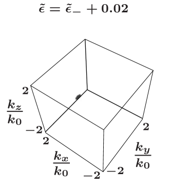
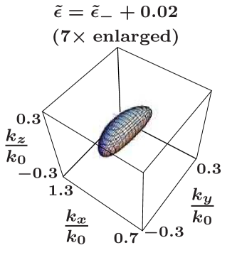
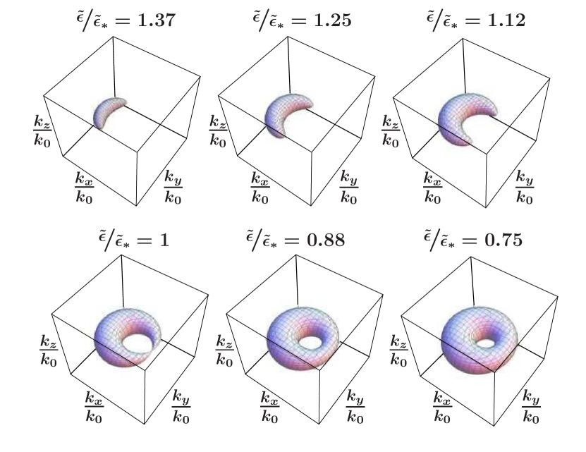
Figure 4: (Color online) (a) Surface of constant energy $E_{\bm{k},-}=\epsilon$ of the lower helicity branch in the ferromagnetic phase just above the lower energy threshold $\tilde{\epsilon}_{-}=-(1+\tilde{p})^{2}$. (b) Same as (a) but enlarged by a factor of seven. (c) Evolution of the constant energy surface for different energies. The scales are the same as in (a). All plots are for $\tilde{p}=0.1$.

With increasing energy the ellipsoid distorts into a bean-shaped surface until the two ends of the bean meet at a critical energy. For higher energies, a hole emerges in the energy surface so that it assumes the topology of a torus. At the critical energy $\epsilon_{\ast}$ where the topology of the energy surface changes the spectral densities have a cusp. From the exact expressions for the spectral densities given in Appendix B it is easy to see that the critical energy is

$$\epsilon_{\ast}=-\epsilon_{0}+\Sigma_{0}+v_{0}p=\epsilon_{-}+2v_{0}p.$$ (74)

A similar transition in the topology of the Fermi surface of metals as a function of external pressure has been discussed a long time ago by Lifshitz Lifshitz60 . Close to such a transition, Lifshitz predicted anomalies in the thermodynamics and the kinetics of the electrons. Therefore we expect that in phases with spontaneous transverse ferromagnetism the kinetics of spin-orbit coupled bosons with energies close to $\epsilon_{\ast}$ is rather unusual.

III.3 Solution of the mean-field equations

For the numerical solution of the above mean-field equations it is useful to introduce the dimensionless density, magnetization, susceptibility, and interaction as follows,

$$\tilde{\rho} = \frac{\rho}{\nu_{0}\epsilon_{0}}=\frac{4\pi\rho}{k_{0}^{3}},$$ (75a)

$$\tilde{M} = \frac{M}{\nu_{0}\epsilon_{0}}=\frac{4\pi M}{k_{0}^{3}},$$ (75b)

$$\tilde{\chi}_{\bot} = \frac{\chi_{\bot}}{\nu_{0}},$$ (75c)

$$\tilde{g}_{\bot} = \nu_{0}g_{\bot}.$$ (75d)

We also introduce the dimensionless energy $\omega=(\epsilon-\epsilon_{-})/\epsilon_{0}$ which is measured relative to the bottom of the lower helicity branch, and define

$$\bar{\nu}_{\lambda}({\omega},\tilde{p}) = \frac{\nu_{\lambda}(\epsilon_{-}+\epsilon_{0}{\omega},k_{0}\tilde{p})}{\nu_{0}}=\tilde{\nu}_{\lambda}\left(-(1+\tilde{p})^{2}+{\omega},\tilde{p}\right),$$

$$\bar{\sigma}_{\lambda}({\omega},\tilde{p}) = \frac{\sigma_{\lambda}(\epsilon_{-}+\epsilon_{0}{\omega},k_{0}\tilde{p})}{\nu_{0}}=\tilde{\sigma}_{\lambda}\left(-(1+\tilde{p})^{2}+{\omega},\tilde{p}\right).$$

Finally, we introduce the dimensionless temperature

$$\tau = T/\epsilon_{0},$$ (78)

and the fugacity

$$z=e^{(\mu-\epsilon_{-})/T}.$$ (79)

With this notation the density equation (51) can be written as

$$\tilde{\rho}=\int_{0}^{\infty}d\omega\sum_{\lambda}\bar{\nu}_{\lambda}(\omega,\tilde{p})\frac{z}{e^{\omega/\tau}-z},$$ (80)

while the self-consistency equation (64) for the dimensionless order parameter $\tilde{p}=p/k_{0}=-\tilde{g}_{\bot}\tilde{M}/2$ becomes

$$\tilde{\chi}_{\bot}(\tau,z,\tilde{p})=-1/\tilde{g}_{\bot},$$ (81)

with

$$\tilde{\chi}_{\bot}=-\frac{1}{2\tau}\int_{0}^{\infty}d\omega\sum_{\lambda}\lambda\bar{\sigma}_{\lambda}(\omega,\tilde{p})\frac{ze^{\omega/\tau}}{[e^{\omega/\tau}-z]^{2}}.$$ (82)

Finally, the dimensionless free energy $f(\tau,\tilde{\rho},\tilde{p})=(\Omega+\mu N)/(V\nu_{0}\epsilon_{0}^{2})$ can be written as

$$f(\tau,\tilde{\rho},\tilde{p}) = \tau\int_{0}^{\infty}d\omega\sum_{\lambda}\bar{\nu}_{\lambda}(\omega,\tilde{p})\ln\left[1-ze^{-\omega/\tau}\right]$$ (83)

$$- \frac{\tilde{g}_{\parallel}}{2}\tilde{\rho}^{2}-\tilde{g}_{\bot}\left(\frac{\tilde{\rho}^{2}}{4}+\tilde{M}^{2}\right)+\tilde{\mu}\tilde{\rho},$$

where $\tilde{\mu}=\mu/\epsilon_{0}$. Note that at constant density we should determine $\mu$ as a function of $\tilde{\rho}$ and $\tilde{p}$.

Let us first discuss the critical temperature $\tau_{c}=T_{c}/\epsilon_{0}$ below which the system exhibits spontaneous transverse ferromagnetism. According to Eq. (81), for a given density $\tilde{\rho}$ the critical temperature is determined by

$$\tilde{\chi}_{\bot}(\tau_{c},z_{c}(\tau_{c},\tilde{\rho}),\tilde{p}=0)=-1/\tilde{g}_{\bot},$$ (84)

where the fugacity $z_{c}(\tau_{c},\tilde{\rho})$ at the critical point is determined by

$$\tilde{\rho}=\int_{0}^{\infty}d\omega\sum_{\lambda}\bar{\nu}_{\lambda}(\omega,0)\frac{z_{c}}{e^{\omega/\tau_{c}}-z_{c}}.$$ (85)

Numerical results for $\tau_{c}$ as a function of $|\tilde{g}_{\bot}|$ for different densities are shown in Fig. 5 (a), while in Fig. 5 (b) we show the critical temperature as a function of density for different values of $|\tilde{g}_{\bot}|$. The numerical results in general are obtained without approximating the spectral densities and choosing $g_{\|}$ such that $\Sigma_{0}$ vanishes.

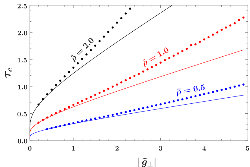
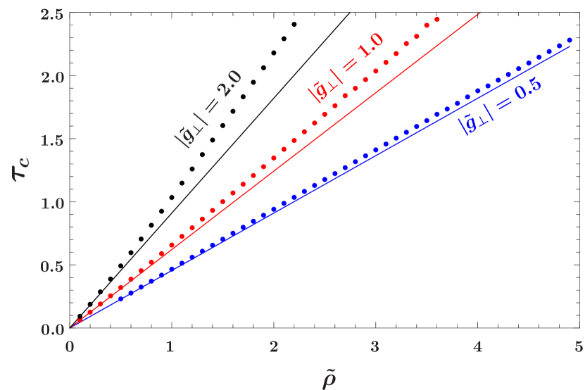
Figure 5: (Color online) (a) Critical temperature for transverse ferromagnetism as a function of the dimensionless coupling constant $|\tilde{g}_{\bot}|$ for three different densities. The dots have been obtained from the numerical solution of the mean-field equations (84) without further approximation, while the solid lines represent the low-temperature approximation (89).  (b) Critical temperature as a function of density for different values of the interaction.

Note that for small $|\tilde{g}_{\bot}|$ the critical temperature approaches zero with infinite slope. In this regime it is easy to obtain an analytic expression for the critical temperature. Assuming that the temperature is small compared with $\epsilon_{0}$ (corresponding to $\tau\ll 1$) we may neglect the contribution of the upper helicity branch and approximate the spectral densities by their leading asymptotics for frequencies close to the bottom of the lower helicity branch given in Eqs. (B14) and (B15). In the symmetric phase where $\tilde{p}=0$ the density equation (80) then reduces to

$$\tilde{\rho}=\int_{0}^{\infty}d\omega\frac{z}{e^{\omega/\tau}-z}=-\tau\ln(1-z).$$ (86)

We conclude that in the regime where the critical temperature $\tau_{c}$ is small compared with unity, the critical fugacity is given by

$$z_{c}=1-e^{-\tilde{\rho}/\tau_{c}}.$$ (87)

For $\tau_{c}\ll\tilde{\rho}$ this is exponentially close to unity, which is a consequence of the finite density of states of the spin-orbit coupled Bose gas close to the bottom of the lower energy branch. To determine the critical temperature as a function of the density, we calculate the transverse susceptibility from Eq. (82) with $\tilde{p}=0$, using the approximation (B15) for the spectral density $\bar{\sigma}_{-}(\omega,0)=\tilde{\sigma}_{-}(-1+\omega,\tilde{p}=0)$ for frequencies close to the bottom of the lower helicity branch,

$$\tilde{\chi}_{\bot} = \frac{1}{4}\int_{0}^{\infty}d\omega\frac{ze^{\omega/\tau}}{[e^{\omega/\tau}-z]^{2}}=\frac{1}{4}\frac{z}{1-z}=\frac{1}{4}\left[e^{\tilde{\rho}/\tau}-1\right].$$

Hence, in the paramagnetic phase the transverse susceptibility becomes exponentially large at low temperatures. As a consequence, for any finite attractive interaction $g_{\bot}<0$, we can find a solution of the self-consistency equation (81) at sufficiently low temperatures. Combining Eqs. (84) and (LABEL:eq:chilow) we obtain for the critical temperature

$$\tau_{c}=\frac{\tilde{\rho}}{\ln\left(1+4/|\tilde{g}_{\bot}|\right)}.$$ (89)

From the derivation of this expression it is clear that Eq. (89) is valid as long as $\tau_{c}\ll 1$, which can always be satisfied for sufficiently small densities. The approximation (89) corresponds to the solid lines in Fig. 5.

Next, let us discuss the low-temperature phase $\tau<\tau_{c}$ with spontaneous transverse ferromagnetism. In Fig. 6 we show the change

$$\Delta f=f(\tau,\tilde{\rho},\tilde{p})-f(\tau,\tilde{\rho},0)$$ (90)

in the dimensionless free energy defined in Eq. (83) as a function of the order parameter $\tilde{M}=2\tilde{p}/|\tilde{g}_{\bot}|$ for three different temperatures.

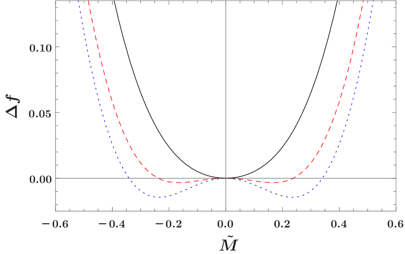
Figure 6: (Color online) Dimensionless free energy $\Delta f$, defined in equation (90), as a function of the dimensionless magnetization $\tilde{M}$ for three different temperatures. $\tau/\tau_{c}=0.9$ (dotted line); $\tau/\tau_{c}=0.95$ (dashed line); $\tau/\tau_{c}=1.1$ (solid line). For all plots we have used $|\tilde{g}_{\bot}|=5$ and $\tilde{\rho}=1$.

For $\tau<\tau_{c}$ the free energy continuously develops two degenerate minima, corresponding to the Hartree-Fock solutions $\pm\tilde{M}$. The phase transition to the magnetic state is therefore second order. The transverse magnetization as a function of temperature for three different densities, obtained numerically, is shown in Fig. 7.

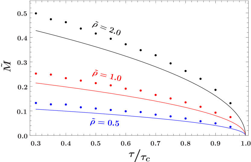
Figure 7: (Color online) Transverse magnetization as a function of temperature. The plots are for $|\tilde{g}_{\bot}|=1$. The dots are obtained numerically, while the solid lines correspond to the analytic result (91) which is only valid for $\tau_{c}-\tau\ll\tau_{c}\ll 1$.

In the regime where $\tau_{c}\ll 1$ the behavior of the magnetization for temperatures close to the critical temperature can be calculated analytically, as shown in Appendix C. We find

$$\tilde{M}\sim\frac{\tilde{\rho}}{\sqrt{\left(8+\frac{3}{2}|\tilde{g}_{\bot}|\right)\ln[1+\frac{4}{|\tilde{g}_{\bot}|}]}}\sqrt{\frac{\tau_{c}-\tau}{\tau_{c}}}.$$ (91)

The reason we obtain the usual mean-field exponent $\beta=1/2$ is of course related to the fact that our calculation is based on the Hartree-Fock approximation.

IV Summary and conclusions

In summary, we have shown that in the spinor Bose gas with Rashba-type spin-orbit coupling an arbitrarily weak attractive interaction between bosons with opposite spin triggers a ferromagnetic instability for temperatures below some finite temperature $T_{c}$ if the density of the bosons is fixed. Note that spontaneous ferromagnetism in electronic systems usually appears only if the relevant interaction exceeds a finite threshold Moriya85 . The fact that in the spinor Bose gas such a threshold does not exist is related to the singularity of the Bose function for small energies in combination with the finite density of states in the non-magnetic phase due to the spin-orbit coupling of the Rashba-type. Because for $T<T_{c}$, the density of states exhibits the usual $\sqrt{\omega}$-behavior at low energies, at some temperature below $T_{c}$ the bosons eventually condense into the single-particle state with the lowest momentum $\bm{k}_{0}$, which is unique in the ferromagnetic phase. In the weak coupling regime, we may estimate the critical temperature for BEC by using the critical temperature for free bosons with anisotropic dispersion given by Eq. (73),

$$T_{\rm BEC} = \frac{2\pi}{m}\left(\frac{\rho}{\zeta(3/2)}\right)^{2/3}\left(\frac{p}{k_{0}+p}\right)^{1/3}$$ (92)

$$= \frac{2\pi}{m}\left(\frac{\rho}{\zeta(3/2)}\right)^{2/3}\left(\frac{|g_{\bot}|M}{k_{0}^{2}/m+|g_{\bot}|M}\right)^{1/3}.\hskip 28.45274pt$$

For consistency, we should require that $T_{\rm BEC}<T_{c}$, which is satisfied at weak coupling where $p\ll k_{0}$. We thus conclude that the ground state of the spinor Bose gas with Rashba spin-orbit coupling and attractive interaction $g_{\bot}<0$ is a ferromagnetic Bose-Einstein condensate.

In principle, an attractive interaction $g_{\bot}<0$ could also trigger an instability in the particle-particle channel, leading to a pair condensate at low temperatures. However, as shown in Appendix D, at least for sufficiently low densities the ferromagnetic instability has a higher critical temperature if the relevant coupling constants have the same order of magnitude.

Let us also point out that the constant $g_{\bot}$ in our mean-field calculation should be considered as an effective low-energy interaction in the opposite-spin particle-hole channel. This interaction includes renormalization effects from high-energy fluctuations in all channels, so that it is in principle possible that the effective low-energy coupling is attractive even if we start from a repulsive bare interaction. Note that recently Gopalakrishnan et al. Gopalakrishnan11 performed a momentum shell renormalization group calculation for the spin-orbit coupled Bose gas whose dispersion exhibits a minimum on a circle in momentum space; at finite temperature they found evidence for an attractive renormalized coupling in the particle-particle channel, although the corresponding bare interaction is repulsive, suggesting an instability towards pair condensation. However, a proper renormalization group calculation of the effective low-energy coupling of the spinor Bose gas with Rashba-type spin-orbit coupling, taking high-energy fluctuations in all channels and all relevant and marginal couplings consistently into account, still remains to be done. Given the fact that the system belongs to the Brazovskii universality class, the rescaling step in the renormalization group transformation is non-trivial and all two-body scattering processes describing particles with momenta on the low-energy manifold are marginal and should be retained. It should be advantageous to use the well developed machinery of the functional renormalization group Kopietz10 ; Kopietz01 ; Metzner12 to carry out such a calculation.

APPENDIX A: Interactions in the helicity basis

In this appendix we explicitly give the interaction part of the boson Hamiltonian (4) in the helicity basis. For simplicity, we assume momentum independent bare interactions, see Eq. (6). To transform the interaction from the spin basis to the helicity basis, it is useful to introduce the notation $a_{\bm{k}}=a_{\bm{k}-}$ and $b_{\bm{k}}=e^{-i\varphi_{\bm{k}}}a_{\bm{k}+}$, so that our transformation (12) to the helicity basis can be written as

$$a_{\bm{k}\uparrow} = \frac{1}{\sqrt{2}}\left[a_{\bm{k}-}-e^{-i\varphi_{\bm{k}}}a_{\bm{k}+}\right]=\frac{1}{\sqrt{2}}\left[a_{\bm{k}}-b_{\bm{k}}\right],$$ (A1)

$$a_{\bm{k}\downarrow} = \frac{1}{\sqrt{2}}\left[e^{i\varphi_{\bm{k}}}a_{\bm{k}-}+a_{\bm{k}+}\right]=\frac{e^{i\varphi_{\bm{k}}}}{\sqrt{2}}\left[a_{\bm{k}}+b_{\bm{k}}\right].$$ (A2)

Defining the coupling constants $g_{\uparrow}$, $g_{\downarrow}$ and $g_{\bot}$ as in Eq. (6), we find that in the helicity basis the interaction part (7) of our Hamiltonian can be written as

$${\cal{H}}_{\rm int} = \frac{1}{V}\sum_{\bm{k}_{1}^{\prime}\bm{k}_{2}^{\prime}\bm{k}_{2}\bm{k}_{1}}\delta_{\bm{k}_{1}^{\prime}+\bm{k}_{2}^{\prime},\bm{k}_{2}+\bm{k}_{1}}\Bigl{\{}\frac{1}{(2!)^{2}}\Bigl{[}\Gamma_{0}^{\bar{a}\bar{a}aa}(1^{\prime},2^{\prime};{2},1)a^{\dagger}_{1^{\prime}}a^{\dagger}_{2^{\prime}}a_{2}a_{1}+\Gamma_{0}^{\bar{b}\bar{b}bb}(1^{\prime},2^{\prime};{2},1)b^{\dagger}_{1^{\prime}}b^{\dagger}_{2^{\prime}}b_{2}b_{1}$$ (A3)

$$\hskip 130.88268pt+\Gamma_{0}^{\bar{a}\bar{a}bb}(1^{\prime},2^{\prime};{2},1)a^{\dagger}_{1^{\prime}}a^{\dagger}_{2^{\prime}}b_{2}b_{1}+\Gamma_{0}^{\bar{b}\bar{b}aa}(1^{\prime},2^{\prime};{2},1)b^{\dagger}_{1^{\prime}}b^{\dagger}_{2^{\prime}}a_{2}a_{1}\Bigr{]}$$

$$\hskip 113.81102pt+\frac{1}{2!}\Bigl{[}\Gamma_{0}^{\bar{a}\bar{a}ab}(1^{\prime},2^{\prime};{2},1)a^{\dagger}_{1^{\prime}}a^{\dagger}_{2^{\prime}}a_{2}b_{1}+\Gamma_{0}^{\bar{b}\bar{b}ba}(1^{\prime},2^{\prime};{2},1)b^{\dagger}_{1^{\prime}}b^{\dagger}_{2^{\prime}}b_{2}a_{1}$$

$$\hskip 130.88268pt+\Gamma_{0}^{\bar{b}\bar{a}aa}(1^{\prime},2^{\prime};{2},1)b^{\dagger}_{1^{\prime}}a^{\dagger}_{2^{\prime}}a_{2}a_{1}+\Gamma_{0}^{\bar{a}\bar{b}bb}(1^{\prime},2^{\prime};{2},1)a^{\dagger}_{1^{\prime}}b^{\dagger}_{2^{\prime}}b_{2}b_{1}\Bigr{]}$$

$$\hskip 113.81102pt+\Gamma_{0}^{\bar{a}\bar{b}ba}(1^{\prime},2^{\prime};{2},1)a^{\dagger}_{1^{\prime}}b^{\dagger}_{2^{\prime}}b_{2}a_{1}\Bigr{\}}$$

$$= \frac{1}{V}\sum_{\bm{k}_{1}^{\prime}\bm{k}_{2}^{\prime}\bm{k}_{2}\bm{k}_{1}}\delta_{\bm{k}_{1}^{\prime}+\bm{k}_{2}^{\prime},\bm{k}_{2}+\bm{k}_{1}}\Bigl{\{}\frac{1}{(2!)^{2}}U_{1}(\bm{k}_{1}^{\prime},\bm{k}_{2}^{\prime};\bm{k}_{2},\bm{k}_{1})[a^{\dagger}_{1^{\prime}}a^{\dagger}_{2^{\prime}}a_{2}a_{1}+b^{\dagger}_{1^{\prime}}b^{\dagger}_{2^{\prime}}b_{2}b_{1}]$$

$$\hskip 116.6563pt+\frac{1}{(2!)^{2}}U_{2}(\bm{k}_{1}^{\prime},\bm{k}_{2}^{\prime};\bm{k}_{2},\bm{k}_{1})[a^{\dagger}_{1^{\prime}}a^{\dagger}_{2^{\prime}}b_{2}b_{1}+b^{\dagger}_{1^{\prime}}b^{\dagger}_{2^{\prime}}a_{2}a_{1}]$$

$$\hskip 116.6563pt+\frac{1}{2!}U_{3}(\bm{k}_{1}^{\prime},\bm{k}_{2}^{\prime};\bm{k}_{2};\bm{k}_{1})[a^{\dagger}_{1^{\prime}}a^{\dagger}_{2^{\prime}}a_{2}b_{1}+b^{\dagger}_{1^{\prime}}b^{\dagger}_{2^{\prime}}b_{2}a_{1}]$$

$$\hskip 116.6563pt+\frac{1}{2!}U_{4}(\bm{k}_{1}^{\prime};\bm{k}_{2}^{\prime};\bm{k}_{2},\bm{k}_{1})[b^{\dagger}_{1^{\prime}}a^{\dagger}_{2^{\prime}}a_{2}a_{1}+a^{\dagger}_{1^{\prime}}b^{\dagger}_{2^{\prime}}b_{2}b_{1}]$$

$$\hskip 116.6563pt+U_{5}(\bm{k}_{1}^{\prime};\bm{k}_{2}^{\prime};\bm{k}_{2};\bm{k}_{1})a^{\dagger}_{1^{\prime}}b^{\dagger}_{2^{\prime}}b_{2}a_{1}\Bigr{\}}.\hskip 19.91692pt$$

The properly symmetrized interaction vertices are

$$\Gamma_{0}^{\bar{a}\bar{a}aa}(1^{\prime},2^{\prime};{2},1)=\Gamma_{0}^{\bar{b}\bar{b}bb}(1^{\prime},2^{\prime};{2},1) \equiv U_{1}(\bm{k}_{1}^{\prime},\bm{k}_{2}^{\prime};\bm{k}_{2},\bm{k}_{1})$$ (A4a)

$$= \frac{g_{\uparrow}}{2}+\frac{g_{\downarrow}}{2}e^{-i(\varphi_{1^{\prime}}+\varphi_{2^{\prime}}-\varphi_{2}-\varphi_{1})}+\frac{g_{\bot}}{4}(e^{-i\varphi_{1^{\prime}}}+e^{-i\varphi_{2^{\prime}}})(e^{i\varphi_{1}}+e^{i\varphi_{2}}),$$

$$\Gamma_{0}^{\bar{a}\bar{a}bb}(1^{\prime},2^{\prime};{2},1)=\Gamma_{0}^{\bar{b}\bar{b}aa}(1^{\prime},2^{\prime};{2},1) \equiv U_{2}(\bm{k}_{1}^{\prime},\bm{k}_{2}^{\prime};\bm{k}_{2},\bm{k}_{1})$$ (A4b)

$$= \frac{g_{\uparrow}}{2}+\frac{g_{\downarrow}}{2}e^{-i(\varphi_{1^{\prime}}+\varphi_{2^{\prime}}-\varphi_{2}-\varphi_{1})}-\frac{g_{\bot}}{4}(e^{-i\varphi_{1^{\prime}}}+e^{-i\varphi_{2^{\prime}}})(e^{i\varphi_{1}}+e^{i\varphi_{2}}),\hskip 19.91692pt$$

$$\Gamma_{0}^{\bar{a}\bar{a}ab}(1^{\prime},2^{\prime};{2},1)=\Gamma_{0}^{\bar{b}\bar{b}ba}(1^{\prime},2^{\prime};{2},1) \equiv U_{3}(\bm{k}_{1}^{\prime},\bm{k}_{2}^{\prime};\bm{k}_{2};\bm{k}_{1})$$ (A4c)

$$= -\frac{g_{\uparrow}}{2}+\frac{g_{\downarrow}}{2}e^{-i(\varphi_{1^{\prime}}+\varphi_{2^{\prime}}-\varphi_{2}-\varphi_{1})}+\frac{g_{\bot}}{4}(e^{-i\varphi_{1^{\prime}}}+e^{-i\varphi_{2^{\prime}}})(e^{i\varphi_{1}}-e^{i\varphi_{2}}),\hskip 19.91692pt$$

$$\Gamma_{0}^{\bar{b}\bar{a}aa}(1^{\prime},2^{\prime};{2},1)=\Gamma_{0}^{\bar{a}\bar{b}bb}(1^{\prime},2^{\prime};{2},1) \equiv U_{4}(\bm{k}_{1}^{\prime};\bm{k}_{2}^{\prime};\bm{k}_{2},\bm{k}_{1})$$ (A4d)

$$= -\frac{g_{\uparrow}}{2}+\frac{g_{\downarrow}}{2}e^{-i(\varphi_{1^{\prime}}+\varphi_{2^{\prime}}-\varphi_{2}-\varphi_{1})}+\frac{g_{\bot}}{4}(e^{-i\varphi_{1^{\prime}}}-e^{-i\varphi_{2^{\prime}}})(e^{i\varphi_{1}}+e^{i\varphi_{2}}),\hskip 19.91692pt$$

$$\Gamma_{0}^{\bar{a}\bar{b}ba}(1^{\prime},2^{\prime};{2},1) \equiv U_{5}(\bm{k}_{1}^{\prime};\bm{k}_{2}^{\prime};\bm{k}_{2};\bm{k}_{1})$$ (A4e)

$$= \frac{g_{\uparrow}}{2}+\frac{g_{\downarrow}}{2}e^{-i(\varphi_{1^{\prime}}+\varphi_{2^{\prime}}-\varphi_{2}-\varphi_{1})}+\frac{g_{\bot}}{4}(e^{-i\varphi_{1^{\prime}}}-e^{-i\varphi_{2^{\prime}}})(e^{i\varphi_{1}}-e^{i\varphi_{2}}).\hskip 19.91692pt$$

The parametrization of the vertices in terms of five functions $U_{1},\ldots,U_{5}$ is similar to the parametrization used by Ozawa and Baym Ozawa11 ; however, we find it convenient to introduce slightly different numerical prefactors in the second line of Eq. (A3) in order to simplify the combinatorial factors due the permutation symmetries of the vertices in higher order calculations. Note that the interaction vertices are invariant under arbitrary rotations around the $z$ axis, corresponding to a shift $\varphi_{\bm{k}}\rightarrow\varphi_{\bm{k}}+\alpha$ in all angles.

APPENDIX B: Spectral densities

In this appendix we discuss the dimensionless scaling functions $\tilde{\nu}_{\lambda}(\tilde{\epsilon},\tilde{p})$ and $\tilde{\sigma}_{\lambda}(\tilde{\epsilon},\tilde{p})$ which are defined by writing the density of states and the weighted density of states in the scaling form (67, 68). The scaling function $\tilde{\nu}_{\lambda}(\tilde{\epsilon},\tilde{p})$ for the density of states can be written as

$$\tilde{\nu}_{\lambda}(\tilde{\epsilon},\tilde{p}) = \Theta(\tilde{\epsilon})\left\{\frac{\sqrt{\tilde{\epsilon}}}{\pi}+\int_{0}^{2\pi}\frac{d\varphi}{2\pi}(\tilde{p}\cos\varphi-\lambda)\left[\frac{1}{2}+\frac{1}{\pi}\arctan\left(\frac{\tilde{p}\cos\varphi-\lambda}{\sqrt{\tilde{\epsilon}}}\right)\right]\right\}$$ (B1)

$$+ \Theta(-\tilde{\epsilon})\int_{0}^{2\pi}\frac{d\varphi}{2\pi}(\tilde{p}\cos\varphi-\lambda)\Theta(\tilde{p}\cos\varphi-\lambda-\sqrt{-\tilde{\epsilon}}).$$

Recall that in Eqs. (67) and (68) the dimensionless variables $\tilde{\epsilon}$ and $\tilde{p}$ represent

$$\tilde{\epsilon}=\frac{\epsilon-\Sigma_{0}-\frac{p^{2}}{2m}}{\epsilon_{0}},\qquad\tilde{p}=\frac{p}{k_{0}}.$$ (B2)

For negative $\tilde{\epsilon}$ the angular integration in Eq. (B1) can be done analytically. For the lower energy branch ($\lambda=-1$) we obtain

$$\tilde{\nu}_{-}(\tilde{\epsilon},\tilde{p}) = \Theta(1-\sqrt{-\tilde{\epsilon}}-\tilde{p})+\Theta(\tilde{p}-|1-\sqrt{-\tilde{\epsilon}}|)\frac{1}{\pi}\left[\arccos\left(\frac{\sqrt{-\tilde{\epsilon}}-1}{\tilde{p}}\right)+\sqrt{\tilde{p}^{2}-(1-\sqrt{-\tilde{\epsilon}})^{2}}\right],\;\;\;\mbox{for $\tilde{\epsilon}<0$}.$$ (B3)

The scaling function for the weighted density of states $\tilde{\sigma}_{\lambda}(\tilde{\epsilon},\tilde{p})$, can be written as

$$\tilde{\sigma}_{\lambda}(\tilde{\epsilon},\tilde{p}) = \Theta(\tilde{\epsilon})\int_{0}^{2\pi}\frac{d\varphi}{2\pi}\frac{\sin^{2}\varphi}{2}\left\{\left[3(\tilde{p}\cos\varphi-\lambda)^{2}+\tilde{\epsilon}\right]\left[\frac{1}{2}+\frac{1}{\pi}\arctan\left(\frac{\tilde{p}\cos\varphi-\lambda}{\sqrt{\tilde{\epsilon}}}\right)\right]+\frac{3\sqrt{\tilde{\epsilon}}}{\pi}(\tilde{p}\cos\varphi-\lambda)\right\}$$ (B4)

$$+ \Theta(-\tilde{\epsilon})\int_{0}^{2\pi}\frac{d\varphi}{2\pi}\frac{\sin^{2}\varphi}{2}\left[3(\tilde{p}\cos\varphi-\lambda)^{2}+\tilde{\epsilon}\right]\Theta(\tilde{p}\cos\varphi-\lambda-\sqrt{-\tilde{\epsilon}}).$$

For negative $\tilde{\epsilon}$ the angular integration can again be performed analytically. For the lower energy branch ($\lambda=-1$) we obtain

$$\tilde{\sigma}_{-}(\tilde{\epsilon},\tilde{p}) = \Theta(1-\sqrt{-\tilde{\epsilon}}-\tilde{p})\frac{1}{4}\left(3+\tilde{\epsilon}+\frac{3}{4}\tilde{p}^{2}\right)+\Theta(\tilde{p}-|1-\sqrt{-\tilde{\epsilon}}|)\frac{1}{4\pi}\Biggl{[}\left(3+\tilde{\epsilon}+\frac{3}{4}\tilde{p}^{2}\right)\arccos\left(\frac{\sqrt{-\tilde{\epsilon}}-1}{\tilde{p}}\right)$$ (B5)

$$+\sqrt{\tilde{p}^{2}-(1-\sqrt{-\tilde{\epsilon}})^{2}}\left(\frac{(1+\tilde{\epsilon})(1+\sqrt{-\tilde{\epsilon}})}{2\tilde{p}^{2}}+\frac{13+3\sqrt{-\tilde{\epsilon}}}{4}\right)\Biggr{]},\;\;\;\mbox{for $\tilde{\epsilon}<0$}.$$

Plots of the above scaling functions are shown in Fig. 3. The asymptotic behavior slightly above the lower threshold $\tilde{\epsilon}_{-}=-(1+\tilde{p})^{2}$ is,

$$\tilde{\nu}_{-}(\tilde{\epsilon},\tilde{p}) \sim \frac{\sqrt{1+\tilde{p}}}{\pi}\sqrt{\frac{\tilde{\epsilon}+(1+\tilde{p})^{2}}{\tilde{p}}},$$ (B6)

$$\tilde{\sigma}_{-}(\tilde{\epsilon},\tilde{p}) \sim \frac{\sqrt{1+\tilde{p}}}{3\pi}\left[\frac{\tilde{\epsilon}+(1+\tilde{p})^{2}}{\tilde{p}}\right]^{3/2}.$$ (B7)

To discuss the thermodynamics close to the critical point, we need the expansion of the density of states and the weighted density of states for small $\tilde{p}=p/k_{0}$ to order $\tilde{p}^{2}$. We obtain

$$\frac{{\nu}_{\lambda}(\epsilon,p)}{\nu_{0}}=\tilde{\nu}_{\lambda}^{(0)}\left(\frac{\epsilon-\Sigma_{0}}{\epsilon_{0}}\right)+\tilde{p}^{2}\tilde{\nu}_{\lambda}^{(2)}\left(\frac{\epsilon-\Sigma_{0}}{\epsilon_{0}}\right)+{\cal{O}}(\tilde{p}^{4}),$$ (B8)

where

$$\tilde{\nu}_{\lambda}^{(0)}(\tilde{\epsilon}) = \Theta(\tilde{\epsilon})\left[\frac{\sqrt{\tilde{\epsilon}}}{\pi}-\frac{\lambda}{2}+\frac{1}{\pi}\arctan\left(\frac{1}{\sqrt{\tilde{\epsilon}}}\right)\right]$$ (B9)

$$+ \Theta(-\tilde{\epsilon})\delta_{\lambda,-1}\Theta(1-\sqrt{-\tilde{\epsilon}}),$$

$$\tilde{\nu}_{\lambda}^{(2)}(\tilde{\epsilon}) = -\frac{\Theta(\tilde{\epsilon})}{2}\frac{\sqrt{\tilde{\epsilon}}}{\pi(1+\tilde{\epsilon})^{2}}$$ (B10)

$$+ \frac{\Theta(-\tilde{\epsilon})}{4}\delta_{\lambda,-1}\delta^{\prime}(1-\sqrt{-\tilde{\epsilon}}),$$

and $\delta^{\prime}(x)=\frac{d}{dx}\delta(x)$ is the derivative of the $\delta$-function with respect to its argument. The order parameter expansion of the weighted density of states is

$$\frac{\sigma_{\lambda}(\epsilon,p)}{\nu_{0}}=\tilde{\sigma}_{\lambda}^{(0)}\left(\frac{\epsilon-\Sigma_{0}}{\epsilon_{0}}\right)+\tilde{p}^{2}\tilde{\sigma}_{\lambda}^{(2)}\left(\frac{\epsilon-\Sigma_{0}}{\epsilon_{0}}\right)+{\cal{O}}(\tilde{p}^{4}),$$ (B11)

with

$$\tilde{\sigma}_{\lambda}^{(0)}(\tilde{\epsilon}) = \frac{\Theta(\tilde{\epsilon})}{4}\left\{(3+\tilde{\epsilon})\left[\frac{1}{2}-\frac{\lambda}{\pi}\arctan\left(\frac{1}{\sqrt{\tilde{\epsilon}}}\right)\right]-\lambda\frac{3\sqrt{\tilde{\epsilon}}}{\pi}\right\}$$ (B12)

$$+ \frac{\Theta(-\tilde{\epsilon})}{4}\delta_{\lambda,-1}\Theta(1-\sqrt{-\tilde{\epsilon}})(3+\tilde{\epsilon}),$$

$$\tilde{\sigma}_{\lambda}^{(2)}(\tilde{\epsilon}) = \frac{\Theta(\tilde{\epsilon})}{16}\left[\frac{\lambda\sqrt{\tilde{\epsilon}}(1-\tilde{\epsilon})}{\pi(1+\tilde{\epsilon})^{2}}-\frac{1}{2}+\frac{\lambda}{\pi}\arctan\left(\frac{1}{\sqrt{\tilde{\epsilon}}}\right)\right]$$ (B13)

$$+ \frac{\Theta(-\tilde{\epsilon})}{16}\delta_{\lambda,-1}\Bigl{[}-\Theta(1-\sqrt{-\tilde{\epsilon}})+2\delta(1-\sqrt{-\tilde{\epsilon}})$$

$$\hskip 51.21495pt+\frac{3+\tilde{\epsilon}}{2}\delta^{\prime}(1-\sqrt{-\tilde{\epsilon}})\Bigr{]}.$$

At low temperatures only the leading asymptotics of these functions close to the bottom of the lower energy branch is relevant. Shifting the dimensionless energy as $\tilde{\epsilon}=-1+\omega$, we may approximate for $|\omega|\ll 1$,

$$\tilde{\nu}_{-}^{(0)}(-1+\omega) \approx \Theta(\omega),$$ (B14)

$$\tilde{\sigma}_{-}^{(0)}(-1+\omega) \approx \frac{\Theta(\omega)}{2},$$ (B15)

$$\tilde{\nu}_{-}^{(2)}(-1+\omega) \approx \frac{1}{4}\delta^{\prime}(1-\sqrt{1-\omega})\approx\delta^{\prime}(\omega),$$ (B16)

$$\tilde{\sigma}_{-}^{(2)}(-1+\omega) \approx \frac{1}{16}\left[-\Theta(\omega)+2\delta(\omega)+4\delta^{\prime}(\omega)\right],\hskip 19.91692pt$$ (B17)

where we have used $\delta^{\prime}(a\omega)=a^{-2}\delta^{\prime}(\omega)$ and $\omega\delta^{\prime}(\omega)=-\delta(\omega)$.

APPENDIX C: Order parameter expansion

For temperatures slightly below the critical temperature the order parameter $\tilde{p}=|\tilde{g}_{\bot}|\tilde{M}/2$ is small so that we may expand all quantities to second order in powers of $\tilde{p}$. Having expressed all quantities in terms of the spectral densities ${\nu}_{\lambda}(\epsilon,p)$ and $\sigma_{\lambda}(\epsilon,p)$, we use the order parameter expansion of these, given in Eqs. (B8, B11), to generate the corresponding expansion of any other quantity. Using the density equation (80) we obtain for the chemical potential

$$\mu=\mu_{0}+\mu_{2}\tilde{p}^{2}+{\cal{O}}(\tilde{p}^{4}),$$ (C1)

where the chemical potential for vanishing order parameter is determined by

$$\tilde{\rho}=\int_{-\infty}^{\infty}d\tilde{\epsilon}\sum_{\lambda}\tilde{\nu}^{(0)}_{\lambda}(\tilde{\epsilon})n_{0}(\tilde{\epsilon}),$$ (C2)

with

$$n_{0}(\tilde{\epsilon})=\frac{1}{e^{(\tilde{\epsilon}+\tilde{\Sigma}_{0}-\tilde{\mu}_{0})/\tau}-1}.$$ (C3)

Here $\tilde{\Sigma}_{0}=\Sigma_{0}/\epsilon_{0}$ and $\tilde{\mu}_{0}=\mu_{0}/\epsilon_{0}$. The leading correction to the chemical potential in the symmetry broken phase is

$$\frac{\mu_{2}}{T}=\frac{\tilde{\mu}_{2}}{\tau}=\frac{\int_{-\infty}^{\infty}d\tilde{\epsilon}\sum_{\lambda}\tilde{\nu}^{(2)}_{\lambda}(\tilde{\epsilon})n_{0}(\tilde{\epsilon})}{\int_{-\infty}^{\infty}d\tilde{\epsilon}\sum_{\lambda}\tilde{\nu}^{(0)}_{\lambda}(\tilde{\epsilon})n_{0}(\tilde{\epsilon})[n_{0}(\tilde{\epsilon})+1]}.$$ (C4)

The corresponding expansion of the susceptibility $\tilde{\chi}_{\bot}$ defined in Eq. (82) is

$$\tilde{\chi}_{\bot}=\tilde{\chi}_{\bot}^{(0)}+\tilde{p}^{2}\tilde{\chi}_{\bot}^{(2)}+{\cal{O}}(\tilde{p}^{4}),$$ (C5)

with

$$\tilde{\chi}_{\bot}^{(0)}=-\frac{1}{2\tau}\int_{-\infty}^{\infty}d\tilde{\epsilon}\sum_{\lambda}\lambda\tilde{\sigma}^{(0)}_{\lambda}(\tilde{\epsilon})n_{0}(\tilde{\epsilon})[n_{0}(\tilde{\epsilon})+1],$$ (C6)

and

$$\tilde{\chi}_{\bot}^{(2)} = -\frac{1}{2\tau}\int_{-\infty}^{\infty}d\tilde{\epsilon}\sum_{\lambda}\lambda\biggl{\{}\tilde{\sigma}^{(2)}_{\lambda}(\tilde{\epsilon})n_{0}(\tilde{\epsilon})[n_{0}(\tilde{\epsilon})+1]$$ (C7)

$$- \frac{\tilde{\mu}_{2}}{\tau}\tilde{\sigma}^{(0)}_{\lambda}(\tilde{\epsilon})n_{0}(\tilde{\epsilon})[n_{0}(\tilde{\epsilon})+1][2n_{0}(\tilde{\epsilon})+1]\biggr{\}}.$$

And finally, the expansion of the dimensionless free energy defined in Eq. (83) is

$$f\equiv\frac{\Omega+\mu N}{V\nu_{0}\epsilon_{0}^{2}}=f_{0}+\tilde{p}^{2}f_{2}+{\cal{O}}(\tilde{p}^{4}),$$ (C8)

with

$$f_{0} = \tau\int_{-\infty}^{\infty}d\tilde{\epsilon}\sum_{\lambda}\tilde{\nu}^{(0)}_{\lambda}(\tilde{\epsilon})\ln\left[1-e^{-(\tilde{\epsilon}+\tilde{\Sigma}_{0}-\tilde{\mu}_{0})/\tau}\right]$$ (C9)

$$- \frac{1}{2}\left[\tilde{g}_{\parallel}+\frac{\tilde{g}_{\bot}}{2}\right]\tilde{\rho}^{2}+\tilde{\mu}_{0}\tilde{\rho},$$

$$f_{2} = \frac{4}{-g_{\bot}}+\tau\int_{-\infty}^{\infty}d\tilde{\epsilon}\sum_{\lambda}\tilde{\nu}^{(2)}_{\lambda}(\tilde{\epsilon})\ln\left[1-e^{-(\tilde{\epsilon}+\tilde{\Sigma}_{0}-\tilde{\mu}_{0})/\tau}\right].$$

In the low-temperature regime $\tau\ll 1$ the above expressions can be evaluated analytically because it is then allowed to substitute the leading asymptotics of the spectral densities for energies close to the bottom of the lower branch given in Eqs. (B14–B17). The zeroth order chemical potential and the corresponding fugacity $z_{0}$ are then given by

$$z_{0}=e^{(\tilde{\mu}_{0}-\tilde{\Sigma}_{0}+1)/\tau}=1-e^{-\tilde{\rho}/\tau},$$ (C11)

while the correction to the chemical potential is

$$\tilde{\mu}_{2}=\frac{1}{\tau(1-z_{0})}=\frac{e^{\tilde{\rho}/\tau}}{\tau}.$$ (C12)

The zeroth order susceptibility $\tilde{\chi}_{\bot}^{(0)}$ is given by the right-hand side of Eq. (LABEL:eq:chilow), while the leading correction is

$$\tilde{\chi}_{\bot}^{(2)}\approx-\frac{z_{0}(3+z_{0})}{8\tau^{2}(1-z_{0})^{3}}.$$ (C13)

The order parameter close to the critical point shows the usual mean-field behavior,

$$\tilde{p}\sim(1-z_{0})\sqrt{\frac{2\tilde{\rho}\tau_{c}}{z_{0}(3+z_{0})}}\sqrt{\frac{\tau_{c}-\tau}{\tau_{c}}}.$$ (C14)

At the critical temperature we may write

$$1-z_{0}=e^{-\tilde{\rho}/\tau_{c}}=\frac{1}{1+\frac{4}{|\tilde{g}_{\bot}|}},$$ (C15)

so that we arrive at Eq. (91) for the transverse magnetization $\tilde{M}=2\tilde{p}/|\tilde{g}_{\bot}|$. Finally, the leading coefficient in the expansion of the free energy is

$$f_{0}=-\tau^{2}{\rm Li}_{2}(z_{0})-\frac{1}{2}\left[\tilde{g}_{\parallel}+\frac{\tilde{g}_{\bot}}{2}\right]\tilde{\rho}^{2}+\tilde{\mu}_{0}\tilde{\rho},$$ (C16)

where ${\rm Li}_{2}(z_{0})$ is the polylogarithm. The coefficient of the term proportional to $\tilde{p}^{2}$ is

$$f_{2}=-\frac{4}{\tilde{g}_{\bot}}-\frac{z_{0}}{1-z_{0}}=4\left[\frac{1}{|\tilde{g}_{\bot}|}-\tilde{\chi}_{\bot}^{(0)}\right].$$ (C17)

Note that for $\tau<\tau_{c}$ the right-hand side of this expression is negative, so that in the ferromagnetic phase the system indeed gains energy.

APPENDIX D: Pair condensation

For attractive $g_{\bot}$ the system can also exhibit a pairing instability which competes with the ferromagnetic instability discussed in the main text. In this appendix we show however that, at least for sufficiently low densities, the ferromagnetic instability is dominant.

If we decouple the interaction in the particle-particle channel, we obtain the mean-field Hamiltonian

$${\cal{H}}_{\rm MF}-\mu{\cal{N}} = \sum_{\bm{k}}\Bigl{[}(E_{\bm{k}-}-\mu)a^{\dagger}_{\bm{k}}a_{\bm{k}}+(E_{\bm{k}+}-\mu)b^{\dagger}_{\bm{k}}b_{\bm{k}}$$ (D1)

$$+\bar{\chi}_{0}e^{i\varphi_{\bm{k}}}a_{-\bm{k}}b_{\bm{k}}+\chi_{0}e^{-i\varphi_{\bm{k}}}b^{\dagger}_{\bm{k}}a^{\dagger}_{-\bm{k}}\Bigr{]}+\frac{V}{|g_{\bot}|}|\chi_{0}|^{2}.$$

In general, the boson-pairing order parameter $\chi_{0}=|\chi_{0}|e^{i\alpha}$ is complex, but all phases can be eliminated by setting $\tilde{a}_{\bm{k}}=e^{i\varphi_{\bm{k}}-i\alpha}a_{\bm{k}}$. The Hamiltonian can then be diagonalized by means of a Bogoliubov transformation,

$$\left(\begin{array}[]{c}\tilde{a}_{\bm{k}}\\ b_{\bm{k}}^{\dagger}\end{array}\right)=\left(\begin{array}[]{cc}u_{\bm{k}}^{\ast}&-v_{\bm{k}}^{\ast}\\ -v_{\bm{k}}&u_{\bm{k}}\end{array}\right)\left(\begin{array}[]{c}{\alpha}_{\bm{k}}\\ \beta_{\bm{k}}^{\dagger}\end{array}\right),$$ (D2)

with

$$u_{\bm{k}} = \sqrt{\frac{\xi_{\bm{k}}+\omega_{\bm{k}}}{2\omega_{\bm{k}}}},\;\;\;v_{\bm{k}}=\sqrt{\frac{\xi_{\bm{k}}-\omega_{\bm{k}}}{2\omega_{\bm{k}}}},$$ (D3)

where

$$\xi_{\bm{k}} = \frac{\bm{k}^{2}}{2m}-\mu,\;\;\;\omega_{\bm{k}}=\sqrt{\xi_{\bm{k}}^{2}-|\chi_{0}|^{2}}.$$ (D4)

The corresponding grand canonical potential is

$$\Omega_{\rm MF} = T\sum_{\bm{k}\lambda}\ln\left[1-e^{-\beta(\omega_{\bm{k}}+\lambda v_{0}|\bm{k}_{\bot}|)}\right]$$ (D5)

$$+ \sum_{\bm{k}}(\omega_{\bm{k}}-\xi_{\bm{k}})+\frac{V}{|g_{\bot}|}|\chi_{0}|^{2}.$$

The self-consistency equation for the order parameter is

$$\frac{1}{|g_{\bot}|}=\frac{1}{2V}\sum_{\bm{k}\lambda}\frac{1}{\omega_{\bm{k}}}\left[\frac{1}{e^{\beta(\omega_{\bm{k}}+\lambda v_{0}|\bm{k}_{\bot}|)}-1}+\frac{1}{2}\right],$$ (D6)

while the density equation is

$$\rho=\frac{1}{V}\sum_{\bm{k}\lambda}\frac{\xi_{\bm{k}}}{\omega_{\bm{k}}}\frac{1}{e^{\beta(\omega_{\bm{k}}+\lambda v_{0}|\bm{k}_{\bot}|)}-1}+\frac{1}{V}\sum_{\bm{k}}\left[\frac{\xi_{\bm{k}}}{\omega_{\bm{k}}}-1\right].$$ (D7)

The integrals are ultraviolet divergent and must be regularized. One possibility is to eliminate the bare interaction in favor of the two-body t-matrix ${t}_{\bot}$, which can be defined via

$$\frac{1}{t_{\bot}}=\frac{1}{{g}_{\bot}}+\frac{1}{V}\sum_{\bm{k}}\frac{1}{2\epsilon_{\bm{k}}},$$ (D8)

where $\epsilon_{\bm{k}}=\bm{k}^{2}/2m$. The regularized gap equation is then

$$\frac{1}{-t_{\bot}}+\frac{1}{2V}\sum_{\bm{k}}\left(\frac{1}{\epsilon_{\bm{k}}}-\frac{1}{\omega_{\bm{k}}}\right)$$ (D9)

$$= \frac{1}{2V}\sum_{\bm{k}\lambda}\frac{1}{\omega_{\bm{k}}}\frac{1}{e^{\beta(\omega_{\bm{k}}+\lambda v_{0}|\bm{k}_{\bot}|)}-1}.$$

At the critical point we set $\chi_{0}=0$. At low temperatures, we may replace $\xi_{\bm{k}}\approx\epsilon_{0}-\mu=2\epsilon_{0}$ in the prefactor on the right-hand side. Then we obtain for the critical density $\tilde{\rho}_{c}=\rho_{c}/(\epsilon_{0}\nu_{0})$ at zero temperature

$$\tilde{\rho}_{c}=4\left[\frac{1}{-(\nu_{0}t_{\bot})}+1\right].$$ (D10)

For densities smaller than $\tilde{\rho}_{c}$ there is no pairing instability at zero temperature. For finite temperatures we have solved the regularized gap equation (D9) numerically, see Fig. 8. Because the zero-temperature result (D10) for the critical density forms a lower bound for the critical density at finite temperatures, we conclude that for sufficiently small densities, pairing cannot occur at any temperature. For densities smaller than this threshold the ferromagnetic instability discussed in the main text is dominant.

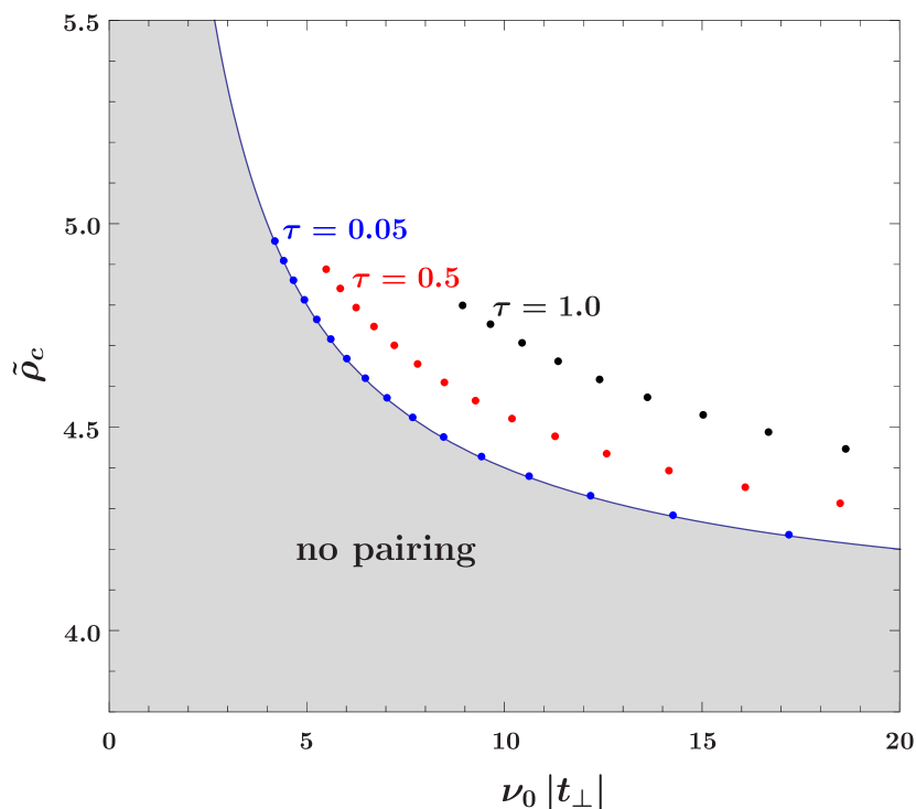
Figure 8: (Color online) Critical density $\tilde{\rho}_{c}$ for pair condensation as a function of the two-body $t$-matrix $|t_{\bot}|$ (note that $t_{\bot}<0$, so $-t_{\bot}=|t_{\bot}|$) for fixed temperatures $\tau$. The solid line depicts $\tilde{\rho}_{c}$ for vanishing temperature as given in Eq. (D10). The dots represent numerical solutions of the regularized gap equation (D9) for the indicated temperatures. The shaded area underneath the solid line represents the regime where pairing cannot occur at any temperature.

References

- (1) Y.-J. Lin, R. L. Compton, A. R.Perry, W. D. Phillips, J. V. Porto, and I. B. Spielman, Phys. Rev. Lett. 102, 130401 (2009); Y.-J. Lin, R. L. Compton, K. Jiménez-García, J. V. Porto, and I. B. Spielman, Nature 462, 628 (2009); Y.-J. Lin, R. L. Compton, K. Jiménez-García, W. D. Phillips, J. V. Porto, and I. B. Spielman, Nature Phys. 7, 531 (2011); Y.-J. Lin, K. Jiménez-García, and I. B. Spielman, Nature 471, 83 (2011); R. A. Williams, L. J. LeBlanc, K. Jiménez-García, M. C. Beeler, R. A. Perry, W. D. Phillips, and I. B. Spielman, Science 335, 314 (2011).
- (2) J. Dalibard, F. Gerbier, G. Juzeliũnas, and P. Öhberg, Rev. Mod. Phys. 83, 1523 (2011).
- (3) T. D. Stanescu, B. Anderson, and V. Galitski, Phys. Rev. A 78, 023616 (2008).
- (4) C. Wang, C. Gao, C.-M. Jian, and H. Zhai, Phys. Rev. Lett. 105, 160403 (2010); C. Wu, I. Mondragon-Shem, and X. Zhou, Chin. Phys. Lett. 28, 097102 (2011); H. Zhai, Int. J. Mod. Phys. B 26, 1230001 (2012); W. Zheng, Z.-Q. Yu, X. Cui, and H. Zhai, arXiv:1212.6832 [cond-mat.quant-gas].
- (5) S. Gopalakrishnan, A. Lamacraft, and P. M. Goldbart, Phys. Rev. A 84, 061604(R) (2011).
- (6) T.-L. Ho and S. Zhang, Phys. Rev. Lett. 107, 150403 (2011).
- (7) T. Ozawa and G. Baym, Phys. Rev. A 84, 043622 (2011); Phys. Rev. Lett. 109, 025301 (2012); Phys. Rev. A 85, 013612 (2012); Phys. Rev. Lett. 110, 085304 (2013).
- (8) R. Barnett, S. Powell, T. Graß, M. Lewenstein, and S. Das Sarma, Phys. Rev. A 85, 023615 (2012).
- (9) T. A. Sedrakyan, A. Kamenev, and L. I. Glazman, Phys. Rev. A 86, 063639 (2012).
- (10) H. Hu and X.-J. Liu, Phys. Rev. A 85, 013619 (2012).
- (11) X. Cui and Q. Zhou, Phys. Rev. A 87, 031604(R) (2013); Q. Zhou and X. Cui, Phys. Rev. Lett. 110, 140407 (2013).
- (12) R. Liao, Z.-G. Huang, X.-M. Lin, and W.-M. Liu, Phys. Rev. A 87, 043605 (2013); W. Han, S. Zhang, and W.-M. Liu, arXiv:1211.2097 [cond-mat.quant-gas].
- (13) Y. Li, L. P. Pitaevskii, and S. Stringari, Phys. Rev. Lett. 108, 225301 (2012); Y. Li, G. I. Martone, L. P. Pitaevskii, and S. Stringari, Phys. Rev. Lett. 110, 235302 (2013).
- (14) X. Zhou, Y. Li, Z. Cai, and C. Wu, arXiv:1301.5403 [cond-mat.quant-gas] [J. Phys. B (to be published)].
- (15) Z. -Q. Yu, Phys. Rev. A. 87, 051606(R) (2013).
- (16) E. I. Rashba, Fiz. Tverd. Tela (Leningrad) 2, 1224 (1960).
- (17) A. Paramekanti, L. Balents, and M. P. A. Fisher, Phys. Rev. B 66, 054526 (2002).
- (18) S. Sachdev, Nature 418, 739 (2002).
- (19) V. I. Yukalov, Teor. Mat. Fiz. 37, 390 (1978) [Theoret. and Math. Phys. 37, 1093 (1978)].
- (20) S. A. Brazovskii, Zh. Eksp. Teor. Fiz. 68, 175 (1975) [Sov. Phys. JETP 41, 85 (1975)].
- (21) P. C. Hohenberg and J. B. Swift, Phys. Rev. E 52, 1828 (1995).
- (22) Y. Shiwa, J. Stat. Phys. 124, 1207 (2006).
- (23) P. Kopietz, L. Bartosch, and F. Schütz, Introduction to the Functional Renormalization Group, (Springer, Berlin, 2010).
- (24) P. Kopietz and T. Busche, Phys. Rev. B 64, 155101 (2001).
- (25) A. Rückriegel, A. Kreisel, and P. Kopietz, Phys. Rev. B 85, 054422 (2012).
- (26) I. M. Lifshitz, Zh. Eksp. Teor. Fiz. 38, 1569 (1960) [Sov. Phys. JETP 11, 1130 (1960)].
- (27) See, for example, T. Moriya, Spin Fluctuations in Itinerant Electron Magnetism, (Springer, Berlin, 1985).
- (28) W. Metzner, M. Salmhofer, C. Honerkamp, V. Meden, and K. Schönhammer, Rev. Mod. Phys. 84, 299 (2012).