Quantum to Classical Transition of Inflationary Perturbations
- Continuous Spontaneous Localization as a Possible Mechanism -

Abstract

The inflationary paradigm provides a mechanism to generate the primordial perturbations needed to explain the observed large scale structures in the universe. Inflation traces back all the inhomogeneities to quantum fluctuations although the structures look classical today. Squeezing of primordial quantum fluctuations along with the mechanism of decoherence accounts for many aspects of this quantum to classical transition, although it remains a matter of debate as to whether this is sufficient to explain the issue of realization of a single outcome (i.e. the issue of macro-objectification) from a quantum ensemble given that the universe is a closed system. A similar question of emergence of classical behavior of macroscopic objects exists also for laboratory systems and apart from decoherence there have been attempts to resolve this issue through Continuous Spontaneous Localization (CSL), which is a stochastic nonlinear modification of the non-relativistic Schrödinger equation. Recently, Martin et al. have investigated whether a CSL-like mechanism with a constant strength parameter, when the Mukhanov-Sasaki variable is taken as the “collapse-operator”, can explain how the primordial quantum perturbations generated during inflation become classical. Within the scope of their assumptions they essentially come to a negative conclusion. In the present work, we generalize their analysis by allowing the CSL strength parameter to depend on physical scales so as to capture the CSL amplification mechanism. We show that such a generalization provides a mechanism for macro-objectification (i.e. classicalization) of the inflationary quantum perturbations, while also preserving scale invariance of the power spectrum and phase coherence of super-horizon perturbation modes in a particular class of these models.

I Introduction

Inflation Guth:1980zm ; Linde:1981mu is an early phase of accelerated expansion which apart from solving shortcomings of the Big Bang cosmology, such as the horizon and flatness problems, also provides a natural mechanism to seed the primordial inhomogeneities which grow into the structures we observe today Mukhanov:1990me ; Baumann:2009ds . The basic predictions of inflationary paradigm such as approximate scale-invariance and Gaussianity of primordial power spectrum are supported very well by Cosmic Microwave Background (CMB) Hinshaw:2012fq ; Ade:2013uln and large scale structure data Abazajian:2008wr . Inflationary cosmology has also been used as a testing ground of many alternative theories like Lorentz violating theories Loretnzviolate , modified gravity theories Modified and more recently some modified quantum theories Sudarsky1 ; Sudarsky2 ; Sudarsky3 ; Sudarsky4 ; Sudarsky5 in order to constrain them.

The mechanism of generating the primordial inhomogeneities by inflation is essentially amplifying the quantum fluctuations of a scalar field. But the large scale structures like galaxies do behave like classical objects. This then leads us to the problem of understanding quantum to classical transition in the cosmological context which can be thought as a more serious form of the so-called ‘quantum measurement problem’. The key conceptual issue of quantum mechanics has been the appearance of deterministic outcomes in a measurement process one performs over a quantum system prepared in a superposed state. The quantum theory, if endowed with the Copenhagen interpretation, suggests that a quantum state remains in a superposed state as long as no observer does a measurement on it. As soon as the observer performs a measurement on the quantum state, the interaction of the state with the classical measuring apparatus causes the quantum state to ‘collapse’ into one of the eigenstates of the observable being measured by the apparatus. This age-old heuristic description has since been drastically refined with the understanding of the phenomenon of decoherence where the classical apparatus is coupled to an environment consisting of a very large number of degrees of freedom, which one is not concerned about in a measurement process Zurek:1981xq ; Zurek:1982ii ; Joos:1984uk . However, it has been argued that the formalism of decoherence by itself does not solve the problem of a single outcome Adler:2001us ; Schlosshauer:2003zy . For completion, decoherence must be supplemented with the formalism of many-worlds Everett:1957hd , thus making it debatable and possibly not acceptable to a section of the community. Secondly this scheme relies heavily on a distinction between the ‘environment’ and the ‘system’. Therefore, this scheme does not naturally extend to closed systems such as the early universe. There have been other attempts dealing with these kind of issues such as Bohmian mechanics Bohm:1951xw ; Bohm:1951xx but these do not by themselves predict a testable feature of the model which can be verified or refuted.

As has been mentioned earlier, the problem of quantum measurement associated with the interpretation of quantum theory manifests itself also in the context of appearance of large scale structures such as galaxies and clusters in the universe. So the issue which becomes pertinent is: at what stage these fluctuations lose their quantum features to attain classical characteristics during the process of evolution? And what is the mechanism which brings about this quantum-to-classical transition? What we observe through CMBR is in a sense a measurement of the field variable Kiefer:2008ku ; Kiefer:2006je ; Kiefer:1998qe and the definiteness in the result of the measurement indicates that the field eigenstates get selected as the privileged basis.

Decoherence has been suggested as a plausible framework to deal with these open problems Kiefer:2008ku ; Kiefer:2006je ; Kiefer:1998qe ; Polarski:1995jg . It turns out to be useful to work with a gauge invariant quantity known as the Mukhanov-Sasaki variable to study the evolution of the fluctuations. It is interesting to note that during the course of evolution the probability distribution of the Mukhanov-Sasaki variable gets highly squeezed Kiefer:2008ku ; Kiefer:2006je ; Kiefer:1998qe ; Polarski:1995jg ; Martin:2012pe in the phase space along momentum. It is shown that in this high squeezing limit the quantum expectations can be well mimicked by statistical average over a classical stochastic field Kiefer:1998jk . In this sense, one can study the evolution of these fluctuations through classical equations and take the fluctuations as classical for all practical purposes. This is clearly one facet of explaining the classical nature of the structures in the universe. Moreover decoherence selects field eigenstates as the pointer basis and eventually one arrives at a diagonal density matrix which is a characteristic of classical systems.

However, one can still ask the question analogous to the issue of ‘macro-objectification’ in quantum mechanics i.e. how does a particular realization of the system get selected. Furthermore, from the CMBR spectra we learn that selection of field eigenbasis as pointer basis and the collapse of the field in one of the field eigenbasis occurs at least as early as the epoch of recombination since the radiation essentially free-streams through the universe after recombination. CMBR encodes the signature of the initial density perturbations which started to grow after recombination. Thus the CMB map, in a sense, carries information about a measurement of the field variable, which took place at least as early as recombination when there were no ‘conscious observers’ to cause collapse. Therefore, these interpretational issues, as we see, become very significant when applied to the early universe. Classicalization by decoherence does not naturally extend to closed systems such as the early universe. As there were neither natural degrees of freedom to act as an ‘environment’ nor observers who update their knowledge about the system, the schemes such as decoherence or state depicting the knowledge of an observer might seem inadequate to deal with the evolution of the universe.

One possible way to approach interpretational issues such as the quantum measurement problem is to consider dynamically induced collapse of the wave-function. For instance, collapse may be induced by gravity, or by modifications of quantum theory. Such modifications will have implications for inflationary dynamics, and their role in generating classical density perturbations has been analyzed extensively by Sudarsky and collaborators Sudarsky1 ; Sudarsky2 ; Sudarsky3 ; Sudarsky4 ; Sudarsky5 .

Continuous Spontaneous Localization (CSL) is a phenomenological model which tries to address these interpretational issues related to the quantum theory Bassi:2003gd ; Bassi:2012bg . In this scheme one makes non-linear, non-hermitean stochastic modifications to the evolution equations otherwise governed by the hermitean Hamiltonian. The defining feature of these corrections is that they drive the state to one of the eigenstates of position (in the position driven models) which is a description of localization. The quantum measurement process is understood in this framework with the understanding that any measurement is essentially a position measurement Bassi:2003gd ; Bassi:2012bg . One important aspect of the modifications is that they are very tiny for microscopic systems resulting in the longevity of the superposed states, while they grow substantially large for macroscopic systems (the so-called amplification mechanism) causing a quick and effective position localization of macroscopic objects. Being a phenomenological modification of quantum theory, its parameters are constrained through studying the effects of such models on laboratory as well as cosmological situations Bassi:2003vf ; Adler:2004un ; Adler:2004rf ; Pearle:2007rw ; Pearle:2010uu ; Lochan:2012di . For a detailed introduction of this scheme the reader is referred to Bassi:2003gd ; Bassi:2012bg .

Although this scheme is phenomenological and only developed for non-relativistic systems, motivated by the features of this scheme Martin et al. Martin:2012pe recently attempted a generalization of adding stochastic modification to quantum theory to study the evolution of the very early universe. As a relativistic generalization of CSL has not yet been successfully achieved Pearle:2005rc ; Pearle:1976ka ; Ghirardi:1985mt ; Pearle:1988uh ; Ghirardi:1989cn ; Bassi:2003gd ; Weinberg:2011jg , in this case they introduce a CSL-like correction in the functional Schrödinger equation for evolution of mode functions. They show that this analysis is precisely equivalent to consideration of a harmonic oscillator with time dependent frequency in the original CSL model. The motivation is to obtain classicalization for super-horizon modes in a single realization of the universe. However, for simplicity they primarily consider a model with a constant collapse strength parameter $\gamma$ in Mukhanov-Sasaki variable driven collapse mechanism which lacks the mechanism of scale-dependent amplification as we will discuss below. The amplification mechanism in the non-relativistic collapse model (which assumes $\gamma$ to be mass-dependent) causes the non-linear stochastic corrections to become dominant for macro-objects causing an effective and efficient collapse. The outcome of their analysis with constant $\gamma$ model is that one does not obtain an efficient collapse of the field variable. Moreover, they show that such modifications leave undesirable imprints on the power spectrum by making it scale-dependent. The requirement that these modes must reside outside the current cosmological horizon, motivated by the fact that the power spectrum we observe is scale invariant, constrains the parameter $\gamma$ to exponentially suppressed values. Although the time available for collapse process is sufficient with the constrained parameter, the suppressed value of the CSL correction parameter $\gamma$ makes the collapse inefficient as the width of localization is inversely related to $\gamma$.

This scheme adopted by Martin et al. although certainly being a preliminary and interesting step towards obtaining the guiding principles for a field theoretic generalization of CSL, has some limitations, in our opinion. The first and obvious one, as pointed out by them, is the lack of an amplification mechanism dependent on the relevant length scales. As discussed before, the amplification mechanism is the source of different behavior of macro or micro-objects. One in general, does not expect an efficient collapse in the absence of this mechanism. Had the collapse process without the amplification been still effective, one would be lead to the conclusion that modes with smallest length scales are as effectively classicalized as modes with large length scales rendering any quantum phenomenon for any length scale. Therefore, it will be a natural demand to ask for a CSL generalization which calls for a distinction between micro and macro modes.

Secondly, one learns that such a scheme is capable of distorting the scale invariant power spectrum for the modes where the CSL correction is dominating over the standard quantum evolution. Furthermore, in normal CSL scenario one expects an efficient collapse to occur in the above mentioned regime. Thus when one suggests that the modes which distort the power spectrum lie outside the current horizon, one is lead to the argument that the modes physically relevant to us and within the horizon today are the ones least affected by CSL modifications. However these are the modes which one sought to be classicalized by the CSL mechanism, i.e. dominated by the CSL modifications. Thus one should ask for a mechanism which not only captures the amplification mechanism but also respects the observed scale invariant power spectrum.

Our scheme in this paper will be to constrain the class of CSL type modifications in the spirit of Martin et al. by consideration of the above mentioned criteria. We will see that the inefficiency of the constant $\gamma$ models is manifested at the level of Wigner function itself, even before constraining $\gamma$ to a insignificantly small value when confronted with observations. As argued before, to take into account this discrepancy we will modify the CSL parameter $\gamma$ to carry information about different modes. We show that any time invariant model is as inefficient as a constant $\gamma$ case for MS variable driven collapse. Therefore, we introduce scale dependence in this parameter. In such a case, we observe that unless the scale dependence of $\gamma$ is sufficiently strong there is no localization in the field variable. If the parameter lies in a certain allowed range then we obtain desired effective collapse in field eigenbasis in the superhorizon limit. We further constrain the model by considering the scale-invariance of the power spectrum. We show that a particular class of scale dependent models seems capable of meeting these requirements. Further, the appearance of acoustic peaks in the CMBR map is a signature of phase coherence of primordial perturbations which appears very naturally in standard inflationary scenarios Dodelson:2003ip ; Albrecht:1995bg . In the class of collapse models which respect the scale-invariance of power spectrum we argue that the phase coherence is not destroyed.

The paper is organized as follows. We briefly introduce the inflationary perturbations in the standard framework in the Heisenberg as well as Schrödinger picture in section II. Here we also discuss the concept of squeezing and the understanding of classicalization through it. In section III, we briefly review the CSL model and discuss the models of constant $\gamma$ (as well as $\gamma(k)$) in inflationary context to study its effects on squeezing and power spectrum. Section IV describes the introduction of amplification mechanism in the form of scale dependent $\gamma$ model. We discuss its effect on power spectrum and constrain the models which respect the scale invariance of the power spectrum. In section V, we discuss the issue of phase coherence in the light of the CSL type modification. We then summarize our main results in section VI and conclude.

II Inflationary Perturbations in Heisenberg and Schrödinger picture and squeezed states

In general, the perturbations generated during inflation are studied in the Heisenberg picture Mukhanov:1990me . We, on the other hand, need to study the evolution of these primordial perturbations in the Schrödinger picture: this will help us incorporate the CSL mechanism within the arena of inflation. These two representations of quantum fluctuations are equivalent and provide the same physical implications for the derived quantities. As the Schrödinger picture of evolution of primordial fluctuations is less studied in the literature, we will recall here the evolution of mode functions in a generic inflationary scenario (especially the squeezing of the modes) in both the pictures; this will help us relate the more conventional Heisenberg picture analysis of the inflationary modes with that of the Schrödinger picture.

II.1 Heisenberg Picture

We first provide a brief account of the inflationary perturbations and the squeezing of the modes in the Heisenberg picture, following Polarski:1995jg . Considering only the scalar fluctuations of a perturbed FRW metric in conformal time $\tau$

$$ds^{2}=a^{2}(\tau)\left[-(1-2A)d\tau^{2}+2(\partial_{i}B)dx^{i}d\tau+\left\{(1-2\psi)\delta_{ij}+2\partial_{i}\partial_{j}E\right\}dx^{i}dx^{j}\right],$$ (1)

one can combine the fluctuations of the inflaton field $\varphi(\tau,\mathbf{x})\equiv\varphi_{0}(\tau)+\delta\varphi(\tau,\mathbf{x})$ and the scalar degrees of freedom of the perturbed FRW metric to construct gauge-invariant quantities as

$$\Phi_{B}(\tau,\mathbf{x}) = A+\frac{1}{a}\left[a(B-E^{\prime})\right]^{\prime},$$ (2)

$$\delta\varphi^{\rm gi}(\tau,\mathbf{x}) = \delta\varphi+\varphi_{0}^{\prime}(B-E^{\prime}),$$ (3)

where $x^{\prime}\equiv{dx}/{d\tau}$ and $\Phi_{B}$ is known as the Bardeen potential. These two gauge-invariant quantities, $\Phi_{B}$ and $\delta\varphi^{\rm gi}$, are related to each other by perturbed Einstein equations. A combination of these two gauge-invariant quantities, known as the Mukhanov-Sasaki (MS) variable

$$\zeta(\tau,\mathbf{x})=a\left[\delta\varphi^{\rm gi}+\varphi_{0}^{\prime}\frac{\Phi_{B}}{\mathcal{H}}\right],$$ (4)

where $\mathcal{H}={a^{\prime}}/{a}$, is often studied in the context of evolution of primordial fluctuations, because in the absence of anisotropic stress in the energy-momentum tensor the MS variable is related to the comoving curvature perturbation $\mathcal{R}$:

$$\zeta(\tau,\mathbf{x})=\frac{a\varphi_{0}^{\prime}}{\mathcal{H}}\mathcal{R}(\tau,\mathbf{x}).$$ (5)

The curvature perturbation remains conserved on super-horizon scales.

By treating it as a field, the action of $\zeta(\tau,\mathbf{x})$ (expanding up to second order of perturbations) can be written as Mukhanov:1990me

$$S=\frac{1}{2}\int d^{4}x\left[(\zeta^{\prime})^{2}-\left(\nabla\zeta\right)^{2}+\frac{z^{\prime\prime}}{z}\zeta^{2}\right],$$ (6)

where $z\equiv{a\varphi_{0}^{\prime}}/{\mathcal{H}}=a\sqrt{2\epsilon}M_{\rm Pl}$, $\epsilon$ being the slow-roll parameter and $M_{\rm Pl}$ being the reduced Planck mass. This action is equivalent to the action

$$S=\frac{1}{2}\int d^{4}x\left[(\zeta^{\prime})^{2}-\left(\nabla\zeta\right)^{2}-2\frac{z^{\prime}}{z}\zeta\zeta^{\prime}+\left(\frac{z^{\prime}}{z}\right)^{2}\zeta^{2}\right]$$ (7)

up to a total derivative term Albrecht:1992kf .

In this paper we consider the slow-roll parameter $\epsilon$ to vary negligibly with time during inflation; this will correspond to ${z^{\prime\prime}}/{z}={a^{\prime\prime}}/{a}$ and ${z^{\prime}}/{z}={a^{\prime}}/{a}$. We also assume a quasi-de Sitter spacetime for studying the evolution of modes during inflation in which case one can write the scale factor as

$$a(\tau)=-\frac{1}{H\tau(1-\epsilon)},$$ (8)

where $H$ is the Hubble parameter. One then gets ${a^{\prime}}/{a}\approx-(1+\epsilon)/\tau$ up to first order in slow-roll parameter $\epsilon$. For convenience we neglect the slow-roll parameter (as $\epsilon\ll 1$ for quasi-de Sitter space) to keep the leading order term and consider ${a^{\prime}}/{a}=-1/\tau$ for all practical purposes.

Initially we will consider this action for analysis of squeezing of modes. Treating the scalar fluctuations classically, the conjugate momentum $p$ of the MS variable $\zeta(\tau,\mathbf{x})$ would be

$$p\equiv\frac{\partial\mathcal{L}(\zeta,\zeta^{\prime})}{\partial\zeta^{\prime}}=\zeta^{\prime}-\frac{a^{\prime}}{a}\zeta.$$ (9)

Decomposing the MS variable in Fourier modes:

$$\zeta(\tau,\mathbf{x})=\frac{1}{(2\pi)^{\frac{3}{2}}}\int d^{3}{\mathbf{k}}\,\zeta_{\mathbf{k}}(\tau)e^{i\mathbf{k\cdot x}},$$ (10)

with $\zeta_{-\mathbf{k}}=\zeta^{*}_{\mathbf{k}}$ as $\zeta(\tau,\mathbf{x})$ is real, the Hamiltonian of the system is given by

$$H\equiv\int d^{3}{\mathbf{x}}\,\mathcal{H}=\frac{1}{2}\int d^{3}{\mathbf{k}}\left[p_{\mathbf{k}}p^{*}_{\mathbf{k}}+k^{2}\zeta_{\mathbf{k}}\zeta^{*}_{\mathbf{k}}+\frac{a^{\prime}}{a}\left(\zeta_{\mathbf{k}}p^{*}_{\mathbf{k}}+\zeta^{*}_{\mathbf{k}}p_{\mathbf{k}}\right)\right]$$ (11)

and the modes $\zeta_{\mathbf{k}}$ satisfy the equation of motion

$$\zeta_{\mathbf{k}}^{\prime\prime}+\omega^{2}(\tau,k)\zeta_{\mathbf{k}}=0,$$ (12)

which is equivalent to an equation of motion of a harmonic oscillator with a time-dependent frequency

$$\omega^{2}(\tau,k)=k^{2}-\frac{a^{\prime\prime}}{a}.$$ (13)

Upon quantization of the classical field $\zeta(\tau,\mathbf{x})$, the Fourier transforms $\zeta_{\mathbf{k}}$ are promoted to operators as

$$\hat{\zeta}_{\mathbf{k}}=\frac{a_{\mathbf{k}}+a^{\dagger}_{-\mathbf{k}}}{\sqrt{2k}}\,,\quad\quad\hat{p}_{\mathbf{k}}=-i\sqrt{\frac{k}{2}}\left(a_{\mathbf{k}}-a^{\dagger}_{-\mathbf{k}}\right),$$ (14)

and the canonical commutation relations

$$\left[\hat{\zeta}(\tau,\mathbf{x}),\hat{p}(\tau,\mathbf{y})\right]=i\delta^{3}(\mathbf{x}-\mathbf{y})$$ (15)

provide the commutation relations in the Fourier space as

$$\left[\hat{\zeta}(\tau,\mathbf{k}),\hat{p}^{\dagger}(\tau,\mathbf{k^{\prime}})\right] = i\delta^{3}(\mathbf{k}-\mathbf{k^{\prime}}),$$

$$\left[a(\tau,\mathbf{k}),a^{\dagger}(\tau,\mathbf{k^{\prime}})\right] = \delta^{3}(\mathbf{k}-\mathbf{k^{\prime}}).$$ (16)

Hence the classical Hamiltonian given in Eqn. (11) yields the Hamiltonian operator:

$$\hat{H}=\frac{1}{2}\int d^{3}{\mathbf{k}}\left[k\left\{a_{\mathbf{k}}a^{\dagger}_{\mathbf{k}}+a^{\dagger}_{-\mathbf{k}}a_{-\mathbf{k}}\right\}-i\frac{a^{\prime}}{a}\left\{a_{\mathbf{k}}a_{-\mathbf{k}}-a^{\dagger}_{\mathbf{k}}a^{\dagger}_{-\mathbf{k}}\right\}\right].$$ (17)

For the above Hamiltonian one gets the time evolution of the creation and annihilation operators as

$$\left(\begin{array}[]{c}a^{\prime}_{\mathbf{k}}\\ a^{\dagger\prime}_{-\mathbf{k}}\end{array}\right)=\left(\begin{array}[]{ccc}-ik&&\frac{a^{\prime}}{a}\\ \frac{a^{\prime}}{a}&&ik\end{array}\right)\left(\begin{array}[]{c}a_{\mathbf{k}}\\ a^{\dagger}_{-\mathbf{k}}\end{array}\right).$$ (24)

A general solution for the above coupled equations is

$$a_{\mathbf{k}}(\tau) = u_{k}(\tau)a_{\mathbf{k}}(\tau_{0})+v_{k}(\tau)a^{\dagger}_{-\mathbf{k}}(\tau_{0}),$$

$$a^{\dagger}_{-\mathbf{k}}(\tau) = u^{*}_{k}(\tau)a^{\dagger}_{-\mathbf{k}}(\tau_{0})+v^{*}_{k}(\tau)a_{\mathbf{k}}(\tau_{0}),$$ (25)

which yields the commutation relation given in Eqn. (16) provided

$$|u_{k}(\tau)|^{2}-|v_{k}(\tau)|^{2}=1.$$ (26)

This also shows that $u_{k}$ and $v_{k}$ follow the evolution equations

$$u_{k}^{\prime} = -iku_{k}+\frac{a^{\prime}}{a}v_{k}^{*}\,,$$

$$v_{k}^{\prime} = -ikv_{k}+\frac{a^{\prime}}{a}u_{k}^{*}\,.$$ (27)

One can also write the Fourier transform $\zeta_{\mathbf{k}}$ in terms of mode functions $f_{k}(\tau)$ as

$$\hat{\zeta}_{\mathbf{k}}=f_{k}(\tau)a_{\mathbf{k}}(\tau_{0})+f^{*}_{k}(\tau)a^{\dagger}_{-\mathbf{k}}(\tau_{0}),$$ (28)

which satisfies the commutation relation given in Eqn. (15) provided that the conserved Wronskian satisfies

$$W=f_{k}f_{k}^{*\prime}-f_{k}^{*}f_{k}^{\prime}=i.$$ (29)

The mode function also satisfies the Euler-Lagrange equation given in Eqn. (12):

$$f_{k}^{\prime\prime}+\omega^{2}(\tau,k)f_{k}=0$$ (30)

and is related to $u_{k}$ and $v_{k}$ as

$$f_{k}=\frac{u_{k}+v_{k}^{*}}{\sqrt{2k}}.$$ (31)

We also note here that $f_{k}^{*}$, too, satisfies the second-order differential equation stated above and thus $f_{k}$ and $f_{k}^{*}$ are the two linearly independent solutions of the evolution equation of the mode functions. This is also evident from the Wronskian of $f_{k}$ and $f_{k}^{*}$ being non-zero. For the momentum modes we have

$$\hat{p}_{\mathbf{k}}=-i\left[g_{k}(\tau)a_{\mathbf{k}}(\tau_{0})-g^{*}_{k}(\tau)a^{\dagger}_{-\mathbf{k}}(\tau_{0})\right],$$ (32)

which is related to $u_{k}$ and $v_{k}$ as

$$g_{k}=\sqrt{\frac{k}{2}}(u_{k}-v_{k}^{*}).$$ (33)

We can study the evolution of the modes in terms of another set of variables $r_{k}$, $\theta_{k}$ and $\phi_{k}$ which are used in the so-called squeezed state formalism Albrecht:1992kf . Using the constraint given in Eqn. (26) the old variables $u_{k}$ and $v_{k}$ can be reparametrized as

$$u_{k}(\tau) = e^{-i\theta_{k}(\tau)}\cosh r_{k}(\tau),$$

$$v_{k}(\tau) = e^{i\theta_{k}(\tau)+2i\phi_{k}(\tau)}\sinh r_{k}(\tau),$$ (34)

where $r_{k}$ and $\phi_{k}$ are the squeezing parameter and squeezing angle respectively and $\theta_{k}$ is the phase. The evolution equation of these three parameters would be

$$r_{k}^{\prime} = \frac{a^{\prime}}{a}\cos 2\phi_{k},$$

$$\phi_{k}^{\prime} = -k-\frac{a^{\prime}}{a}\sin 2\phi_{k}\coth 2r_{k},$$

$$\theta_{k}^{\prime} = k+\frac{a^{\prime}}{a}\sin 2\phi_{k}\tanh r_{k}.$$ (35)

The above equations suggest that when $|r_{k}|\rightarrow\infty$ (which happens on super-horizon scales as we see later in this section) one gets $(\theta_{k}+\phi_{k})^{\prime}|_{|r_{k}|\rightarrow\infty}=0$. This shows that on super-horizon scales $\theta_{k}+\phi_{k}\rightarrow\delta_{k}$ where $\delta_{k}$ is some constant phase. As on super-horizon scales the mode function becomes (following Eqn. (31))

$$f_{k}|_{|r_{k}|\rightarrow\infty}\rightarrow e^{-i\delta_{k}}e^{r_{k}}\cos\phi_{k},$$ (36)

it shows that the phase of the modes becomes constant on super-horizon scales. Another way of showing that the phase of the mode functions freezes on super-horizon scales is by writing the mode functions as

$$f_{k}(\tau)=R_{k}(\tau)e^{-i\delta_{k}(\tau)},$$ (37)

which yields the evolution equation of the amplitude $R_{k}$ and phase $\delta_{k}$ as

$$R_{k}^{\prime\prime}+(\omega^{2}-\delta_{k}^{{}^{\prime}2})R_{k} = 0,$$

$$\delta_{k}^{\prime\prime}+2\frac{R_{k}^{\prime}}{R_{k}}\delta_{k}^{\prime} = 0.$$ (38)

The second equation shows that $\delta_{k}^{\prime}=0$ is a fixed point solution of this equation and this also shows that the amplitude $R_{k}$ follows the same evolution equation as $f_{k}$ on super-horizon scales. We will see in more detail in Sec. V, how this freezing of phases, in standard inflation, is related to the appearance of acoustic peaks in the CMBR.

Also, the solutions for the evolution equation of mode functions for a massless scalar are

$$f_{k} = \frac{1}{\sqrt{2k}}\left(1-\frac{i}{k\tau}\right)e^{-ik\tau},$$

$$g_{k} \equiv i\left(f_{k}^{\prime}-\frac{a^{\prime}}{a}f_{k}\right)=\sqrt{\frac{k}{2}}e^{-ik\tau},$$ (39)

which, after some straightforward calculations, yield

$$r_{k} = \sinh^{-1}\left(\frac{1}{2k\tau}\right),$$

$$\phi_{k} = \frac{\pi}{4}-\frac{1}{2}\tan^{-1}\left(\frac{1}{2k\tau}\right),$$

$$\theta_{k} = k\tau+\tan^{-1}\left(\frac{1}{2k\tau}\right)$$ (40)

and satisfy the set of evolution equations given in Eqn. (35). The first equation shows that for super-horizon modes when $-k\tau\rightarrow 0$ one has $|r_{k}|\rightarrow\infty$. Similarly $\phi_{k}\rightarrow\pi/2$ and $\theta_{k}\rightarrow-\pi/2$ on super-horizon scales. We will later see these parameters signify the probability distribution of the wavefunctional in the phase space characterized by the Wigner function Kiefer:2008ku ; Kiefer:2006je ; Kiefer:1998qe ; Martin:2012pe . While $r_{k}$ measures the excitation of the quantum state, $\phi_{k}$ signifies the sharing of the excitation of the state between the canonical variables Albrecht:1992kf . In the super-horizon limit we will see that in the standard inflationary scenario the wavefunctional will become squeezed in the direction of momentum conjugate to the field variable. Furthermore it can be argued that such a squeezed Wigner function characterizes a classical stochastic distribution of the field amplitude while the phase of the field variable gets fixed. In other words, the quantum expectations can be equivalently studied through averages over a classical stochastic field Kiefer:2008ku ; Kiefer:2006je ; Kiefer:1998qe ; Martin:2012pe .

II.1.1 Power spectrum

The quantum fluctuations generated during inflation lead to quite a few observational implications for the CMBR anisotropy spectrum we observe today. One such important aspect of generic inflationary scenarios is to predict a scale-invariant power spectrum of the temperature fluctuations of the CMBR. To see that we first study the power spectrum of the MS variable which is defined as the two-point correlation function of these fluctuations:

$$\langle 0|\zeta(\tau,\mathbf{x})\zeta(\tau,\mathbf{x})|0\rangle=\int\frac{dk}{k}\mathcal{P}_{\zeta}(k),$$ (41)

where

$$\mathcal{P}_{\zeta}(k)=\frac{k^{3}}{2\pi^{2}}|f_{k}|^{2}.$$ (42)

Using Eqn. (5) we see that the power spectrum of the comoving curvature perturbation $\mathcal{R}$ is related to the power spectrum of MS variable as

$$\mathcal{P}_{\mathcal{R}}(k)=\left(\frac{\mathcal{H}}{a\varphi_{0}^{\prime}}\right)^{2}\mathcal{P}_{\zeta}(k)=\frac{1}{2\epsilon a^{2}M^{2}_{\rm Pl}}\mathcal{P}_{\zeta}(k)\equiv A_{S}k^{n_{S}-1},$$ (43)

where $A_{S}$ determines the amplitude of the power for wavenumber $k$ and the scalar spectral index $n_{S}$ provides the scale-dependence of the power.

As has been mentioned before, the curvature perturbation $\mathcal{R}$ remains conserved on super-horizon scales and thus remains insensitive to the complicated cosmological evolutions after inflation like reheating. These primordial cosmological perturbations therefore can be directly measured by measuring the perturbations in the temperature $\left(\frac{\delta T}{T}\right)$ of the CMBR where these two kind of perturbations are related to each other at the surface of last-scattering as

$$\left(\frac{\delta T}{T}\right)(\mathbf{e})=\frac{1}{5}\mathcal{R}\left[\tau_{lss},-\mathbf{e}(\tau_{lss}-\tau_{0})+\mathbf{x}_{0}\right],$$ (44)

where $\mathbf{e}$ is the direction in the sky where the temperature fluctuation is measured, $\tau_{lss}$ and $\tau_{0}$ are the conformal times at surface of last scattering and today respectively and $\mathbf{x}_{0}$ is the present position from where the fluctuations are measured. Hence the power spectrum of comoving curvature perturbations is directly related to the two-point correlation function of the temperature anisotropies in the CMBR which are accurately measured by many present-day high precision observations such as WMAP Hinshaw:2012fq and PLANCK Ade:2013uln . These observations are all in agreement with a scale-invariant power spectrum with $n_{S}\approx 1$.

Analytically also we see that for the quasi-de Sitter case where $a\sim-1/\tau$ and $|f_{k}|^{2}\sim 1/k^{3}\tau^{2}$ (using Eqn. (39)) for super-horizon modes, one obtains a scale-invariant power spectrum for comoving curvature perturbations which is in accordance with these observations and signifies that each mode carries the same power during evolution.

II.2 Schrödinger Picture

Now, we will try to correlate the Schrödinger picture of evolution of modes with the Heisenberg picture discussed in the previous section following Polarski:1995jg . In the Heisenberg picture the vacuum $|0,\tau_{0}\rangle$ of the quantum state is defined at some time $\tau_{0}$ as

$$a_{\mathbf{k}}(\tau_{0})|0,\tau_{0}\rangle_{H}=0.$$ (45)

One can see from Eqn. (28) and Eqn. (32) that the vacuum is an eigenstate of the operator $\hat{\zeta}_{\mathbf{k}}+i\Omega^{-1}_{k}\hat{p}_{\mathbf{k}}$:

$$\left\{\hat{\zeta}_{\mathbf{k}}+i\Omega_{k}^{-1}(\tau)\hat{p}_{\mathbf{k}}\right\}|0,\tau_{0}\rangle_{H}=0,$$ (46)

where the time-dependent function $\Omega_{k}(\tau)$ is defined as

$$\Omega_{k}=k\frac{u_{k}^{*}-v_{k}}{u_{k}^{*}+v_{k}}\equiv\frac{g_{k}^{*}}{f_{k}^{*}}=-i\frac{f_{k}^{*^{\prime}}}{f_{k}^{*}}+i\frac{a^{\prime}}{a}.$$ (47)

On the other hand, in the Schrödinger picture the time-evolved vacuum state satisfies the equation

$$\left\{\hat{\zeta}_{\mathbf{k}}(\tau_{0})+i\Omega_{k}^{-1}(\tau)\hat{p}_{\mathbf{k}}(\tau_{0})\right\}|0,\tau\rangle_{S}=0\,,$$ (48)

and the vacuum state $|0,\tau\rangle_{S}$ corresponds to a Gaussian wave functional of the form

$$\Psi\left[\zeta_{\mathbf{k}}(\tau_{0})\zeta_{-\mathbf{k}}(\tau_{0})\right]=N_{k}(\tau)\exp\left(-\Omega_{k}\zeta_{\mathbf{k}}(\tau_{0})\zeta_{-\mathbf{k}}(\tau_{0})\right).$$ (49)

Writing $\zeta_{\mathbf{k}}(\tau)$ in real and imaginary parts as

$$\zeta_{\mathbf{k}}(\tau)=\frac{1}{\sqrt{2}}\left(\zeta_{\mathbf{k}}^{\rm R}(\tau)+i\zeta^{\rm I}_{\mathbf{k}}(\tau)\right),$$ (50)

allows us to write the real and imaginary Gaussian part of the wave functional given in Eqn. (49) as

$$\Psi_{\mathbf{k}}^{\rm R,I}\left[\tau,\zeta^{\rm R,I}_{\mathbf{k}}\right]=\sqrt{N_{k}(\tau)}\exp\left(-\frac{\Omega_{k}(\tau)}{2}\left(\zeta_{\mathbf{k}}^{\rm R,I}\right)^{2}\right),$$ (51)

where the total wave function is

$$\Psi\left[\zeta(\tau,\mathbf{x})\right]=\prod_{\mathbf{k}}\Psi_{\mathbf{k}}\left[\zeta^{\rm R}_{\mathbf{k}}(\tau),\zeta^{\rm I}_{\mathbf{k}}(\tau)\right]=\prod_{\mathbf{k}}\Psi_{\mathbf{k}}^{\rm R}\left[\zeta^{\rm R}_{\mathbf{k}}(\tau)\right]\Psi_{\mathbf{k}}^{\rm I}\left[\zeta^{\rm I}_{\mathbf{k}}(\tau)\right]$$ (52)

As each mode $\mathbf{k}$ evolves independently and so do the real and imaginary parts of their wavefunctional, for each mode $\mathbf{k}$ the real and imaginary parts of the wavefunctional $\Psi_{\mathbf{k}}^{\rm R,I}$ satisfy the functional Schrödinger equation:

$$i\frac{\partial\Psi_{\mathbf{k}}^{\rm R,I}}{\partial\tau}=\hat{\mathcal{H}}^{\rm R,I}_{\mathbf{k}}\Psi^{\rm R,I}_{\mathbf{k}},$$ (53)

where the Hamiltonian $\hat{\mathcal{H}}_{\mathbf{k}}\equiv\hat{\mathcal{H}}^{\rm R}_{\mathbf{k}}+\hat{\mathcal{H}}^{\rm I}_{\mathbf{k}}$ is as given in Eqn. (11) but with operator $\hat{p}$ and $\hat{\zeta}$.

II.2.1 Schrödinger picture analysis with the equivalent action (without the boundary term) and the power spectrum

We stated before that the two actions given in Eqn. (6) and Eqn. (7) are equivalent and analyzed the properties of squeezing parameters considering the action given in Eqn. (7). The other action given in Eqn. (6) has the advantage that the Hamiltonian of this action turns out to be analogous to that for a harmonic oscillator:

$$H\equiv\int d^{3}{\mathbf{x}}\,\mathcal{H}=\frac{1}{2}\int d^{3}{\mathbf{k}}\left[p_{\mathbf{k}}p^{*}_{\mathbf{k}}+\left(k^{2}-\frac{z^{\prime\prime}}{z}\right)\zeta_{\mathbf{k}}\zeta^{*}_{\mathbf{k}}\right]$$ (54)

where the conjugate momentum in Fourier space is

$$p_{\mathbf{k}}=\frac{\partial{\mathcal{L}}}{\partial\zeta_{\mathbf{k}}^{\prime}}=\zeta^{*\prime}_{\mathbf{k}}.$$ (55)

This is very convenient for our analysis of the CSL mechanism in inflation as the treatment of the harmonic oscillator of quantum mechanics within CSL mechanism has been studied in the literature Martin:2012pe . Hence writing the Hamiltonian for the MS variable modes in the form of a harmonic oscillator helps us incorporate CSL-like terms in its functional Schrödinger equation.

If we consider the following action for the functional Schrödinger equation given in Eqn. (53)

$$\hat{\mathcal{H}}^{\rm R,I}_{\mathbf{k}}=-\frac{1}{2}\frac{\partial^{2}}{\partial\left(\zeta^{\rm R,I}_{\mathbf{k}}\right)^{2}}+\frac{1}{2}\omega^{2}\left(\zeta^{\rm R,I}_{\mathbf{k}}\right)^{2},$$ (56)

where $\omega^{2}$ is given in Eqn. (13), then one has to determine the corresponding Gaussian functional $\Psi$ which would satisfy Eqn. (53). Putting the real and imaginary part of the wave functional into the functional Schrödinger equation we get

$$i\frac{N_{k}^{\prime}}{N_{k}}=\Omega_{k},\quad\quad\Omega_{k}^{\prime}=-i\Omega_{k}^{2}+i\omega^{2}(\tau,k).$$ (57)

However, with this Hamiltonian one obtains $g_{k}^{*}=-if_{k}^{*^{\prime}}$ which yields

$$\Omega_{k}=k\frac{u_{k}^{*}-v_{k}}{u_{k}^{*}+v_{k}}\equiv\frac{g_{k}^{*}}{f_{k}^{*}}=-i\frac{f_{k}^{*^{\prime}}}{f_{k}^{*}}.$$ (58)

Clearly, putting this form of $\Omega_{k}$ in its evolution equation given in Eqn. (57) yields the same equation of motion of $f_{k}$ as given in Eqn. (30).

Now we can obtain the power spectrum in the Schrödinger picture following the steps in Martin:2012pe . Knowing $\Omega_{k}$ one can obtain the normalization of the wave functional as

$$|N_{k}|=\left(\frac{\rm{Re}\,\Omega_{k}}{\pi}\right)^{\frac{1}{2}}.$$ (59)

The two point correlation function of the Mukhanov-Sasaki variable is defined as

$$\langle\Psi|\zeta(\tau,\mathbf{x})\zeta(\tau,\mathbf{x})|\Psi\rangle=\int\prod_{\mathbf{k}}d\zeta^{\rm R}_{\mathbf{k}}d\zeta^{\rm I}_{\mathbf{k}}\,\Psi^{*}_{\mathbf{k}}(\zeta^{\rm R}_{\mathbf{k}},\zeta^{\rm I}_{\mathbf{k}})\,\zeta(\tau,\mathbf{x})\zeta(\tau,\mathbf{x})\,\Psi_{\mathbf{k}}(\zeta^{\rm R}_{\mathbf{k}},\zeta^{\rm I}_{\mathbf{k}}),$$ (60)

which yields Martin:2012pe

$$\langle\Psi|\zeta(\tau,\mathbf{x})\zeta(\tau,\mathbf{x})|\Psi\rangle=\frac{1}{(2\pi)^{3}}\int d{\mathbf{k}}\frac{1}{2{\rm Re}\,\Omega_{k}}.$$ (61)

The real part of $\Omega_{k}$ can be easily obtained from Eqn. (47) which turns out to be

$${\rm Re}\,\Omega_{k}=\frac{1}{2|f_{k}|^{2}},$$ (62)

using the Wronskian condition $W=i$. This gives the two-point correlation function of Mukhanov-Sasaki variable as

$$\langle\Psi|\zeta(\tau,\mathbf{x})\zeta(\tau,\mathbf{x})|\Psi\rangle=\frac{1}{(2\pi)^{3}}\int d{\mathbf{k}}\,|f_{k}|^{2},$$ (63)

which yields the power spectrum of the Mukhanov-Sasaki variable following Eqn. (41) as

$$\mathcal{P}_{\zeta}(k)=\frac{k^{3}}{2\pi^{2}}|f_{k}|^{2},$$ (64)

which is the same as obtained earlier in Heisenberg picture. In the Schrödinger picture as the wavefunctional is related to the parameter $\Omega_{k}$ it would be convenient to define the power-spectrum in terms of this parameter and thus writing $|f_{k}|^{2}=1/2{\rm Re}\,\Omega_{k}$ the power spectrum of the comoving curvature perturbations can be written as

$$\mathcal{P}_{\mathcal{R}}(k)=\frac{k^{3}}{8\pi^{2}\epsilon M^{2}_{\rm Pl}}\frac{1}{a^{2}{\rm Re}\,\Omega_{k}}.$$ (65)

Thus in order to determine the nature of power spectrum of comoving curvature perturbations we need to know the behavior of $a^{2}{\rm Re}\,\Omega_{k}$ in the super Hubble limit.

II.3 Squeezed states and classicality through Wigner function

We have earlier seen that on super-horizon scales the squeezing parameter $|r_{k}|\rightarrow\infty$ and now we will determine the correlation between this asymptotic limit of squeezing parameter $r_{k}$ and the classical nature of mode functions on super-horizon scales. In general, to analyze the nature (quantum or classical) of mode functions on super-horizon scales one determines the nature of the Wigner function. In particular, a Wigner function recognizes the correlation between position (in this case the field amplitude) and momentum (canonical to the field in this case) and for a Gaussian wavefunction it has positive values everywhere. A positive definite Wigner function can be interpreted as a classical probability distribution of a quantum state under consideration in the phase space. In quantum theory the Wigner function is defined by

$${\mathcal{W}}\left(\zeta^{\rm R}_{\mathbf{k}},\zeta^{\rm I}_{\mathbf{k}},p^{\rm R}_{\mathbf{k}},p^{\rm I}_{\mathbf{k}}\right)=\frac{1}{(2\pi)^{2}}\int dxdy\Psi^{*}\left(\zeta^{\rm R}_{\mathbf{k}}-\frac{x}{2},\zeta^{\rm I}_{\mathbf{k}}-\frac{y}{2}\right)e^{-ip^{\rm R}_{\mathbf{k}}x-ip^{\rm I}_{\mathbf{k}}y}\Psi\left(\zeta^{\rm R}_{\mathbf{k}}+\frac{x}{2},\zeta^{\rm I}_{\mathbf{k}}+\frac{y}{2}\right),$$ (66)

which then yields

$${\mathcal{W}}\left(\zeta^{\rm R}_{\mathbf{k}},\zeta^{\rm I}_{\mathbf{k}},p^{\rm R}_{\mathbf{k}},p^{\rm I}_{\mathbf{k}}\right) = \frac{\Psi\Psi^{*}}{\pi{\rm Re}\,\Omega_{k}}\exp\left[-\frac{\left(p^{\rm R}_{\mathbf{k}}+{\rm Im}\,\Omega_{k}\zeta^{\rm R}_{\mathbf{k}}\right)^{2}}{{\rm Re}\,\Omega_{k}}\right]\exp\left[-\frac{\left(p^{\rm I}_{\mathbf{k}}+{\rm Im}\,\Omega_{k}\zeta^{\rm I}_{\mathbf{k}}\right)^{2}}{{\rm Re}\,\Omega_{k}}\right]$$ (67)

$$= \frac{1}{\pi^{2}}e^{-{\rm Re}\,\Omega_{k}\left(\zeta^{\rm R^{2}}_{\mathbf{k}}+\zeta^{\rm I^{2}}_{\mathbf{k}}\right)}e^{-\frac{\left(p^{\rm R}_{\mathbf{k}}+{\rm Im}\,\Omega_{k}\zeta^{\rm R}_{\mathbf{k}}\right)^{2}}{{\rm Re}\,\Omega_{k}}}e^{-\frac{\left(p^{\rm I}_{\mathbf{k}}+{\rm Im}\,\Omega_{k}\zeta^{\rm I}_{\mathbf{k}}\right)^{2}}{{\rm Re}\,\Omega_{k}}}.$$ (68)

This shows that the Wigner function is a product of four Gaussians with the first two Gaussians having a standard deviation of $\sqrt{2/{\rm Re}\,\Omega_{k}}$ and zero mean while the last two Gaussians with a standard deviation of $\sqrt{{\rm Re}\,\Omega_{k}/2}$ and mean of ${\rm Im}\,\Omega_{k}\zeta^{\rm R}_{\mathbf{k}}$ and ${\rm Im}\,\Omega_{k}\zeta^{\rm I}_{\mathbf{k}}$ respectively. To determine the nature of the Wigner function for super-horizon modes we note that

$${\rm Re}\,\Omega_{k} = \frac{k}{\cosh(2r_{k})+\cos(2\phi_{k})\sinh(2r_{k})},$$

$${\rm Im}\,\Omega_{k} = -\frac{k\sin(2\phi_{k})\sinh(2r_{k})}{\cosh(2r_{k})+\cos(2\phi_{k})\sinh(2r_{k})}.$$ (69)

Hence on super-horizon scales when $|r_{k}|\rightarrow\infty$ one gets ${\rm Re}\,\Omega_{k}\rightarrow 0$. We also see from Eqn. (40) that $\phi_{k}\rightarrow\pi/2$ as $-k\tau\rightarrow 0$ on super-horizon scales. Thus ${\rm Im}\,\Omega_{k}\rightarrow 0$ on super-horizon scales. In this strong squeezing limit the last two Gaussians in the Wigner function would become delta functions to yield

$${\mathcal{W}}\left(\zeta^{\rm R}_{\mathbf{k}},\zeta^{\rm I}_{\mathbf{k}},p^{\rm R}_{\mathbf{k}},p^{\rm I}_{\mathbf{k}}\right)\rightarrow\frac{{\rm Re}\,\Omega_{k}}{\pi}e^{-{\rm Re}\,\Omega_{k}\left(\zeta^{\rm R^{2}}_{\mathbf{k}}+\zeta^{\rm I^{2}}_{\mathbf{k}}\right)}\delta\left(p^{\rm R}_{\mathbf{k}}\right)\delta\left(p^{\rm I}_{\mathbf{k}}\right).$$ (70)

This indicates that the Wigner function will be highly squeezed in the direction of $p_{\mathbf{k}}$ resulting in a cigar-like shape which has been shown in Fig. 1.

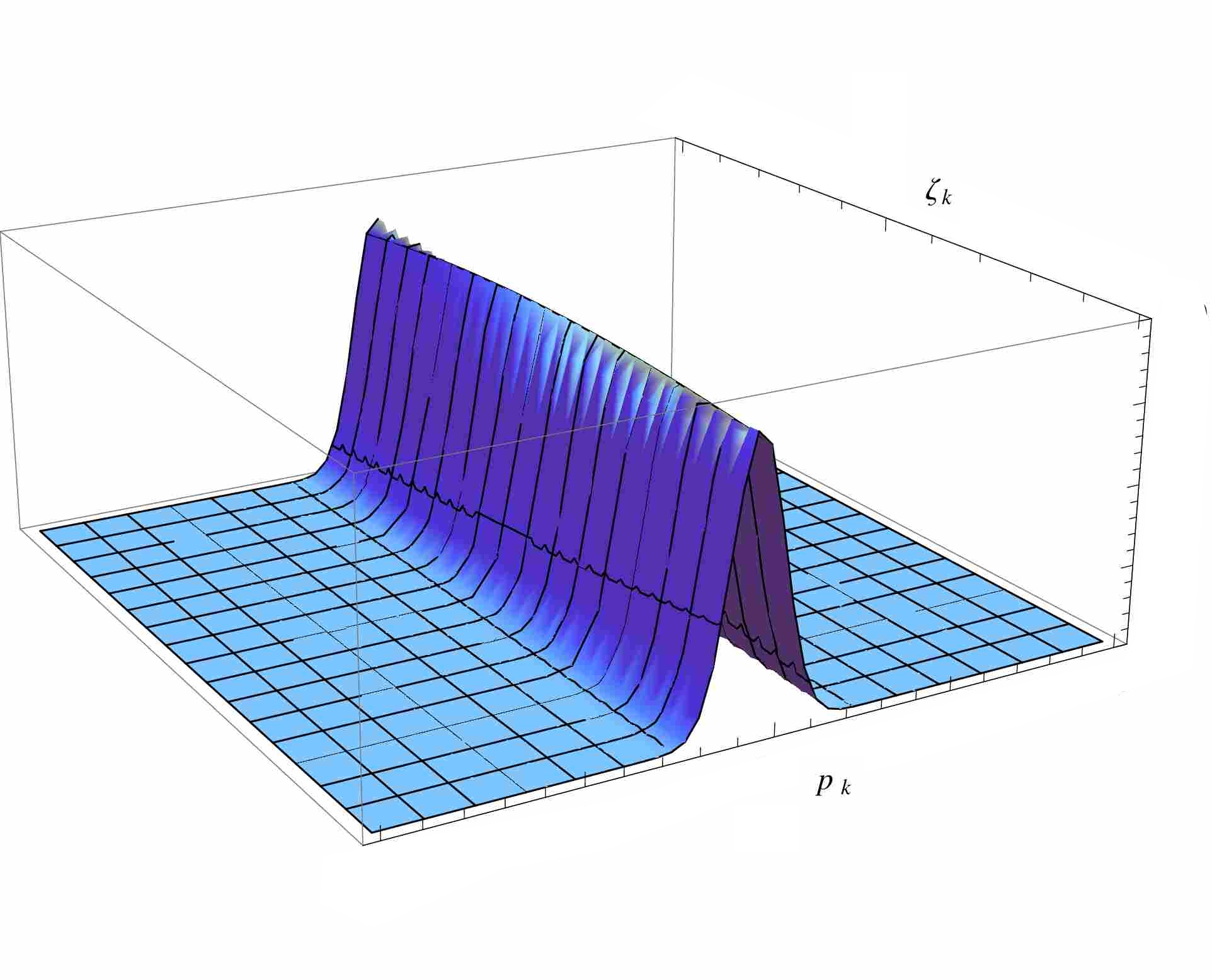
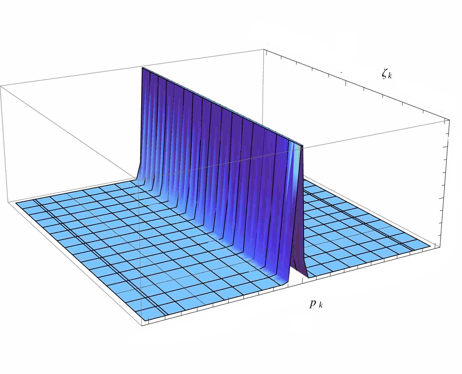
Figure 1: Plot of Wigner function for $r_{k}=2.3$ and $r_{k}=3.5$ showing high squeezing of a particular mode in the direction of momentum canonical to field variable

This highly squeezed state successfully describes how the operator expectations can be studied by considering averages over a classical stochastic field Kiefer:2008ku ; Kiefer:2006je ; Kiefer:1998qe ; Martin:2012pe . However this description presumably excludes the issue of localization of the initial perturbations in the field variable as has been observed by several CMBR experiments. For more discussions on this refer to Martin:2012pe . Later we will show the evolution of the Wigner function with CSL-like modification.

III CSL mechanism with a constant $\gamma$ and squeezing of modes during inflation

III.1 A Brief Overview of Continuous Spontaneous Localization

CSL is a dynamical mechanism aimed at answering the following conceptual issues in quantum theory: (1) Why are macroscopic objects not found in superposition of position states? (2) Why and how does the measurement process break quantum mechanical state superposition? (3) What “mass”, or, more accurately, how many nuclei, should an object possess in order to qualify as a classical measuring apparatus? (4) Why do the outcomes of a quantum measurement obey the Born probability rule?

Following the pioneering work by Pearle Pearle:1976ka and its major improvement in the framework of the Ghirardi-Rimini-Weber (GRW) model Ghirardi:1985mt , the CSL model has been proposed as an upgraded version of this model Pearle:1988uh ; Ghirardi:1989cn . CSL is designed to give a phenomenological answer to the above four questions, in the case of non-relativistic quantum mechanics. The basic physical idea behind dynamically induced wave-function collapse is that spontaneous and random wave function collapses occur all the time for all particles, whether isolated or interacting and whether they are forming a microscopic, mesoscopic or macroscopic system.

On a mathematical level, these ideas are implemented by modifying the Schrödinger equation while introducing extra terms exhibiting the following properties: (1) non-linearity so as to yield the breakdown of superposition principle at a macroscopic level, (2) stochasticity so as to be able to explain the random outcomes of a measurement process and their distribution according to the Born probability rule (stochasticity is moreover needed to avoid superluminal communication), (3) allowance for an amplification mechanism according to which the new terms have negligible effects on microscopic system dynamics but strong effects for large many-particle macroscopic systems in order to recover their classical-like behavior.

To achieve this goal, a randomly fluctuating classical field, assumed to fill all of space, couples to the quantum system number density operator to make the system collapse into its spatially localized eigenstates. The collapse process being continuous in time, the dynamics can be described in terms of a single stochastic differential equation containing features of both the standard Schrödinger evolution and wave function collapse. An outstanding open question is the origin of the random noise, or of the randomly fluctuating classical scalar field, that induces the collapse. This is where an underlying fundamental theory is needed.

The physical content of the CSL model is nicely captured by a simple model known as QMUPL (Quantum Mechanics with Universal Position Localization), described by the following non-linear Schrödinger equation Diosi89

$$d\psi_{t}=\left[-\frac{i}{\hbar}Hdt+\sqrt{\lambda}(q-\langle q\rangle_{t})dW_{t}-\frac{\lambda}{2}(q-\langle q\rangle_{t})^{2}dt\right]\psi_{t}$$ (71)

Here, $\lambda$ is a new constant of nature which determines the strength of the coupling, and is assumed proportional to the mass $m$ of the particle: $\lambda/\lambda_{0}=m/m_{0}$. This is the amplification mechanism - the strength of the non-linear modification increases with increasing mass. The mass $m$ is expressed in units of the nucleon mass $m_{0}$. If one chooses for $\lambda_{0}$ the value $10^{-2}$ m^-2 s^-1 then the collapse of the wave-function can be explained consistently with all known experimental data. $W(t)$ is the standard Wiener process [Brownian motion] which encodes the stochastic aspect. As one can see, there are two non-linear, non-unitary terms in the modified equation, one proportional to $dW(t)$, and the other proportional to $dt$. Together, the two terms relate to each other in a specific way, the latter being $(-1/2)$ times the former (since $dW^{2}=dt$). This ‘martingale’ structure of the nonlinear equation preserves norm during evolution, despite being non-unitary, and is responsible for the emergence of the Born rule.

The stochastic term prevents a wave-packet from spreading indefinitely, and causes the width of the packet to reach a finite asymptotic value. For the chosen value of the constant $\lambda_{0}$ the spread is extremely small for a macroscopic object (so that it appears to be like a particle), and very large for a microscopic system such as an electron (so that it appears to be like a wave). Thus the modified quantum dynamics is able to describe in a universal and unified manner, both the wavy nature of microscopic systems, as well as the particle nature of macroscopic objects.

As an illustration of how these effects come about, consider for simplicity a free particle $(H=p^{2}/2m)$ in the Gaussian state (the analysis can be generalized to other cases) Bassi2005 ; Bassi:2012bg

$$\psi_{t}(x)=\makebox{exp}\left[-a_{t}(x-\overline{x}_{t})^{2}+i\overline{k}_{t}x+\gamma_{t}\right].$$ (72)

By substituting this in the stochastic equation it can be proved that the spreads in position and momentum

$$\sigma_{q}(t)\equiv\frac{1}{2}\sqrt{\frac{1}{a_{t}^{\makebox{\tiny R}}}};\qquad\sigma_{p}(t)\equiv\hbar\,\sqrt{\frac{(a_{t}^{\makebox{\tiny R}})^{2}+(a_{t}^{\makebox{\tiny I}})^{2}}{a_{t}^{\makebox{\tiny R}}}},$$ (73)

do not increase indefinitely but reach asymptotic values given by

$$\sigma_{q}(\infty) = \sqrt{\frac{\hbar}{m\omega}}\simeq\left(10^{-15}\sqrt{\frac{\makebox{Kg}}{m}}\;\right)\,\makebox{m}\,,$$

$$\sigma_{p}(\infty) = \sqrt{\frac{\hbar m\omega}{2}}\simeq\left(10^{-19}\sqrt{\frac{m}{\makebox{Kg}}}\,\right)\,\frac{\makebox{Kg m}}{\makebox{s}},$$ (74)

such that: $\sigma_{q}(\infty)\,\sigma_{p}(\infty)\;=\;{\hbar}/{\sqrt{2}}$ which corresponds to almost the minimum allowed by Heisenberg’s uncertainty relations. Here, $\omega\;=\;2\,\sqrt{{\hbar\lambda_{0}}/{m_{0}}}\;\simeq\;10^{-5}\;\makebox{s${}^{-1}$}.$

The localization of the position state of macroscopic objects makes it straightforward to understand the collapse of the wave-function during a quantum measurement BassiSalvetti2007 . If a quantum system, say a two state quantum system, initially in a superposed state $(c_{+}|+\rangle+c_{-}|-\rangle)$, interacts with a measuring apparatus ${\cal A}$, the interaction causes the state to evolve to the entangled state

$$c_{+}|+\rangle{\cal A}_{1}+c_{-}|-\rangle{\cal A}_{2}$$ (75)

where ${\cal A}_{1}$ and ${\cal A}_{2}$ are respectively the pointer states of the apparatus which correspond to the microscopic system state $|+\rangle$ and $|-\rangle$. Since, as we have seen above, the stochastic dynamics prevents the apparatus (which is macroscopic) from being simultaneously in the states ${\cal A}_{1}$ and ${\cal A}_{2}$, this state ‘collapses’ into either $c_{+}|+\rangle{\cal A}_{1}$ or $c_{-}|-\rangle{\cal A}_{2}$. The structure of the modified equation ensures that the collapse probabilities obey the Born rule, and the chosen value of the constant $\lambda_{0}$ ensures that the collapse takes place sufficiently quickly. It can be proved from Eqn. (71) that the initial state Eqn. (75) evolves, at late times, to

$$\psi_{t}=\frac{|+\rangle\otimes\phi_{+}+\epsilon_{t}|-\rangle\otimes\phi_{-}}{\sqrt{1+\epsilon_{t}^{2}}}.$$ (76)

The evolution of the stochastic quantity $\epsilon_{t}$ is determined dynamically by the stochastic equation: it either goes to $\epsilon_{t}\ll 1$, with a probability $|c_{+}|^{2}$, or to $\epsilon_{t}\gg 1$, with a probability $|c_{-}|^{2}$. In the former case, one can say with great accuracy that the state vector has ‘collapsed’ to the definite outcome $|+\rangle\otimes\phi_{+}$ with a probability $|c_{+}|^{2}$. Similarly, in the latter case one concludes that the state vector has collapsed to $|-\rangle\otimes\phi_{-}$ with a probability $|c_{-}|^{2}$. This is how collapse during a quantum measurement is explained dynamically, and random outcomes over repeated measurements are shown to occur in accordance with the Born probability rule. The time-scale over which $\epsilon_{t}$ reaches its asymptotic value and the collapse occurs can also be computed dynamically. In the present example, for a pointer mass of 1 g, the collapse time turns out to be about $10^{-4}$ s.

The above QMUPL equation has been studied in quite some generality, and can be generalized to the multi-particle case as well, where it exhibits the all-important amplification property: the effective coupling strength parameter $\lambda_{eff}$ for the many-particle system scales as the total mass of the system, so that the localization effect is stronger for larger systems. The CSL model reproduces the above important properties [localization, dynamically induced collapse, amplification] of the QMUPL model while being able to deal with systems of indistinguishable particles. It is described by the following modified Schrödinger equation

$$d\psi_{t}=\left[-\frac{i}{\hbar}Hdt+\frac{\sqrt{\gamma}}{m_{0}}\int d\mathbf{x}(M(\mathbf{x})-\langle M(\mathbf{x})\rangle_{t})dW_{t}(\mathbf{x})-\frac{\gamma}{2m_{0}^{2}}\int d\mathbf{x}\,(M(\mathbf{x})-\langle M(\mathbf{x})\rangle_{t})^{2}dt\right]\psi_{t}\,.$$

The linear part is governed by $H$ - the standard quantum Hamiltonian of the system, and like in QMUPL, the other two terms induce the collapse of the wave function in space. The mass $m_{0}$ is a reference mass, which as before is taken equal to that of a nucleon. Analogous to $\lambda$, the parameter $\gamma$ is a mass-proportional [and hence possesses the amplification property] positive coupling constant which sets the strength of the collapse process, while $M({\bf x})$ is a smeared mass density operator:

$$M(\mathbf{x}) = \underset{j}{\sum}m_{j}N_{j}(\mathbf{x}),$$

$$N_{j}(\mathbf{x}) = \int d\mathbf{y}g(\mathbf{y-x})\psi_{j}^{\dagger}(\mathbf{y})\psi_{j}(\mathbf{y}),\qquad$$ (78)

$\psi_{j}^{\dagger}(\mathbf{y})$, $\psi_{j}(\mathbf{y})$ being, respectively, the creation and annihilation operators of a particle of type $j$ in the space point $\mathbf{y}$. The smearing function $g({\bf x})$ is taken equal to

$$g(\mathbf{x})\;=\;\frac{1}{\left(\sqrt{2\pi}r_{c}\right)^{3}}\;e^{-\mathbf{x}^{2}/2r_{C}^{2}},$$ (79)

where $r_{C}$ is the second new phenomenological constant of the model.

The proof for the dynamical collapse of the wave-function and the emergence of the Born probability rule in the CSL model can be found for instance in Section III.A.7 of Bassi:2012bg . The basic idea is that stochastic fluctuations drive to zero the variance $V\equiv\langle(A-\langle A\rangle)^{2}\rangle$ of the operator $A\equiv\int d\mathbf{x}\,M(\mathbf{x})$. As a consequence, the system is driven to one of the eigenstates of the measured observable. The norm-preserving martingale structure of the CSL equation ensures that the stochastic expectation of the projection operator is preserved: this coincides with the square of the amplitude in a given state, initially, and finally with the probability to result in that particular state, thus establishing the Born rule.

The CSL model is reviewed in some detail in Bassi:2012bg . An attractive feature of the model is that it is experimentally falsifiable with currently amenable technology, as its predictions depart from those of quantum theory in the mesoscopic regime. The model is being subjected to rigorous experimental tests which include molecular interferometry, optomechanics, and bounds on its fundamental parameters from astrophysical and cosmological observations Bassi:2012bg .

A novel feature of the model is that it predicts a very tiny violation of energy and momentum conservation, because of the presence of the stochastic process. While on the one hand this violation is too small to contradict known physics, it has also been suggested that such a violation induces anomalous Brownian motion, which may be detectable in laboratory experiments with mesoscopic systems CollettPearle03 .

It must be noted that CSL is a non-relativistic model, by construction. The collapse of the wave-function is an instantaneous process. While it is well understood that instantaneous collapse cannot be used for superluminal signaling, it is nonetheless an ‘action at a distance’ feature, which is not in accord with special relativity. A relativistic version of CSL would be highly desirable, but has not been achieved yet Bassi:2012bg and it has even been suggested that if verified, the CSL formalism might possibly hint at the need for a drastic revision of some basic concepts relating quantum mechanics and special relativity.

III.2 Application of a CSL-like Mechanism to Inflation

The first obstacle in applying the CSL mechanism in the inflationary paradigm to explain the classical transition of quantum mode fluctuations is that a relativistic Quantum Field Theory version of CSL model is yet to be developed and attempts to construct a viable relativistic field theoretic model of CSL face numerous problems including irremovable divergences Pearle:2005rc ; Pearle:1976ka ; Ghirardi:1985mt ; Pearle:1988uh ; Ghirardi:1989cn ; Bassi:2003gd ; Weinberg:2011jg . In spite of the lack of a proper quantum field theoretic version of CSL, Martin et al. in Martin:2012pe made an attempt to modify the functional Schrödinger equation of mode functions in Fourier space by adding ‘CSL-like’ stochastic terms with spontaneous localization on the $\hat{\zeta}_{\mathbf{k}}$ eigenmanifolds. The presence of stochasticity in the functional Schrödinger equation can be motivated from the fact that the non-relativistic limit of such a field theory should reproduce the known CSL stochastic evolution. In the non-relativistic CSL mechanism the stochastic evolution is ‘position-driven’ Bassi:2003gd ; Bassi:2012bg whereas in Martin:2012pe the addition of ‘CSL-like’ stochastic terms has been done in the Fourier basis to study the inflationary quantum fluctuations. Such a departure from the standard CSL formalism for the inflationary theories can be justified knowing that the presence of primordial non-Gaussianities are negligible so that different Fourier modes evolve independently. Having modified the functional Schrödinger equation in the field basis one would be lead to convolution of field modes in the Fourier space which will render the Gaussian nature of primordial fluctuations. Also, in such a modification the ‘CSL-like’ parameter $\gamma$ turns out to be of mass dimension 2 which is quite different from its non-relativistic version. In such a case, the bounds on the CSL parameter $\gamma$ coming from the inflationary scenario should, strictly speaking, are not to be compared with those coming from other quantum mechanical systems.

Here, we will also follow the same method of modifying the functional Schrödinger equation developed by Martin et al. for inflationary dynamics. We will consider the CSL evolution which is driven by the Mukhanov-Sasaki variable. It is important to note here that though Martin et al. added ‘CSL-like terms’ to the functional Schrödinger equation, they dealt with a constant CSL-like parameter $\gamma$ in MS variable driven model and in doing so the formalism lacks the aforementioned scale-dependent amplification mechanism. Also an inflationary CSL mechanism with a constant $\gamma$ term yields a localization in the conjugate momentum direction as in a generic case of inflationary scenario. Thus CSL mechanism with a constant $\gamma$ does not seem to have an advantage over the generic inflationary scenario. In this section we will discuss the inflationary CSL mechanism with constant $\gamma$ part and investigate the features of squeezing in this scenario. In the next section, we will present a CSL type modification which incorporates the amplification mechanism, and also explains the quantum to classical transition.

The modified functional Schrödinger equation with a constant CSL-like parameter $\gamma$ for Mukhanov-Sasaki variable is written as Martin:2012pe

$$d\Psi_{\mathbf{k}}^{\rm R,I}=\left[-i\hat{\mathcal{H}}_{\mathbf{k}}^{\rm R,I}d\tau+\sqrt{\gamma}\left(\hat{\zeta}_{\mathbf{k}}^{\rm R,I}-\left\langle\hat{\zeta}_{\mathbf{k}}^{\rm R,I}\right\rangle\right)dW_{\tau}-\frac{\gamma}{2}\left(\hat{\zeta}_{\mathbf{k}}^{\rm R,I}-\left\langle\hat{\zeta}_{\mathbf{k}}^{\rm R,I}\right\rangle\right)^{2}d\tau\right],$$ (80)

where the stochastic behavior due to CSL mechanism is encoded in the Wiener process $W_{\tau}$. We observe the formal similarity of this equation with the original CSL Eqn. (III.1). The most general stochastic wave-functional which satisfies this stochastic functional Schrödinger equation can be written as

$$\Psi^{\rm R,I}_{\mathbf{k}}\left(\tau,\zeta_{\mathbf{k}}^{\rm R,I}\right) = \left|\sqrt{N_{k}(\tau)}\right|\exp\left\{-\frac{{\rm Re}\,\Omega_{k}(\tau)}{2}\left[\zeta_{\mathbf{k}}^{\rm R,I}-\bar{\zeta}_{\mathbf{k}}^{\rm R,I}(\tau)\right]^{2}+i\sigma_{\mathbf{k}}^{\rm R,I}(\tau)+i\chi_{\mathbf{k}}^{\rm R,I}(\tau)\zeta_{\mathbf{k}}^{\rm R,I}\right.$$ (81)

$$\left.\quad\quad\quad\quad\quad\quad\quad-i\frac{{\rm Im}\,\Omega_{k}(\tau)}{2}\left(\zeta_{\mathbf{k}}^{\rm R,I}\right)^{2}\right\},$$

where $\bar{\zeta}_{\mathbf{k}}^{\rm R,I}$, $\sigma_{\mathbf{k}}^{\rm R,I}$ and $\chi_{\mathbf{k}}^{\rm R,I}$ are real numbers. If we put $\bar{\zeta}_{\mathbf{k}}^{\rm R,I}$, $\sigma_{\mathbf{k}}^{\rm R,I}$ and $\chi_{\mathbf{k}}^{\rm R,I}$ to be zero then the wave function matches with that given in Eqn. (51). A set of differential equations followed by the functions parameterizing the above functional Gaussian state is given in Martin:2012pe which we quote here for completeness:

$$\frac{|N_{k}|^{\prime}}{|N_{k}|} = \frac{1}{2}\frac{\left({\rm Re}\,\Omega_{k}\right)^{\prime}}{{\rm Re}\,\Omega_{k}}={\rm Im}\,\Omega_{k}+\frac{\gamma}{4{\rm Re}\,\Omega_{k}},$$

$$\left({\rm Re}\,\Omega_{k}\right)^{\prime} = 2\gamma+2\left({\rm Re}\,\Omega_{k}\right)\left({\rm Im}\,\Omega_{k}\right),$$

$$\left({\rm Im}\,\Omega_{k}\right)^{\prime} = -\left({\rm Re}\,\Omega_{k}\right)^{2}+\left({\rm Im}\,\Omega_{k}\right)^{2}+\omega^{2}\left(\tau,k\right),$$

$$\left(\bar{\zeta}_{\mathbf{k}}^{\mathrm{R,I}}\right)^{\prime} = \chi_{\mathbf{k}}^{\mathrm{R,I}}+\frac{\sqrt{\gamma}}{{\rm Re}\,\Omega_{k}}\frac{dW_{\tau}}{d\tau}-\left({\rm Im}\,\Omega_{k}\right)\bar{\zeta}_{\mathbf{k}}^{\mathrm{R,I}},$$

$$\left(\sigma_{\mathbf{k}}^{\mathrm{R,I}}\right)^{\prime} = -\frac{1}{2}{\rm Re}\,\Omega_{k}+\frac{1}{2}\left({\rm Re}\,\Omega_{k}\right)^{2}\left(\bar{\zeta}_{\mathbf{k}}^{\mathrm{R,I}}\right)^{2}-\frac{1}{2}\left(\chi_{\mathbf{k}}^{\mathrm{R,I}}\right)^{2},$$

$$\left(\chi_{\mathbf{k}}^{\mathrm{R,I}}\right)^{\prime} = -\left({\rm Re}\,\Omega_{k}\right)^{2}\bar{\zeta}_{\mathbf{k}}^{\mathrm{R,I}}+\chi_{\mathbf{k}}^{\mathrm{R,I}}\left({\rm Im}\,\Omega_{k}\right).$$ (82)

We see from the above set of equations that the evolution of $N_{k}$ and $\Omega_{k}$ does not depend upon the other parameters of the wave functional. Also we have seen before that $N_{k}$ and $\Omega_{k}$ are the two parameters required to determine the Wigner function. From the first equation of the set of equations given above we get

$$|N_{k}|=\left(\frac{\rm{Re}\,\Omega_{k}}{\pi}\right)^{\frac{1}{2}}$$ (83)

and combining the second and the third equations one gets:

$$\Omega_{k}^{\prime}=-i\Omega_{k}^{2}+i\omega^{2}(\tau,k)+2\gamma=-i\Omega_{k}^{2}+i\tilde{\omega}^{2}(\tau,k),$$ (84)

where $\tilde{\omega}^{2}\equiv\omega^{2}-2i\gamma=k^{2}-2i\gamma(a^{\prime\prime}/a)$. We define:

$$\kappa^{2}=k^{2}-2i\gamma,$$ (85)

which allows one to write $\tilde{\omega}^{2}=\kappa^{2}-a^{\prime\prime}/a$, the same form of $\omega^{2}$ as given in Eqn. (13). By analogy with the discussion provided in the previous section, we can now show that the function $f_{k}$ too would satisfy the same equation of motion as given in Eqn. (30) but now with frequency $\tilde{\omega}$:

$$f_{k}^{\prime\prime}+\left(k^{2}-2i\gamma-\frac{a^{\prime\prime}}{a}\right)f_{k}=0.$$ (86)

Before we proceed with this analysis, it is very important to point out one important difference between Schrödinger picture analysis of standard inflationary scenario and that of the one with modified ‘CSL-like’ terms. We would like to emphasize the point that once the inflationary dynamics is modified with ‘CSL-like’ terms we no longer have the corresponding Heisenberg picture as we yet do not know the Lagrangian formulation of CSL dynamics. In such a case we will analyze all the relevant observable quantities (such as power spectrum) in the Schrödinger picture which can be determined in terms of $\Omega_{k}$. Also, in Schrödinger picture $f_{k}$ is rather a parameter, which would help one to determine the functional form of $\Omega_{k}$, than the mode function in Heisenberg picture. Unless a viable Lagrangian formulation of CSL dynamics is achieved, it would be difficult to relate the parameter $f_{k}$ in Schrödinger picture with mode functions in Heisenberg picture. Also, we will keep writing $f_{k}$ as we have done in the standard inflationary scenario but keeping in mind that with CSL-modified dynamics this parameter can not be considered as mode function any longer and would be treated only as a parameter with no a prior observational significance.

In Martin:2012pe an exact solution of the above equation is obtained which turns out to be Bessel functions whose asymptotic limits are known. Therefore knowing the asymptotic behavior of $f_{k}$ in the super-horizon limit one can construct the power spectrum in terms of ${\rm Re}\,\Omega_{k}$ which turns out to be scale-dependent for large modes. However, we will be interested in the case where the ‘CSL-like’ parameter would be scale-dependent. In those cases exact solutions of mode functions will not be available. Moreover, we would like to investigate the nature of the Wigner function to see the effects of CSL modification for classicalization of modes. Therefore we will study the evolution of modes in terms of the squeezing parameters which we describe below.

First we will derive the evolution equations of squeezing parameters with ‘CSL-like’ modifications. Taking the complex conjugate of the above equation it now shows that $f_{k}^{*}$ is not a solution of the same equation and for defining the Wronskian in this case we will need two independent solutions of Eqn. (86). Therefore, we define an operation :

$$\bar{f}_{k}\equiv f_{k}^{*}\,\,({\rm with}\,\,\gamma\rightarrow-\gamma),$$ (87)

to see that under such an operation Eqn. (86) becomes

$$\bar{f}_{k}^{\prime\prime}+\left(k^{2}-2i\gamma-\frac{a^{\prime\prime}}{a}\right)\bar{f}_{k}=0,$$ (88)

which shows that $f_{k}$ and $\bar{f}_{k}$ satisfies the same equation of motion. Similarly, we define $\Omega_{k}$ for this case as

$$\Omega_{k}=-i\frac{\bar{f}_{k}^{\prime}}{\bar{f}_{k}}$$ (89)

and putting it back in Eqn. (84) gives the same equation of motion of $\bar{f}_{k}$ (and so for $f_{k}$) as written above.

One then can straightforwardly write all the other equations related to the squeezing of modes discussed before by replacing $x^{*}$ with $\bar{x}$ (for a complex variable $x$) and $k$ with $\kappa$. For completeness we write the necessary equations here once again. First of all, the Wronskian for this system would be

$$W=f_{k}\bar{f}_{k}^{\prime}-\bar{f}_{k}f_{k}^{\prime}=i.$$ (90)

The function $f_{k}$ is now related to $u_{k}$ and $v_{k}$ as

$$f_{k}=\frac{u_{k}+\bar{v}_{k}}{\sqrt{2\kappa}}$$ (91)

and the Wronskian will yield $u_{k}\bar{u}_{k}-v_{k}\bar{v}_{k}=1$. This would allow one to parameterize $u_{k}$ and $v_{k}$ in terms of squeezing parameters as we did before :

$$u_{k}(\tau) = e^{-i\theta_{k}(\tau)}\cosh r_{k}(\tau),$$

$$v_{k}(\tau) = e^{i\theta_{k}(\tau)+2i\phi_{k}(\tau)}\sinh r_{k}(\tau),$$ (92)

where now $r_{k}$, $\phi_{k}$ and $\theta_{k}$ are complex quantities. We assume that $\bar{r}_{k}=r_{k}$, $\bar{\phi}_{k}=\phi_{k}$ and $\bar{\theta}_{k}=\theta_{k}$. The evolution equations followed by $u_{k}$ and $v_{k}$ are

$$u_{k}^{\prime} = -i\kappa u_{k}+\frac{a^{\prime}}{a}\bar{v}_{k}\,,$$

$$v_{k}^{\prime} = -i\kappa v_{k}+\frac{a^{\prime}}{a}\bar{u}_{k}\,,$$ (93)

which allows one to write $\Omega_{k}$ as

$$\Omega_{k}\equiv-i\frac{\bar{f}_{k}^{\prime}}{\bar{f}_{k}}=\kappa\frac{\bar{u}_{k}-v_{k}}{\bar{u}_{k}+v_{k}}.$$ (94)

One can also derive the evolution equations of the squeezing parameters as

$$r_{k}^{\prime} = \frac{a^{\prime}}{a}\cos 2\phi_{k},$$

$$\phi_{k}^{\prime} = -\kappa-\frac{a^{\prime}}{a}\sin 2\phi_{k}\coth 2r_{k},$$

$$\theta_{k}^{\prime} = \kappa+\frac{a^{\prime}}{a}\sin 2\phi_{k}\tanh r_{k}.$$ (95)

With constant $\gamma$ the above equations have exact solutions (same as given in Eqn. (40) with $k$ replaced by $\kappa$) with $a(\tau)\sim-1/\tau$. But we would like to introduce an approximation scheme to solve for super-horizon modes because it will help us in further discussion where the CSL-like parameter $\gamma$ would become time-dependent and thus exact solutions of evolution equations of squeezing parameters will not be available.

III.3 Approximate solutions of squeezing parameters

We would require to solve for $r_{k}$ and $\phi_{k}$ only as these are required to determine ${\rm Re}\,\Omega_{k}$ which yields the nature of Wigner function of the system. Let us first assume that the real part of $r_{k}$ (we have written $r_{k}=r_{k}^{\rm R}+ir_{k}^{\rm I}$) becomes $r_{k}^{\rm R}\rightarrow-\infty$ as $-k\tau\rightarrow 0$ (this assumption will be verified later). Under this assumption $\coth(2r_{k})\rightarrow-1$ in superhorizon limit. This simplifies the evolution equations of $r_{k}$ and $\phi_{k}$ in superhorizon limit which become

$$r_{k}^{\prime} = -\frac{1}{\tau}\cos 2\phi_{k},$$

$$\phi_{k}^{\prime} = -\kappa-\frac{1}{\tau}\sin 2\phi_{k}.$$ (96)

Defining $y=-\kappa\tau$ the above two equations can be rewritten as

$$\frac{dr_{k}}{dy} = \frac{1}{y}\cos 2\phi_{k},$$

$$\frac{d\phi_{k}}{dy} = 1-\frac{1}{y}\sin 2\phi_{k}.$$ (97)

To solve for $\phi_{k}$ we use the transformation $\tan\phi_{k}=\mathcal{F}_{k}(y)$ to yield

$$\frac{\partial\mathcal{F}_{k}}{\partial y}-\mathcal{F}_{k}^{2}+\frac{2}{y}\mathcal{F}_{k}=1,$$ (98)

which has a solution

$$\tan\phi_{k}\equiv\mathcal{F}_{k}(y)=\frac{1}{y}+\tan y.$$ (99)

Putting this in the evolution equation of $r_{k}$ gives

$$\frac{dr_{k}}{dy}=-\frac{1}{y}\left(\frac{y^{2}-1}{y^{2}+1}\right),$$ (100)

which yields a solution for $r_{k}$ as

$$r_{k}=\ln(y)-\ln(1+y^{2}).$$ (101)

Hence, at superhorizon limit we get

$$r_{k} \rightarrow \ln y\,,$$

$$\tan\phi_{k} \rightarrow \frac{1}{y}.$$ (102)

Writing explicitly the real and imaginary parts of $\kappa$, $r_{k}$ and $\phi_{k}$ :

$$\kappa^{\rm R} = k\left(1+\frac{4\gamma^{2}}{k^{4}}\right)^{\frac{1}{4}}\cos\left(\frac{1}{2}\tan^{-1}\left(\frac{2\gamma}{k^{2}}\right)\right)\,,$$

$$\kappa^{\rm I} = -k\left(1+\frac{4\gamma^{2}}{k^{4}}\right)^{\frac{1}{4}}\sin\left(\frac{1}{2}\tan^{-1}\left(\frac{2\gamma}{k^{2}}\right)\right)\,,$$

$$r_{k}^{\rm R} = \ln\left(-k\tau\left(1+\frac{4\gamma^{2}}{k^{4}}\right)^{\frac{1}{4}}\right),$$

$$r_{k}^{\rm I} = -\frac{1}{2}\tan^{-1}\left(\frac{2\gamma}{k^{2}}\right),$$

$$\tan(\phi_{k}^{\rm R}) = \frac{1}{(-k\tau)}\left(1+\frac{4\gamma^{2}}{k^{4}}\right)^{-\frac{1}{4}}\sec\left(\frac{1}{2}\tan^{-1}\left(\frac{2\gamma}{k^{2}}\right)\right),$$

$$\tanh\left(\phi_{k}^{\rm I}\right) = (-k\tau)\left(1+\frac{4\gamma^{2}}{k^{4}}\right)^{\frac{1}{4}}\sin\left(\frac{1}{2}\tan^{-1}\left(\frac{2\gamma}{k^{2}}\right)\right),$$ (103)

we see that in the superhorizon limit when $-k\tau\rightarrow 0$ one gets $r_{k}^{\rm R}\rightarrow-\infty$ (which we have assumed earlier) and $\phi_{k}^{\rm R}\rightarrow\pi/2$ as we have in the generic inflationary case. We also have $\phi_{k}^{\rm I}\rightarrow 0$ in this limit. These solutions also verify our assumptions $\bar{r}_{k}=r_{k}$, $\bar{\phi}_{k}=\phi_{k}$ and $\bar{\theta}_{k}=\theta_{k}$ while also tally with the asymptotic limits of the exact solution.

III.4 Classicality and Power Spectrum with constant $\gamma$

We have discussed before that the nature of classicality is determined by the nature of Wigner function. We also noticed that ${\rm Re}\,\Omega_{k}$ plays an important role in determining in which direction the modes will be squeezed if macro-objectification of the modes has to occur in the evolution. Writing ${\rm Re}\,\Omega_{k}$ from Eqn. (94) explicitly in terms of real and imaginary parts of $\kappa$, $r_{k}$ and $\phi_{k}$ we get

$${\rm Re}\,\Omega_{k}=\frac{\kappa^{\rm R}\left[(1+e^{4\phi_{k}^{\rm I}})\cos{2r_{k}^{\rm I}}+(e^{4\phi_{k}^{\rm I}}-1)\cosh{2r_{k}^{\rm R}}\right]+2e^{2\phi_{k}^{\rm I}}\kappa^{\rm I}\left[\cos{2\phi_{k}^{\rm R}}\sin{2r_{k}^{\rm I}}+\sin{2\phi_{k}^{\rm R}}\sinh{2r_{k}^{\rm R}}\right]}{(e^{4\phi_{k}^{\rm I}}-1)\cos{2r_{k}^{\rm I}}+(1+e^{4\phi_{k}^{\rm I}})\cosh{2r_{k}^{\rm R}}-2e^{2\phi_{k}^{\rm I}}(\sin{2\phi_{k}^{\rm R}}\sin{2r_{k}^{\rm I}}-\cos{2\phi_{k}^{\rm R}}\sinh{2r_{k}^{\rm R}})}.$$

(104)

We note at this point that the real and imaginary parts of $\kappa$, $r_{k}$ and $\phi_{k}$ depend upon the wavenumber $k$ and the CSL parameter $\gamma$ as can be seen from Eqn. (103). The ratio $\gamma/k^{2}$ thus naturally sets a scale in this theory. First we will analyze the nature of the largest modes for which the wavenumber number $k$ is very small and thus $2\gamma/k^{2}\gg 1$. For these modes we have

$$\begin{array}[]{ccc}\kappa^{\rm R}\sim\sqrt{\gamma},&&\kappa^{\rm I}\sim-\sqrt{\gamma},\\ r_{k}^{\rm R}\sim\ln(-\sqrt{2\gamma}\tau),&&r_{k}^{\rm I}\sim-\frac{\pi}{4},\\ \phi_{k}^{\rm R}\sim\tan^{-1}\left(-\frac{1}{\sqrt{\gamma}\tau}\right),&&\phi_{k}^{\rm I}\sim-\sqrt{\gamma}\tau,\end{array}$$ (108)

which yield

$${\rm Re}\,\Omega_{k}\approx\frac{2\gamma}{k}(-k\tau),$$ (109)

up to leading order in $-k\tau$. This shows that ${\rm Re}\,\Omega_{k}\rightarrow 0$ as $-k\tau\rightarrow 0$ as it happens in a generic inflationary case. Thus the squeezing of largest modes will be in the direction of momentum of the field $\zeta$ as before. This is precisely the regime where one would have expected ‘CSL-like’ modification to dominate the evolution and cause an effective collapse in the field basis. However we see from the Wigner function analysis that the modes remain squeezed in the momentum direction for constant $\gamma$ case.

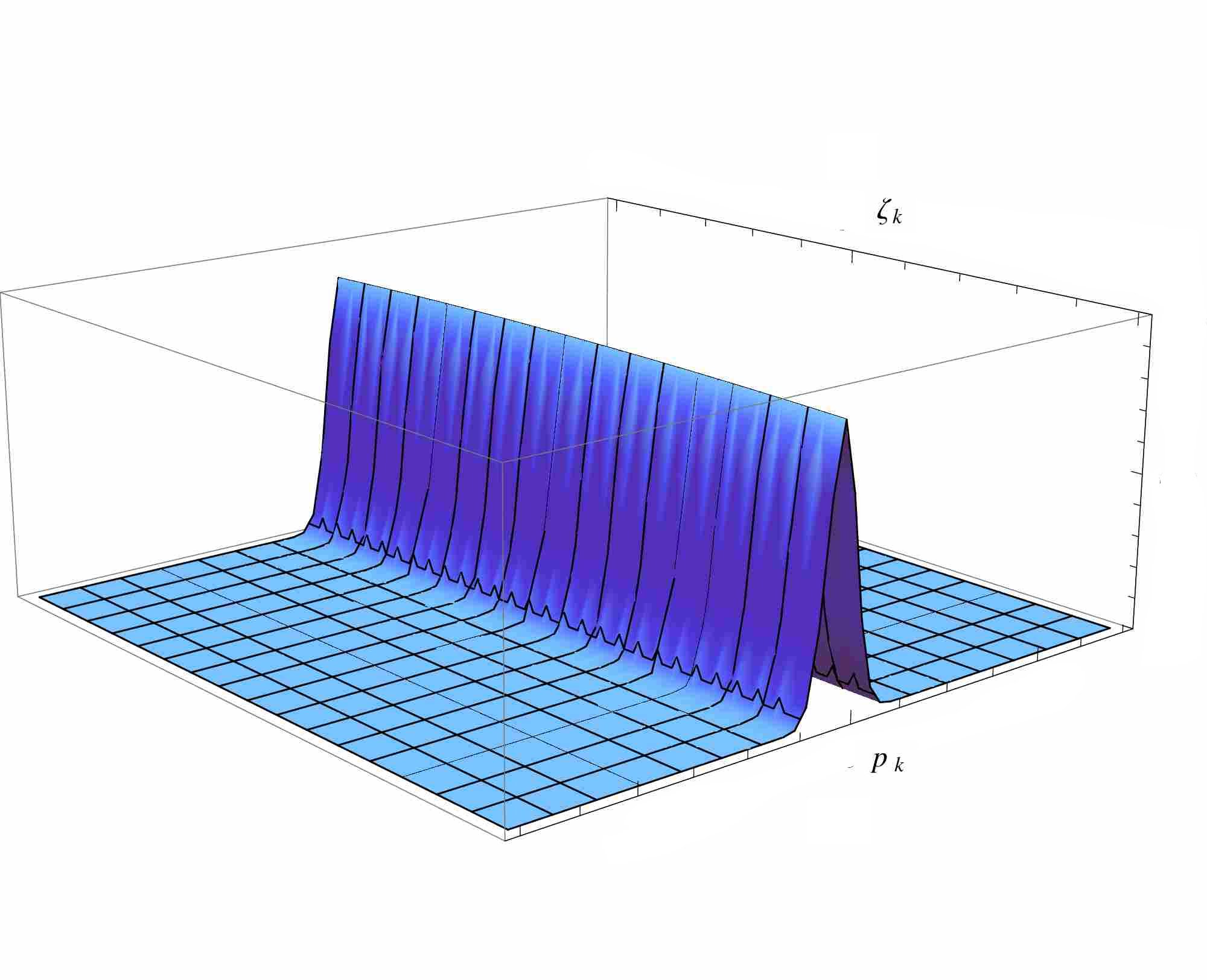
Figure 2: Plot of Wigner function in the case with constant $\gamma$ for $|r_{k}|=6.6$ and $\gamma=100$ showing high squeezing of a particular mode in the direction of momentum canonical to field variable

For the smaller modes for which $2\gamma/k^{2}\ll 1$ one has

$$\begin{array}[]{ccc}\kappa^{\rm R}\sim k,&&\kappa^{\rm I}\sim 0,\\ r_{k}^{\rm R}\sim\ln(-k\tau),&&r_{k}^{\rm I}\sim 0,\\ \phi_{k}^{\rm R}\sim\tan^{-1}\left(-\frac{1}{k\tau}\right),&&\phi_{k}^{\rm I}\sim 0,\end{array}$$ (113)

which yields

$${\rm Re}\,\Omega_{k}\approx 2k(-k\tau)^{2},$$ (114)

which also tends to zero as $-k\tau\rightarrow 0$ yielding squeezing in the direction of momentum for the smaller modes. In Fig. 2 we can see that despite the presence of a CSL correction with a constant $\gamma$ the Wigner function shows that the wavefunctional collapse has not taken place in the field eigenbasis and hence this scenario fails to explain the macro-objectification of the inflationary quantum fluctuations.

Now let us see the nature of power spectrum due to the effects of CSL mechanism. From Eqn. (65) we see that the scale-dependence of the power arises from the factor $a^{2}{\rm Re}\,\Omega_{k}$. Also from the above discussion we see that ${\rm Re}\,\Omega_{k}$ depends upon time $\tau$ for both long and short modes making the power spectrum time-dependent which is quite contrary to a generic inflationary scenario. This phenomenon has also been observed in Martin:2012pe where the authors have evaluated the power at the end of inflation. Following the same method as in Martin:2012pe we rewrite $-k\tau$ as

$$-k\tau=\frac{k}{k_{0}}e^{-\Delta N},$$ (115)

where $k_{0}$ is the comoving wave number of the mode which is at the horizon today $k_{0}=a_{0}H_{0}$ and $\Delta N$ is the number of e-foldings the mode $k$ has spent outside the Hubble radius during inflation and thus $\Delta N\approx 50-60$ for observationally relevant modes. It must be noted that it is not obvious in such a scenario whether the power spectrum calculated at the end of inflation would be the same at recombination. But as these modes are superhorizon at the end of inflation, one can expect the causal physics after inflation to not affect these modes considerably.

Hence for shorter modes we have $a^{2}{\rm Re}\,\Omega_{k}=2k^{3}$ which yields the power spectrum using Eqn. (65) as

$$\mathcal{P}_{\mathcal{R}}(k)=\frac{1}{16\pi^{2}\epsilon M^{2}_{\rm Pl}},$$ (116)

which is a scale-invariant power spectrum. On the other hand for longer modes one gets $a^{2}{\rm Re}\,\Omega_{k}=2\gamma k_{0}e^{\Delta N}$ which yields a power spectrum

$$\mathcal{P}_{\mathcal{R}}(k)=\frac{k^{3}}{16\pi^{2}\epsilon M^{2}_{\rm Pl}\gamma k_{0}}e^{-\Delta N}.$$ (117)

We see that for longer modes the power is scale-dependent $(\mathcal{P}_{\mathcal{R}}(k)\propto k^{3})$ which is not in accordance with the observations. Hence it has been suggested in Martin:2012pe that these modes which are scale-dependent due to the effects of CSL mechanism are still outside the horizon and thus observationally irrelevant. However in this way the observationally relevant modes will be the ones least affected by CSL and hence it will not be appropriate to expect localization in field variables for these modes due to CSL. Thus if one calls for CSL-like mechanism to explain the classicalization of modes which are observationally relevant then the scale-dependence of the power spectrum is inevitable. But, it is interesting to note that in the constant $\gamma$ model one can consider $k-$dependent $\gamma$ (in which case all the above derivations hold true) which can cure such discrepancies in the power spectrum as we will see in the later section.

IV Effects of scale-dependent ‘CSL-like’ term on inflationary dynamics and squeezing of modes

In the previous sections we discussed the squeezing of modes in a generic inflationary scenario as well as in the scenario of Martin et al. where ‘CSL-like’ modifications to inflationary dynamics have been considered with a constant ‘CSL-like’ parameter $\gamma$. In both these cases we observed that the squeezing of superhorizon modes happens in the direction of momentum which fails to explain the macro-objectification of the modes observed in the field-direction. Also, the scenario of inflation with constant CSL-like term lacks one essential feature of CSL modifications to quantum mechanics - namely the ‘amplification mechanism’. As the CSL-like parameter $\gamma$ is introduced as a constant in the functional Schrödinger equation of mode functions (see Eqn. (80)) the rate of localization is the same for all modes, larger or shorter. On the contrary, in CSL-modified quantum mechanics larger objects (with larger mass) becomes classical faster (i.e. their wave-function collapses more rapidly) than shorter objects which helps keep the microscopic objects in the quantum domain over astronomical time-scales. Here mass of a system (or a particle while dealing with single-particle system) has been chosen consciously as the relevant parameter of efficient collapse. Such a choice is very natural and driven by our prior knowledge of quantum and classical systems which can be distinctly discriminated by their mass. In the same spirit, while applying CSL-like modification to inflationary dynamics to justify the macro-objectification of the superhorizon modes, one should expect the modes to behave more classically as they start crossing the horizon, which indicates that the CSL-like term $\gamma$ should discriminate between different modes according to their physical length scales and grow stronger as a mode starts crossing the horizon during inflation. Hence $\gamma$ should be a function of length scale (or equivalently of conformal time $\tau$). Such a choice of scale dependence of $\gamma$ is also a conscious selection which is based on our prior knowledge of quantum and classical fields which can be discriminated by their population density and we know that with increasing length scales modes become more and more populated. We will see further that similar to the case in standard inflation, the physical length scale $1/k\tau$ of a mode $k$ is related to the squeezing parameter $r_{k}$. Since $r_{k}$ itself is directly related to the expectation of occupancy in a particular mode Albrecht:1992kf in the standard inflationary scenario, it seems natural to expect amplification with respect to the physical size in the inflationary context as it will correspond to a large occupancy in that particular mode for which classical behavior is more natural both from standard QFT and non-relativistic CSL formalism viewpoint. We therefore propose a phenomenological ansatz for the form of $\gamma$ as

$$\gamma=\frac{\gamma_{0}(k)}{(-k\tau)^{\alpha}},$$ (118)

where $\alpha>0$ so that the effects of CSL-like terms dominate as the modes evolve to cross the horizon and become superhorizon. Secondly, in the deep subhorizon regime we want the modes to evolve through standard unitary evolution. Thus, any modification should be vanishingly small in the extreme subhorizon case in order to obtain the Bunch-Davies vacuum in that limit. The above mentioned form of $\gamma$ seems compatible with this requirement too.

This modification changes the evolution equations for $f_{k}$ as

$$f_{k}^{\prime\prime}+\left(\kappa^{2}-\frac{a^{\prime\prime}}{a}\right)f_{k}=0,$$ (119)

where $\kappa^{2}\equiv k^{2}-2i\gamma_{0}(k)(-k\tau)^{-\alpha}$ has now become time-dependent. Here too $f_{k}$ and $\bar{f}_{k}$ are two independent solutions of the above equation. Writing $f_{k}$ in terms of $u_{k}$ and $v_{k}$ as before (as given in Eqn. (91)) we see that now $u_{k}$ and $v_{k}$ satisfy the following evolution equations

$$u_{k}^{\prime} = -i\kappa u_{k}+\left(\frac{a^{\prime}}{a}+\frac{\kappa^{\prime}}{2\kappa}\right)\bar{v}_{k}\,,$$

$$v_{k}^{\prime} = -i\kappa v_{k}+\left(\frac{a^{\prime}}{a}+\frac{\kappa^{\prime}}{2\kappa}\right)\bar{u}_{k}\,,$$ (120)

which accordingly change the evolution equations of $r_{k},\phi_{k}$ and $\theta_{k}$ as

$$r_{k}^{\prime} = \left(\frac{a^{\prime}}{a}+\frac{\kappa^{\prime}}{2\kappa}\right)\cos{2\phi_{k}},$$

$$\phi_{k}^{\prime} = -\kappa-\left(\frac{a^{\prime}}{a}+\frac{\kappa^{\prime}}{2\kappa}\right)\coth{2r_{k}}\sin{2\phi_{k}},$$

$$\theta_{k}^{\prime} = \kappa+\left(\frac{a^{\prime}}{a}+\frac{\kappa^{\prime}}{2\kappa}\right)\sin 2\phi_{k}\tanh r_{k}$$ (121)

where $u_{k}$ and $v_{k}$ is parameterized in terms of $r_{k},\phi_{k}$ and $\theta_{k}$ as before (see Eqn. (92)). Rest will remain same as in the case for constant $\gamma$. One can also check using

$$\frac{\bar{f}_{k}^{\prime}}{\bar{f}_{k}}=\frac{\bar{u}_{k}^{\prime}+v_{k}^{\prime}}{\bar{u}_{k}+v_{k}}-\frac{1}{2}\frac{\kappa^{\prime}}{\kappa}$$ (122)

for time-dependent $\kappa$ and Eqn. (120) that the expression for $\rm{Re}\,\Omega_{k}$ also remains the same as given in the time-independent case. It is difficult to exactly solve these evolution equations and therefore we will try to solve for the squeezing parameters approximately as we did before in the case of constant $\gamma$.

IV.1 Approximate solutions for squeezing parameters

To solve the evolution equations of the squeezing parameters approximately we first assume that $r_{k}^{\rm R}\rightarrow-\infty$ as $(-k\tau)\rightarrow 0$ as we did before which yields $\coth(2r_{k})\rightarrow-1$ in this superhorizon limit. Also we note that in this limit

$$\left.\frac{\kappa^{\prime}}{2\kappa}\right|_{-k\tau\rightarrow 0}\sim\frac{\alpha}{4}\frac{k}{(-k\tau)}.$$ (123)

This also shows that $\alpha\rightarrow 0$ would retrieve the equations for constant $\gamma$ case. Thus the evolution equations for $r_{k}$ and $\phi_{k}$ simplify in the superhorizon limit as

$$r_{k}^{\prime} = -\frac{1}{\tau}\left(1+\frac{\alpha}{4}\right)\cos{2\phi_{k}},$$

$$\phi_{k}^{\prime} = -\kappa-\frac{1}{\tau}\left(1+\frac{\alpha}{4}\right)\sin{2\phi_{k}}.$$ (124)

Defining $y=-\kappa\tau$ as before the above two equations can be rewritten as

$$\frac{\partial r_{k}}{\partial y} = -\frac{B}{A}\frac{1}{y}\cos{2\phi_{k}},$$

$$\frac{\partial\phi_{k}}{\partial y} = \frac{1}{A}-\frac{B}{A}\frac{1}{y}\sin{2\phi_{k}},$$ (125)

where $A\equiv\left(1-\alpha/2\right)$ and $B\equiv\left(1+\alpha/4\right)$. Making the transformation $\tan\phi_{k}=\mathcal{F}_{k}(y)$ as before the equation for $\phi_{k}$ can be written as

$$A\frac{\partial{\mathcal{F}}_{k}}{\partial y}-{\mathcal{F}}_{k}^{2}+\frac{2B}{y}{\mathcal{F}}_{k}=1,$$ (126)

whose solution can be given in terms of Bessel functions of regular and modified kind as

$${\mathcal{F}}_{k}(y)=\frac{J_{\frac{1}{2}+\frac{B}{A}}\left(\frac{y}{A}\right)\sec{\frac{(A+B)\pi}{A}}+J_{-\frac{1}{2}-\frac{B}{A}}\left(\frac{y}{A}\right)(C+\tan{\frac{B\pi}{A}})}{Y_{\frac{1}{2}-\frac{B}{A}}\left(\frac{y}{A}\right)-CJ_{\frac{1}{2}-\frac{B}{A}}\left(\frac{y}{A}\right)}.$$ (127)

We notice at this point that in the super-horizon limit ($-k\tau\rightarrow 0$) with $2\gamma_{0}(k)/k^{2}\gg 1$ one has

$$y\sim(-k\tau)^{1-\frac{\alpha}{2}}\left(\frac{4\gamma_{0}^{2}(k)}{k^{4}}\right)^{1/4}\exp{\left[-\frac{i}{2}\tan^{-1}\left(\frac{2\gamma_{0}}{k^{2}(-k\tau)^{\alpha}}\right)\right]},$$ (128)

where $y\rightarrow 0$ as $-k\tau\rightarrow 0$ if $\alpha<2$. Thus considering $0<\alpha<2$ the solution for $\mathcal{F}_{k}$ simplifies in the superhorizon limit as

$$\left.{\mathcal{F}}_{k}(y)\right|_{y\rightarrow 0}\sim\frac{1+\alpha}{y},$$ (129)

yielding

$$\tan{\phi_{k}}\approx\frac{1+\alpha}{y}.$$ (130)

Putting this back in the evolution equation of $r_{k}$ gives

$$\frac{\partial r_{k}}{\partial y}\approx\frac{B}{A}\frac{1}{y},$$ (131)

which yields a solution for $r_{k}$ in the superhorizon limit as

$$r_{k}\approx\frac{B}{A}\ln{y}$$ (132)

Now, one can explicitly write the real and imaginary parts of $\kappa$, $r_{k}$ and $\phi_{k}$ in the superhorizon limit as

$$\kappa^{\rm R} = \sqrt{\gamma_{0}}(-k\tau)^{-\frac{\alpha}{2}}\,,$$

$$\kappa^{\rm I} = -\sqrt{\gamma_{0}}(-k\tau)^{-\frac{\alpha}{2}}\,,$$

$$r_{k}^{\rm R} = \ln\left((-k\tau)^{1+\frac{\alpha}{4}}\left(\frac{4\gamma_{0}^{2}}{k^{4}}\right)^{\frac{4+\alpha}{8(2-\alpha)}}\right),$$

$$r_{k}^{\rm I} = -\frac{4+\alpha}{(2-\alpha)}\frac{\pi}{8},$$

$$\tan(\phi_{k}^{\rm R}) = \frac{\sqrt{2}}{(-k\tau)^{1-\frac{\alpha}{2}}}\left(\frac{2\gamma_{0}}{k^{2}}\right)^{-\frac{1}{2}},$$

$$\tanh\left(\phi_{k}^{\rm I}\right) = \frac{(-k\tau)^{1-\frac{\alpha}{2}}}{\sqrt{2}}\left(\frac{2\gamma_{0}}{k^{2}}\right)^{\frac{1}{2}},$$ (133)

which shows that with $0<\alpha<2$ one has $r_{k}^{\rm R}\rightarrow-\infty$ as $-k\tau\rightarrow 0$ in the superhorizon limit. This again justifies the assumption we made at the beginning.

IV.2 Wigner function and the macro-objectification of the inflationary modes

With the solutions of the squeezing parameters in the superhorizon limit one now can determine the nature of the Wigner function and the direction of squeezing of the modes. As we discussed earlier, the squeezing of modes is determined by the variance of exponentials with field and momentum as its coefficients which is directly related to ${\rm Re}\,\Omega_{k}$. In the present case, where the CSL-like parameter $\gamma$ is time-dependent, the explicit form of ${\rm Re}\,\Omega_{k}$ can be given by the one in the case of constant $\gamma$ as given in Eqn. (104). Thus using the approximate superhorizon solutions of $\kappa$, $r_{k}$ and $\phi_{k}$ from Eqn. (133) one sees that in the limits $\alpha<2,|k\tau|\ll 1$ and $2\gamma_{0}/k^{2}\gg 1$ the numerator of ${\rm Re}\,\Omega_{k}$ becomes

$$\left[2\sqrt{\gamma_{0}(k)}(-k\tau)^{-\alpha/2}+\frac{4\sqrt{2}}{k}\gamma_{0}(k)(-k\tau)^{1-\alpha}\right]\cos{\left(\frac{4+\alpha}{4-2\alpha}\frac{\pi}{2}\right)}+\frac{2\left(\frac{4\gamma_{0}^{2}(k)}{k^{4}}\right)^{1/2}}{\left(\frac{4\gamma_{0}^{2}(k)}{k^{4}}\right)^{\frac{1}{2}\frac{4+\alpha}{4-2\alpha}}}\frac{k}{(-k\tau)^{1+3\alpha/2}}$$

$$-2\sqrt{\gamma_{0}(k)}\sin{\left(\frac{4+\alpha}{4-2\alpha}\frac{\pi}{2}\right)}(-k\tau)^{-\alpha/2}-4\sqrt{2\gamma_{0}(k)}\left(\frac{4\gamma_{0}^{2}(k)}{k^{4}}\right)^{\frac{1}{4}}\sin{\left(\frac{4+\alpha}{4-2\alpha}\frac{\pi}{2}\right)}(-k\tau)^{1-\alpha}$$

$$+4\sqrt{\gamma_{0}(k)}\frac{2\left(\frac{4\gamma_{0}^{2}(k)}{k^{4}}\right)^{1/2}}{\left(\frac{4\gamma_{0}^{2}(k)}{k^{4}}\right)^{\frac{1}{2}\frac{4+\alpha}{4-2\alpha}}}\frac{1}{(-k\tau)^{2\alpha}},$$

whose leading order dependence in $|k\tau|$ will be $(-k\tau)^{-1-3\alpha/2}$ in the range $0<\alpha<2$. Similarly in the above limit the denominator of ${\rm Re}\,\Omega_{k}$ would be

$$4\left(\frac{4\gamma_{0}^{2}(k)}{k^{4}}\right)^{1/4}(-k\tau)^{1-\frac{\alpha}{2}}\frac{1}{\sqrt{2}}\cos{\left(\frac{4+\alpha}{4-2\alpha}\frac{\pi}{2}\right)}+\frac{\left(2+4\left(\frac{4\gamma_{0}^{2}(k)}{k^{4}}\right)^{1/4}(-k\tau)^{1-\frac{\alpha}{2}}\frac{1}{\sqrt{2}}\right)}{\left(\frac{4\gamma_{0}^{2}(k)}{k^{4}}\right)^{\frac{1}{2}\frac{4+\alpha}{4-2\alpha}}}\frac{1}{2(-k\tau)^{2+\frac{\alpha}{2}}}$$

$$+2\left(1+2\left(\frac{4\gamma_{0}^{2}(k)}{k^{4}}\right)^{1/4}(-k\tau)^{1-\frac{\alpha}{2}}\frac{1}{\sqrt{2}}\right)\left(\frac{4\gamma_{0}^{2}(k)}{k^{4}}\right)^{\frac{1}{2}\frac{4+\alpha}{4-2\alpha}}\frac{1}{2(-k\tau)^{2+\frac{\alpha}{2}}},$$

whose leading order dependence in $|k\tau|$ will be $(-k\tau)^{-(2+\frac{\alpha}{2})}$. Therefore, the leading order behavior of ${\rm Re}\,\Omega_{k}$ on super-horizon scales would be

$${\rm Re}\,\Omega_{k}\approx\frac{k}{2}(-k\tau)^{1-\alpha}\left(\frac{2\gamma_{0}(k)}{k^{2}}\right).$$ (136)

One can now see that if $0<\alpha<1$ then ${\rm Re}\,\Omega_{k}\rightarrow 0$ as $-k\tau\rightarrow 0$ on superhorizon scales which yields a squeezing in the direction of momentum as the variance in this direction becomes very small which can be seen from Eqn. (68). This also happens in a generic inflationary scenario as well as in the case where CSL-like correction is done with a constant $\gamma$ and we see as before that such a case fails to explain the macro-objectification of the modes observed in various experiments.

But, the scenario becomes very interesting for the range of $\alpha$ where $1<\alpha<2$. In this particular range one notices that ${\rm Re}\,\Omega_{k}\rightarrow\infty$ as $-k\tau\rightarrow 0$ on superhorizon scales which yields a squeezing in the direction of MS field variable $\zeta_{k}$ as the variance in this direction would then become very small which can be seen from Eqn. (68).

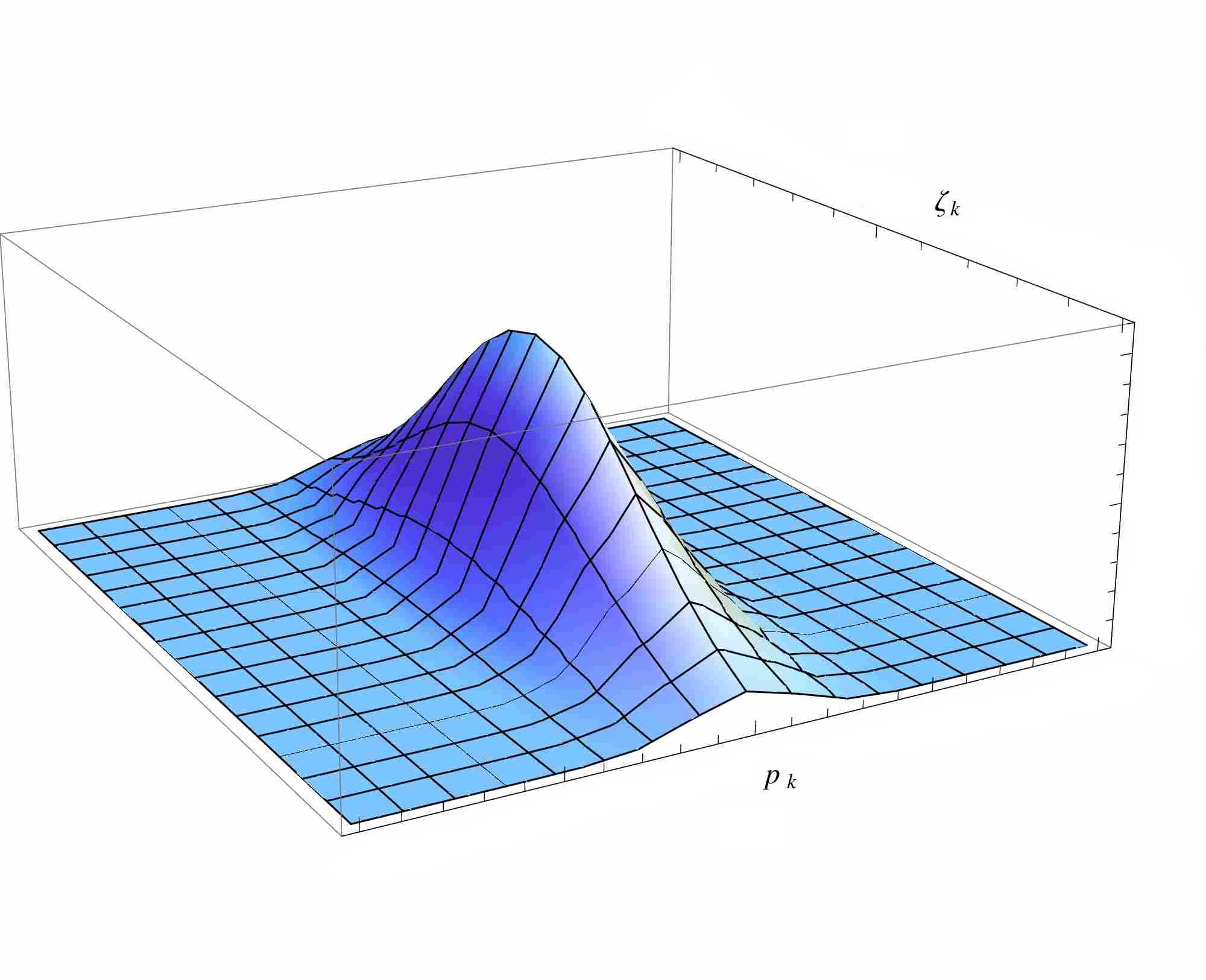
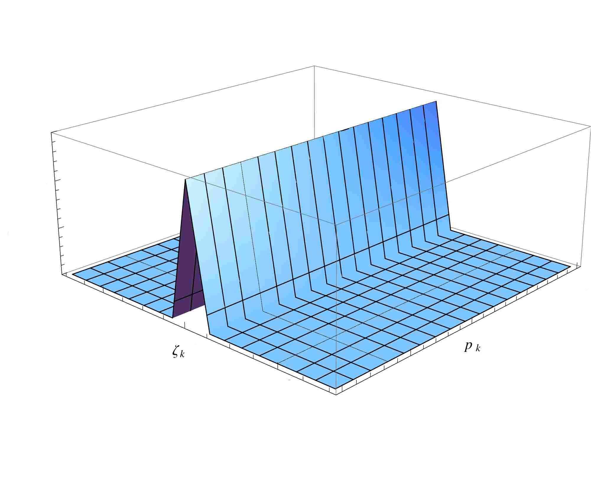
Figure 3: Plot of Wigner function for $\gamma=100$, $|r_{k}|=6.5$ and $\alpha=0.5$ for the plot in the left panel and $\gamma=100$, $|r_{k}|=6.2$ and $\alpha=1.5$ for the right panel figure. It shows high squeezing of a particular mode in the direction of field variable for the later case

In Fig. 3 we see that as long as we have $0<\alpha<1$, the squeezing remains in the direction of momentum whereas for the range $1<\alpha<2$ the direction of squeezing changes in favor of the field variable. This scenario is thus in accordance with the macro-objectification of the modes as suggested by cosmological observations without invoking requirement of decoherence and hence avoiding many-worlds scenario for explaining the observations.

IV.3 Obtaining the scale-invariant Power Spectrum

We previously saw in the case of constant $\gamma$ that introduction of CSL-like terms in the inflationary dynamics yield a scale-dependent power spectrum for the comoving curvature perturbations for the largest modes which contradicts the precise measurement of CMBR power spectrum of high-precision observations made by experiments like WMAP Hinshaw:2012fq and PLANCK Ade:2013uln . It is thus suggested in Martin:2012pe that these scale-dependent modes affected by constant CSL-like terms are still superhorizon at present day and thus are not related to these observations. The shorter modes on the other hand are not affected much by the CSL-like term $\gamma$ and thus can produce a scale-invariant power spectrum which is in accordance with the observations. This suggests that the constant $\gamma$ can spoil the observed scale invariance of the power spectrum and also suggests that CSL-like modifications to quantum theory are contradicted by inflationary dynamics. However, since now in our case $\gamma$ can depend upon $\tau$ as well as $k$ we can thus try to construct a scale-invariant power spectrum.

We see from Eqn. (65) that the scale-dependence of the power spectrum comes from the factor $k^{3}/(a^{2}{\rm Re}\,\Omega_{k})$. It is also to be noted that this factor depends upon $\tau$ yielding a time-dependent power spectrum as we also got while considering constant $\gamma$. In order to remove this $\tau$ dependence in the case of constant $\gamma$ the power spectrum was calculated at the end of inflation using Eqn. (115). We follow the same path here and calculate the power at the end of inflation.

We will be interested in the parameter regime where $1<\alpha<2$ as in this regime the macro-objectification of modes can be explained. In this regime ${\rm Re}\,\Omega_{k}$ can be approximately written in the superhorizon limit as

$${\rm Re}\,\Omega_{k}\approx\frac{k}{2}\left(\frac{2\gamma_{0}(k)}{k^{2}}\right)(-k\tau)^{1-\alpha}.$$ (137)

Thus in a de Sitter space the scale-dependence of the power spectrum would be

$$\frac{k^{3}}{a^{2}{\rm Re}\,\Omega_{k}}=\left(\frac{\gamma_{0}(k)}{k^{2}}\right)^{-1}(-k\tau)^{1+\alpha}=\left(\frac{\gamma_{0}(k)}{k^{2}}\right)^{-1}\left(\frac{k}{k_{0}}\right)^{1+\alpha}e^{-(1+\alpha)\Delta N},$$ (138)

where we have used Eqn. (115) for the last equality. In its present form we can see that if $\gamma_{0}$ has no dependence upon $k$ then the power would still be scale-dependent. But this can be fixed by fixing the scale dependence of $\gamma_{0}(k)$. In doing so we consider the form of $\gamma_{0}(k)$ as

$$\gamma_{0}(k)=\tilde{\gamma_{0}}\left(\frac{k}{k_{0}}\right)^{\beta},$$ (139)

where $\tilde{\gamma_{0}}$ is a constant with no dependence upon $k$ or $\tau$. With this we see that the scale-dependence of the power spectrum of the comoving curvature power spectrum would be

$$\mathcal{P}_{\mathcal{R}}(k)\propto k^{3+\alpha-\beta}$$ (140)

and thus by setting $\beta=3+\alpha$ one can get a scale-invariant power spectrum. As we are interested in the range $1<\alpha<2$, this sets a range for $\beta$ too as $4<\beta<5$. However, as correctly pointed out in Martin:2012pe the power spectrum remains time-dependent in such analysis, therefore, making any comparison of the power spectrum at the end of inflation with that at recombination non-trivial.

V Investigation of Phase Coherence of super-horizon fluctuations under CSL modifications

So far, while making modification to inflationary dynamics by adding CSL-like terms with either constant $\gamma$ or $\gamma$ which has $k$ and $\tau$ dependence, we were concerned about one observational consequence of inflationary dynamics: scale-invariance of the anisotropy spectrum of the precisely measured CMBR temperature fluctuations. On the other hand, it is also very important to note here that a generic inflationary scenario not only predicts a scale-invariant power spectrum, but also explains the existence of sharp peaks and troughs of the CMBR power spectrum which is caused by the coherent initial phases of all the Fourier modes of curvature perturbations at horizon re-entry corresponding to a given wave number. We previously showed (Eqn. (38) and discussion thereafter) how in a generic inflationary scenario the phase $\delta_{k}$ of the mode function $f_{k}$ freezes on super-horizon scales. In standard inflationary scenario we will see that it leads to freezing of the amplitude of the curvature perturbation on super-horizon scales. Upon re-entry the curvature perturbation begins to oscillate and it can be shown that all modes corresponding to a given wave number begin their oscillations with same initial phase (not to be confused with $\delta_{k}$) in that case, leading to a coherent interference to produce peaks and troughs in the CMBR power spectrum and a snapshot of it at the last scattering surface is what we observe today in different experiments such as WMAP Hinshaw:2012fq and PLANCK Ade:2013uln . But if all the Fourier modes of a given length scale had random phases, they would have interfered destructively to wash out all those sharp peaks and troughs of the CMBR spectrum to leave us simply with a flat spectrum Dodelson:2003ip ; Albrecht:1995bg .

We have seen before that modifying inflationary dynamics by CSL-like terms with constant $\gamma$ can yield a scale-dependent power spectrum for large scales which then contradicts with the observations. One can preferably keep these modes outside the horizon; thus making them observationally less important, but the smaller modes which explain a scale-invariant power spectrum are not much affected by CSL-like terms and thus their classicality cannot be explained by modification of inflationary dynamics with CSL mechanism. On the other hand we have seen that by making the CSL-like parameter $\gamma$ dependent upon $k$ and $\tau$ there exists a parameter range ($1<\alpha<2$ and $4<\beta<5$) where the macro-objectification of modes as well as a scale-invariant power spectrum can both be explained simultaneously. In this section we consider the phase coherence of the superhorizon modes and investigate whether inflationary dynamics modified by CSL-like mechanism is also in accordance with phase coherence or whether such CSL-like modifications of inflationary dynamics can spoil these patterns we observe in the CMBR spectrum and thus contradict the observations.

As argued above, phase coherence is related to the freezing of the amplitude of the curvature perturbation ($|{\mathcal{R}}_{k}|$) with respect to $\tau$. In standard inflation this is a trivial exercise to check by the means of the equation of motion for the variable $f_{k}$ by substituting $f_{k}$ as $R_{k}\exp{(i\delta_{k})}$, where $\delta_{k}$ carries the overall phase dependence, since $|{\mathcal{R}}_{k}|$ is given by the quantity $|f_{k}/a|$. The equations for its real and imaginary parts can be separated as Goswami:2010qu

$$\frac{R_{k}^{{}^{\prime\prime}}}{R_{k}}+\left[k^{2}-\frac{a^{{}^{\prime\prime}}}{a}-(\delta_{k}^{\prime})^{2}\right] = 0,$$ (141)

$$\delta_{k}^{{}^{\prime\prime}}+2\left(\frac{R_{k}^{\prime}}{R_{k}}\right)\delta_{k}^{\prime} = 0,$$ (142)

respectively. From Eqn. (142) we can see that $\delta_{k}^{\prime}=0$ is a fixed point of the equation and $\delta_{k}^{\prime}$ approaches this value asymptotically, i.e. for $|k\tau|\rightarrow 0$. Therefore, $R_{k}\rightarrow a$ and hence $|f_{k}/a|$ is constant resulting in the phenomenon of phase coherence.

But we note here that similar analysis of phase coherence in the case of CSL-modified inflationary dynamics would not hold as in such a case it is difficult to identify the parameter $f_{k}$ as the mode function as has been discussed before. But the requirement of phase coherence is related to freezing of amplitude of ${\mathcal{R}}_{k}$ on super horizon scales. We see from Eq. (65) that in Schrödinger picture analysis the amplitude of curvature perturbations varies as

$$|{\mathcal{R}}_{k}|\propto\frac{1}{\left(a^{2}{\rm Re}\,\Omega_{k}\right)^{\frac{1}{2}}}.$$ (143)

As the behavior of $a^{2}{\rm Re}\,\Omega_{k}$ is known for superhorizon modes for all the cases we discussed above, one can determine whether the amplitude of comoving curvature perturbation freezes on superhorizon scales in each such case or not. Let us analyze the phenomena of phase coherence case by case :

1. Constant $\gamma$ modification for larger modes :

We see from Eq. (109) that in such a case

$$\left(a^{2}{\rm Re\,}\Omega_{k}\right)^{\frac{1}{2}}\propto 1/\sqrt{-\tau},$$ (144)

which shows that

$$\frac{d|{\mathcal{R}}_{k}|}{d\tau}\propto 1/\sqrt{-\tau},$$ (145)

indicating that on superhorizon scales ($-k\tau\rightarrow 0$) the amplitude grows and would not freeze. Thus such modes can not lead to phase coherence of the CMBR spectrum. We recall that these modes also violate the scale invariance of the power spectrum and thus are inconsistent with observation.

2. Constant $\gamma$ modification for smaller modes :

In this case we see from Eq. (114) that $a^{2}{\rm Re}\,\Omega_{k}$ is a constant in $\tau$ which indicates that $|{\mathcal{R}}_{k}|$ does freeze on superhorizon scales and thus can give rise to the observed phase coherence of the CMBR spectrum. We also recall that such modes can yield a scale invariant spectrum and thus are observationally consistent. But as these modes are the ones least affected by the collapse operator and lead to a Wigner function squeezed in the momentum direction, rather than field direction, they do not satisfy the macro-objectivity criterion.

3. Modification with scale dependent $\gamma$ case :

We see from Eq. (136) that

$$\left(a^{2}{\rm Re}\,\Omega_{k}\right)^{\frac{1}{2}}\propto\frac{1}{(-\tau)^{\frac{1+\alpha}{2}}},$$ (146)

which yields the evolution of amplitude of curvature perturbations on superhorizon scales as

$$\frac{d|{\mathcal{R}}_{k}|}{d\tau}\propto(-\tau)^{(\alpha-1)/2}.$$ (147)

This indicates that for $\alpha>1$ the amplitude freezes on superhorizon scales and thus such modes can give rise to the observed phenomena of phase coherence in the CMBR spectrum. We also recall that this bound on $\alpha$ is also in accordance with macro-objectification of modes. Thus once $1<\alpha<2$ one can obtain macro-objectification of the modes and can also remain consistent with observations.

VI Conclusions

In this work we have analyzed an alternative scheme of dealing with the issue of classicalization of inflationary perturbations. This mechanism, although phenomenological at best, derives its motivation from a similar proposed modification to quantum theory, known as Continuous Spontaneous Localization, which addresses the issue of classicalization of macroscopic systems in non-relativistic physics. Although this scheme is not fully developed and still lacks a relativistic generalization, one can make an attempt to implement a similar stochastic correction in the Schrödinger representation of the field theoretic description. Martin et al. Martin:2012pe recently took a step in this direction by considering a CSL analog with constant $\gamma$ parameter. But it fails to capture the essential feature of such schemes, namely the amplification mechanism. Moreover, such a constant $\gamma$ model also leads to a distortion of the scale-invariance of power spectrum and so is in conflict with cosmological observations.

We take this approach further and consider a variable $\gamma$ model. We expect such a generalization to make the wavefunction evolve into one of the eigenfunctions of field variable. This should reflect itself in the squeezing of Wigner function along the field direction. The standard inflationary scenario squeezes the Wigner function along the momentum direction. Also, neither a small constant $\gamma$ nor any modification of the form of $\gamma(k)$ can yield squeezing in the field direction and hence fail to explain ‘single-outcome’ of the measured modes. Although one can take arbitrarily large $\gamma$ to cure for the squeezing direction, but our result shows that such models will still be at variance with phase coherence observed in the CMBR profile. However one can attempt a generalization where the CSL strength parameter is made time dependent so that the strength of correction will depend on the physical length scales of concerned modes. We see that although the most general class of ‘collapsing models’ will distort the power spectrum, there does exist a subfamily of these models which can generate scale invariance in accordance with the data without constraining the model further. It is to be noted here that in order to achieve scale-invariance of the spectrum we have exploited the arbitrariness of $k$ dependence of $\gamma$. It has so far no justification from the point of view of field theory and rather it is purely phenomenological. But until a relativistic generalization of CSL is achieved, this arbitrariness, we believe, is difficult to avoid.

In addition to scale-invariance of the power spectrum, the CMBR data also suggests the phase coherence of initial density perturbations which manifests itself in the acoustic peaks of the CMBR map. This observation also constrains one of the parameters, namely $\alpha$ to be greater than 1, which tallies with the requirement of macro-objectification. Thus such a model can account for cosmological observations such as scale-invariance of the primordial spectrum and the existence of acoustic peaks in the CMBR while providing a mechanism for macro-objectification. This also means that such bounds on the model parameter $\alpha$ should be respected by any suitable relativistic modification of CSL to be compatible with cosmology.

One important aspect of such CSL-like analysis in the Fourier basis is the non-conservation of energy. CSL formalism generically suffers with an ever-present non-conservation of energy Bassi:2003gd in the infinite temperature thermal bath model. As discussed in Martin:2012pe , a mode-by-mode analysis of inflationary fluctuations will make the expectation of the Hamiltonian diverge. For constant $\gamma$ model the divergence is $k^{3}$ while for our model the divergence is quite severe with a $k^{n}$ dependence where $n>6$. Such a strong increase in the energy density, even after regularization, can possibly lead to back-reaction and will be worth studying in future.

References

- (1) A. H. Guth, Phys. Rev. D 23, 347 (1981).
- (2) A. D. Linde, Phys. Lett. B 108, 389 (1982).
- (3) V. F. Mukhanov, H. A. Feldman and R. H. Brandenberger, Phys. Rept. 215, 203 (1992).
- (4) D. Baumann, arXiv:0907.5424 [hep-th].
- (5) G. Hinshaw, D. Larson, E. Komatsu, D. N. Spergel, C. L. Bennett, J. Dunkley, M. R. Nolta and M. Halpern et al., arXiv:1212.5226 [astro-ph.CO].
- (6) P. A. R. Ade et al. [Planck Collaboration], arXiv:1303.5082 [astro-ph.CO].
- (7) K. N. Abazajian et al. [SDSS Collaboration], Astrophys. J. Suppl. 182, 543 (2009) [arXiv:0812.0649 [astro-ph]].
- (8) S. Kanno and J. Soda, Phys. Rev. D 74, 063505 (2006) [hep-th/0604192].
- (9) A. De Felice and S. Tsujikawa, Living Rev. Rel. 13, 3 (2010) [arXiv:1002.4928 [gr-qc]].
- (10) P. Canate, P. Pearle and D. Sudarsky, arXiv:1211.3463 [gr-qc].
- (11) S. J. Landau, C. G. Scoccola and D. Sudarsky, Phys. Rev. D 85, 123001 (2012) [arXiv:1112.1830 [astro-ph.CO]].
- (12) A. Diez-Tejedor, G. Leon and D. Sudarsky, Gen. Rel. Grav. 44, 2965 (2012) [arXiv:1106.1176 [gr-qc]].
- (13) A. De Unanue and D. Sudarsky, Phys. Rev. D 78, 043510 (2008) [arXiv:0801.4702 [gr-qc]].
- (14) A. Perez, H. Sahlmann and D. Sudarsky, Class. Quant. Grav. 23, 2317 (2006) [gr-qc/0508100].
- (15) W. H. Zurek, Phys. Rev. D 24, 1516 (1981).
- (16) W. H. Zurek, Phys. Rev. D 26, 1862 (1982).
- (17) E. Joos and H. D. Zeh, Z. Phys. B 59, 223 (1985).
- (18) S. L. Adler, Stud. Hist. Philos. Mod. Phys. 34, 135 (2003) [quant-ph/0112095].
- (19) M. Schlosshauer, Rev. Mod. Phys. 76, 1267 (2004) [quant-ph/0312059].
- (20) H. Everett, Rev. Mod. Phys. 29, 454 (1957).
- (21) D. Bohm, Phys. Rev. 85, 166 (1952).
- (22) D. Bohm, Phys. Rev. 85, 180 (1952).
- (23) C. Kiefer and D. Polarski, Adv. Sci. Lett. 2, 164 (2009) [arXiv:0810.0087 [astro-ph]].
- (24) C. Kiefer, I. Lohmar, D. Polarski and A. A. Starobinsky, Class. Quant. Grav. 24, 1699 (2007) [astro-ph/0610700].
- (25) C. Kiefer, D. Polarski and A. A. Starobinsky, Int. J. Mod. Phys. D 7, 455 (1998) [gr-qc/9802003].
- (26) D. Polarski and A. A. Starobinsky, Class. Quant. Grav. 13, 377 (1996) [gr-qc/9504030].
- (27) J. Martin, V. Vennin and P. Peter, arXiv:1207.2086 [hep-th].
- (28) C. Kiefer and D. Polarski, Annalen Phys. 7, 137 (1998) [gr-qc/9805014].
- (29) A. Bassi and G. C. Ghirardi, Phys. Rept. 379, 257 (2003) [quant-ph/0302164].
- (30) A. Bassi, K. Lochan, S. Satin, T. P. Singh and H. Ulbricht, Rev. Mod. Phys. 85, 471 (2013) arXiv:1204.4325 [quant-ph].
- (31) A. Bassi and E. Ippoliti, Phys. Rev. A 69, 012105 (2004) [quant-ph/0307081].
- (32) S. L. Adler, J. Phys. A 38, 2729 (2005) [quant-ph/0411053].
- (33) S. L. Adler, A. Bassi and E. Ippoliti, J. Phys. A 38, 2715 (2005) [quant-ph/0407084].
- (34) P. M. Pearle, arXiv:0710.0567 [quant-ph].
- (35) P. Pearle, Found. Phys. 42, 4 (2012) [arXiv:1003.5582 [gr-qc]].
- (36) K. Lochan, S. Das and A. Bassi, Phys. Rev. D 86, 065016 (2012) [arXiv:1206.4425 [astro-ph.CO]].
- (37) P. M. Pearle and A. Valentini, quant-ph/0506115.
- (38) P. M. Pearle, Phys. Rev. D 13, 857 (1976).
- (39) G. C. Ghirardi, A. Rimini and T. Weber, Phys. Rev. D 34, 470 (1986).
- (40) P. M. Pearle, Phys. Rev. A 39, 2277 (1989).
- (41) G. C. Ghirardi, P. M. Pearle and A. Rimini, Phys. Rev. A 42, 78 (1990).
- (42) S. Weinberg, Phys. Rev. A 85, 062116 (2012) [arXiv:1109.6462 [quant-ph]].
- (43) S. Dodelson, AIP Conf. Proc. 689, 184 (2003) [hep-ph/0309057].
- (44) A. Albrecht, D. Coulson, P. Ferreira and J. Magueijo, Phys. Rev. Lett. 76, 1413 (1996) [astro-ph/9505030].
- (45) A. Albrecht, P. Ferreira, M. Joyce and T. Prokopec, Phys. Rev. D 50, 4807 (1994) [astro-ph/9303001].
- (46) L. Diosi, Phys. Rev. A 40, 1165 (1989).
- (47) A. Bassi, J. Phys. A 38, 3173 (2005)
- (48) A. Bassi and D. G. M. Salvetti, J. Phys. A 40, 9859 (2007)
- (49) B. Collett and P. Pearle Found. Phys. 33, 1495 (2003)
- (50) G. Goswami and T. Souradeep, Phys. Rev. D 83, 023526 (2011) [arXiv:1011.4914 [astro-ph.CO]].