Extended Object Tracking with
Random Hypersurface Models

Abstract

The Random Hypersurface Model (RHM) is introduced that allows for estimating a shape approximation of an extended object in addition to its kinematic state. An RHM represents the spatial extent by means of randomly scaled versions of the shape boundary. In doing so, the shape parameters and the measurements are related via a measurement equation that serves as the basis for a Gaussian state estimator. Specific estimators are derived for elliptic and star-convex shapes.

[t1]Draft accepted for publication in IEEE Transactions on Aerospace and Electronic Systems.

Chapter 0 Introduction

In target tracking applications Bar-Shalom2002 where the resolution of the sensor device is higher than the spatial extent of a target object, the usual point object assumption is not justified as several different points, i.e., measurement sources, on the target object may be resolved during a single scan (see Fig. 1). The resolved measurement sources typically vary from scan to scan and their locations depend on the shape of the object but also on further properties such as the surface or the target-to-sensor geometry. In this article, the basic idea is to approximate an extended object with a geometric shape such as an ellipse Gilholm2005 ; Koch2008 ; Fusion10_BaumNoack as depicted in Fig. 1. The tracking problem then consists of estimating the shape parameters in addition to the kinematic parameters. The locations of the measurement sources are not explicitly estimated. Reasonably, the shape of the target should be described as detailed as possible. However, when the measurement noise is rather high and only a few measurements are available, it may only be possible to infer a coarse shape approximation such as a circle.

The unknown locations of the measurement sources are usually modeled with a probability distribution whose mass is concentrated on the extended object (a so-called spatial distribution) Gilholm2005 ; G2005 . In general, no closed-form solutions for the likelihood function resulting from a spatial distribution model exist, so that Monte Carlo methods are frequently used for approximating the Bayesian filter solution Gilholm2005 ; G2005 ; Boers2006 ; Angelova2008 ; Petrov2011 ; Petrov2012a ; Petrov2012 . In case an elliptic extent is represented with a covariance matrix Koch2008 ; Feldmann2010 ; Degerman2011 ; Lan2012 ; Lan2012a ; Wieneke2012 , closed-form expressions can be derived with the help of random matrix theory. Spatial distributions have been embedded into the Probability Hypothesis Density (PHD) filter for tracking multiple extended objects Mahler2009 ; Granstrom2010 ; Orguner2011 ; Lundquist2011a ; Granstrom2012 . In Fusion09_Baum ; TAES_Baum it is proposed to drop all statistical assumptions on the measurement sources, which leads to combined set-theoretic and stochastic estimator.

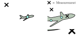
Figure 1: Shape approximation of an extended object with an ellipse.

1 Contributions

The main contribution is a novel systematic approach for modeling the unknown location of a measurement source on a spatially extended object called Random Hypersurface Model (RHM). The basic idea is to assume the measurement source to lie on a scaled version of the shape boundary, where the scaling factor is modeled as a random variable. In this manner, it is possible to form a suitable measurement equation that serves as the basis for constructing a Gaussian state estimator. In order to illustrate the novel approach, specific RHMs and corresponding Gaussian estimators are developed for ellipses and free-form star-convex shapes. To the best of our knowledge, this is the first extended object tracking method for explicitly estimating a free-form star-convex shape approximation. Actually, with this method, it is possible to track a target whose shape is a priori unknown and estimated from scratch over time.

Remark 1.

This article is based on SDF10_Baum ; Fusion11_Baum-RHM ; ISSPIT09_Baum ; Fusion10_BaumNoack ; CDC11_Baum ; Fusion10_BaumKlumpp ; IROS11_Baum ; SYSAES_Baum ; Diss13_Baum .

2 Overview

The remainder of this article is structured as follows: In the following section, the general probabilistic framework for extended object tracking is presented. The new target extent model called Random Hypersurface Model (RHM) is subsequently introduced in Section 2. Based on these models, a formal Bayes filter for extended object tracking is described in Section 3. Then, particular implementations of RHMs for ellipses (Section 4) and star-convex shapes (Section 5) are developed. Both shape representations are evaluated by means of typical extended object tracking scenarios in Section 6. This article is concluded in Section 7.

Chapter 1 Modeling Extended Targets

The state vector of the extended object at discrete time $k$ is represented with a random vector ${\boldsymbol{\underline{x}}}_{k}=\big{[}{\boldsymbol{\underline{m}}}^{T}_{k},({\boldsymbol{\underline{x}}}^{*}_{k})^{T},{\boldsymbol{\underline{p}}}_{k}^{T}\big{]}^{T}$ that consists of the target location ${\boldsymbol{\underline{m}}}_{k}$, a shape parameter vector ${\boldsymbol{\underline{p}}}_{k}$, and an optional vector ${\boldsymbol{\underline{x}}}^{*}_{k}$ for the kinematics, e.g., velocity. The shape parameter ${\boldsymbol{\underline{p}}}_{k}$ specifies a two-dimensional set that is denoted with ${\mathcal{S}}({\boldsymbol{\underline{p}}}_{k})\subset\mathds{R}^{2}$. For example, a circular shape can be specified by its radius ${\boldsymbol{r}}_{k}$, i.e., ${\boldsymbol{p}}^{\text{ci}}_{k}={\boldsymbol{r}}_{k}$ and the corresponding shape is ${\mathcal{S}}({\boldsymbol{p}}^{\text{ci}}_{k})=\{{\underline{z}}\;|\;{\underline{z}}\in\mathds{R}^{2}\text{ and }||{\underline{z}}||_{2}\leq{\boldsymbol{r}}_{k}\}$. Note that we focus on two-dimensional shapes. Nevertheless the concepts are also applicable to higher dimensional shapes in the same manner, see for example Fusion12_Faion-CylinderTracking .

1 Measurement Model

Figure 1: Measurement model for a single measurement.

At each time step $k$, a set of $n_{k}$ two-dimensional point measurements $\{\hat{{\underline{y}}}_{k,l}\}_{l=1}^{n_{k}}$ of the extended object is available. We assume the measurements to be mutually independent for given target state; hence, a measurement model for a single measurement is sufficient.

Extent Model

For a given state ${\boldsymbol{\underline{x}}}_{k}$, the target extent model specifies a single measurement source ${{\boldsymbol{\underline{z}}}}_{k,l}\in{\boldsymbol{\underline{m}}}_{k}+{\mathcal{S}}({\boldsymbol{\underline{p}}}_{k})$ on the extended object (see Fig. 1). In the following Section 2, we introduce the so-called Random Hypersurface Model for the target extent.

Sensor Model

For a given measurement source ${{\boldsymbol{\underline{z}}}}_{k,l}$, the sensor model specifies the measurement $\hat{{\underline{y}}}_{k,l}$. We focus on Cartesian point measurements corrupted with additive Gaussian noise according to

$$\hat{{\underline{y}}}_{k,l}={{\boldsymbol{\underline{z}}}}_{k,l}+{\boldsymbol{\underline{v}}}_{k,l}\enspace,$$ (1)

where the noise term ${\boldsymbol{\underline{v}}}_{k,l}$ is zero-mean white Gaussian noise with covariance matrix $\Sigma_{k,l}^{v}$.

2 Dynamic Model

In contrast to a point target, the temporal evolution of both the shape and kinematic parameters has to be modeled for an extended object. In this article, we focus on linear motion models according to

$${\boldsymbol{\underline{x}}}_{k+1}={{\mathbf{A}}}_{k}{\boldsymbol{\underline{x}}}_{k}+{\boldsymbol{\underline{w}}}_{k}\enspace,$$ (2)

where ${{\mathbf{A}}}_{k}$ is the system matrix and ${\boldsymbol{\underline{w}}}_{k}$ is white Gaussian system noise.

Chapter 2 Random Hypersurface Models

In this section, a new target extent model called Random Hypersurface Model (RHM) is introduced, which describes the location of a single measurement source in a star-convex region.

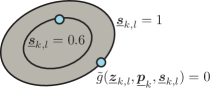
Figure 1: Random Hypersurface Model (RHM) for an ellipse.

Definition 1 (Star-Convexity).

A set ${\mathcal{S}}\subset\mathds{R}^{2}$ is star-convex with respect to the origin iff $\big{[}0,0\big{]}^{T}\in{\mathcal{S}}$ and each line segment from $\big{[}0,0\big{]}^{T}$ to any point in ${\mathcal{S}}$ is fully contained in ${\mathcal{S}}$.

1 Motivation: Implicit Measurement Equation

The objective is to form an equation that relates the measurement source with the shape parameters. When the measurement source ${{\boldsymbol{\underline{z}}}}_{k,l}$ lies on the boundary of the object, this is easy as the boundary is a closed curve (in general a hypersurface) that can be described by an implicit equation in the form $g({{\boldsymbol{\underline{z}}}}_{k,l},{\boldsymbol{\underline{p}}}_{k})=0$. However, the measurement sources may also lie in the interior of boundary. In order to cover the interior, the basic idea is to scale the object boundary as described in Fig. 1. As the corresponding scaling factor ${\boldsymbol{s}}_{k,l}\in[0,1]$ for a measurement source ${{\boldsymbol{\underline{z}}}}_{k,l}$ is unknown, we model it as a random variable and treat it as an additional noise term. By this means, we obtain the implicit relation

$$\tilde{g}({{\boldsymbol{\underline{z}}}}_{k,l},{\boldsymbol{\underline{p}}}_{k},{\boldsymbol{s}}_{k,l})=0$$ (1)

which forms, together with (1), an implicit measurement equation (note that $\tilde{g}({{\boldsymbol{\underline{z}}}}_{k,l},{\boldsymbol{\underline{p}}}_{k},1)=g({{\boldsymbol{\underline{z}}}}_{k,l},{\boldsymbol{\underline{p}}}_{k})$). In this sense, modeling a two-dimensional region is reduced to modeling a curve by means of the scaling factor.

2 Definition

According to the above motivation, RHMs assume that the measurement source is an element of a scaled version of the shape boundary, where the scaling factor is characterized by a particular probability distribution, i.e., the scaling factor is modeled as a one-dimensional random variable.

Definition 2 (Random Hypersurface Model (RHM)).

The measurement source ${{\boldsymbol{\underline{z}}}}_{k,l}\in{\boldsymbol{\underline{m}}}_{k}+{\mathcal{S}}({\boldsymbol{\underline{p}}}_{k})$ on an extended object with star-convex shape ${\mathcal{S}}({\boldsymbol{\underline{p}}}_{k})\subset\mathds{R}^{2}$ and center ${\boldsymbol{\underline{m}}}_{k}\in{\mathcal{S}}({\boldsymbol{\underline{p}}}_{k})$ is generated according to an RHM if

$${{\boldsymbol{\underline{z}}}}_{k,l}\in{\boldsymbol{\underline{m}}}_{k}+{\boldsymbol{s}}_{k,l}\cdot\bar{{\mathcal{S}}}({\boldsymbol{\underline{p}}}_{k})\enspace,$$

where $\bar{{\mathcal{S}}}({\boldsymbol{\underline{p}}}_{k})$ denotes the boundary of ${\mathcal{S}}({\boldsymbol{\underline{p}}}_{k})$ and ${\boldsymbol{s}}_{k,l}\in[0,1]$ is a one-dimensional random variable.

The restriction to star-convex shapes ensures that ${\mathcal{S}}({\boldsymbol{\underline{p}}}_{k})=\bigcup_{s\in[0,1]}\{s\cdot\bar{{\mathcal{S}}}({\boldsymbol{\underline{p}}}_{k})\}$. In fact, scaling the object boundary corresponds to a straight-line homotopy from the object center to the object boundary. Note that all scaling factors ${\boldsymbol{s}}_{k,l}$ are mutually independent because measurements are assumed to be mutually independent.

Definition 2 does not specify where the measurement source ${{\boldsymbol{\underline{z}}}}_{k,l}$ lies on the scaled boundary. In general, it is possible to consider it as an unknown fixed parameter (functional model) or to assume it to be drawn from a probability distribution (structural model). These two models are also widely-used in curve fitting Chernov2009 . For the structural model, an RHM becomes a spatial distribution model Gilholm2005 ; G2005 .

Remark 2.

The implicit representation motivated in Section 1 is based on the functional model. Probabilistic information about the location of a measurement source on the boundary is not explicitely encoded in the implicit function. The shape boundary can be written as

$$\bar{{\mathcal{S}}}({\boldsymbol{\underline{p}}}_{k})=\{{\underline{z}}\;|\;{\underline{z}}\in\mathds{R}^{2}\text{ and }g({\underline{z}},{\boldsymbol{\underline{p}}}_{k})=0\}\enspace,$$ (2)

and

$${\boldsymbol{s}}_{k,l}\cdot\bar{{\mathcal{S}}}({\boldsymbol{\underline{p}}}_{k})=\{{\underline{z}}\;|\;{\underline{z}}\in\mathds{R}^{2}\text{ and }\tilde{g}({\underline{z}},{\boldsymbol{\underline{p}}}_{k},{\boldsymbol{s}}_{k,l})=0\}\enspace$$ (3)

is the scaled shape boundary.

3 Probability Distribution of the Scaling Factor

The probability distribution of the scaling factor depends on the distribution of the measurement sources on the extended object. The following theorem says how the scaling factor is distributed in case the measurement sources are uniformly distributed on the surface of a two-dimensional extended object.

Theorem 1.

If the measurement source ${\boldsymbol{\underline{z}}}\in\mathds{R}^{2}$ is uniformly distributed over the star-convex region $\mathcal{S}\subset\mathds{R}^{2}$ with center $\big{[}0,0\big{]}^{T}$, the corresponding squared scaling factor is uniformly distributed on the interval $[0,1]$.

Proof.

The cumulative distribution function $F(s)$ of ${\boldsymbol{s}}$ turns out to be

$$F(s)=p\left({\boldsymbol{s}}\leq s\right)=p\left({\boldsymbol{\underline{z}}}\in s\cdot\mathcal{S}\right)=\frac{\text{Area}(s\cdot\mathcal{S})}{\text{Area}(\mathcal{S})}\;=\;s^{2}$$ (4)

for $s\in[0,1]$. Additionally, $F(s)=0$ for $s<0$ and $F(s)=1$ for $s>1$. The cumulative distribution of ${\boldsymbol{u}}:={\boldsymbol{s}}^{2}$ given by $F(u)=p\left({\boldsymbol{s}}\leq\sqrt{u}\right)$ is the cumulative distribution function of the uniform distribution on $[0,1]$. ∎

According to Theorem 1, it is reasonable choose a uniform distribution for the squared scaling factor.

4 General Procedure for Extended Object Tracking with RHMs

In order to derive a state estimator for an extended object based on an RHM, the following steps are to be performed:

• A suitable shape and a shape parameterization have to be determined.

• The implicit equation (1) has to be formed.

• A state estimator has to be derived based on the implicit measurement equation defined by (1) and (1).

Based upon the above steps, we will derive particular Gaussian estimators for ellipses and free-form star-convex shapes in this article.

Chapter 3 Formal Gaussian State Estimator for Extended Objects

In the following, the notation of a formal (Gaussian) Bayes filter for the state ${\boldsymbol{\underline{x}}}_{k}$ based on the previously discussed models is introduced. Particular implementations based on RHMs are presented in the next two sections.

We denote the probability density for the parameter vector ${\boldsymbol{\underline{x}}}_{k}$ after the incorporation of all measurements up to time step $k-1$ plus the measurements $\hat{{\underline{y}}}_{k,1},\ldots,\hat{{\underline{y}}}_{k,l}$ with $f_{l}({\underline{x}}_{k})$ for $0\leq l\leq n_{k}$. In this article, we focus on Gaussian state estimators so that all probability densities are approximated with Gaussians, i.e., $f_{l}({\underline{x}}_{k})\approx{\cal N}({\underline{x}}_{k}-{\underline{\mu}}^{x}_{k,l},\Sigma_{k,l}^{x})$, where ${\underline{\mu}}^{x}_{k,l}$ is the mean and $\Sigma_{k,l}^{x}$ the covariance matrix.

Time Update

The time update step predicts $f_{n_{k-1}}({\underline{x}}_{k-1})$ to the next time step, i.e., it determines $f_{0}({\underline{x}}_{k})$. As we focus on linear system models (2), the time update can be performed with the Kalman filter formulas, see for example Bar-Shalom2002 .

Measurement Update

The prediction $f_{0}({\underline{x}}_{k})$ is updated with the set of measurements $\{\hat{{\underline{y}}}_{k,l}\}_{l=1}^{n_{k}}$ according to Bayes’ rule. Because the measurement generation process is assumed to be independent for consecutive measurements, they can be incorporated recursively according to

$$f_{l}({\underline{x}}_{k})=\alpha_{k,l}\cdot f(\hat{{\underline{y}}}_{k,l}|{\underline{x}}_{k})\cdot f_{l-1}({\underline{x}}_{k})\text{ for }1\leq l\leq n_{k}\enspace,$$

where $f(\hat{{\underline{y}}}_{k,l}|{\underline{x}}_{k})$ is a single measurement likelihood function and $\alpha_{k,l}$ is a normalization factor.

Note that the order of the measurements for a particular time step is irrelevant, because they are generated independent. However, the processing order may matter if approximations are performed (see Remark 3).

Chapter 4 Elliptic Shapes

Elliptic shape approximations are highly relevant for real world applications as many targets are approximately elliptic. Even in case of high measurement noise and few available measurements, an elliptic shape approximation can be estimated. In this section, an implicit measurement equation is derived for elliptic shapes based on a RHM and subsequently a Gaussian state estimator is developed.

1 Parameterization of an Ellipse

An ellipse is determined by its center ${\boldsymbol{\underline{m}}}_{k}\in\mathds{R}^{2}$ and a positive semi-definite shape matrix ${{\mathbf{A}}}_{k}\in\mathds{R}^{2\times 2}$. Based on the Cholesky decomposition $({{\mathbf{A}}}_{k})^{-1}={{\mathbf{L}}}_{k}{{\mathbf{L}}}_{k}^{T}$, where

$${{\mathbf{L}}}_{k}:=\begin{bmatrix}{\boldsymbol{a}}_{k}&0\\ {\boldsymbol{c}}_{k}&{\boldsymbol{b}}_{k}\end{bmatrix}\enspace,$$ (1)

a suitable vectorized parameterization ${\boldsymbol{\underline{p}}}_{k}^{\text{el}}:=\begin{bmatrix}{\boldsymbol{a}}_{k},{\boldsymbol{b}}_{k},{\boldsymbol{c}}_{k}\end{bmatrix}^{T}$ of ${{\mathbf{A}}}_{k}$ can be defined. With ${\boldsymbol{\underline{x}}}_{k}^{\text{el}}:=\big{[}{\boldsymbol{\underline{m}}}^{T}_{k},({\boldsymbol{\underline{x}}}^{*}_{k})^{T},({\boldsymbol{\underline{p}}}_{k}^{\text{el}})^{T}\big{]}^{T}$, the implicit shape function becomes

$$g^{\text{el}}({{\boldsymbol{\underline{z}}}}_{k,l},{\boldsymbol{\underline{x}}}_{k}^{\text{el}}):=({{\boldsymbol{\underline{z}}}}_{k,l}-{\boldsymbol{\underline{m}}}_{k})^{T}\cdot{{\mathbf{A}}}_{k}^{-1}\cdot({{\boldsymbol{\underline{z}}}}_{k,l}-{\boldsymbol{\underline{m}}}_{k})-1\enspace.$$

2 Implicite Measurement Equation

Thanks to the chosen representation of an ellipse, the implicit function for the scaled version of $\bar{{\mathcal{S}}}({\boldsymbol{\underline{p}}}_{k}^{\text{el}})$ with scaling factor ${\boldsymbol{s}}_{k,l}$ turns out to be

$$\tilde{g}^{\text{el}}({{\boldsymbol{\underline{z}}}}_{k,l},{\boldsymbol{\underline{x}}}_{k}^{\text{el}},{\boldsymbol{s}}_{k,l}):=({{\boldsymbol{\underline{z}}}}_{k,l}-{\boldsymbol{\underline{m}}}_{k})^{T}\cdot{{\mathbf{A}}}_{k}^{-1}\cdot({{\boldsymbol{\underline{z}}}}_{k,l}-{\boldsymbol{\underline{m}}}_{k})-{\boldsymbol{s}}_{k,l}^{2}\enspace.$$ (2)

Equation (2) and (1) specify together an implicit measurement equation, which in this case coincides with the problem of fitting an ellipse to noisy data points plus the additional random scaling factor.

3 Gaussian State Estimator

Approaches based on the Kalman filter for state estimation with implicit measurement equations such as (2) and (1) are well-known in literature. Typically, the implicit measurement equation is linearized around the measurement and state in order to render it explicit, see for example Soatto1996 . Here, we propose to perform algebraic reformulations followed by a statistical linearization around the measurement source as described in the following. When (2) would be linear, we could rewrite the problem directly as an explicit measurement equation by plugging (1) into (2). As (2) is nonlinear, an exact reformulation is not possible. Nevertheless this reformulation can be performed approximately. For this purpose, the first step is to plug (1) into (2), i.e.,

$$\tilde{g}^{\text{el}}(\hat{{\underline{y}}}_{k,l},{\boldsymbol{\underline{x}}}_{k}^{\text{el}},{\boldsymbol{s}}_{k,l})=\tilde{g}({{\boldsymbol{\underline{z}}}}_{k,l}+{\boldsymbol{\underline{v}}}_{k,l},{\boldsymbol{\underline{p}}}_{k}^{\text{el}},{\boldsymbol{s}}_{k,l})\enspace.$$ (3)

After some minor simplifications of (3) and exploiting (2), the following measurement equation

$$h^{\text{el}}({\boldsymbol{\underline{x}}}_{k}^{\text{el}},{\boldsymbol{\underline{v}}}_{k,l},{\boldsymbol{s}}_{k,l},\hat{{\underline{y}}}_{k,l})=0\enspace$$ (4)

with a pseudo-measurement $0$ is obtained, where

$$h^{\text{el}}({\boldsymbol{\underline{x}}}_{k}^{\text{el}},{\boldsymbol{\underline{v}}}_{k,l},{\boldsymbol{s}}_{k,l},\hat{{\underline{y}}}_{k,l}):=\tilde{g}^{\text{el}}(\hat{{\underline{y}}}_{k,l},{\boldsymbol{\underline{p}}}_{k},{\boldsymbol{s}}_{k,l})-2({{\boldsymbol{\underline{z}}}}_{k,l}-{\boldsymbol{\underline{m}}}_{k})^{T}{{\mathbf{A}}}_{k}^{-1}{\boldsymbol{\underline{v}}}_{k,l}-{\boldsymbol{\underline{v}}}_{k,l}^{T}{{\mathbf{A}}}_{k}^{-1}{\boldsymbol{\underline{v}}}_{k,l}-{\boldsymbol{s}}_{k,l}^{2}\enspace$$ (5)

maps the state ${\boldsymbol{\underline{x}}}_{k}^{\text{el}}$, the measurement noise ${\boldsymbol{\underline{v}}}_{k,l}$, the scaling factor ${\boldsymbol{s}}_{k,l}$, and the measurement $\hat{{\underline{y}}}_{k,l}$ to the pseudo-measurement.

However, the unknown measurement source ${{\boldsymbol{\underline{z}}}}_{k,l}$ still occurs in (4). The basic idea here is to substitute ${{\boldsymbol{\underline{z}}}}_{k,l}-{\boldsymbol{\underline{m}}}_{k}$ in (4) with a proper point estimate. The easiest way to obtain a point estimate for ${{\boldsymbol{\underline{z}}}}_{k,l}-{\boldsymbol{\underline{m}}}_{k}$ is to consider the ellipse specified by the mean of the previous estimate, i.e., ${\underline{\mu}}^{p}_{k,l-1}$ and use the point with the smallest distance from the conic to the measurement $\hat{{\underline{y}}}_{k,l}$ as a point estimate for obtaining a point estimat for ${{\boldsymbol{\underline{z}}}}_{k,l}-{\boldsymbol{\underline{m}}}_{k}$.

The measurement equation (4) can directly be used within Gaussian state estimators such as the Unsented Kalman Filter (UKF) Julier_UnscentedFiltering or analytic moment calculation Fusion11_Baum , which essentially performs a statistical linearization of (4). More precisely, the joint density of the state and the predicted pseudo-measurement is approximated with a Gaussian. Then, the Kalman filtering Bar-Shalom2002 formulas can be used for calculating the updated estimate, i.e., given the previous estimate $f_{l-1}({\underline{x}}_{k})={\cal N}({\underline{x}}_{k}-{\underline{\mu}}^{x}_{k,l-1},\Sigma_{k,l-1}^{x})$, the updated estimate $f_{l}({\underline{x}}_{k})={\cal N}({\underline{x}}_{k}-{\underline{\mu}}^{x}_{k,l},\Sigma_{k,l}^{x})$ with the measurement $\hat{{\underline{y}}}_{k,l}$ results from the Kalman filter equations

$${\underline{\mu}}^{x}_{k,l} = {\underline{\mu}}^{x}_{k,l-1}+\Sigma_{k}^{xh}(\Sigma_{k}^{hh})^{-1}\left(0-{\underline{\mu}}^{h}_{k}\right)\enspace,$$ (6)

$$\Sigma_{k,l}^{x} = \Sigma_{k,l-1}^{x}-\Sigma_{k}^{xh}(\Sigma_{k}^{hh})^{-1}\Sigma_{k}^{hx}\enspace,$$ (7)

where $0$ is the predicted pseudo-measurement, $\Sigma_{k}^{xh}$ is the covariance between the pseudo-measurement and the state, and $\Sigma_{k}^{hh}$ is the variance of the predicted pseudo-measurement. In this manner, a statistical linearization around the measurement source is performed. At this point, it is important to note that ${\underline{\mu}}^{h}_{k}$ and $\Sigma_{k}^{xh}$ do not depend on the unknown measurement source ${{\boldsymbol{\underline{z}}}}_{k,l}$ and, hence, the error made due to substituting it with a point estimate is rather negligible.

Remark 3.

Due to the nonlinear measurement model and the performed approximations, the order of the measurement processing matters. However, we observed that the differences arising from different processing orders is rather negligible. Besides, it is possible to perform a batch processing of all measurements by means of stacking the single measurement functions (4). By this means, the estimation accuracy can be slightly increased.

Remark 4.

Due to the statistical linearization of the implicit measurement equation, approximation errors are introduced. As a consequence, the resulting estimation quality highly depends on the parameterization of the ellipse and of the particular form of $\tilde{g}^{\text{el}}(\hat{{\underline{y}}}_{k,l},{\boldsymbol{\underline{x}}}_{k}^{\text{el}},{\boldsymbol{s}}_{k,l})$. For example, we observed that multipliying both sides of (3) with $1/\operatorname{trace}\left({{\mathbf{L}}}_{k}{{\mathbf{L}}}_{k}^{T}\right)$ improves the estimation quality.

Remark 5.

Note that the actual likelihood function $f(\hat{{\underline{y}}}_{k,l}|{\underline{x}}_{k}^{\text{el}})$ can be derived from the measurement equation (4), however, it is not required explicitely when performing statistical linearization.

Chapter 5 Star-Convex Shapes

When the measurement noise is low compared to the target extent, it may be possible to extract more detailed shape information than an ellipse from the measurements. For this purpose, an RHM for estimating and tracking the parameters of a star-convex shape approximation is presented in the following. A detailed target shape approximation is of high value for many higher-level problems such as target classification, track management, and sensor management. Last but not least, a more detailed shape estimate results in a better estimation quality for the kinematic state of the target as it is a more precise model of the reality.

1 Parametrization of Star-Convex Shapes

A star-convex shape ${\mathcal{S}}({\boldsymbol{\underline{p}}}_{k}^{\text{sc}})$ can be represented in parametric form with the help of a radius function

(a) Star-convex shape.

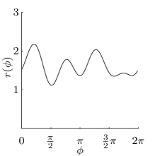
(b) Radius function.

Figure 1: Representation of a star-convex shape with a radius function.

$r({\boldsymbol{\underline{p}}}_{k}^{\text{sc}},\phi)$, which gives the distance from the object center to a contour point depending on the angle $\phi$ and a parameter vector ${\boldsymbol{\underline{p}}}_{k}^{\text{sc}}$ (see Fig. 1). A suitable (finite dimensional) parameterization ${\boldsymbol{\underline{p}}}_{k}^{\text{sc}}$ of a radius function is given by the first $N_{f}$ Fourier coefficients that define a Fourier series expansion Uensalan2001 ; Zhang2005 , i.e.,

$$r({\boldsymbol{\underline{p}}}_{k}^{\text{sc}},\phi)=\tfrac{1}{2}{\boldsymbol{a}}_{k}^{(0)}+\sum_{j=1\ldots N_{F}}\left({\boldsymbol{a}}_{k}^{(j)}\cos(j\phi)+{\boldsymbol{b}}_{k}^{(j)}\sin(j\phi)\right)={{\mathbf{R}}}(\phi)\cdot{\boldsymbol{\underline{p}}}_{k}^{\text{sc}}\enspace,$$

where

$${{\mathbf{R}}}(\phi) = [\tfrac{1}{2},\cos(\phi),\sin(\phi),\ldots,\cos(N_{F}\phi),\sin(N_{F}\phi)]\enspace,\text{ and }$$

$${\boldsymbol{\underline{p}}}_{k}^{\text{sc}} = \big{[}{\boldsymbol{a}}_{k}^{(0)},{\boldsymbol{a}}_{k}^{(1)},{\boldsymbol{b}}_{k}^{(1)},\ldots{\boldsymbol{a}}_{k}^{(N_{F})},{\boldsymbol{b}}_{k}^{(N_{F})}\big{]}^{T}\enspace.$$

Fourier coefficients with small indices encode information about the coarse features of the shape and Fourier coefficients with larger indices encode finer details.

2 Implicit Measurement Equation

With ${\boldsymbol{\underline{x}}}_{k}^{\text{sc}}:=\big{[}{\boldsymbol{\underline{m}}}^{T}_{k},({\boldsymbol{\underline{x}}}^{*}_{k})^{T},({\boldsymbol{\underline{p}}}_{k}^{\text{sc}})^{T}\big{]}^{T}$ and the implicit representation of star-convex curves Uensalan2001 , we obtain

$$g^{\text{sc}}({{\boldsymbol{\underline{z}}}}_{k,l},{\boldsymbol{\underline{x}}}_{k}^{\text{sc}})=||\boldsymbol{\underline{m}}-{{\boldsymbol{\underline{z}}}}_{k,l}||^{2}-r({\boldsymbol{\underline{p}}}_{k}^{\text{sc}},\measuredangle({\boldsymbol{m}}-{{\boldsymbol{\underline{z}}}}_{k,l}))^{2}\enspace,$$ (1)

where $\measuredangle({\boldsymbol{m}}-{{\boldsymbol{\underline{z}}}}_{k,l})$ denotes the angle between ${\boldsymbol{m}}-{{\boldsymbol{\underline{z}}}}_{k,l}$ and the $x$-axis. The scaled version of the shape boundary is specified by

$$\tilde{g}^{\text{sc}}({{\boldsymbol{\underline{z}}}}_{k,l},{\boldsymbol{\underline{x}}}_{k}^{\text{sc}},{\boldsymbol{s}}_{k,l})=||\boldsymbol{\underline{m}}-{{\boldsymbol{\underline{z}}}}_{k,l}||^{2}-\boldsymbol{s}_{k,l}^{2}\cdot r({\boldsymbol{\underline{p}}}_{k}^{\text{sc}},\measuredangle({\boldsymbol{m}}-{{\boldsymbol{\underline{z}}}}_{k,l}))^{2}\enspace,$$ (2)

Again, (2) specifies together with (1) an implicit measurement equation.

3 Bayesian State Estimator

A measurement equation can be derived by plugging (1) into (2)

$$\tilde{g}^{\text{sc}}(\hat{{\underline{y}}}_{k,l},{\boldsymbol{\underline{x}}}_{k}^{\text{sc}},{\boldsymbol{s}}_{k,l})=\tilde{g}({{\boldsymbol{\underline{z}}}}_{k,l}+{\boldsymbol{\underline{v}}}_{k,l},{\boldsymbol{\underline{p}}}_{k}^{\text{sc}},{\boldsymbol{s}}_{k,l})\enspace.$$ (3)

In order to avoid the treatment of uncertain angles, we propose to replace the angles in occurrences $r({\boldsymbol{\underline{p}}}_{k}^{\text{sc}},\cdot)$ with a point estimate $\hat{\phi}_{k,l}$, i.e., we assume $r({\boldsymbol{\underline{p}}}_{k}^{\text{sc}},\measuredangle({\boldsymbol{m}}-\hat{{\underline{y}}}_{k,l}))\approx r({\boldsymbol{\underline{p}}}_{k}^{\text{sc}},\measuredangle({\boldsymbol{m}}-({{\boldsymbol{\underline{z}}}}_{k,l}+{\boldsymbol{\underline{v}}}_{k,l}))\approx r({\boldsymbol{\underline{p}}}_{k}^{\text{sc}},\hat{\phi}_{k,l})$.

Remark 6.

A proper point estimate is given by the most likely angle $\phi_{k,l}$. In case of isotropic measurement noise, this point estimate $\phi_{k,l}$ is given by the angle between the vector from the current shape center estimate ${\underline{\mu}}^{m}_{k,l-1}$ to the measurement $\hat{{\underline{y}}}_{k,l}$ and the $x$-axis, i.e., $\hat{\phi}_{k,l}:=\measuredangle\big{(}\hat{{\underline{y}}}_{k,l}-{\underline{\mu}}^{m}_{k,l-1}\big{)}$.

Based on the point estimate and $\boldsymbol{\underline{m}_{k}}-{{\boldsymbol{\underline{z}}}}_{k,l}\approx{\boldsymbol{s}}_{k,l}\cdot{{\mathbf{R}}}(\hat{\phi}_{k,l})\cdot{\boldsymbol{\underline{p}}}_{k}^{\text{sc}}\cdot{\underline{e}}(\hat{\phi}_{k,l})$, where ${\underline{e}}(\hat{\phi}_{k,l}):=\big{[}\cos{\hat{\phi}_{k,l}},\sin{\hat{\phi}_{k,l}}\big{]}^{T}$, (3) can be simplified to the following measurement equation

$$h^{\text{sc}}({\boldsymbol{\underline{x}}}_{k},{\boldsymbol{\underline{v}}}_{k,l},{\boldsymbol{s}}_{k,l},\hat{{\underline{y}}}_{k,l})=0\enspace$$ (4)

with

$$h^{\text{sc}}({\boldsymbol{\underline{x}}}_{k}^{\text{sc}},{\boldsymbol{\underline{v}}}_{k,l},{\boldsymbol{s}}_{k,l},\hat{{\underline{y}}}_{k,l}):={\boldsymbol{s}}_{k,l}^{2}\cdot||{{\mathbf{R}}}(\hat{\phi}_{k,l})\cdot{\boldsymbol{\underline{p}}}_{k}^{\text{sc}}||^{2}+2{\boldsymbol{s}}_{k,l}{{\mathbf{R}}}(\hat{\phi}_{k,l}){\boldsymbol{\underline{p}}}_{k}^{\text{sc}}{\underline{e}}(\hat{\phi}_{k,l})^{T}{\boldsymbol{\underline{v}}}_{k,l}+||{\boldsymbol{\underline{v}}}_{k,l}||^{2}-||\hat{{\underline{y}}}_{k,l}-{\boldsymbol{\underline{m}}}_{k}||^{2}\enspace,$$

which maps the state ${\boldsymbol{\underline{x}}}_{k}^{\text{sc}}$, the measurement noise ${\boldsymbol{\underline{v}}}_{k,l}$, the scaling factor ${\boldsymbol{s}}_{k,l}$, and the measurement $\hat{{\underline{y}}}_{k,l}$ to a pseudo-measurement $0$.

Remark 7.

An alternative derivation of (4) based on the explicit representation of the shape with the radius function can be found in Fusion11_Baum .

For a given density $f_{l-1}({\underline{x}}_{k})={\cal N}({\underline{x}}_{k}-{\underline{\mu}}^{x}_{k,l-1},\Sigma_{k,l-1}^{x})$, the posterior density $f_{l}({\underline{x}}_{k})={\cal N}({\underline{x}}_{k}-{\underline{\mu}}^{x}_{k,l},\Sigma_{k,l}^{x})$ having received the measurement $\hat{{\underline{y}}}_{k,l}$ can be calculated with a Gaussian state estimator such as the UKF Julier_UnscentedFiltering or analytic moment calculation Fusion11_Baum for a closed-form measurement update. See also (6) and (7) in this context. Just as for ellipses, the order of the measurement processing matters (see the discussion in Remark 3).

Chapter 6 Evaluation

RHMs for elliptic and star-convex shapes are evaluated by means of both stationary and moving extended objects. For both elliptic shapes and star-convex shapes the UKF Julier_UnscentedFiltering is used for performing the measurement update. For elliptic shapes, the squared scaling factor is modeled as a Gaussian distribution with mean 0.5 and variance $1/12$ (i.e., the first two moments of a uniform distribution). For star-convex shapes, the scaling factor is modeled as Gaussian distribution with mean 0.7 and variance $0.06$.

1 Stationary Extended Target

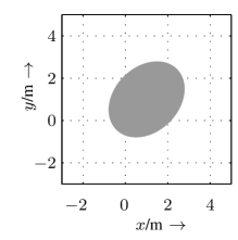
(a) Target 1: Elliptic shape.

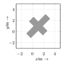
(b) Target 2: Aircraft-like shape.

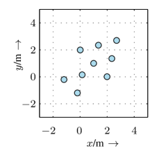
(c) Target 3: Group target.

Figure 1: Targets used for the evaluation.

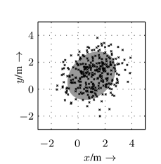
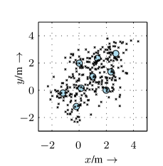
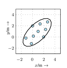
(a) Low noise level.

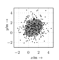
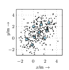
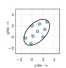
(b) Medium noise level.

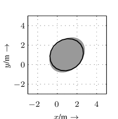
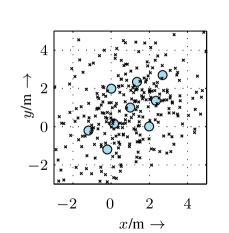
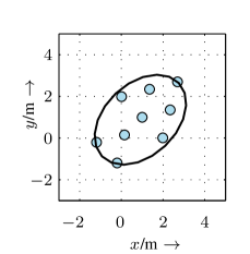
(c) High noise level.

Figure 2: Simulation results: Example measurements for a particular run and point estimates for the shape averaged over $20$ runs. Simulations are performed with low measurement noise level $\Sigma_{k,1}^{v}=\operatorname{diag}(0.6^{2},0.6^{2})$, medium measurement noise level $\Sigma_{k,1}^{v}=\operatorname{diag}(1,1)$, and high measurement noise level $\Sigma_{k,1}^{v}=\operatorname{diag}(1.4^{2},1.4^{2})$.

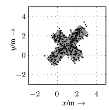
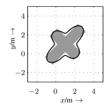
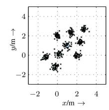
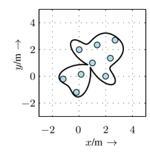
(a) Low noise level.

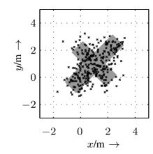
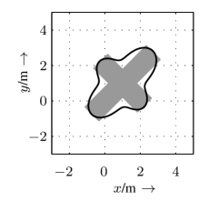
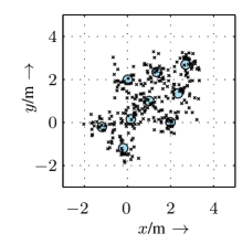
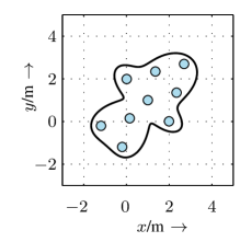
(b) Medium noise level.

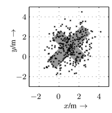
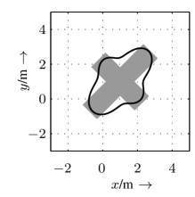
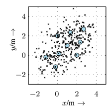
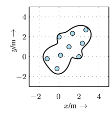
(c) High noise level.

Figure 3: Simulation results: Example measurements for a particular run and point estimates for the shape averaged over $20$ runs. Simulations are performed with low measurement noise level $\Sigma_{k,1}^{v}=\operatorname{diag}(0.3^{2},0.3^{2})$, medium measurement noise level $\Sigma_{k,1}^{v}=\operatorname{diag}(0.4^{2},0.4^{2})$, and high measurement noise level $\Sigma_{k,1}^{v}=\operatorname{diag}(0.6^{2},0.6^{2})$.

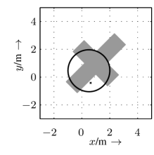
(a) First measurement.

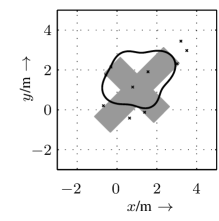
(b) 10 measurements.

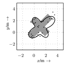
(c) 30 measurements.

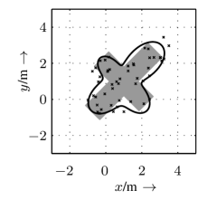
(d) 50 measurements.

Figure 4: Example run demonstrating the sequential incorporation of measurements (Noise level: $\Sigma_{k,1}^{v}=\operatorname{diag}(0.3,0.3)$).

In the first scenario, we consider an extended object with fixed position and shape. From the target, $300$ measurements are received sequentially, i.e., a single measurement per time step  ($n_{k}=1$). Simulations are performed with the three different target types depicted in Fig. 1, where measurement sources are drawn uniformly from the target surface/group members.

The parameters of the ellipse are a priori set to a Gaussian with mean $\big{[}0.5,0.5,1.6,1.6,0.6\big{]}^{T}$ and covariance matrix $\operatorname{diag}(3,3,0.5,0.5,0.5)$, i.e., an uncertain circle with radius $1.2$ and center $\big{[}0.5,0.5\big{]}^{T}$. For the star-convex shape approximation, $15$ Fourier coefficients are used, where the shape parameters are a priori set to a Gaussian with mean $\big{[}0.5,0.5,3,0,\ldots,0\big{]}^{T}$ and covariance matrix $\operatorname{diag}(0.7,0.7,0.1,0.1,\ldots,0.1)$, i.e., an uncertain circle with radius $1.5$ and center $\big{[}0.5,0.5\big{]}^{T}$.

The estimation results after the $300$ measurements are depicted in Fig. 2 and Fig. 3 for different measurement noise levels. The shape estimates are averaged over $20$ Monte-Carlo runs. In order to illustrate the magnitude of the measurement noise, the measurements of a particular run are also plotted. It is important to note that this is just done for visualization as the estimator incorporates the measurements recursively. Fig. 4 depicts a single example run for star-convex shapes in order to show the evolution of the shape estimates with an increasing number of measurements.

2 Moving Extended Object

In the second scenario, the aircraft-shaped target shown in Fig. 5a moves along the trajectory depicted in Fig. 5b. The measurement sources are drawn uniformly from the target surface. The magnitude of the measurement noise varies from measurement to measurement in order to simulate different sensors or different target-to-sensor geometries. The covariance matrix of the measurement noise is $\Sigma_{k,1}^{v}=\operatorname{diag}(0.2^{2},0.2^{2})$ with probability $0.75$ and $\Sigma_{k,1}^{v}=\operatorname{diag}(0.4^{2},0.4^{2})$ with probability $0.25$. The number of measurements received per time instant is given by $n_{k}=n^{*}_{k}+1$, where $n^{*}_{k}$ is a Poisson distributed random variable with mean $4$ for the ellipse and mean $7$ for the star-convex shape.

We employ a constant velocity model for the temporal evolution of the target center Bar-Shalom2002 and a random walk model for the shape parameters. Hence, the state vector to be tracked is ${\boldsymbol{\underline{x}}}_{k}=\big{[}{\boldsymbol{\underline{m}}}_{k},{\boldsymbol{\underline{m}}}^{v}_{k},{({\boldsymbol{\underline{p}}}_{k}^{\text{sc}})^{T}}\big{]}^{T}$, where ${\boldsymbol{\underline{m}}}_{k}$ is the center, ${\boldsymbol{\underline{m}}}^{v}_{k}$ is the velocity vector, and ${\boldsymbol{\underline{p}}}_{k}^{\text{sc}}$ are the shape parameters. As the center is assumed to evolve according to a constant velocity model, the system matrix in (2) is ${{\mathbf{A}}}_{k}=\operatorname{diag}({{\mathbf{A}}}^{cv}_{k},{{\mathbf{I}}}_{d})$, where ${{\mathbf{A}}}^{cv}_{k}=\begin{bmatrix}{{\mathbf{I}}}_{2}&T{{\mathbf{I}}}_{2}\\ 0&{{\mathbf{I}}}_{2}\end{bmatrix}$ with $T=1$ and ${{\mathbf{I}}}_{d}$ is the identity matrix with dimension $d=5$ for ellipses and $d=11$ for star-convex shapes. The system noise is zero-mean Gaussian noise with covariance matrix ${{\mathbf{C}}}_{k}^{w}=\operatorname{diag}(q_{1}\cdot{{\mathbf{I}}}_{d},{{\mathbf{C}}}_{k}^{cv})$ with ${{\mathbf{C}}}_{k}^{cv}=q_{2}\begin{bmatrix}\frac{T^{3}}{3}{{\mathbf{I}}}_{2}&\frac{T^{2}}{2}{{\mathbf{I}}}_{2}\\ \frac{T^{2}}{2}{{\mathbf{I}}}_{2}&T{{\mathbf{I}}}_{2}\end{bmatrix}$. For the ellipse, we have $q_{1}=0.0015$ and $q_{2}=0.005$. For the star-convex shape $q_{1}=0.0001$ and $q_{2}=0.003$.

The estimated shapes (averaged over $20$ time steps) are depicted in Fig. 6 and Fig. 7 for two snippets of the trajectory. The results show that the shape of the extended object is tracked precisely, even when the shape changes its orientation.

Note that in the simulations with elliptic shapes the number of measurements per time step is lower than for star-convex shapes. A star-convex shape approximation can only be extracted well in case the measurements carry enough information, i.e., enough measurements with rather low noise are available.

The example measurements in Fig. 6 and Fig. 7 also emphasize that naïve approaches for estimating a shape would be bound to fail, e.g., directly computing an enclosing shape of the measurements is infeasible because the measurements are noisy and only a couple of measurements are available per time step.

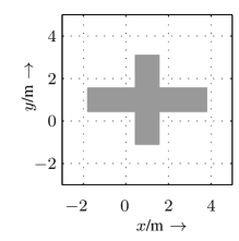
(a) Target shape.

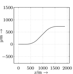
(b) Trajectory of the target.

Figure 5: Extended object and its trajectory.

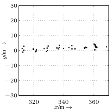
(a) Example measurements.

(b) Shape estimates.

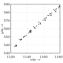
(c) Example measurements.

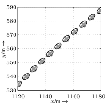
(d) Shape estimates.

Figure 6: Tracking an extended object with an RHM for ellipses: Example measurements from a particular run and average shape estimates.

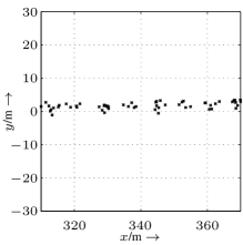
(a) Example measurements.

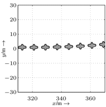
(b) Shape estimates.

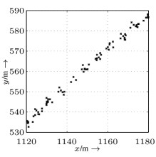
(c) Example measurements.

(d) Shape estimates.

Figure 7: Tracking an extended object with an RHM for star-convex shapes: Example measurements from a particular run and average shape estimates.

Chapter 7 Conclusions and Future Work

This article considered the problem of estimating a shape approximation of an extended object, which gives rise to several measurements from different spatially distributed measurement sources. For this purpose, a novel approach for modeling extended objects called Random Hypersurface Model (RHM) was introduced that allows to derive a functional relationship between the measurements and shape parameters. We presented particular RHMs for elliptic and free-form star-convex shapes and derived measurement equations for which standard Gaussian state estimators can be used. Nevertheless, estimating a detailed star-convex shape approximation is only possible when the measurement noise is rather low compared to target extent and enough measurements per time step are available. If this not the case, a basic shape such as an ellipse is more suitable. Hence, a mechanism for adapting the complexity of the used shape description is desired. The capability of estimating free-form shape approximations paves the way for new applications, e.g., classification based on the shape and group splitting detection.

References

- (1) Y. Bar-Shalom, T. Kirubarajan, and X.-R. Li, Estimation with Applications to Tracking and Navigation. New York, NY, USA: John Wiley & Sons, Inc., 2002.
- (2) K. Gilholm and D. Salmond, “Spatial Distribution Model for Tracking Extended Objects,” IEE Proceedings on Radar, Sonar and Navigation, vol. 152, no. 5, pp. 364–371, Oct. 2005.
- (3) J. W. Koch, “Bayesian Approach to Extended Object and Cluster Tracking using Random Matrices,” IEEE Transactions on Aerospace and Electronic Systems, vol. 44, no. 3, pp. 1042–1059, Jul. 2008.
- (4) M. Baum, B. Noack, and U. D. Hanebeck, “Extended Object and Group Tracking with Elliptic Random Hypersurface Models,” in Proceedings of the 13th International Conference on Information Fusion (Fusion 2010), Edinburgh, United Kingdom, Jul. 2010.
- (5) K. Gilholm, S. Godsill, S. Maskell, and D. Salmond, “Poisson Models for Extended Target and Group Tracking,” in SPIE: Signal and Data Processing of Small Targets, 2005.
- (6) Y. Boers, H. Driessen, J. Torstensson, M. Trieb, R. Karlsson, and F. Gustafsson, “Track-Before-Detect Algorithm for Tracking Extended Targets,” IEE Proceedings on Radar, Sonar and Navigation, vol. 153, no. 4, pp. 345–351, Aug. 2006.
- (7) D. Angelova and L. Mihaylova, “Extended Object Tracking Using Monte Carlo Methods,” IEEE Transactions on Signal Processing, vol. 56, no. 2, pp. 825–832, Feb. 2008.
- (8) N. Petrov, L. Mihaylova, A. Gning, and D. Angelova, “A Novel Sequential Monte Carlo Approach for Extended Object Tracking Based on Border Parameterisation,” in Proceedings of the 14th International Conference on Information Fusion (Fusion 2011), Chicago, Illinois, USA, Jul. 2011.
- (9) N. Petrov, A. Gning, L. Mihaylova, and D. Angelova, “Box Particle Filtering for Extended Object Tracking,” in 15th International Conference on Information Fusion (Fusion 2012). IEEE, jul 2012, pp. 82–89.
- (10) N. Petrov, L. Mihaylova, A. Gning, and D. Angelova, “Group Object Tracking with a Sequential Monte Carlo Method Based on a Parameterised Likelihood Function,” Monte Carlo Methods and Applications, 2012.
- (11) M. Feldmann, D. Fränken, and W. Koch, “Tracking of Extended Objects and Group Targets using Random Matrices,” IEEE Transactions on Signal Processing, vol. 59, no. 4, pp. 1409 –1420, 2011.
- (12) J. Degerman, J. Wintenby, and D. Svensson, “Extended Target Tracking using Principal Components,” in Proceedings of the 14th International Conference on Information Fusion (Fusion 2011), Chicago, Illinois, USA, Jul. 2011.
- (13) J. Lan and X. Rong Li, “Tracking of Extended Object or Target Group Using Random Matrix - Part I: New Model and Approach,” in 15th International Conference on Information Fusion (Fusion 2012), Jul. 2012, pp. 2177 –2184.
- (14) ——, “Tracking of Extended Object or Target Group Using Random Matrix -Part II: Irregular Object,” in 15th International Conference on Information Fusion (Fusion 2012), Jul. 2012, pp. 2185 –2192.
- (15) M. Wieneke and W. Koch, “A PMHT Approach for Extended Objects and Object Groups,” IEEE Transactions on Aerospace and Electronic Systems, vol. 48, no. 3, pp. 2349 –2370, july 2012.
- (16) R. P. S. Mahler, “PHD Filters for Nonstandard Targets, I: Extended Targets,” in Proceedings of the 12th International Conference on Information Fusion (Fusion 2009), Seattle, Washington, Jul. 2009.
- (17) K. Granström, C. Lundquist, and U. Orguner, “A Gaussian Mixture PHD filter for Extended Target Tracking,” in Proceedings of the 13th International Conference on Information Fusion (Fusion 2010), Edinburgh, Scotland, Jul. 2010.
- (18) U. Orguner, K. Granstrom, and C. Lundquist, “Extended Target Tracking with a Cardinalized Probability Hypothesis Density Filter,” in Proceedings of the 14th International Conference on Information Fusion (Fusion 2011), Chicago, Illinois, USA, Jul. 2011.
- (19) C. Lundquist, K. Granström, and U. Orguner, “Estimating the Shape of Targets with a PHD Filter,” in Proceedings of the International Conference on Information Fusion, Chicago, IL, USA, Jul. 2011.
- (20) K. Granström and U. Orguner, “A PHD Filter for Tracking Multiple Extended Targets Using Random Matrices,” IEEE Transactions on Signal Processing, vol. 60, no. 11, pp. 5657 –5671, Nov. 2012.
- (21) M. Baum and U. D. Hanebeck, “Extended Object Tracking based on Combined Set-Theoretic and Stochastic Fusion,” in Proceedings of the 12th International Conference on Information Fusion (Fusion 2009), Seattle, Washington, USA, Jul. 2009.
- (22) ——, “Extended Object Tracking Based on Set-Theoretic and Stochastic Fusion,” IEEE Transactions on Aerospace and Electronic Systems, vol. 48, no. 4, pp. 3103–3115, Oct. 2012.
- (23) M. Baum, M. Feldmann, D. Fränken, U. D. Hanebeck, and W. Koch, “Extended Object and Group Tracking: A Comparison of Random Matrices and Random Hypersurface Models,” in Proceedings of the IEEE ISIF Workshop on Sensor Data Fusion: Trends, Solutions, Applications (SDF 2010), Leipzig, Germany, Oct. 2010.
- (24) M. Baum and U. D. Hanebeck, “Shape Tracking of Extended Objects and Group Targets with Star-Convex RHMs,” in Proceedings of the 14th International Conference on Information Fusion (Fusion 2011), Chicago, Illinois, USA, Jul. 2011.
- (25) ——, “Random Hypersurface Models for Extended Object Tracking,” in Proceedings of the 9th IEEE International Symposium on Signal Processing and Information Technology (ISSPIT 2009), Ajman, United Arab Emirates, Dec. 2009.
- (26) M. Baum, B. Noack, and U. D. Hanebeck, “Random Hypersurface Mixture Models for Tracking Multiple Extended Objects,” in Proceedings of the 50th IEEE Conference on Decision and Control (CDC 2011), Orlando, Florida, USA, Dec. 2011.
- (27) M. Baum, V. Klumpp, and U. D. Hanebeck, “A Novel Bayesian Method for Fitting a Circle to Noisy Points,” in Proceedings of the 13th International Conference on Information Fusion (Fusion 2010), Edinburgh, United Kingdom, Jul. 2010.
- (28) M. Baum and U. D. Hanebeck, “Fitting Conics to Noisy Data Using Stochastic Linearization,” in Proceedings of the 2011 IEEE/RSJ International Conference on Intelligent Robots and Systems (IROS 2011), San Francisco, California, USA, Sep. 2011.
- (29) M. Baum, “Student Research Highlight: Simultaneous Tracking and Shape Estimation of Extended Targets,” IEEE Aerospace and Electronic Systems Magazine, vol. 27, no. 7, pp. 42–44, Jul. 2012.
- (30) ——, “Simultaneous Tracking and Shape Estimation of Extended Object (to appear),” Dissertation, Karlsruhe Institute of Technology (KIT), ISAS - Intelligent Sensor-Actuator-SystemsLaboratory, 2013.
- (31) F. Faion, M. Baum, and U. D. Hanebeck, “Tracking 3D Shapes in Noisy Point Clouds with Random Hypersurface Models,” in Proceedings of the 15th International Conference on Information Fusion (Fusion 2012), Singapore, Jul. 2012.
- (32) N. Chernov, Circular and Linear Regression: Fitting Circles and Lines by Least Squares. CRC Press, 2010.
- (33) S. Soatto, R. Frezza, and P. Perona, “Motion Estimation via Dynamic Vision,” IEEE Transactions on Automatic Control, vol. 41, no. 3, pp. 393–413, 1996.
- (34) S. J. Julier and J. K. Uhlmann, “Unscented Filtering and Nonlinear Estimation,” in Proceedings of the IEEE, vol. 92, no. 3, 2004, pp. 401–422.
- (35) M. Baum, B. Noack, F. Beutler, D. Itte, and U. D. Hanebeck, “Optimal Gaussian Filtering for Polynomial Systems Applied to Association-free Multi-Target Tracking,” in Proceedings of the 14th International Conference on Information Fusion (Fusion 2011), Chicago, Illinois, USA, Jul. 2011.
- (36) C. Ünsalan and A. Ercil, “Conversions Between Parametric and Implicit Forms Using Polar/Spherical Coordinate Representations,” Computer Vision and Image Understanding, vol. 81, no. 1, pp. 1 – 25, 2001.
- (37) D. Zhang and G. Lu, “Study and Evaluation of Different Fourier Methods for Image Retrieval,” Image and Vision Computing, vol. 23, no. 1, pp. 33 – 49, 2005.