Absence of superheating for ice $I_{h}$ with a free surface : a new method of determining the melting point of different water models.

Abstract

Cite as : C. Vega, M.Martin-Conde and A.Patrykiejew, Mol.Phys., 104, 3583, (2006).
Molecular dynamic simulations were performed for ice $I_{h}$ with a free surface. The simulations were carried out at several temperatures and each run lasted more than 7ns. At high temperatures the ice melts. It is demonstrated that the melting process starts at the surface and propagates to the bulk of the ice block. Already at the temperatures below the melting point, we observe a thin liquid layer at the ice surface, but the block of ice remains stable along the run. As soon as the temperature reaches the melting point the entire ice block melts. Our results demonstrate that, unlike in the case of conventional simulations in the NpT ensemble, overheating of the ice $I_{h}$ with a free surface does not occur. That allows to estimate the melting point of ice at zero pressure. We applied the method to the following models of water: SPC/E, TIP4P, TIP4P/Ew, TIP4P/Ice and TIP4P/2005, and found good agreement between the melting temperatures obtained by this procedure and the values obtained either from free energy calculations or from direct simulations of the ice/water interface.

I INTRODUCTION

For obvious reasons, liquid water has been the focus of thousands of simulation studies since the pioneering work of Barker and WattsBarker and Watts (1969) and Rahman and StillingerRahman and Stillinger (1971). However, simulation studies of the solid phases of water (ices) have been much more scarceMorse and Rice (1982); Báez and Clancy (1995); Ayala and Tchijov (2003); Baranyai et al. (2005); Rick (2005); Zheligovskaya and Malenkov (2006). There is a number of reasons to study solid and amorphous phases of water by computer simulation methods. First of all, the description of the phase diagram represents a major challenge for any potential model of water. Secondly, many experimental facts concerning ices and amorphous water are not completely understood and computer simulations could help in obtaining a molecular view of the process. Just to show a few examples, let us mention the nucleation of ice Radhakrishnan and Trout (2003); Matsumoto et al. (2002), the dynamics of solid-solid transitions, the possibility of liquid-liquid equilibria Poole et al. (1992); Mishima and Stanley (1998); Debenedetti (2003); Brovchenko et al. (2005), the speed and mechanism of crystal growth H. Nada and Furukawa (2004); Carignano et al. (2005) and the properties of ice at the free surfaceKroes (1992); Furukawa and H.Nada (1997); Nada and Furukawa (2000); Ikeda-Fukazawa and Kawamura (2004); Carignano et al. (2005).

Any researcher performing simulations of water must choose a potential model among the many now availableGuillot (2002); Chaplin ; Jorgensen and Tirado-Rives (2005). The most popular were developed in the eighties and are known as: TIP3PJorgensen et al. (1983) , TIP4PJorgensen et al. (1983); Bernal and Fowler (1933), TIP5PMahoney and Jorgensen (2000), SPCBerendsen et al. (1982) and SPC/E Berendsen et al. (1987). They were fitted to reproduce the properties of liquid water at room temperature and pressure. Before choosing a potential model of water it seems quite reasonable to ask about its ability to describe the phase diagram of water. Over the last decade, the vapour – liquid coexistence has been determined for several water models by using the Gibbs ensemble techniqueBoulougouris et al. (1998); Errington and Panagiotopoulos (1998); Lisal et al. (2001); Lísal et al. (2002); Chen et al. (2000); McGrath et al. (2006); Hernandez-Cobos et al. (2005); Vega et al. (2006). The critical properties of many water models are now known. However, the melting point of these models has been studied less often. Haymet et al. provided an estimate of the melting point of SPC, TIP4P and SPC/E water modelsKarim and Haymet (1988); Karim et al. (1990); Bryk and Haymet (2002), by performing simulations of the liquid-solid interface. The same approach has been followed recently by Wang et al.Wang et al. (2005) and by Nada and FurukawaNada and Furukawa (2005). By performing free energy calculations the melting points of the models SPC/E, TIP4P ,TIP5P and NvdENada and van der Eerden (2003) have been reportedBáez and Clancy (1995); Gao et al. (2000); Koyama et al. (2004); Vlot et al. (1999). It should be stated that estimates of the melting point of ice obtained by different authors and different techniques (or even by the same authors using different techniques) do not always agree, so it is still of interest to determine the melting point by as many different routes and methodologies as possible. Over the last few years, we have undertaken a systematic study of the solid phases of waterSanz et al. (2004a, b); Vega et al. (2005a, b). Firstly the phase diagrams for SPC/E and TIP4P models were obtained from free energy calculations Sanz et al. (2004a, b) by using the methodology proposed by Frenkel and LaddFrenkel and Ladd (1984), and extended to water models by Vega and Monson Vega and Monson (1998). Secondly, by using the Hamiltonian Gibbs-Duhem integrationSinger and Mumaugh (1990); Kofke (1993, 1998); Monson and Kofke (2000); Sturgeon and Laird (2000) the melting point of ice $I_{h}$ was obtained for several models of water Vega et al. (2005a). In these two last cases we used Monte Carlo methods and ”home-made” codes. Then, we applied a completely independent methodology, namely molecular dynamics methodFernandez et al. (2006), and used the GROMACS packageder Spoel et al. (2005) to perform direct simulations of fluid-solid coexistenceLadd and Woodcock (1977, 1978). It should be emphasized that we obtained excellent agreement between the normal melting temperatures $T_{m}$ ( i.e the melting temperature at the normal pressure of $p=1bar$ ) estimated by different routes. That was the case for the traditional SPC/E, TIP4P and TIP5P, and also for the new generation of models proposed just in the last two years, namely TIP4P/EwHorn et al. (2004), TIP4P/IceAbascal et al. (2005) and TIP4P/2005Abascal and Vega (2005), designed to improve the description of ices and water. Of course, each model predicts a different normal melting temperature, and the TIP4P/IceAbascal et al. (2005) model is known to perform best leading to $T_{m}=270\pm 2$K.

One may wonder why it is so cumbersome to determine the melting point of a water model. After all, melting points are determined easily in the lab conditions for many substances by simply heating the solid at constant pressure until it melts. Although liquids can be supercooled, solid can not be superheated as first stated by Bridgmann Bridgman (1912): ” It is impossible to superheat a crystalline phase with respect to the liquid. ”. For this reason there is in principle no risk in determining melting points by simply heating the solid until it melts. However, in computer simulations the situation is somewhat different. If conventional NpT simulations are performed for ice $I_{h}$ then it does not melt at $T_{m}$ but at a somewhat higher temperature McBride et al. (2005, 2004); Gay et al. (2002); Luo et al. (2004). It is worth mentioning that superheating has been also recently found experimentallyIglev et al. (2006); Schmeisser et al. (2006) for ice $I_{h}$ but only on a short time scale (about 200ps). The difference between the results of NpT simulations and those found in experiments (summarized in the Bridgman’s statement) is striking. However, there is a fundamental difference between experiments and NpT simulations of bulk solids. Whereas in experiments the ice (or a solid in general) must have a surface (or rather an interface at which it is in a contact with another phase; vapour or liquid), this interface is missing in conventional NpT simulations of bulk solids. When no interface is present ice must melt via bulk meltingde Donadio et al. (2005).

It is now commonly accepted that melting starts at the surface and already at the temperatures lower than the bulk melting point, solids exhibit a liquid-like layer at the surfaceAbraham (1981); van Der Veen et al. (1988); Dash (1989); Bienfait (1992); Broughton and Gilmer (1983). Different melting scenarios are possible depending on the behaviour of that liquid-like layer when the bulk melting temperature is approached from below. When the thickness of the liquid-like layer increases and finely diverges at $T=T_{m}$, i.e., when the solid is wetted by its own melt, one meets the so-called surface induced melting or just surface melting van Der Veen et al. (1988); Dash (1989); Frenken and van Pinxteren (1993); Nenov (1984); Frenken and van der Veen (1985). On the other hand when the liquid-like layer retains finite thickness up to $T=T_{m}$, i.e., when the melt does not wet completely the solid surface (partial wetting), one meets the case of surface nonmeltingCarnevali et al. (1987); Tartaglino et al. (2005). Both situations have been observed experimentally and found in computer simulations (for a review see that of Tartaglino et al.Tartaglino et al. (2005)). No matter which of the two above mentioned mechanisms occurs, the existence of an interface prevents the solid from overheating. One may therefore expect that the presence of a free surface at the ice sample, would turn the results of computer simulations back to normal, i.e. with melting occurring right at the bulk melting temperature.

The purpose of this paper is two-fold. On one hand we would like to check whether a piece of ice with a free surface can or not be superheated in computer simulation. As it will be shown shortly, the answer to this question is that when a free surface is present, superheating is suppressed in computer simulation, just the same as in experiment. Things go back to normal, and Bridgman’s statement holds again. Secondly the suppression of superheating means that there is another relatively straightforward way to determine the normal melting point. As it will be shown , the melting point obtained from the simulation of the free surface agrees with the estimates obtained by other routes. The problem of estimating melting points of water models seems solved, remaining uncertainties being of the order of about 3-4K.

II METHODOLOGY

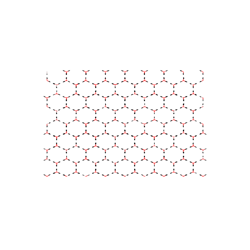
Figure 1: Initial configuration of the ice $I_{h}$ with 1024 molecules. The x axis goes from left to right so that the ice-vacuum interface is located at the right and left sides. The plane that can be seen is the basal plane. The plane exposed to the vacuum is the secondary prismatic plane.

Let us first describe the procedure used to get the initial configuration. Although the ice $I_{h}$ is hexagonal, it is possible to use an orthorrombic unit cellPetrenko and Whitworth (1999). It was with this orthorrombic unit cell that we generated the initial slab of ice. In ice $I_{h}$, protons are disordered whereas still fulfilling the Bernal-Fowler rules Bernal and Fowler (1933); Pauling (1935). We used the algorithm of Buch et al.Buch et al. (1998) to obtain an initial configuration with proton disorder and almost zero dipole moment (less than 0.1 Debye). This initial configuration contained 1024 molecules of water and fulfilled the Bernal Fowler rules. The dimensions of the ice sample were $36$  Å  x $31$  Å x $29$  Å . In oreder to equilibrate the solid, NpT simulations of bulk ice $I_{h}$ were performed at zero pressure at each temperature of interest. We used the molecular dynamics package Gromacs (version 3.3)der Spoel et al. (2005). The time step was 1fs and the geometry of the water molecules was enforced using constraintsRyckaert et al. (1977); Berendsen and van Gusteren (1984). The Lennard-Jones of the potential (LJ) was truncated at 9.0 Å . Ewald sums were used to deal with electrostatics. The real part of the coulombic potential was truncated at 9.0 Å . The Fourier part of the Ewald sums was evaluated by using the Particle Mesh Ewald (PME) method of Essmann et al.Essmann et al. (1995). The width of the mesh was 1 Å and we used a fourth other polynomial. The temperature was kept by using a Nose-HooverNosé (1984); Hoover (1985) thermostat with a relaxation time of 2 ps. To keep the pressure constant, a Parrinello-Rahman barostatParrinello and Rahman (1981); Nosé and Klein (1983) was used. The relaxation time of the barostat was of 2 ps. The pressure of the barostat was set to zero. We used a Parrinello-Rahman barostat where all three sides of the simulation box were allowed to fluctuate independently. The angles were kept orthogonal during this NpT run, so that they were not modified with respect to the initial configuration. The use of a barostast allowing independent fluctuations of the lengths of the simulation box is important. In this way, the solid can attain the equilibrium unit cell for the considered model and thermodynamic conditions. It is not a good idea to impose the geometry of the unit cell. The system should rather determine it from NpT runs. Once the ice is equilibrated at zero pressure we proceed to generate the ice-vacuum interface. By convention, we shall assume in this paper that the x axis is perpendicular to the ice-vacuum interface. The ice-vacuum configuration was prepared by simply changing the box dimension in the x axis from its value ( around 36  Å ) to 100  Å  . As a result, the dimensions of the simulation box are now 100  Å x 31  Å x 29  Å (the y and z are approximate since the actual values were obtained from the NpT runs for each model and at any particular value of the temperature). The approximate area of the ice-vacuum interface was 31  Å x 29  Å (approximately). This is about 10 molecular diameters in each direction parallel to the interface. In this work we have chosen the x axis to be of the 12̄10 direction. In other words, the ice is exposing its prismatic secondary plane to the vacuum (i.e the 12̄10 plane). In fig.1 we show the initial configuration of a perfect ice as seen from the basal plane. More details regarding ther relation of the main planes of ice (basal, primary prismatic and secondary prismatic) to the hexagonal unit cell can be found in in figure 1 of the paper by Nada and Furukawa Nada and Furukawa (2005), in the paper by Carignano et al.Carignano et al. (2005) and also in the water web site of Chaplin Chaplin (2005). Obviously, the properties of the ice-vacuum interface depend on the crystal plane facing the solid-vacuum interface. In particular, the melting mechanism (surface melting or surface nonmelting) may depend on the structure of the surface plane. On the other hand, the melting temperature should not depend on the choice of the plane selected to form the ice-vacuum interface. Therefore, the choice of the prismatic secondary plane is a good as any other. The main advantage arises from the fact that for the ice-water interfaces it has been shown that the 12̄10 plane exhibits the fastest dynamics Nada and Furukawa (2005); Carignano et al. (2005). It is also a convenient face to make a visualization of the melting process. Once the ice-vacuum system was prepared, we performed relatively long NVT runs (the lengths was between 4ns and 14ns depending on the model and thermodynamic conditions). Since we have been using NVT molecular dynamics, the dimensions of the simulation box have been fixed, of course, unlike in the preceding NpT run.

III RESULTS

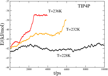
Figure 2: Total energy as a function of time obtained at several temperatures by performing MD simulations for a block of ice $I_{h}$ with a free surface. Results presented here correspond to the TIP4P model.

Let us first present results for the TIP4P model. In fig.2 the results of the total energy along the run are presented. As it is seen the total energy presents two different behaviours depending on the temperature. At high temperatures, the total energy of the system increases continuously and then reaches a plateau. The visualization of particle trajectories indicates that the block of ice melts and finally one obtains an slab of liquid in equilibrium with its vapour. The melting speed depends on the temperature but as it can be seen, close to the model melting point it is possible to melt the ice completely in about 6ns. The difference between the initial and the final energy is about 3.5 kJ/mol, indicating that the melting enthalpy is roughly of this order of magnitude. This is in reasonable agreement with the melting enthalpy of the TIP4P model, estimated in our previous workVega et al. (2005a) for the melting of bulk ice to bulk water, which was of about 4kJ/mol (the somewhat smaller value found here is due to the presence of the free surface ). Since the block of ice is of a thickness of about 36  Å , one can approximately state that an increase of energy by about 1 kJ/mol corresponds to a decrease of the thickness of the ice block by about 10  Å . Taking into account that we have two solid/vacuum interfaces, one at the right and the other at the left side of the ice block, it means roughly speaking an increase of the total energy by 1kJ/mol, which amounts to the formation of a liquid layer of about 5 Å (the argument is not elaborated but at least provides some orders of magnitude). The behaviour at low temperatures is different. At the beginning (first 1-2ns), there is an increase of the energy but after that the energy remains approximately constant, apart from the thermal fluctuations. The analysis of the configurations of the TIP4P at $T=228K$, shows that the increase of energy during the first 1ns is due to the formation of a thin liquid layer at the surface of ice, which may indicate the onset of surface melting, mentioned already in the Introduction, and first proposed by Faraday Rosenberg (2005).

We just recall that the term ”surface melting” usually represents the formation of a quasi-liquid layer (qll) on the surface of a solid at temperatures still below the melting point. The properties of this quasi-liquid layer are similar to, but not identical with, those of a bulk fluid under the same conditions. The thickness of the layer depends on the particular plane forming the solid-fluid interface and on the proximity to the melting point. It may diverge to infinity or stay finite as the temperature approaches $T_{m}$ from below. The surface melting of ice, has been found both in experiment (see Dash et al. (1995); Henson et al. (2005) and references therein ) and in computer computer simulation for several potential models of waterKroes (1992); Furukawa and H.Nada (1997); Nada and Furukawa (2000); Ikeda-Fukazawa and Kawamura (2004); Carignano et al. (2005). Some theories are also available to explain its originDash et al. (1995); Henson et al. (2005). One should note that the surface melting is an equilibrium phenomenon, leading to the lowering of the system free energy by replacing the ice-vacuum interface by the ice-liquid* and liquid*-vapour interfaces. By liquid* we mean a quasi-liquid layer of microscopic thickness. The existence of a quasi-liquid layer at temperatures below the melting point is not exclusive of ice, but it does also appear in simpler liquids such as metalsFrenken and van der Veen (1985); Pluis et al. (1987) or Lennard-Jones modelsAbraham (1981); Broughton and Gilmer (1983). The study of the quasi-liquid layer thickness by computer simulation is of interest by its own. This is so because different experimental techniques provide quite different values of its thicknessDash et al. (1995); Henson et al. (2005) and it is of interest to understand why this is the case. We expect to study that in future work. For the purpose of this work it is just enough to state, that at low temperatures a qll appears at the ice surface, provoking an increase of energy in the first 1-2ns of the run, but then the energy remains constant (with the normal thermal fluctuations) after this initial period. In that respect no signal of melting of the block of ice has been observed at the temperatures below $T_{m}$. By repeating the simulation at several temperatures it is possible to determine the lowest temperature at which the block of ice melts $T_{+}$, and the highest temperature at which it does not melt $T_{-}$. By taking the average of these two temperatures we obtain what we call $T_{s}=1/2(T_{+}+T_{-})$. For the length of the runs used (about 4-10ns) the typical difference between $T_{+}$ and $T_{-}$ is about 3-4K. It would be possible to reduce this temperature window by performing longer runs (of the order of hundred ns rather than of 10ns). However, taking into account that the current uncertainty in the estimations of the water melting point for different models obtained from the free energy calculations is just about 4K, the accuracy obtained by the runs of the length presented here seems to be quite sufficient. The crucial question now is, what $T_{s}$ actually is? How does $T_{s}$ compare with the melting point $T_{m}$? For the case of TIP4P, the melting point has been determined by several groups. From the free energy calculations we obtainedSanz et al. (2004a), $T_{m}=232K$. Starting from the melting point of the SPC/E model obtained by free energy calculations ( $T_{m}=215K$ ) and using Hamiltonian Gibbs-Duhem integration we obtained again $T_{m}=232K$ for the TIP4P modelVega et al. (2005a). Using free energy calculations, Koyama et al.Koyama et al. (2004) have obtained $T_{m}=229K$. From direct coexistence between the fluid and the solid phase we have obtained $T_{m}=228K$ Fernandez et al. (2006). From direct coexistence between the fluid and the solid Wang et al.Wang et al. (2005) have obtained $T_{m}=229K$. From the results presented in four different papers, each using different techniques and methods, it seems clear that the melting point of the TIP4P model is about $T=230(3)K$. This is also consistent with a corresponding states rule found by us recently. We have foundVega et al. (2006) that for TIP4P model the ratio of the melting point to the critical point temperatures is about 0.394. This estimate of the melting point temperature is consistent with the corresponding states rule and with the well known value of the critical temperature of the TIP4P modelLisal et al. (2001); Baranyai et al. (2006); Vega et al. (2006). The fact that there are some small discrepancies between different estimates is not surprising. They are due to the fact that long range forces are treated in a different way in different papers (truncation of the potential versus Ewald sums), different ice configurations (recall the issue of the proton disorder), different cutoff of the potential, as well as possible finite-size effects. Therefore, it can be stated with confidence that the melting point of the TIP4P is about $T=230(3)K$. The value of $T_{s}$ found in this work is $T_{s}=229(2)K$. The error in $T_{s}$ is mainly determined by the grid of temperature used, being the difference between $T_{+}$ and $T_{-}$ of about 4K, so that the error in $T_{s}$ is of about 2K. The obvious conclusion is that for the TIP4P model, and within the uncertainty of different estimates, $T_{s}$ is identical to $T_{m}$. In other words, overheating has been completely suppressed by the presence of a free surface.

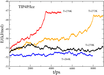
Figure 3: Total energy as a function of time obtained at several temperatures by performing MD simulations for a block of ice $I_{h}$ with a free surface. Results presented here correspond to the $TIP4P/Ice$ model.

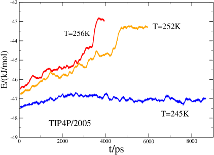
Figure 4: Total energy as a function of time obtained at several temperatures by performing MD simulations for a block of ice $I_{h}$ with a free surface. Results presented here correspond to the TIP4P/2005 model.

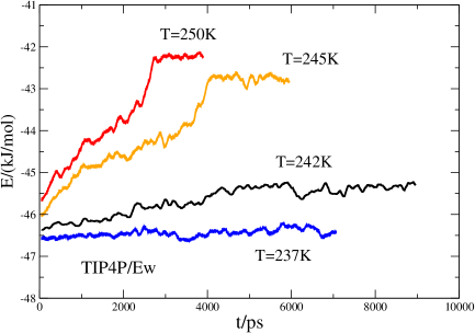
Figure 5: Total energy as a function of time obtained at several temperatures by performing MD simulations for a block of ice $I_{h}$ with a free surface. Results presented here correspond to the $TIP4P/Ew$ model.

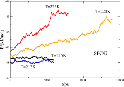
Figure 6: Total energy as a function of time obtained at several temperatures by performing MD simulations for a block of ice $I_{h}$ with a free surface. Results presented here correspond to the $SPC/E$ model.

In order to test the hypothesis, stating that $T_{s}$ and $T_{m}$ are identical, we have performed runs for other different models of water, namely the recently proposed TIP4P/IceAbascal et al. (2005) , TIP4P/2005Abascal and Vega (2005) , TIP4P/EwHorn et al. (2004) and the classical SPC/E model. Results of the runs for these models are presented in Figs.3-6 respectively. In Table I, the values of $T_{s}$ for different models are presented and compared with the values of $T_{m}$ obtained from a direct study of a fluid-solid coexistence, as well as from the Hamiltonian Gibbs-Duhem integration. As it can be seen, $T_{s}$ is identical to $T_{m}$, within the error bar. This result seems to be important, since it shows that the similarity between $T_{s}$ and $T_{m}$ is not a particular feature of the TIP4P model, but applies to any other model of water. The conclusion is that when a free surface is available overheating of the solid is suppressed, and the ice melts at the melting temperature, provided the length of the runs are sufficient (of the order of 10ns or larger), and the size of the ice block is sufficiently large, not smaller than about 3-4nm. To check whether this conclusion depends on the system size and/or of the face exposed to vacuum we have performed a run for the TIP4P/Ice model at a temperature of T=274K (higher than the melting point). In this particular case we used 1536 molecules and the plane at the ice-vacuum interface was the primary prismatic plane. The area of the interface was of about $27$  Å  x $30$  Å  . The width of the ice was of $63$  Å approximately. Again, complete melting of the sample was observed, indicating that the physics was not changed neither by a larger system nor by a different plane exposed. However, in this case it took about 25ns to melt the ice completely due to a larger size of the system and to slower dynamics.

A minor comment is in order here. The melting point obtained in our previous work $T_{m}$ corresponds to the melting point at the normal pressure $p=1bar$. However, $T_{s}$ was obtained in this work from simulations at zero pressure. Obviously, the melting temperature at zero pressure and at the pressure of one bar differ somewhat. In fact, for real water the difference is about 0.01K (i.e 273.16K for essentially zero pressure at the triple point versus 273.15K for $p=1bar$). For water models, the difference between the melting pressure at zero pressure and at $p=1bar$ is expected to be of the order of $1/(dp/dT)$. By using the values of $dp/dT$ reported in our previous workVega et al. (2005a) it can be seen that also for water models the difference between the melting temperatures at normal pressure and zero pressure should be of the order of about 0.01K (i.e quite small). In view of that, it it reasonable to identify $T_{m}$ with $T_{s}$. Still another comment is required with respect to our simulations of the ice-vacuum interface. In principle, when ice is exposed to vacuum at temperatures below the melting point there should be a solid-vapour equilibria. The vapour pressure of water at the triple point is quite low, namely $6\times 10^{-3}$ bar. The vapor pressure of TIP4P models at the triple point is fifty times smallerVega et al. (2006), about $1.3\times 10^{-4}$ bar. Although in principle one could determine the vapour pressure of ice by performing NVT runs of ice in contact with vacuum, this is not feasible in practice. In fact, for the lengths of the runs used in this paper we have never observed the sublimation of a single ice molecule into the vacuum (this of course should occur in very long runs, but since it is a rare event it was not observed in the runs of this work which lasted about 10ns). For this reason we prefer to say that $T_{s}$ was obtained at zero pressure, but it could be more appropriate to say that it was obtained at the sublimation pressure of the ice (which must be quite low anyway).

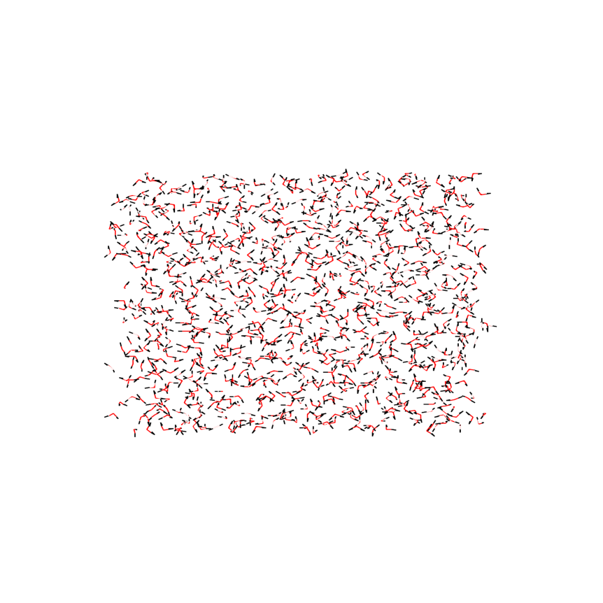
Figure 8: Instantaneous configuration of the TIP4P/Ice system at $T=276K$ at the end of the run after 5ns.

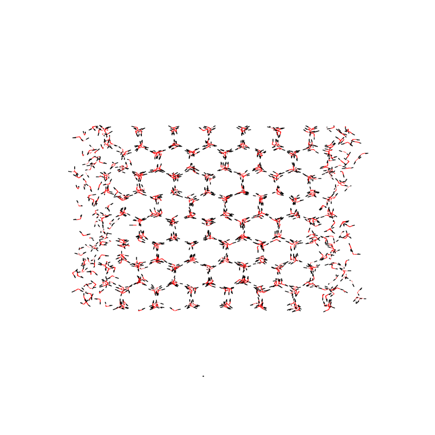
Figure 9: Instantaneous configuration of the TIP4P/Ice system at $T=264K$ at the end of a 8ns run. Although the temperature is well below the melting point of the model, a quasi-liquid layer is clearly present in the ice-vacuum interface.

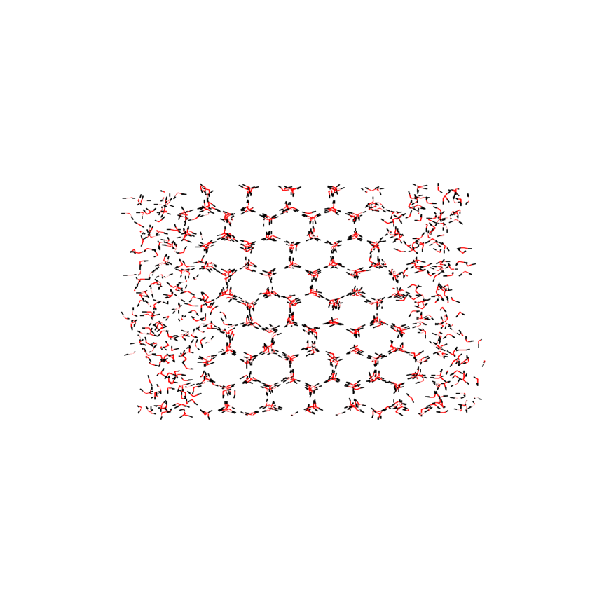
Figure 10: Instantaneous configuration of the TIP4P/Ice system at $T=270K$ at the end of a 9ns run. The temperature is just below the melting temperature of the model. A quasi-liquid layer is clearly present in the ice-vacuum interface.

It is interesting to see the mechanism of the melting process. We shall present results for the TIP4P/Ice at $T=276K$ (a temperature higher than the melting point of the model). In fig.7, a snapshot of the system after 1ns is shown. In fig.8, the final snapshot of the system after 5ns of run is shown. As shown in fig.8, the ice has melted completely after the run of 5ns. From the results given in Fig.7 it is also clear that the melting process starts at the surface and then propagates to the interior or the block of ice. We have analyzed the movies of all the runs and always found this to be the case. We have never observed the formation of a droplet of water in the interior part of the ice. We have always observed that the melting started at the surface and propagated to the interior part of the block of ice. One of the first methodologies proposed to estimate the melting point in computer simulations was the direct coexistence methodLadd and Woodcock (1977, 1978); Cape and Woodcock (1978). In this method, the solid is put into contact with the liquid at a certain temperature and pressure. If the temperature is higher than the melting temperature, the solid part of the sample will melt. If the temperature is lower than the melting temperature then the liquid will freeze. Regarding the ice-water interface, it has been investigated during the last fifteen years and estimates of the melting points for several water models have been given.Karim and Haymet (1988); Karim et al. (1990); Bryk and Haymet (2002, 2004); Wang et al. (2005); Nada and Furukawa (2005); Carignano et al. (2005); Fernandez et al. (2006). Recently, we have found that melting temperatures estimated from the direct coexistence method are in agreement with those obtained from free energy calculations. The presence of a ”nucleus” of ice in the sample, and of a ”nucleus” of liquid in the sample prevents the possibility of metastability. In other words, the presence of the two phases in the simulation sample from the very beginning avoids the possibility of metastability. The metastability is due to the fact that the formation of a nucleus of a new phase in the interior of another phase is an activated process. Although this is pretty clear, it was not so obvious what happened when the free surface of the solid was heated while exposed to vacuum. This work shows that also in this case superheating is suppressed. To prove further that a liquid layer is already present in the sample at temperatures well below the melting point, we present in fig.9 the final configuration (after a 8ns run) obtained for the TIP4P/Ice at a temperature well below the melting point of the model ($T=264K$). As it can be seen, a quasi liquid layer is already present in the system. In fig.10 the final configuration (after a 9ns run) obtained for the TIP4P/Ice at a temperature just below the melting temperature $T=270K$ is shown. It can be observed that the thickness of the quasi-liquid layer is larger now that at the lower temperature. The question whether the thickness of the liquid layer diverges when the melting point is approached (total wetting) or remains finite (partial wetting) should be studied in more detail. In any case figures 9 and 10 illustrate clearly the point that a quasi-liquid layer is already present in ice at temperatures below the melting point so that superheating is suppressed.

IV Conclusions

In this work, we have performed NVT Molecular Dynamics simulations of ice $I_{h}$ with a free surface. The ice was first equilibrated by performing NpT simulations at zero pressure. Simulations were then performed at several temperatures and runs lasted between 5 and 10ns. At temperatures below the melting point, the ice surface develops a thin liquid like layer (quasi liquid layer) of microscopic thickness. However, at temperatures above the melting point the ice melt, and does not exhibit any trace of overheating. In all cases, we have observed that the melting process starts at the surface and propagates to the interior of the material. We have estimated the melting point of ice $I_{h}$ for several water models, namely , TIP4P, TIP4P/Ice, TIP4P/2005, TIP4P/Ew, and SPC/E. Since the melting points of these water models had been evaluated previously (for ice $I_{h}$) by free energy calculations and by fluid-solid interface simulations, it is of interest to compare to the values obtained in this work. Excellent agreement has been found (see Table I) between previous estimates of $T_{m}$ and those obtained in this work from simulations of the free surface. Therefore, although it is possible to overheat ice in the usual BULK NpT simulationMcBride et al. (2005, 2004), the overheating does not seem to be possible as soon as the ice has a free surface. Although this phenomenon has been studied before for spherical fluidsTartaglino et al. (2005); Boutin et al. (1993), to the best of our knowledge this is the first time that the issue is addressed for such a complex fluid as water. As a bonus, one has a remarkably simple method to estimate the melting temperature of a water model: equilibrate first the material in an NpT run, and perform afterwards a long NVT run (of about 10ns or more). This is a long run but still within the capacity of current computers. Taking into account that estimating melting temperatures by free energy calculations is somewhat involved (although feasible) the existence of an alternative and simpler method is welcome. One should note that the method is probably not limited to water, but can also be used for other complex molecules. The method can be applied only when the following two conditions are met. Firstly, the melting of the system at temperatures above the melting point should be fast enough to be studied within a reasonable time by molecular simulations. Secondly, the liquid layer thickness at the temperatures below, but not too far from the melting point, should not be too large. Otherwise, the finite size of the sample may lead to the observation of complete melting already below the melting point. It should be pointed out that the procedure allows to estimate the zero pressure melting temperature, which should be very close to the normal melting point, but does not allow to estimate the fluid-solid coexistence at higher pressures.

Now, back to the classroom you may explain that the fluid-solid transition (in the absence of impurities leading to heterogeneous nucleation) occurs by the following mechanism: nucleation (of an embryo of the solid phase) and growth. Liquid water can be supercooled because the formation of an embryo is an activated process and that requires a certain amount of time to occur. You may now explain that melting occurs by the same mechanism: nucleation (of am embryo of the liquid phase) and growth. The point is that for ice with a free surface the embryo of the liquid phase is already there, at the surface of the solid. For this reason, the activation energy of forming the liquid embryo is zero and melting is just the growth of a new phase (i.e the propagation of the liquid layer from the surface to the interior of the solid). As stated by Bridgmann in his classical 1912 paper Bridgman (1912): ” It is impossible to superheat a crystalline phase with respect to the liquid. No good reason for this has ever been given, but no exception has ever been found, and it is coming to be regarded as a law of nature ”. We agree except for the absence of explanation for this behaviour. As stated by FrenkelFrenkel (1946); Dash et al. (1995) and suggested by TammannTammann (1910): ” It is well known that under ordinary conditions an overheating of a crystal, similar to the overheating of a liquid, is impossible. This peculiarity is connected with the fact that the melting of a crystal , which is kept at a homogeneous temperature, always begins on its free surface. The role of the latter must, accordingly, consist in lowering the activation energy, which is necessary for the formation of a flat embryo of the liquid phase, i.e. of a thin liquid film down to zero.”

V acknowledgements

It is a pleasure to acknowledge helpful discussions with Prof.J.L.F.Abascal, Dr.L.G.MacDowell, Dr.E.Sanz , Dr.C.McBride and R.G.Fernandez. This project has been financed by the grant FIS2004-06227-C02-02 of Direccion General de Investigacion, by the project S-0505/ESP/0299 of the Comunidad de Madrid and by the European Community under the grant No. MTDK-CT-2004-509249. One of us (CV) would like to thank the group of Molecular Modeling at the University of Lublin, and specially Andrzej Patrykiejew and Stefan Sokolowski for the hospitality during his stay in Lublin.

Table 1: Normal melting points $T_{m}$ of different water models as obtained from different methodologies. The column labeled as free energy correspond to the melting point either as obtained from free energy calculationsSanz et al. (2004a, b) (SPC/E and TIP4P) or from Hamiltonian Gibbs Duhem integrationVega et al. (2005a). (TIP4P/Ice, TIP4P/2005, TIP4P/Ew). The results of the column labeled as Solid-Liquid interface have been obtained from direct coexistence of the solid with the liquid Fernandez et al. (2006). The last column is the value of $T_{s}$ (which is just the average of the lowest temperature at which ice melts and the highest at which it does not melts) obtained from simulations of ice $I_{h}$ with a free interface. The similarity of $T_{s}$ and $T_{m}$ shows the absence of superheating for ice with a free surface.

Model	$T_{m}/K$ (Free energy)	$T_{m}/K$ (Solid-Liquid interface)	$T_{s}/K$ (this work)
TIP4P	232(4)	229(2)	230(2)
TIP4P/Ice	272(6)	268(2)	271(1)
TIP4P/2005	252(6)	249(2)	249(3)
TIP4P/Ew	245.5(6)	242(2)	243(2)
SPC/E	215(4)	213(2)	217(2)

Figure 7: Instantaneous configuration of the TIP4P/Ice system at $T=276K$ after 1ns run.

References

- Barker and Watts (1969) J. A. Barker and R. O. Watts, Chem. Phys. Lett. 3, 144 (1969).
- Rahman and Stillinger (1971) A. Rahman and F. H. Stillinger, J. Chem. Phys. 55, 3336 (1971).
- Morse and Rice (1982) M. D. Morse and S. A. Rice, J. Chem. Phys. 76, 650 (1982).
- Báez and Clancy (1995) L. A. Báez and P. Clancy, J. Chem. Phys. 103, 9744 (1995).
- Ayala and Tchijov (2003) R. B. Ayala and V. Tchijov, Canadian Journal of Physics 81, 11 (2003).
- Baranyai et al. (2005) A. Baranyai, A. Bartók, and A. A. Chialvo, J. Chem. Phys. 123, 54502 (2005).
- Rick (2005) S. W. Rick, J. Chem. Phys. 122, 094504 (2005).
- Zheligovskaya and Malenkov (2006) E. A. Zheligovskaya and G. G. Malenkov, Russian Chemical Reviews 75, 57 (2006).
- Radhakrishnan and Trout (2003) R. Radhakrishnan and B. Trout, J. Am. Chem. Soc. 125, 7743 (2003).
- Matsumoto et al. (2002) M. Matsumoto, S. Saito, and I. Ohmine, Nature 416, 409 (2002).
- Poole et al. (1992) P. H. Poole, F.Sciortino, U. Essmann, and H. E. Stanley, Nature 360, 324 (1992).
- Mishima and Stanley (1998) O. Mishima and H. E. Stanley, Nature 396, 329 (1998).
- Debenedetti (2003) P. G. Debenedetti, J. Phys. Cond. Mat. 15, R1669 (2003).
- Brovchenko et al. (2005) I. Brovchenko, A. Geiger, and A. Oleinikova, J. Chem. Phys. 123, 44515 (2005).
- H. Nada and Furukawa (2004) J. P. v. d. E. H. Nada and Y. Furukawa, J.Crystal Growth 266, 297 (2004).
- Carignano et al. (2005) M. A. Carignano, P. B. Shepson, and I. Szleifer, Molec. Phys. 103, 2957 (2005).
- Kroes (1992) G. J. Kroes, Surface Science 275, 365 (1992).
- Furukawa and H.Nada (1997) Y. Furukawa and H.Nada, J. Phys. Chem. B 101, 6167 (1997).
- Nada and Furukawa (2000) H. Nada and Y. Furukawa, Surface Science 446, 1 (2000).
- Ikeda-Fukazawa and Kawamura (2004) T. Ikeda-Fukazawa and K. Kawamura, J. Chem. Phys. 120, 1395 (2004).
- Guillot (2002) B. Guillot, J. Molec. Liq. 101, 219 (2002).
- (22) M. Chaplin, http://www.lsbu.ac.uk/water.
- Jorgensen and Tirado-Rives (2005) W. L. Jorgensen and J. Tirado-Rives, Proc. Natl. Acad. Sci. 102, 6665 (2005).
- Jorgensen et al. (1983) W. L. Jorgensen, J. Chandrasekhar, J. D. Madura, R. W. Impey, and M. L. Klein, J. Chem. Phys. 79, 926 (1983).
- Bernal and Fowler (1933) J. D. Bernal and R. H. Fowler, J. Chem. Phys. 1, 515 (1933).
- Mahoney and Jorgensen (2000) M. W. Mahoney and W. L. Jorgensen, J. Chem. Phys. 112, 8910 (2000).
- Berendsen et al. (1982) H. J. C. Berendsen, J. P. M. Postma, W. F. van Gunsteren, and J. Hermans, Intermolecular Forces, ed. B. Pullman, page 331 (Reidel, Dordrecht, 1982).
- Berendsen et al. (1987) H. J. C. Berendsen, J. R. Grigera, and T. P. Straatsma, J. Phys. Chem. 91, 6269 (1987).
- Boulougouris et al. (1998) G. C. Boulougouris, I. G. Economou, and D. N. Theodorou, J. Phys. Chem. B 102, 1029 (1998).
- Errington and Panagiotopoulos (1998) J. R. Errington and A. Z. Panagiotopoulos, J. Phys. Chem. B 102, 7470 (1998).
- Lisal et al. (2001) M. Lisal, W. R. Smith, and I. Nezbeda, Fluid Phase Equilib. 181, 127 (2001).
- Lísal et al. (2002) M. Lísal, J. Kolafa, and I. Nezbeda, J. Chem. Phys. 117, 8892 (2002).
- Chen et al. (2000) B. Chen, J. Xing, and J. I. Siepmann, J. Phys. Chem. B 104, 2378 (2000).
- McGrath et al. (2006) M. J. McGrath, J. I. Siepmann, I. F. W. Kuo, C. J. Mundy, J. VandeVondele, J. Hutter, F. M. F, and M. Krack, J. Phys. Chem. A 110, 640 (2006).
- Hernandez-Cobos et al. (2005) J. Hernandez-Cobos, H. Saint-Martin, A. D. Mackie, L. F. Vega, and I. Ortega-Blake, J. Chem. Phys. 123, 044506 (2005).
- Vega et al. (2006) C. Vega, J. L. F. Abascal, and I. Nezbeda, J. Chem. Phys. 125, 034503 (2006).
- Karim and Haymet (1988) O. A. Karim and A. D. J. Haymet, J. Chem. Phys. 89, 6889 (1988).
- Karim et al. (1990) O. A. Karim, P. A. Kay, and A. D. J. Haymet, J. Chem. Phys. 92, 4634 (1990).
- Bryk and Haymet (2002) T. Bryk and A. D. J. Haymet, J. Chem. Phys. 117, 10258 (2002).
- Wang et al. (2005) J. Wang, S. Yoo, J. Bai, J. R. Morris, and X. C. Zeng, J. Chem. Phys. 123, 036101 (2005).
- Nada and Furukawa (2005) H. Nada and Y. Furukawa, J. Crystal Growth 283, 242 (2005).
- Nada and van der Eerden (2003) H. Nada and J. P. J. M. van der Eerden, J. Chem. Phys. 118, 7401 (2003).
- Gao et al. (2000) G. T. Gao, X. C. Zeng, and H. Tanaka, J. Chem. Phys. 112, 8534 (2000).
- Koyama et al. (2004) Y. Koyama, H. Tanaka, G. Gao, and X.C.Zeng, J. Chem. Phys. 121, 7926 (2004).
- Vlot et al. (1999) M. J. Vlot, J. Huinink, and J. P. van der Eerden, J. Chem. Phys. 110, 55 (1999).
- Sanz et al. (2004a) E. Sanz, C. Vega, J. L. F. Abascal, and L. G. MacDowell, Phys. Rev. Lett. 92, 255701 (2004a).
- Sanz et al. (2004b) E. Sanz, C. Vega, J. L. F. Abascal, and L. G. MacDowell, J. Chem. Phys. 121, 1165 (2004b).
- Vega et al. (2005a) C. Vega, E. Sanz, and J. L. F. Abascal, J. Chem. Phys. 122, 114507 (2005a).
- Vega et al. (2005b) C. Vega, C. McBride, E. Sanz, and J. L. Abascal, Phys. Chem. Chem. Phys. 7, 1450 (2005b).
- Frenkel and Ladd (1984) D. Frenkel and A. J. C. Ladd, J. Chem. Phys. 81, 3188 (1984).
- Vega and Monson (1998) C. Vega and P. A. Monson, J. Chem. Phys. 109, 9938 (1998).
- Singer and Mumaugh (1990) S. J. Singer and R. Mumaugh, J. Chem. Phys. 93, 1278 (1990).
- Kofke (1993) D. A. Kofke, J. Chem. Phys. 98, 4149 (1993).
- Kofke (1998) D. A. Kofke, Advances in Chemical Physics 105, 405 (1998).
- Monson and Kofke (2000) P. A. Monson and D. A. Kofke, in Advances in Chemical Physics, edited by I. Prigogine and S. A. Rice (John Wiley and Sons, 2000), vol. 115, p. 113.
- Sturgeon and Laird (2000) J. B. Sturgeon and B. B. Laird, Phys. Rev. B 62, 14720 (2000).
- Fernandez et al. (2006) R. G. Fernandez, J. L. F. Abascal, and C. Vega, J. Chem. Phys. 124, 144506 (2006).
- der Spoel et al. (2005) D. V. der Spoel, E. Lindahl, B. Hess, G. Groenhof, A. E. Mark, and H. J. C. Berendsen, J. Comput. Chem. 26, 1701 (2005).
- Ladd and Woodcock (1977) A. Ladd and L. Woodcock, Chem. Phys. Lett. 51, 155 (1977).
- Ladd and Woodcock (1978) A. Ladd and L. Woodcock, Molec. Phys. 36, 611 (1978).
- Horn et al. (2004) H. W. Horn, W. C. Swope, J. W. Pitera, J. D. Madura, T. J. Dick, G. L. Hura, and T. Head-Gordon, J. Chem. Phys. 120, 9665 (2004).
- Abascal et al. (2005) J. L. F. Abascal, E. Sanz, R. G. Fernandez, and C.Vega, J. Chem. Phys. 122, 234511 (2005).
- Abascal and Vega (2005) J. L. F. Abascal and C. Vega, J. Chem. Phys. 123, 234505 (2005).
- Bridgman (1912) P. W. Bridgman, Proc. Amer. Acad. Arts Sci. XLVII, 441 (1912).
- McBride et al. (2005) C. McBride, C. Vega, E. Sanz, L. G. MacDowell, and J. L. F. Abascal, Molec. Phys. 103, 1 (2005).
- McBride et al. (2004) C. McBride, C. Vega, E. Sanz, and J. L. F. Abascal, J. Chem. Phys. 121, 11907 (2004).
- Gay et al. (2002) S. C. Gay, E. J. Smith, and A. D. J. Haymet, J. Chem. Phys. 116, 8876 (2002).
- Luo et al. (2004) S.-N. Luo, A. Strachan, and D. C. Swift, J. Chem. Phys. 120, 11640 (2004).
- Iglev et al. (2006) H. Iglev, M. Schmeisser, K. Simeonidis, A. Thaller, and A. Laubereau, Nature 439, 183 (2006).
- Schmeisser et al. (2006) M. Schmeisser, A. Thaller, H. Iglev, and A. Laubereau, New Journal of Physics 8, 104 (2006).
- de Donadio et al. (2005) D. de Donadio, P. Raiteri, and M. Parrinello, J.Phys.Chem.B 109, 5421 (2005).
- Abraham (1981) F. F. Abraham, Phys.Rep. 81, 339 (1981).
- van Der Veen et al. (1988) J. F. van Der Veen, B. Pluis, A. W. Denier, and van der Gon, in Chemistry and Physics of Solid Surfaces VII. Springer Series in Surface Science, edited by P. Vanselow and F. R. Hove (Springer, Heidelberg, 1988), vol. 10, p. 455.
- Dash (1989) J. G. Dash, Contemp. Phys 30, 89 (1989).
- Bienfait (1992) M. Bienfait, Surf. Sci. 272, 1 (1992).
- Broughton and Gilmer (1983) J. Q. Broughton and G. H. Gilmer, J. Chem. Phys. 79, 5119 (1983).
- Frenken and van Pinxteren (1993) J. W. Frenken and H. M. van Pinxteren, in Phase Transitions and Adsorbate Restructuring and Metal Surfaces, edited by D.King and D. Woodruff (Elsevier, Amsterdam, 1993), vol. 8, p. Chapter 7.
- Nenov (1984) D. Nenov, Crystal Growth Charact. 9, 185 (1984).
- Frenken and van der Veen (1985) J. W. M. Frenken and J. F. van der Veen, Phys. Rev. Lett. 54, 134 (1985).
- Carnevali et al. (1987) P. Carnevali, F. Ercolessi, and E. Tosatti, Phys. Rev. B 36, 6701 (1987).
- Tartaglino et al. (2005) U. Tartaglino, T. Zykova-Timan, F. Ercolessi, and E. Tosatti, Phys. Rep. 411, 291 (2005).
- Petrenko and Whitworth (1999) V. F. Petrenko and R. W. Whitworth, Physics of Ice (Oxford University Press, Oxford, 1999).
- Pauling (1935) L. Pauling, J. Am. Chem. Soc. 57, 2680 (1935).
- Buch et al. (1998) V. Buch, P. Sandler, and J. Sadlej, J. Phys. Chem. B 102, 8641 (1998).
- Ryckaert et al. (1977) J. P. Ryckaert, G. Ciccotti, and H. J. C. Berendsen, J.Comp.Phys. 23, 327 (1977).
- Berendsen and van Gusteren (1984) H. J. C. Berendsen and W. F. van Gusteren, in Molecular Liquids-Dynamics and Interactions (Reidel Dordretch, 1984), Proceedings of the NATO Advanced Study Institute on Molecular Liquids, pp. 475–500.
- Essmann et al. (1995) U. Essmann, L. Perera, M. L. Berkowitz, T. Darden, H. Lee, and L. G. Pedersen, J. Chem. Phys. 103, 8577 (1995).
- Nosé (1984) S. Nosé, Molec. Phys. 52, 255 (1984).
- Hoover (1985) W. G. Hoover, Phys. Rev. A 31 (1985).
- Parrinello and Rahman (1981) M. Parrinello and A. Rahman, J. Appl. Phys. 52, 7182 (1981).
- Nosé and Klein (1983) S. Nosé and M. L. Klein, Molec. Phys. 50, 1055 (1983).
- Chaplin (2005) M. Chaplin, http://www.lsbu.ac.uk/water/ (2005).
- Rosenberg (2005) R. Rosenberg, Physics Today December, 50 (2005).
- Dash et al. (1995) J. G. Dash, H. Fu, and J. S. Wettlaufer, Rep.Prog.Phys. 58, 115 (1995).
- Henson et al. (2005) B. F. Henson, L. F. Voss, K. R. Wilson, and J. M. Robinson, J. Chem. Phys. 123, 144707 (2005).
- Pluis et al. (1987) B. Pluis, A. W. D. van der Gon, J. W. M. Frenken, and J. F. van der Veen, Phys. Rev. Lett. 59, 2678 (1987).
- Baranyai et al. (2006) A. Baranyai, A. Bartok, and A. A. Chialvo, J. Chem. Phys. 124, 074507 (2006).
- Cape and Woodcock (1978) J. Cape and L. Woodcock, Chem. Phys. Lett. 59, 271 (1978).
- Bryk and Haymet (2004) T. Bryk and A. D. J. Haymet, Molec. Sim. 30, 131 (2004).
- Boutin et al. (1993) A. Boutin, B. Rousseau, and A. H. Fuchs, Surf. Sci. 287/288, 866 (1993).
- Frenkel (1946) J. Frenkel, Kinetic Theory of Liquids (Oxford University Press, 1946).
- Tammann (1910) G. Tammann, Z.Phys.Chem. 68, 205 (1910).