Off-equilibrium Langevin dynamics of the discrete nonlinear Schrödinger chain

Abstract

We introduce suitable Langevin thermostats which are able to control both the temperature and the chemical potential of a one-dimensional lattice of nonlinear Schrödinger oscillators. The resulting non-equilibrium stationary states are then investigated in the limit of low temperatures and large particle densities, where the dynamics can be mapped onto that of a coupled-rotor chain with an external torque. As a result, an effective kinetic definition of temperature can be introduced and compared with the general microcanonical (global) definition.

Keywords: Transport processes / heat transfer (Theory)

1 Introduction

Understanding transport properties in open many–particle systems is one of the main goals of contemporary nonequilibrium statistical mechanics. The ultimate goal is to find the statistical measure for stationary out-of-equilibrium conditions. In fact, this would allow evaluating the fluctuations of the relevant macroscopic observables (such as the currents) and, possibly, deriving the corresponding transport equations, without any ad hoc statistical assumption. In view of the many technical difficulties that one typically encounters along this path, it is convenient to start investigating simple models, like chains of nonlinear oscillators [1, 2]. A particularly interesting system is the Discrete NonLinear Schrödinger (DNLS) equation [3, 4] that has important applications in many domains of physics. A classical example is electronic transport in biomolecules [5], while in optics or acoustics it describes the propagation of nonlinear waves in a layered photonic or phononic media [6, 7]. With reference to cold atomic gases, the DNLS equation provides an approximate semiclassical description of bosons trapped in periodic optical lattices (for a recent survey see [8] and references therein).

This system is rather interesting since the presence of two conserved quantities (energy and number of particles) naturally requires arguing about coupled transport, in the sense of ordinary linear irreversible thermodynamics. In fact, in spite of the many studies of heat conduction in oscillator chains [1, 2, 9, 10], coupled transport processes have been scarcely investigated [11, 12, 13, 14, 15]. DNLS studies have been so far mostly focused on its dynamical properties such as the emergence of breather solutions [16]. The first analysis of the equilibrium properties of the continuous nonlinear Schrödinger equation has been presented in [17], while a similar analysis of the DNLS was developed more recently in [18]. Extensions to a wider class of DNLS-like equations can be found in [19]. On the other hand, the analysis of the DNLS nonequilibrium properties is still in its early days [20, 21].

The statistical analysis of any system of physical interest requires a proper modelling of the interaction with an external reservoir. The reservoir is expected to exchange energy and particles with the system until a steady state is reached, characterized by the expected temperature and chemical potential. One of the most powerful approaches is based on the introduction of suitable stochastic differential equations such as for the Langevin thermostats that are typically considered in the study of oscillator chains (see, e.g., [1, 2]). In models such as the DNLS equation, this option is less straightforward, because of its non-separable structure. In fact, the only previous study made used of Monte Carlo thermostats [21]. In this paper we bridge the gap by augmenting the Hamiltonian equations with a suitable nonlinear damping and a stochastic term. To our knowledge, this is the first such scheme to be proposed in the literature, at least in the present context, although one should mention [22], where the evolution of a DNLS system has been discussed in the presence of small nonlinear damping and a multiplicative noise.

This general Langevin scheme is first used to verify the convergence to equilibrium and then to investigate transport properties in two limit cases, low temperatures and large particle densities, where the DNLS model reduces to a chain of coupled oscillators with internal forces. Such a relationship with translationally invariant models helps to understand that the origin of the normal transport observed in DNLS chains [21] is more subtle than one might have thought. In fact, translationally invariant systems typically exhibit diverging transport coefficients [1]: only in models characterized by phase-like variables (such as the XY model) transport is normal because of the occasional scattering of the phonons with phase-jumps across the energy barriers [1].

Moreover, we find that the chemical potential, which is associated with norm conservation, is equivalent to the rotation frequency of the single rotors and the corresponding force that must be exerted by the external Langevin reservoir for its thermalization is an additional constant torque. Finally, the possibility to map the DNLS equation onto a standard chain of coupled (phase) oscillators allows deriving a local microscopic definition of the temperature, based on their kinetic energy. This quite interesting since, so far, the only available definition of temperature [8] is both nonlocal and rather convoluted.

The paper is organized as follows. In section 2 we introduce the model and recall its basic properties. In section 3 we present the Langevin equations and discuss the equilibrium setup, as well as the case of two external reservoirs at different temperatures and chemical potentials. In section 4 we discuss the low-temperature and large mass-density limits showing that the model can be mapped onto a chain of coupled (nonlinear) rotors. A numerical test of the kinetic definition of the temperature is provided in section 5, while section 6 is devoted to a final discussion of the achievements and to a presentation of future perspectives. Finally, the two appendices contain an alternative derivation of the generalized Langevin equations and the details of the derivation of the low-temperature Hamiltonian.

2 The DNLS model at equilibrium

In this section we introduce the model and summarize its basic properties. The Hamiltonian of a one-dimensional DNLS chain on a lattice with $N$ sites can be written as (in suitable adimensional units)

$$H=\sum_{n=1}^{N}\left(|z_{n}|^{4}+z_{n}^{*}z_{n+1}+z_{n}z_{n+1}^{*}\right)\quad,$$ (1)

where $z_{n}$, $iz^{*}_{n}$ are complex, canonical coordinates, and $|z_{n}|^{2}$ can be interpreted as the number of particles, or, equivalently, the mass at site $n$. The sign of the quartic term is assumed to be positive, i.e. we consider the case of repulsive on–site interaction, while the sign of the hopping term is irrelevant, due to the symmetry associated with the canonical (gauge) transformation $z_{n}\to z_{n}e^{i\pi n}$. The corresponding equations of motion, $\dot{z}_{n}=-\partial H/\partial{iz^{*}_{n}}$, read as

$$i\dot{z}_{n}=-2|z_{n}|^{2}z_{n}-z_{n+1}-z_{n-1}\quad.$$ (2)

For later reference, it is also convenient to introduce the real-valued canonical coordinates

$$p_{n}=\frac{z_{n}+z^{*}_{n}}{\sqrt{2}},\qquad q_{n}=\frac{z_{n}-z^{*}_{n}}{\sqrt{2}i}\quad,$$ (3)

which allow rewriting the equations of motion (2) as

$$\dot{p}_{n} = -(p_{n}^{2}+q_{n}^{2})q_{n}-q_{n+1}-q_{n-1}$$ (4)

$$\dot{q}_{n} = (p_{n}^{2}+q_{n}^{2})p_{n}+p_{n+1}+p_{n-1}\quad.$$

An important property of the DNLS dynamics is the presence of a second conserved quantity (besides energy), namely, the total mass

$$A=\sum_{n=1}^{N}|z_{n}|^{2}=\frac{1}{2}\sum_{n=1}^{N}(p_{n}^{2}+q_{n}^{2})\quad,$$ (5)

As a result, the equilibrium phase-diagram is two-dimensional, as it involves the energy density $h=H/N$ and the mass density $a=A/N$ (within a microcanonical description) or, equivalently, the temperature $T$ and the chemical potential $\mu$ (within a grand-canonical description). The first reconstruction of the equilibrium phase-diagram was reported in [18] with reference to the grand-canonical ensemble, with the help of transfer integral techniques. It is schematically reproduced in figure 1, where the lower solid line

$$h=a^{2}-2a\quad,$$ (6)

corresponds to the ground state ($T=0$)

$$z_{n}=\sqrt{a}\,\,{\rm e}^{i[\omega t+\pi n]}\quad,$$ (7)

for different values of the chemical potential $\mu=\omega=2(a-1)$ [18]. Positive-temperature states lie above such a curve, up to the dashed line

$$h=2a^{2}\,$$ (8)

which corresponds, to infinite-temperature (and $\mu=-\infty$), characterized by random phases and an exponential distribution of the amplitudes.

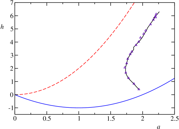
Figure 1: Equilibrium phase diagram of the DNLS model in the $(a,h)$ plane. The positive temperature region lies between the ground state (solid blue line) and the infinite temperature isothermal (dashed red line). The line at constant chemical potential $\mu=2$ has been obtained, for $0.5\leq T\leq 10$, making use of the Monte–Carlo stochastic thermostats [21] (purple triangles) and the Langevin scheme (solid black line).

Finally, above the $T=\infty$ line, one finds the so-called negative-temperature states [18]. In this region, the dynamics of the DNLS equation is characterized by long-lived localized excitations (discrete breathers) [23]. We refer to [24] and to the literature cited therein for a discussion of such peculiar states, whose properties have not yet been fully clarified.

3 Langevin thermostats

The equilibrium properties of the positive-temperature states have been previously explored with the help of Monte–Carlo (MC) thermostats [21], under the assumption of the existence of a grand-canonical statistical measure. As a result, it is for instance possible to reconstruct the states characterized by constant chemical potential (see the triangles in figure 1, which correspond to $\mu=2$).

In this section we present an alternative approach, based on Langevin thermostats [1]. It allows for a more rigorous mathematical formulation and a more direct physical interpretation. In separable Hamiltonian systems (i.e., those composed of a kinetic and a potential energy) interaction with a Langevin bath simply amounts to modify the momentum equation, by adding a linear dissipation term $-\gamma p_{n}$, accompanied by a white-noise fluctuation, whose amplitude determines the temperature value. This simple scheme does not work for the DNLS. In fact, one can easily check that in the limit of vanishing fluctuations (which, supposedly correspond to the zero-temperature limit) this dissipative dynamics converges to a fixed point, that does not correspond to the ground state, which, as mentioned in the previous section, is a time-periodic solution [18].

The problem can be overcome by adopting the following scheme,

$$i\dot{z}_{n}=(1+i\gamma)\left[-2|z_{n}|^{2}z_{n}-z_{n+1}-z_{n-1}\right]+i\gamma\mu z_{n}+\sqrt{\gamma T}\,\xi_{n}(t)\quad,$$ (9)

where $\xi_{n}(t)=\xi^{\prime}_{n}+i\xi^{\prime\prime}_{n}$ is a complex, Gaussian, white random noise with unit variance and $\gamma$ is the coupling strength with the bath. In practice, the above equation, which is basically a stochastic, discrete, complex Ginzburg-Landau equation, corresponds to a series of thermostats all operating at temperature $T$ and chemical potential $\mu$, attached to each lattice site. As required for a meaningful reservoir, the dissipative term vanishes along the ground state evolution, $z_{n}=\sqrt{a}\exp{[i(\omega t+\pi n)]}$.

At variance with MC schemes, one can show (with the help of suitable assumptions and approximations) that eq. (9) describes the coupling with an ensemble of complex linear oscillators (see the derivation in Appendix 1). Additional physical insight is gained by rewriting Eq. (9), in terms of the $p_{n}$, $q_{n}$ variables,

$$\dot{p}_{n} = -\frac{\partial H}{\partial q_{n}}-\gamma\frac{\partial H_{\mu}}{\partial p_{n}}+\sqrt{2\gamma T}\xi_{n}^{\prime}(t)$$ (10)

$$\dot{q}_{n} = \frac{\partial H}{\partial p_{n}}-\gamma\frac{\partial H_{\mu}}{\partial q_{n}}+\sqrt{2\gamma T}\xi_{n}^{\prime\prime}(t)\quad,$$

where and $H_{\mu}$ is the effective Hamiltonian $H_{\mu}=H-\mu A$. In the absence of thermal noise, the deterministic components of the thermostat, being gradient terms, would drive the system towards a state characterized by a minimal $H_{\mu}$. The presence of the symplectic forces allows navigating across the microstates characterized by the given $H_{\mu}$-value. These considerations suggest that this is the proper way to define a dissipation scheme in the DNLS case. Actually, the reason why $H_{\mu}$ is considered instead of $H$ is the presence of two conservation laws: the minimum of the energy depends on the mass density $a$. In order to ensure the convergence to the proper state, the term $-\mu A$ must be added to the effective Hamiltonian. The additional presence of the fluctuations completes the definition of the generalized Langevin equation, which represents a proper stochastic reservoir for the DNLS equation with temperature $T$ and chemical potential $\mu$. From (10) one can also check that the related Fokker-Planck equation admits as a stationary solution the expected equilibrium grandcanonical distribution $\exp\{-\beta(H-\mu A)\}$, with $\beta=1/T$. This setup can be straightforwardly implemented to investigate non–equilibrium settings, by assuming that the single reservoirs operate at different temperatures/chemical potentials.

In the following we will focus on a typical setup adopted in the study of stationary nonequilibrium regimes: only the first ($z_{1}$) and the last ($z_{N}$) lattice variables interact with the reservoirs. This means that, assuming fixed boundary conditions (i.e. $z_{0}=z_{N+1}=0$), the evolution on the leftmost site is ruled by the equation

$$\dot{p}_{1} = -(p_{1}^{2}+q_{1}^{2})q_{1}-q_{2}-\gamma\left[(p_{1}^{2}+q_{1}^{2})p_{1}+p_{2}-\mu_{L}p_{1}\right]+\sqrt{2\gamma T_{L}}\xi^{\prime}_{1}$$ (11)

$$\dot{q}_{1} = (p_{1}^{2}+q_{1}^{2})p_{1}+p_{2}-\gamma\left[(p_{1}^{2}+q_{1}^{2})q_{1}+q_{2}-\mu_{L}q_{1}\right]+\sqrt{2\gamma T_{L}}\xi^{\prime\prime}_{1}\quad,$$

where $T_{L}$ and $\mu_{L}$ denote the temperature and the chemical potential of the left reservoir, respectively. Analogous equations hold for the right reservoir, which acts on the site $n=N$, where the temperature is $T_{R}$, the chemical potential is $\mu_{R}$, and the coupling strength is set again equal to $\gamma$ for simplicity. The rest of the chain follows the Hamiltonian evolution (2).

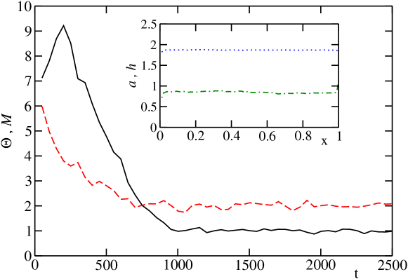
Figure 2: Evolution of $\Theta$ (black solid line) and $\mathcal{M}$ (red dashed line) in a chain of $N=100$ sites in contact with two Langevin heat baths with $T_{L}=T_{R}=1$, $\mu_{L}=\mu_{R}=2$. The initial state corresponds to $a=4$ and $h=15$. $\Theta$ and $\mathcal{M}$ are measured according to [21] and averaged over running windows of 50 time units. In the inset: final spatial profiles of mass (blue dots) and energy (green dot-dashed line) densities as a function of the rescaled site index $x=n/N$.

The simple case of a chain in contact with two reservoirs, operating at the same temperature and chemical potential, allows to test the Langevin scheme (11). In figure 2 we show a typical relaxation process towards an equilibrium state, characterized by the temperature and the chemical potential imposed by the reservoirs. The quantities $\Theta$ and $\mathcal{M}$ on the vertical axis denote the dynamical observables of the DNLS chain representing its microcanonical temperature and chemical potential respectively. Such quantities are complicated functions of the canonical variables, see [8, 21] for details. The inset in figure 2 shows that the asymptotic state reached after the relaxation process is a genuine equilibrium state, corresponding to spatially homogeneous mass and energy densities.

For the sake of completeness, we have also checked the equivalence between the Langevin scheme and the MC reservoirs. As an example, in figure 1 we show that the isochemical lines $\mu=2$, obtained with the two approaches, essentially coincide.

We conclude this section by observing that the scheme (9) reduces, for $T\to\infty$, to a standard Langevin formulation. Actually, in the large temperature limit, but finite mass- and energy-densities, it turns out that $\mu\to-\infty$ and $\gamma\to 0$. In this limit (11) reduces to

$$i\dot{z}_{1}=-2|z_{1}|^{2}z_{1}-z_{2}-i\Gamma z_{1}+\sqrt{a_{L}\Gamma}\,\xi_{1}\ \quad,$$ (12)

where $\Gamma=-\gamma\mu_{L}>0$ and $a_{L}=-T_{L}/\mu_{L}$ are finite quantities. Notice that $a_{L}$, which corresponds to the average mass density in the first site, plays the role of an effective temperature.

As a numerical check, we simulated eq. (12) with $a_{L}>a_{R}$, i.e. in a nonequilibrium setting. Even for relatively short chains, the relation (8) is fulfilled at all points of the chain (see figure 3) meaning that local equilibrium holds. This is further confirmed by the shape of the distribution of the local mass, that is Poissonian, as expected in the $T=\infty$ case [23] (see the inset of figure 3). Establishement of local equilibrium is not granted a priori, although it is known to generically occur in simulations of chains of nonlinear oscillators, even when transport is anomalous [1]. This is nevertheless a peculiar case, as both temperature and chemical potentials are arbitrarily large. However, it should be remarked that local equilibrium relations can be demonstrated to hold exactly only in very simple cases like for instance the Kipnis-Marchioro-Presutti model [25]. For the present model (but also in other nonlinear chains) it is not at all obvious that energy transfer among oscillators can be even roughly approximated by a Markovian process.

Figure 3: Nonequilibrium profiles of mass density (upper panel) and energy density (lower panel) obtained with the infinite temperature Langevin equation (12) and parameters $a_{L}=0.6$, $a_{R}=0.5$, $\Gamma=1$. Black solid, red dashed and blue dot-dashed lines refer respectively to chain lengths $N=25,50,100$. The profiles are almost linear and $h(x)=2a^{2}(x)$ along the chain, confirming that the thermostats act at $T=\infty$. The inset shows that histogram of the local mass $|z_{n}|^{2}$ at $n=20$ is Poissonian, as expected.

4 The low-temperature and large mass density limits

In the previous section we have shown that the Langevin formulation of the DNLS thermodynamics provides a clear physical interpretation of the infinite-temperature limit. In a recent paper [21], it has been found that the opposite, low-temperature, limit, as well as the case of large mass-densities, is also interesting for its nontrivial transport properties. In this section we show that the Langevin formulation can shed further light on such regime by revealing a strong relationship with the XY model and thereby bridging a gap between two seemingly different classes of systems.

It is, first of all, convenient to introduce the following change of variables

$${z}_{n}=\sqrt{a}(1+\zeta_{n})\exp[i(\omega t+\phi_{n}+n\pi)]\quad,$$ (13)

where $\omega=2(a-1)$. By inserting (13) into (2), one finds that the new variables $\zeta_{n}$ and $\phi_{n}$ obey the dynamical equations

$$\dot{\phi_{n}}(1+\zeta_{n}) = 2(1+2a)\zeta_{n}+2a(3\zeta_{n}^{2}+\zeta_{n}^{3})-(1+\zeta_{n+1})\cos(\phi_{n+1}-\phi_{n})$$ (14)

$$-(1+\zeta_{n-1})\cos(\phi_{n}-\phi_{n-1})+2$$

$$\dot{\zeta_{n}} = (1+\zeta_{n+1})\sin(\phi_{n+1}-\phi_{n})-(1+\zeta_{n-1})\sin(\phi_{n}-\phi_{n-1})\quad.$$

In this representation, the ground state (7) is simply $\zeta_{n}=0$, $\phi_{n}=0$. Also, this is the optimal starting point to discuss two limit cases: low-temperatures and large mass-densities. The low-temperature dynamics can be studied by assuming $\zeta_{n}\ll 1$ and ($\phi_{n}-\phi_{n-1})\ll 1$. In Appendix 2, we show that, in this a limit, the system is equivalent to a chain of harmonic oscillators with nearest- and next-to-nearest-neighbour interactions. Furthermore, mass conservation of the original model maps into momentum conservation for the oscillators. Such a correspondence is instructive, as it reveals a link with separable models, where a simple local definition of the temperature can be given in terms of the kinetic energy.

The large mass-density regime is studied under the assumption that $a\gg 1$ and $\zeta_{n}\ll 1$. Here below we show that also in this approximation the Hamiltonian becomes separable. In fact, the dynamical equations (14) reduce to leading order to

$$\dot{\phi_{n}} = \lambda_{n}$$ (15)

$$\dot{\lambda_{n}} = 4a\left[\sin(\phi_{n+1}-\phi_{n})-\sin(\phi_{n}-\phi_{n-1})\right]\quad,$$

where $\lambda_{n}=4a\zeta_{n}$. This system corresponds to a system of coupled rotors, i.e. a classical version of the XY model in one dimension [26, 27, 28, 29]. Its Hamiltonian reads

$$\mathcal{H}_{XY}=\sum_{n}\frac{\lambda_{n}^{2}}{2}-\sum_{n}{4a\cos(\phi_{n+1}-\phi_{n})}\quad,$$ (16)

where $\lambda_{n}$ and $\phi_{n}$ are a couple of conjugate action-angle variables, the former playing the role of the angular momentum. This analogy was already noticed (for the two-dimensional case) in [30].

At variance with the former case, we have not introduced any smallness hypothesis for $\phi_{n}-\phi_{n-1}$; as a result, some nonlinear terms are maintained and one can, thereby, explore large temperatures as well. Having assumed that $\zeta_{n}\ll 1$, this regime can be called phase chaos. It is also interesting to observe that in the large mass–density limit the invariance under global phase rotations of the DNLS transforms into the invariance under a translation of the angles $\phi_{n}$. Accordingly, the conservation of the total mass $A$ transforms into the conservation of the total angular momentum $L=\sum_{n}\lambda_{n}$ (this can be easily verified by expanding expression (5)). Notice also that the low-temperature limit discussed in Appendix 2 is not fully contained into the large mass-density regime, as it includes the case of relatively small $a$-values.

Before passing to thermodynamic studies, it is necessary to clarify the range of validity of the XY model as an approximation of the DNLS one. The condition $\zeta_{n}\ll 1$ implies $\lambda_{n}\ll a$, i.e. $T\ll a^{2}$, because on average $\lambda_{n}^{2}$ is equal to the temperature $T$. As we are exploring the range of large $a$-values, one can conclude that, the larger $a$, the broader the temperature range where the XY model provides an accurate description of the DNLS equation. Before drawing this conclusion, it is, however, necessary to be more careful. In fact, the presence of a finite conductivity in the XY model can be traced back to the existence of (possibly infrequent) jumps of angle-differences across the sinusoidal potential barrier. In the context of Eq. (16), the height of this barrier is of the order of $a$, which is smaller than the maximal acceptable energy $a^{2}$ (since $a\ll a^{2}$, for $a\gg 1$). Accordingly the XY model provides an accurate description also of the barrier jumps and, more than that, the validity of the XY model extends to the high-temperature regime (here “high” means above $a$) characterized by frequent jumps.

4.1 Thermostatted chain

Here, we examine how to describe the bath dynamics within the XY approximation. Let us study the simple setup of a DNLS chain in contact with an external Langevin reservoir at the first site. In the low-temperature limit, i.e. close to the ground state, equation (9) specializes to

$$i\dot{z}_{1}=-2|z_{1}|^{2}z_{1}-z_{2}-i\gamma\left[2|z_{1}|^{2}z_{1}+z_{2}-2(a-1)z_{1}-\delta\mu\,z_{1}\right]+\sqrt{\gamma T_{L}}\,\xi_{1}\,.$$ (17)

We have consistently assumed the chemical potential to be a perturbation of the ground-state value, i.e. $\mu=\omega+\delta\mu$ with $\delta\mu\ll\omega$. For $a\gg 1$, (17) transforms, to leading order in $a$, into a Langevin equation for the XY model with suitable dissipation and fluctuation terms

$$\dot{\phi_{1}} = 4a\zeta_{1}$$ (18)

$$\dot{\zeta_{1}} = \sin(\phi_{2}-\phi_{1})-\gamma\left(4a\zeta_{1}-\delta\mu\right)+\sqrt{\frac{\gamma T_{L}}{a}}\,\xi_{1}\quad.$$

By then introducing the momenta $\lambda_{n}$, equation (15), and the rescaled dissipation parameter $\gamma^{\prime}=4a\gamma$, one finally obtains

$$\dot{\phi_{1}} = \lambda_{1}$$ (19)

$$\dot{\lambda_{1}} = 4a\sin(\phi_{2}-\phi_{1})-\gamma^{\prime}\left(\lambda_{1}-\delta\mu\right)+\sqrt{4\gamma^{\prime}T_{L}}\,\xi_{1}\quad.$$

These equations describe a rotor chain in contact in the first site with a reservoir at temperature $2T_{L}$ and constant torque $\gamma^{\prime}\delta\mu$.

This derivation provides an interesting interpretation of the DNLS chemical potential in the large mass-density limit: at equilibrium (19) is expected to sample microstates compatible with the grandcanonical measure $\exp{\{-\beta[\mathcal{H}_{XY}-\delta\mu L]\}}$, where $L=\sum_{n}\lambda_{n}$ is the total angular momentum of the XY chain and $\delta\mu$ can be interpreted as the average angular velocity of the rotors.

4.2 Nonequilibrium conditions

The above formulation can be straightforwardly extended to nonequilibrium setups, where $T_{R}\neq T_{L}$ and $\mu_{R}\neq\mu_{L}$. In this case, it is convenient to perform the XY approximation with respect to a ground state that corresponds to the average chemical potential $(\mu_{R}+\mu_{L})/2$. Accordingly, the resulting XY chain turns out to be forced by opposite external torques $\pm\gamma^{\prime}\delta\mu$, where now $\delta\mu=(\mu_{R}-\mu_{L})/2$.

The observables of major interest in the nonequilibrium context are the fluxes of the conserved quantities. The continuity equations for mass and energy densities of the DNLS model allow determining their explicit expressions

$$j_{n}^{a} = i(z_{n}z_{n-1}^{*}-z_{n}^{*}z_{n-1})$$ (20)

$$j_{n}^{h} = \dot{z}_{n}z_{n-1}^{*}+\dot{z}_{n}^{*}z_{n-1}\quad.$$ (21)

In the large mass-density limit, the leading terms read

$$j_{n}^{a} = -2a\sin(\phi_{n+1}-\phi_{n})$$ (22)

$$j_{n}^{h} = -2\omega\,a\sin(\phi_{n+1}-\phi_{n})-4a\dot{\phi}_{n}\sin(\phi_{n+1}-\phi_{n})\quad,$$ (23)

where the variables $\zeta_{n}$ have been expressed in terms of $\dot{\phi}_{n}$. Notice that the simple symmetric form of the second equation has been obtained by adding to (21) the quantity $-a(\dot{\phi}_{n}-\dot{\phi}_{n-1})\sin(\phi_{n}-\phi_{n-1})$, whose average is zero in a stationary state. Eq. (22) is just the momentum flux of the XY model, i.e. the local force. The term proportional to $\dot{\phi}_{n}$ in Eq. (23) has the typical structure of the energy flux in the XY model: it is nonzero only at finite temperatures. The first term is a coherent contribution that results from the fact that the oscillators rotate with an average common frequency $\omega$: it survives in the zero-temperature limit, when $j^{h}_{n}=\mu j^{a}_{n}$, so that the heat current $j^{h}_{n}-\mu j^{a}_{n}=0$, i.e. there is no heat transport and no entropy production. At low temperatures, Eqs. (22,23) describe the Josephson effect, where the chain amounts to a single junction in between two superfluids [31]. The mass current is proportional to the phase gradient and is independent of the system length $N$, i.e. it provides a ballistic contribution.

5 Comparison with numerical simulations

As mentioned above, an important difference between the DNLS equation and oscillator chains (like the Fermi-Pasta-Ulam or Klein-Gordon models) is that its Hamiltonian is not the sum of kinetic and potential energies. Therefore, it is not obvious how to directly monitor the temperature $T$ and the chemical potential $\mu$ in actual simulations. The only general approach we are aware of is based on non-local microcanonical expressions $\Theta$ and $\mathcal{M}$ [32] which, unfortunately are rather awkward to compute in practice (see [21] for details). The perturbative analysis of the low-temperature limit and the correspondence with the XY model show that the temperature $T$ and the chemical potential $\mu$ can be determined in terms of local variables. This is quite a relevant observation as it may be used to simplify the definition of such thermodynamic quantities. In the following we explore the range of validity of such definitions.

From (16) it is straightforward to define a kinetic temperature as the fluctuations of the momentum $\lambda_{n}$ with respect to its average value $\langle\lambda_{n}\rangle$,

$$T_{XY}=\langle\lambda_{n}^{2}\rangle-\langle\lambda_{n}\rangle^{2}\quad.$$ (24)

If we compare the stochastic term in (19) with the one imposed by the fluctuation-dissipation theorem and commonly used in the Langevin equation for oscillator models, $\sqrt{2\gamma T}$ (see [1, 2]), we can conclude that our definitions imply $T_{XY}=2T$ (the factor 2 is just a consequence of the choice of the transformation of variables).

In figure 4 we compare the general microcanonical definition of temperature for the DNLS model $\Theta$, defined as in [21], with $T_{XY}$ for an equilibrium setting, i.e. external reservoirs at equal temperature and chemical potential; $T_{XY}$ is computed by evaluating, in the same simulation, the average of the $\zeta_{n}^{2}$ defined in (13). The data clearly show that, by increasing the chemical potential $\mu$ (i.e., by increasing $a$, since $\mu=2(a-1)$), the range of values in which the two temperatures coincide increases, as expected from the previous considerations. On the other hand, outside the limits of validity of the XY approximation discussed in section 4, $\Theta$ and $T_{XY}$ can be strongly different from one another. In such regimes, $\Theta$ is the only valid definition of temperature. In the inset of figure 4 we show that the curves obtained for different values of $\mu$ quite well collapse onto each other by rescaling both $T_{XY}$ and $\Theta$ by the factor $a^{-2}$. This implies that the range of validity of the correspondence between these two temperatures increases proportionally to $a^{2}$.

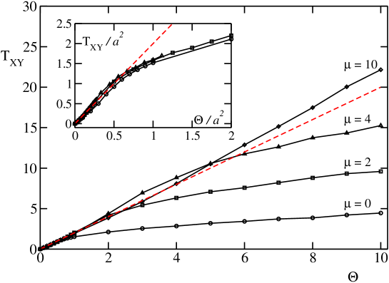
Figure 4: Comparison of the XY kinetic temperature $T_{XY}$ with $\Theta$ for different values of the chemical potential $\mu$. The dashed line corresponds to $T_{XY}=2\Theta$, which should hold in the limit of large $\mu$, where the XY approximation is valid. The inset shows the same curves in the rescaled units $T_{XY}/a^{2}$ and $\Theta/a^{2}$. Simulations are performed using Langevin heat baths coupled at the boundaries of a DNLS chain with $N=50$. $T_{XY}$ and $\Theta$ are measured on a subchain of $30$ lattice sites.

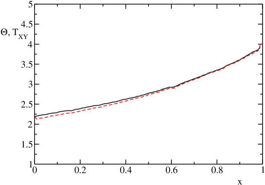
Figure 5: Comparison of the XY kinetic temperature profile $T_{XY}$ (red dashed line) with $\Theta$ [21] (black solid line) in a nonequilibrium steady state. Simulations are performed using Langevin heat baths with parameters ($T_{L}=2$, $\mu_{L}=9.6$) and ($T_{R}=4$, $\mu_{R}=10.4$), coupled to a DNLS chain with $N=1000$.

Finally, we have tested the validity of the XY approximation in a non-equilibrium stationary regime. In the simplest case one can impose two heat baths at different temperatures, $T_{R}$ and $T_{L}$, and with the same chemical potential $\mu$ acting at the chain boundaries. If one chooses the value of $\mu$ in such a way that both temperatures are smaller than $a^{2}$ (see figure 4), one obtains temperature profiles very close to each other (data not reported). This scenario is maintained also if a chemical potential gradient is applied, provided both $\mu_{R}$ and $\mu_{L}$ are large enough to make the previous condition hold, while $\delta\mu=(\mu_{R}-\mu_{L})/2$ is smaller than the average chemical potential $(\mu_{R}+\mu_{L})/2$ (see sections 4.1 and 4.2 ). In fact, figure 5 exhibits a nice agreement between the two temperature profiles. A further test of the validity of XY model is presented in Table 1 where the full DNLS fluxes are compared with the ones reconstructed through the XY approximation (see Eqs. (22) and (23)  ).

	DNLS	XY
$j^{a}$	-0.234	-0.208
$j^{h}$	-1.40	-1.28

Table 1: Comparison of the exact DNLS fluxes (first column) and the ones reconstructed by means of eqs.(22) (second column) for the nonequilibrium profile described in the caption of figure 5.

6 Conclusions

In this paper we have introduced Langevin heat baths which are able to control both the temperature and the chemical potential in a DNLS model. Numerical simulations indicate that such scheme is simple and practical enough to study finite-temperature DNLS dynamics in both equilibrium and nonequilibrium conditions.

In the low-temperature and large mass-density limit we have approximated the DNLS dynamics in terms of an effective XY model. This allows a clear understanding of the DNLS dynamics, especially in a nonequilibrium setting. We have indeed shown that the effect of thermal baths (which are able to control the chemical potential besides the temperature) acting at the boundaries, is equivalent to an applied torque plus thermal fluctuations. This description allows to give a dynamical interpretation of the chemical potential as well as of the action of thermal baths as means to fix locally the average angular velocities. The corresponding energy flux turns out to be the sum of two different contributions, one due to the phase gradient associated with the torque, the other due to angular-velocity fluctuations. As a consequence, transport in this region has an almost ballistic component, and a diffusive one associated with the XY dynamics which is known to be a normal heat conductor [26, 27]. This accounts for several previous computations of transport coefficients [21].

Another remarkable result, is that the relationship with the XY model provides a simple prescription for computing the temperature in the simulations. This last issue is of major importance for non-standard Hamiltonians like the DNLS one, where kinetic and potential energies are not separated. Indeed, the XY approximation allows introducing the simple kinetic expression $T_{XY}$ for the temperature, that can safely approximate the microcanonical one $\Theta$. This is of practical importance, considering that the microscopic definitions of $T$ and $\mu$ are pretty much involved for a non separable Hamiltonian, like the DNLS one [32].

Altogether, starting from the Langevin approach we have achieved a fairly clear physical interpretation of the action of thermal baths as means to fix locally the average angular velocities and kinetic energies of the oscillators. In the framework of the nonequilibrium XY model this means that one can explore more general nonequilibrium states by applying not only temperature but also mechanical (torque) gradients. This possibility has not received much attention in the literature. To our knowledge, only reference [33] treats the joint effect of thermal and mechanical gradients (see also the nonequilibrium studies in [34] that however refer to the case without external torque and noise).

Some of the numerical results presented above are possible starting points for rigorous investigations. For instance, the evidence of local equilibrium reported in section 3 and the possible approximate description in terms of stochastic models [25] could be a challenging issue for mathematical studies.

Another possible extension of the present work would be to consider the DNLS model on two-dimensional lattices. In this case, the correspondence with the XY model would predict the possibility of observing the transition from normal to anomalous behavior of transport coefficients at the Kosterlitz-Thouless-Berezhinskii transition [35, 36].

Appendix 1: Derivation of the Langevin equation

In this appendix we derive Eq. (9) by following the system-bath coupling approach [37]. In analogy with what done for harmonic lattices [38], we consider a complex oscillator, described by the dynamical variable $z$, linearly coupled with a bath of independent, complex harmonic oscillators described by the Hamiltonian

$$H_{B}=\sum_{\nu}\{\omega_{\nu}^{a}|a_{\nu}|^{2}+\omega_{\nu}^{b}|b_{\nu}|^{2}+\left[K_{\nu}^{*}z(a_{\nu}^{*}+b_{\nu})+c.c.\right]\}\quad,$$ (25)

where we have introduced two different species of oscillators, corresponding to the two sets of frequencies $\omega_{\nu}^{a}$ and $\omega_{\nu}^{b}$, while $K_{\nu}$ are the bath-system coupling constants. Moreover, the variables $(a_{\nu},ia^{*}_{\nu})$ and $(b_{\nu},ib^{*}_{\nu})$ are independent canonically conjugate coordinates, satisfying the following Poisson brackets

$$\{ia_{\nu}^{*},a_{\nu^{\prime}}\}=\{ib_{\nu}^{*},b_{\nu^{\prime}}\}=\delta_{\nu,\nu^{\prime}}$$ (26)

$$\{a_{\nu},a_{\nu^{\prime}}\}=\{b_{\nu},b_{\nu^{\prime}}\}=\{a_{\nu},b_{\nu^{\prime}}\}=\{a_{\nu},ib_{\nu^{\prime}}^{*}\}=0\quad.$$

In order to preserve the global symmetry of the system with respect to phase transformations, we impose a second conservation law,

$$A_{B}=\sum_{\nu}(|a_{\nu}|^{2}-|b_{\nu}|^{2})\quad.$$ (27)

The function $A_{B}$ is the generator of phase transformations of the bath variables. It is easy to verify that the transformation generated by $A_{B}+|z|^{2}$,

$$a_{\nu}(s) = e^{is}a_{\nu}(0)$$

$$b_{\nu}(s) = e^{-is}b_{\nu}(0)$$

$$z(s) = e^{is}z(0)\quad,$$

leaves the Hamiltonian $H_{B}$ invariant. An example of heat bath satisfying these conditions is given by a complex d’Alembert equation, $\Box\phi(x,t)=0$, for which the quantity $A_{B}$ represents the total (conserved) charge of the field. The equations of motion generated by (25) are

$$i\dot{a}_{\nu}=-\omega_{\nu}^{a}\,a_{\nu}-K_{\nu}^{*}z$$

$$i\dot{b}_{\nu}=-\omega_{\nu}^{b}\,b_{\nu}-K_{\nu}z^{*}$$

$$i\dot{z}=f(z)-\sum_{\nu}K_{\nu}(a_{\nu}+b_{\nu}^{*})\quad,$$

where $f(z)$ accounts for the deterministic part of the evolution of $z$, not included in $H_{B}$. The first two equations can be formally solved, yielding

$$a_{\nu}(t)=a_{\nu}(0)\,e^{i\omega_{\nu}^{a}t}+iK_{\nu}^{*}\int_{0}^{t}\,e^{i\omega_{\nu}^{a}(t-t^{\prime})}z(t^{\prime})\,dt^{\prime}$$

$$b_{\nu}(t)=b_{\nu}(0)\,e^{i\omega_{\nu}^{b}t}+iK_{\nu}\int_{0}^{t}\,e^{i\omega_{\nu}^{b}(t-t^{\prime})}z^{*}(t^{\prime})\,dt^{\prime}\,.$$

By then substituting into the equation for $z$, we obtain

$$i\dot{z}=f(z)-i\int_{0}^{t}G(t-s)z(s)ds+F(t)\quad,$$

where the noise term $F(t)$ and the dissipation function $G(t)$ are defined as

$$F(t)=-\sum_{\nu}K_{\nu}\left[a_{\nu}(0)e\,^{i\omega_{\nu}^{a}t}+b_{\nu}^{*}(0)\,e^{-i\omega_{\nu}^{b}t}\right]$$ (28)

$$G(t)=\sum_{\nu}|K_{\nu}|^{2}\left[e^{i\omega_{\nu}^{a}t}-e^{-i\omega_{\nu}^{b}t}\right]\quad.$$ (29)

By now imposing a grandcanonical equilibrium distribution $P\sim\exp[-\beta(H_{B}-\mu A_{B})]$ for the bath of oscillators (where $\beta=1/T$ is the inverse temperature) [23], we find that the correlation functions of $F(t)$ read

$$\langle F(t)F(t^{\prime})\rangle = \langle F^{*}(t)F^{*}(t^{\prime})\rangle=0$$

$$\langle F(t)F^{*}(t^{\prime})\rangle = \sum_{\nu}|K_{\nu}|^{2}\left[e^{i\omega_{\nu}^{a}(t-t^{\prime})}\,\langle\,|a_{\nu}(0)|^{2}\,\rangle+e^{-i\omega_{\nu}^{b}(t-t^{\prime})}\,\langle\,|b_{\nu}(0)|^{2}\,\rangle\right]=$$ (30)

$$\sum_{\nu}|K_{\nu}|^{2}\left[\frac{e^{i\omega_{\nu}^{a}(t-t^{\prime})}}{\beta(\omega_{\nu}^{a}-\mu)}+\frac{e^{-i\omega_{\nu}^{b}(t-t^{\prime})}}{\beta(\omega_{\nu}^{b}+\mu)}\right]\,,$$

where, in order to have positive definite statistical weights, we have also to assume $\omega_{\nu}^{a}>\mu$ and $\omega_{\nu}^{b}>-\mu$. In the thermodynamic limit the sums over the index $\nu$ in (29) can be replaced by integrals. Accordingly, we can rewrite Eq. (29) in the form

$$G(t)=\int_{\mu}^{+\infty}\,d\omega\,G^{a}(\omega)\,e^{i\omega t}-\int_{-\mu}^{+\infty}\,d\omega\,G^{b}(\omega)\,e^{-i\omega t}\quad,$$ (31)

where $G^{a,b}(\omega)=\rho^{a,b}(\omega)|K(\omega)|^{2}$ are two positive definite functions and $\rho^{a,b}(\omega)$ the corresponding density of states that we assume to be smooth functions. By following the same approach, Eq. (30) writes

$$\langle F(t)F^{*}(t^{\prime})\rangle=\int_{\mu}^{+\infty}d\omega\,\frac{G^{a}(\omega)e^{i\omega(t-t^{\prime})}}{\beta(\omega-\mu)}+\int_{-\mu}^{+\infty}d\omega\,\frac{G^{b}(\omega)e^{-i\omega(t-t^{\prime})}}{\beta(\omega+\mu)}\quad,$$ (32)

which is a kind of fluctuation-dissipation theorem [38] where the Bose-Einstein distribution has been replaced by the Rayleigh-Jeans one.

The corresponding generalized Langevin equation is not very practical, since it is non Markovian. We have nevertheless the freedom to choose the coupling and the density of states of the bath. The spectral properties of the process $F$ strongly depend on the behaviour of $G$ close to the ground state and may also display long-range correlations. To understand this point, consider the example in which $G^{a,b}(\omega)=\gamma$. This choice yields a spectral density of $F(t)$ which is logarithmically divergent close to the ground state frequency, thus defining a non-stationary process. The simplest, nonsingular case is obtained by choosing

$$G^{a}(\omega)=\frac{\gamma}{2\pi}(\omega-\mu),\quad G^{b}(\omega)=\frac{\gamma}{2\pi}(\omega+\mu)\quad.$$

In this case $F(t)$ becomes a complex white noise

$$\langle F(t)F^{*}(t^{\prime})\rangle=\frac{\gamma}{\beta}\delta(t-t^{\prime})\quad,$$

while the dissipation function is

$$G(t)=\frac{\gamma}{2\pi}\int_{-\infty}^{+\infty}d\omega\,(\omega-\mu)e^{i\omega t}=-\gamma\left[i\frac{d}{dt}\delta(t)+\mu\delta(t)\right]\quad.$$ (33)

The full dissipation term is therefore

$$-i\int_{0}^{t}G(t-s)z(s)\,ds=-\gamma\dot{z}(t)+i\gamma\mu z(t)\quad,$$ (34)

and the resulting Langevin equation corresponds to a noisy, driven, complex Ginzburg-Landau equation

$$(i+\gamma)\dot{z}=f(z)+i\gamma\mu z+F(t)\quad.$$ (35)

In the weak coupling limit ($\gamma\ll 1)$, the equation can be further simplified. By multiplying by $(1+i\gamma)$ and neglecting terms $O(\gamma^{3/2})$, one obtains

$$i\dot{z}=(1+i\gamma)f(z)+i\gamma\mu z+F(t)\quad,$$ (36)

which has the same structure as Eq. (9).

Appendix 2: The low–temperature limit of the DNLS problem

In this appendix we provide a low–temperature description of the DNLS equation in terms of a harmonic model with separable Hamiltonian. In this limit, the solution of Eq. (14) is expected to be close to the homogeneous periodic motion of the ground-state solution (7). Thus, we assume $\zeta_{n}\ll 1$ and $(\phi_{n}-\phi_{n-1})\ll 1$ and we expand Eq. (14) to linear order. As a result, we obtain

$$\dot{\phi}_{n} = 4a\zeta_{n}+2\zeta_{n}-\zeta_{n+1}-\zeta_{n-1}$$ (37)

$$\dot{\zeta}_{n} = \phi_{n+1}-2\phi_{n}+\phi_{n-1}\quad.$$

If one now introduces the new variable

$$p_{n}=4a\zeta_{n}+2\zeta_{n}-\zeta_{n+1}-\zeta_{n-1}\quad.$$ (38)

the Eqs. (37) can be re–written as

$$\dot{\phi}_{n} = p_{n}$$ (39)

$$\dot{p}_{n} = 4(1+a)(\phi_{n+1}-2\phi_{n}+\phi_{n-1})-\phi_{n+2}+2\phi_{n}-\phi_{n-2}\quad.$$

These equations describe the dynamics of a chain of harmonic oscillators with nearest-neighbour and next-to-nearest-neighbour interaction. The corresponding Hamiltonian,

$$\mathcal{H}_{h}=\sum_{n}\left[\frac{1}{2}p_{n}^{2}+2(1+a)(\phi_{n+1}-\phi_{n})^{2}-\frac{1}{2}(\phi_{n+2}-\phi_{n})^{2}\right]\quad,$$ (40)

is, at leading order in $p_{i}$ and $(\phi_{n+1}-\phi_{n})$, fully equivalent to that of the original DNLS equation. Its quadratic structure corresponds to a parabolic approximation around the minimum of the energy. Moreover, the total mass-conservation law of the DNLS maps onto the conservation of the total momentum $P=\sum p_{n}$. Accordingly, the Hamiltonian (40) is translationally invariant. The normal modes, i.e. the plane-wave solutions of Eqs. (39), are the discrete analogs of the Bogoliubov modes (non-interacting phonons), in the context of the physics of atomic condensates [31].

Passing to thermodynamics, one interesting implication of the Hamiltonian structure in the low–temperature limit (40) is that one can naturally introduce a microscopic definition of temperature in terms of the momentum $p_{n}$, i.e.

$$T_{h}=J\left[\langle p_{n}^{2}\rangle-\langle p_{n}\rangle^{2}\right]$$ (41)

where the proportionality constant $J$ is the Jacobian determinant of transformation (38), which must be included to allow for a meaningful comparison with the DNLS model. In order to test the definition (41), we have measured $T_{h}$ by numerical simulations of the Langevin scheme defined in Eq. (9) and in figure 6 we have compared it with the temperature of the bath, $T_{B}\equiv T_{L}=T_{R}$, for different values of the mass density, $a$. As expected, $T_{h}$ approaches $T_{B}$ for increasing values of $a$. In fact, the larger is $a$, the smaller is the relative amplitude of the fluctuations with respect to the ground state. From this analysis we therefore conclude that the harmonic temperature $T_{h}$ is a well defined thermodynamic observable in the low–temperature limit. Such a definition is much simpler than the general microcanonical one, $\Theta$, defined in [21, 32].

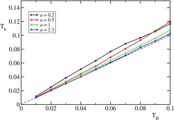
Figure 6: Comparison of the harmonic temperature $T_{h}$, Eq. (41) with the reservoir temperature, $T_{B}$. The dashed line correspond to $T_{h}=T_{B}$. The Langevin heat baths are coupled at the boundaries of a DNLS chain with $N=50$. $T_{h}$ is measured on a subchain of $30$ lattice sites to increase the statistics. The values of the Jacobian determinant $J$, which are the product of the eigenvalues of a tridiagonal matrix, have been computed analytically in the $N\to\infty$ limit and are $J=5.95,3.73,2.91,2.42$ for curves from top to bottom.

For what concerns transport properties, the heat conductivity of the harmonic model (40) exhibits a divergence in the thermodynamic limit, as expected for any integrable model (see [39, 1]). Such a conclusion is in contrast with previous non-equilibrium numerical studies of the DNLS model [21] that have revealed a finite heat conductivity at finite temperatures. This is clearly a consequence of the presence of nonlinear terms which break the integrability of the dynamics. Their contribution is taken into account in section 4, where we discuss the tight relationship with the one-dimensional XY model in the limit of large mass densities. In this respect, it is useful to compare the harmonic hamiltonian $H_{h}$ (40) with the one corresponding to the XY model (16). The former is valid in the low-temperature regime, while the latter applies for $a\gg 1$ (and $T\ll a^{2}$). Accordingly, they reduce to one another for small $T$ and large $a$. In this limit, in fact, the next–to–nearest-neighbour interaction in (40) is negligible for $a\gg 1$ and, in the low–temperature limit, one can expand the cosine interaction in (16) around zero.

References

References

- [1] Lepri S, Livi R and Politi A 2003 Phys. Rep. 377 1
- [2] Dhar A 2008 Adv. Phys. 57 457–537
- [3] Eilbeck J C, Lomdahl P S and Scott A C 1985 Physica D 16 318–338
- [4] Kevrekidis P G 2009 The Discrete Nonlinear Schrödinger Equation (Springer Verlag, Berlin)
- [5] Scott A 2003 Nonlinear science. Emergence and dynamics of coherent structures. (Oxford University Press, Oxford)
- [6] Kosevich A M and Mamalui M A 2002 J. Exp. Theor. Phys. 95 777
- [7] Hennig D and Tsironis G 1999 Phys. Rep. 307 333–432
- [8] Franzosi R, Livi R, Oppo G and Politi A 2011 Nonlinearity 24 R89
- [9] Delfini L, Lepri S, Livi R and Politi A 2007 J. Stat. Mech.: Theory and Experiment P02007
- [10] Basile G, Bernardin C and Olla S 2006 Phys. Rev. Lett. 96 204303
- [11] Gillan M and Holloway R 1985 J. Phys. C 18 5705–5720
- [12] Mejía-Monasterio C, Larralde H and Leyvraz F 2001 Phys. Rev. Lett. 86 5417–5420
- [13] Larralde H, Leyvraz F and Mejía-Monasterio C 2003 J. Stat. Phys. 113(1) 197–231
- [14] Casati G, Wang L and Prosen T 2009 J. Stat. Mech.: Theory and Experiment L03004
- [15] Saito K, Benenti G and Casati G 2010 Chem. Phys. 375 508–513
- [16] Flach S and Gorbach A V 2008 Physics Reports 467 1–116
- [17] Lebowitz J, Rose H and Speer E 1988 J. Stat. Phys. 50 657–687
- [18] Rasmussen K, Cretegny T, Kevrekidis P G and Grønbech-Jensen N 2000 Phys. Rev. Lett. 84 3740–3743
- [19] Johansson M 2006 Physica D 216 62–70
- [20] Basko D 2011 Annals of Physics 326 1577 – 1655
- [21] Iubini S, Lepri S and Politi A 2012 Phys. Rev. E 86 011108
- [22] Christiansen P L, Gaididei Y B, Johansson M and Rasmussen K O 1997 Phys. Rev. B 55 5759–5766
- [23] Rumpf B 2004 Phys. Rev. E 69 016618
- [24] Iubini S, Franzosi R, Livi R, Oppo G and Politi A 2013 New J. Phys. 15 023032
- [25] Kipnis C, Marchioro C and Presutti E 1982 J. Stat. Phys. 27 65
- [26] Giardiná C, Livi R, Politi A and Vassalli M 2000 Phys. Rev. Lett. 84 2144–2147 ISSN 0031-9007
- [27] Gendelman O V and Savin A V 2000 Phys. Rev. Lett. 84 2381–2384
- [28] Yang L and Hu B 2005 Phys. Rev. Lett. 94(21) 219404
- [29] Escande D, Kantz H, Livi R and Ruffo S 1994 J. Stat. Phys. 76 605–626
- [30] Trombettoni A, Smerzi A and Sodano P 2005 New Journal of Physics 7 57
- [31] Smerzi A, Trombettoni A, Kevrekidis P G and Bishop A R 2002 Phys. Rev. Lett. 89(17) 170402
- [32] Franzosi R 2011 J. Stat. Phys. 143(4) 824–830
- [33] Iacobucci A, Legoll F, Olla S and Stoltz G 2011 Phys. Rev. E 84 061108
- [34] Eleftheriou M, Lepri S, Livi R and Piazza F 2005 Physica D: Nonlinear Phenomena 204 230–239
- [35] Leoncini X, Verga A D and Ruffo S 1998 Phys. Rev. E 57 6377
- [36] Delfini L, Lepri S and Livi R 2005 J. Stat. Mech: Theory Exp. P05006
- [37] Zwanzig R 2001 Nonequilibrium Statistical Mechanics (Oxford University Press, USA)
- [38] Dhar A and Roy D 2006 J. Stat. Phys. 125 805
- [39] Rieder Z, Lebowitz J L and Lieb E 1967 J. Math. Phys. 8 1073