Out-of-equilibrium one-dimensional disordered dipole chain

Abstract

We consider a chain of one-dimensional dipole moments connected to two thermal baths with different temperatures. The system is in nonequilibrium steady state and heat flows through it. Assuming that fluctuation of the dipole moment is a small parameter, we develop an analytically solvable model for the problem. The effect of disorder is introduced by randomizing the positions of the dipole moments. We show that the disorder leads to Anderson-like transition from conducting to a thermal insulating state of the chain. It is shown that considered chain supports both ballistic and diffusive heat transports depending on the strength of the disorder. We demonstrate that nonequilibrium leads to the emergence of the long-range order between dipoles along the chain and make the conjecture that the interplay between nonequilibrium and next-to-nearest-neighbor interactions results in the emergence of long-range correlations in low-dimensional classical systems.

I Introduction

The understanding of out-of-equilibrium low-dimensional systems has been a challenging problem for decades. This topic covers a large variety of important problems of modern physics concerning, for example, the necessary conditions for the observation of the Fourier law Bonetto et al. (2000); Dubi and Di Ventra (2009); Dubi and Di Ventra (2009, 2011); how to achieve and manipulate directed transport in systems with Brownian motion Reimann (2002); Hänggi (2009); how to gain a useful work in nonequilibrium Reimann (2002); Gelin and Kosov (2008); how to control the energy transport in one- and two-dimensional assemblies of large organic molecules with high dipole moment arranged on a surface Kottas et al. (2005); de Jonge et al. (2007); Horansky et al. (2006); the mechanism of the transition to chaos in nonlinear chains Ford (1992); the necessary conditions for the occurrence and existence of the temporally periodic and spatially localized excitations in nonlinear chains Aubry (2006); the unique steady state’s existence in nonlinear chains Eckmann et al. (1999). Nonequilibrium processes in low-dimensional systems are also of practical and technological interest because of the recent advances in nanofabrication.

In this paper, we consider an out-of-equilibrium one-dimensional chain of particles interacting with each other via the classical dipolar potential. Our interest is twofold. First, we consider a heat conduction in such chains. Second, we study the emergence of new correlations in the system caused by a heat flow.

We approximate a particle by a point dipole placed at a fixed position on a line. This approximation is valid for different real physical systems. For instance, molecules of artificial molecular rotors contain one or several chemical groups with substantial dipole moment. While the rest of the molecule is kept fixed on a surface these groups rotate Kottas et al. (2005); Horansky et al. (2006). The dipole chain model is also intimately connected with ferrofluids or solid-state magnetic dipoles Shelton (2005); Murashov et al. (2002); Klapp (2005). The point dipole approximation is valid for a single-file water chain Hummer et al. (2001); Köfinger et al. (2008). The water in narrow single wall carbon nanotubes forms a strongly ordered one-dimensional chain Hummer et al. (2001); Kyakuno et al. (2011). Each water molecule is connected by two hydrogen bonds to neighbor molecules, instead of four bonds in bulk, and also interacts with the carbon atoms of the nanotube. The latter interaction is weak compared to the dipolar one, but owing to the high density of the carbon atoms, it is not negligible and leads to the additional stabilization of the water in nanotube Alexiadis and Kassinos (2008); Köfinger et al. (2011). The hydrogen bonds in 1D water are energetically stronger and possess longer life-time than ones in a bulk Hummer et al. (2001). Both of these facts lead to the formation of the stable water molecules chain in narrow carbon nanotubes or pores Hummer et al. (2001); Köfinger et al. (2009). Moreover, equations of motion of dipole chain can be treated as a particular case of Kuramoto model Kuramoto (1984); Acebrón et al. (2005). In its turn, this model describes in a broad sense the synchronization in dynamical system of coupled oscillators. It is clear that this formulation is related to a number of phenomena from synchronization of cells in human organism to phase transitions or Brownian motors. The systems with dipole-dipole interaction occur not only in a classical physics, but also play an important role in quantum world. For instance, in a rapidly growing area of cold dipolar atomic gases Lahaye et al. (2009); Arkhipov et al. (2005). For example, in the high density limit single-file quantum dipoles can also form a lattice with a strong localization of atoms near lattice sites Arkhipov et al. (2005).

The remainder of the paper is organized as follows. In Sec. II, we describe the Langevin nonequilibrium dynamics for the one-dimensional chain of dipoles, theoretical approach to treat the disordered and the method to compute nonequilibrium correlation functions. Section III presents the results of the numerical calculations. Conclusions are given in Sec. IV. Some technical aspects are relegated to appendices.

II Mathematical formalism

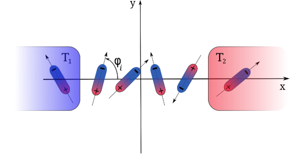
Figure 1: The sketch of the 1D dipole chain. Dipoles are represented by vectors with appropriate magnitude and orientation. In polar coordinates the state of the dipole is described by its magnitude and polar angle $\displaystyle\varphi$. There are two heat baths that support a heat flow along a chain. The left bath is the ”cold” one, i.e., $\displaystyle T_{L}<T_{R}$.

II.1 Nonequilibrium dynamics

Let us consider a 1D chain of the $\displaystyle N$ point dipoles with magnitude $\displaystyle\mu$. The dipoles are rendered on a single line with a distance $\displaystyle a$ between them and are supposed to rotate in plane $\displaystyle(x,y)$ around the axes perpendicular to the plane of the dipole. The position of the arbitrary dipole is characterized by a single angle $\displaystyle\varphi$, Fig. 1. Thus, our model is purely one-dimensional. The classical Hamiltonian of the dipole chain has the form:

$$\displaystyle H=K+U=\frac{I}{2}\sum\limits_{i=1}^{N}\dot{\varphi}_{i}^{2}+\frac{\mu^{2}}{a^{3}}\sum\limits_{i=1}^{N}\sum\limits_{j=i+1}^{i+N_{cut}-1}\left(\frac{\sin{\varphi_{i}}\sin{\varphi_{j}-2\cos\varphi_{i}\cos\varphi_{j}}}{|r_{i}-r_{j}|^{3}}\right),$$ (II.1)

where $\displaystyle I$ is the moment of inertia of the dipole, $\displaystyle\varphi_{i}$ is the angle between the vector of dipole moment of the $\displaystyle i$th dipole and the axis $\displaystyle x$, $\displaystyle r_{i}$ is the dimensionless position (in units of $\displaystyle a$) of the $\displaystyle i$th dipole moment and dot stands for time derivative, $\displaystyle N_{cut}=2,3,\ldots,N$ defines an interaction range and in what follows we call it cutoff radius.

The left and right dipoles of the chain are coupled by some mechanism to two macroscopic heat baths. The energy exchange between baths and system is implemented by Langevin dynamics Lepri et al. (2003); Dhar (2008). The dimensionless (for units of measure see Appendix A) equations of motion have the following form:

$$\begin{cases}\dot{\varphi_{i}}=p_{i},\\ \dot{p_{i}}=\displaystyle{-\frac{1}{2}\sum\limits_{j\neq i}^{N}\frac{3\sin(\varphi_{i}+\varphi_{j})+\sin(\varphi_{i}-\varphi_{j})}{|r_{i}-r_{j}|^{3}}}+\delta_{i1}(\eta_{L}(t)-\gamma_{L}\dot{\varphi_{i}})+\delta_{iN}(\eta_{R}(t)-\gamma_{R}\dot{\varphi_{i}}),\end{cases}$$ (II.2)

where $\displaystyle\eta_{L}(t)$, $\displaystyle\eta_{R}(t))$ are the random forces of the left and right thermostats, respectively. We assume $\displaystyle\eta_{L,R}(t)$ to be the Gaussian white noise Coffey et al. (2004). Left and right viscosities $\displaystyle\gamma_{L}$, $\displaystyle\gamma_{R}$ are related to noises $\displaystyle\eta_{L}(t)$, $\displaystyle\eta_{R}(t)$ by the standard fluctuation-dissipation theorem:

$$\langle\eta_{\{L,R\}}(t)\eta_{\{L,R\}}(t^{\prime})\rangle=2\gamma_{\{L,R\}}T_{\{L,R\}}\delta(t-t^{\prime}).$$ (II.3)

Let us assume that fluctuation of the dipoles near equilibrium positions are small enough to validate the expansion of sines in Eq. (II.2) up to the term of the first order in $\displaystyle\varphi_{i}$. This condition is fulfilled in the case of strong dipolar interaction and moderate temperatures of the thermostats. In this approximation the equations of motion become:

$$\begin{cases}\ddot{\varphi}_{1}=-\varphi_{1}\sum\limits_{j=2}^{N}\frac{2}{|r_{1}-r_{j}|^{3}}-\sum\limits_{j=2}^{N}\frac{\varphi_{j}}{|r_{1}-r_{j}|^{3}}+\eta_{L}(t)-\gamma_{L}\dot{\varphi}_{1},\\ \ddot{\varphi}_{i}=-\varphi_{i}\sideset{}{{}^{\prime}}{\sum}\limits_{j=1}^{N}\frac{2}{|r_{i}-r_{j}|^{3}}-\sideset{}{{}^{\prime}}{\sum}\limits_{j=1}^{N}\frac{\varphi_{j}}{|r_{i}-r_{j}|^{3}},\\ \ddot{\varphi}_{N}=-\varphi_{1}\sum\limits_{j=1}^{N-1}\frac{2}{|r_{N}-r_{j}|^{3}}-\sum\limits_{j=1}^{N-1}\frac{\varphi_{j}}{|r_{N}-r_{j}|^{3}}+\eta_{R}(t)-\gamma_{R}\dot{\varphi}_{N}.\end{cases}$$ (II.4)

Applying the Fourier transform to both sides of Eq. (II.4), we arrive at the following linear system of equations:

$$\mathbf{M}\hat{\boldsymbol{\varphi}}=\boldsymbol{\eta},$$ (II.5)

where $\displaystyle\hat{\boldsymbol{\varphi}}=\Big{(}\hat{\varphi}_{1},\ldots,\hat{\varphi}_{N}\Big{)}^{T}$, $\displaystyle\boldsymbol{\eta}=\Big{(}\eta_{L}(\omega),0,\ldots,0,\eta_{R}(\omega)\Big{)}^{T}$, $\displaystyle\hat{\varphi}_{i}=\int\limits_{-\infty}^{+\infty}\exp(\mathrm{i}\omega t)\varphi_{i}(t)\,dt$, and

$$M_{ij}(\omega)=\begin{cases}-\omega^{2}+\sum\limits_{j=2}^{N}\frac{2}{|r_{1}-r_{j}|^{3}}-\mathrm{i}\omega\gamma_{L},&i=j=1,\\ -\omega^{2}+\sideset{}{{}^{\prime}}{\sum}\limits_{j=1}^{N}\frac{2}{|r_{i}-r_{j}|^{3}},&i=j,\\ -\omega^{2}+\sum\limits_{j=1}^{N-1}\frac{2}{|r_{N}-r_{j}|^{3}}-\mathrm{i}\omega\gamma_{R},&i=j=N,\\ \sideset{}{{}^{\prime}}{\sum}\limits_{j=1}^{N}\frac{1}{|r_{i}-r_{j}|^{3}},&i\neq j.\end{cases}$$ (II.6)

Now we are ready to calculate the steady-state energy current in system. To do this, let us consider the rate of energy change for the first dipole (connected to the left thermostat):

$$\frac{d\epsilon_{1}}{dt}=\frac{1}{2}p_{1}\sum\limits_{j=2}^{N}F_{1j}-\frac{1}{2}\sum\limits_{j=2}^{N}F_{j1}p_{j}-p_{1}^{2}(t)\gamma_{L}+p_{1}\eta_{L}(t),$$ (II.7)

where $\displaystyle\epsilon_{1}$ is the energy density of the first dipole and $\displaystyle F_{1j}$ is the force that $\displaystyle j$th dipole exerts on first dipole. The last two terms in Eq. (II.7) are due to the thermostat. Thus, the energy current that flows into the system from the left thermostat is given by:

$$j(t)=-p_{1}^{2}(t)\gamma_{L}+p_{1}\eta_{L}(t)=-\dot{\varphi}_{1}(t)^{2}\gamma_{L}+\dot{\varphi}_{1}(t)\eta_{L}(t).$$ (II.8)

The average current is:

$$\langle j(t)\rangle=\langle-\dot{\varphi}_{1}(t)^{2}\gamma_{L}+\dot{\varphi}_{1}(t)\eta_{L}(t)\rangle.$$ (II.9)

The function $\displaystyle\varphi_{i}(t)$ is found from Eq. (II.5) by inverting the Fourier transform:

$$\hat{\varphi_{i}}(\omega)=(M^{-1})_{i1}(\omega)\eta_{L}(\omega)+(M^{-1})_{iN}(\omega)\eta_{R}(\omega),$$ (II.10)

and the expression for the steady state heat current becomes Casher and Lebowitz (1971); Lepri et al. (2003); Dhar and Roy (2006); Dhar (2008).

$$\langle j\rangle=\frac{2\gamma_{L}\gamma_{R}\Delta T}{2\pi}\int\limits_{-\infty}^{+\infty}\omega^{2}|(M^{-1})_{1N}(\omega)|^{2}\,d\omega,$$ (II.11)

where $\displaystyle\Delta T=T_{R}-T_{L}$.

The integral in Eq. (II.11) is completely defined by the poles of the $\displaystyle(M^{-1})_{1N}$ element. By definition, poles of the $\displaystyle\mathbf{M}^{-1}$ are the roots of $\displaystyle\det\mathbf{M}(\omega)=0$ equation [details of the calculations of the integral and root finding of $\displaystyle\det\mathbf{M}(\omega)$ are given in Appendix C]. It follows from Eq. (II.6) that $\displaystyle\det\mathbf{M}(\omega)$ is the polynomial in $\displaystyle\omega$ of the order of $\displaystyle 2N$. Therefore, according to the fundamental theorem of algebra, there are $\displaystyle 2N$ solutions of this equation. These solutions correspond to the frequencies of elementary excitations that carry the energy along the chain. Solutions of Eq. (II.4) for free dipole chain, not connected to the thermostats, have form $\displaystyle\varphi_{j}(t)=e^{\mathrm{i}(jk-\omega t)}$, where $\displaystyle k$ is the wave vector and $\displaystyle\omega$ is real. The interaction with thermostats leads to the occurrence of the imaginary part in $\displaystyle\omega$.

The dipoles are never strictly fixed at their positions under realistic conditions. Thermal fluctuations and other effects are very difficult to eliminate completely. They lead to the fluctuations of the dipoles near their positions that brings the chain into a disordered state. To understand the role of the disorder we take into account the thermal fluctuations of dipoles in the direction along the line on which they are rendered. We adopt the simple scheme when dipoles’ positions $\displaystyle r_{i}$ have Gaussian distribution

$$p(r_{i})=\frac{1}{\sqrt{2\pi\sigma^{2}}}\exp\left(-\frac{(r_{i}-r_{i0})^{2}}{2\sigma^{2}}\right),$$ (II.12)

where $\displaystyle r_{i0}$ is the position of the $\displaystyle i$th dipole in the ordered chain and $\displaystyle\sigma$ is the dispersion that characterizes the ”strength” of the disorder. Heat current in a disordered chain is calculated from Eq. (II.11) by averaging over a number of realizations of the disorder.

II.2 Correlation functions in nonequilibrium steady state

The dipole orientation relaxation time is a measurable quantity in many experiments that allows to understand the physical nature of the processes under observation. The dipole-dipole correlation function is defined as $\displaystyle\langle\boldsymbol{\mu}(t)\cdot\boldsymbol{\mu}(0)\rangle$, where $\displaystyle\boldsymbol{\mu}(t)=\sum\limits_{i=1}^{N}\boldsymbol{\mu}_{i}(t)$, $\displaystyle\boldsymbol{\mu}_{i}(t)$ is the dipole moment of the $\displaystyle i$th dipole and $\displaystyle\boldsymbol{\mu}(t)$ is total dipole moment of the chain (a polarization vector). It follows from the definition of the correlation function that:

$$\langle\boldsymbol{\mu}(0)\cdot\boldsymbol{\mu}(t)\rangle=\sum\limits_{i,j=1}^{N}\left(\Big{\langle}\cos\varphi_{i}(0)\cos\varphi_{j}(t)\Big{\rangle}+\Big{\langle}\sin\varphi_{i}(0)\sin\varphi_{j}(t)\Big{\rangle}\right)=\sum\limits_{i,j=1}^{N}\Big{\langle}\cos\Delta_{ij}(t)\Big{\rangle},$$ (II.13)

where $\displaystyle\Delta_{ij}(t)=\varphi_{j}(t)-\varphi_{i}(0)$. It is known that if $\displaystyle X$ is the Gaussian random variable, then Kampen (1992)

$$\Big{\langle}\exp(\mathrm{i}X)\Big{\rangle}=\exp\left(\mathrm{i}\langle X\rangle-\frac{1}{2}\langle X^{2}\rangle\right).$$ (II.14)

One can see that according to Eq. (II.5), $\displaystyle\varphi_{i}$, $\displaystyle i=1,2,\dots,N$, are the Gaussian random variables with zero mean value $\displaystyle\langle\varphi_{i}\rangle=0$. Thus, we can use the rule Eq. (II.14) to calculate the average in Eq. (II.13):

$$\langle\boldsymbol{\mu}(0)\cdot\boldsymbol{\mu}(t)\rangle= \sum\limits_{ij}\exp\left(-\frac{1}{2}\langle\Delta_{ij}^{2}(t)\rangle\right)=$$ (II.15)

$$= \sum\limits_{ij}\exp\left(-\frac{\langle\varphi^{2}_{j}(t)\rangle+\langle\varphi^{2}_{i}(0)\rangle}{2}+\langle\varphi_{j}(t)\varphi_{i}(0)\rangle\right).$$

It follows from Eq. (II.10) that the first term in the exponent does not depend on time. The term $\displaystyle\langle\varphi_{j}(t)\varphi_{i}(0)\rangle$ is space cross-correlation function. It is evident from general considerations that

$$\langle\varphi_{j}(t)\varphi_{i}(0)\rangle\xrightarrow[t\to+\infty]{}\langle\varphi_{j}(t)\rangle\langle\varphi_{i}(0)\rangle=0.$$ (II.16)

Hence

$$\langle\boldsymbol{\mu}(0)\cdot\boldsymbol{\mu}(t)\rangle\xrightarrow[t\to+\infty]{}\sum\limits_{ij}\exp\left(-\frac{\langle\varphi^{2}_{j}(t)\rangle+\langle\varphi^{2}_{i}(0)\rangle}{2}\right).$$ (II.17)

For convenience, we subtract the right-hand-side of this limit from Eq. (II.15). This will provide the dipole-dipole correlation function to vanish at $\displaystyle t\to+\infty$. Doing this, we get:

$$\langle\boldsymbol{\mu}(0)\cdot\boldsymbol{\mu}(t)\rangle=\sum\limits_{ij}\exp\left(-\frac{\langle\varphi^{2}_{j}(t)\rangle+\langle\varphi^{2}_{i}(0)\rangle}{2}\right)\Bigg{[}\exp\left(\langle\varphi_{j}(t)\varphi_{i}(0)\rangle\right)-1\bigg{]}.$$ (II.18)

The averages in this formula immediately follows from Eq. (II.10) :

$$\langle\varphi^{2}_{n}(t)\rangle=\langle\varphi^{2}_{n}(0)\rangle =\frac{1}{(2\pi)^{2}}\int\limits_{-\infty}^{+\infty}\Big{[}2\pi\gamma_{L}T_{L}M^{-1}_{n1}(\omega)M^{-1}_{n1}(-\omega)+2\pi\gamma_{R}T_{R}M^{-1}_{nN}(\omega)M^{-1}_{nN}(-\omega)\Big{]}\,d\omega$$ (II.19)

$$\langle\varphi_{n}(t)\varphi_{m}(0)\rangle =\frac{1}{(2\pi)^{2}}\int\limits_{-\infty}^{+\infty}\exp(-\mathrm{i}\omega t)\Big{[}2\pi\gamma_{L}T_{L}M^{-1}_{m1}(\omega)M^{-1}_{n1}(-\omega)+$$

$$+2\pi\gamma_{R}T_{R}M^{-1}_{mN}(\omega)M^{-1}_{nN}(-\omega)\Big{]}\,d\omega.$$

The integrals are calculated by the same technique as the ones in Eq. (II.11).

Finally, we can write the general form of the correlation function in the linearized Langevin dynamics:

$$\langle\boldsymbol{\mu}(0)\cdot\boldsymbol{\mu}(t)\rangle=\sum\limits_{ij}^{N}K_{ij}\left[\exp\left(\sum\limits_{k=1}^{2N}G_{ij}(\omega_{k})e^{-\mathrm{i}\omega_{k}t}\right)-1\right]$$ (II.20)

$$K_{ij}=\exp\left(-\frac{\langle\varphi^{2}_{j}(t)\rangle+\langle\varphi^{2}_{i}(0)\rangle}{2}\right),$$

$$G_{ij}(\omega_{k})=\frac{1}{2\pi}\left(\gamma_{L}T_{L}\frac{C_{i1}(\omega_{k})C_{j1}(-\omega_{k})}{\det^{\prime}\mathbf{M}(\omega_{k})\det\mathbf{M}(-\omega_{k})}+\gamma_{R}T_{R}\frac{C_{iN}(\omega_{k})C_{jN}(-\omega_{k})}{\det^{\prime}\mathbf{M}(\omega_{k})\det\mathbf{M}(-\omega_{k})}\right),$$

$$\det\nolimits^{\prime}\mathbf{M}(\omega_{k})=\prod\limits_{n\neq k}(\omega_{k}-\omega_{n}),$$

where $\displaystyle\omega_{k}$, $\displaystyle k=1,2,\ldots,2N$ are zeros of $\displaystyle\det\mathbf{M}(\omega)$ lying in the lower half-plane of the complex plane $\displaystyle\omega$, $\displaystyle C_{ij}$ are the cofactors of the $\displaystyle\mathbf{M}(\omega)$. Coefficients $\displaystyle G_{ij}$ are calculated according the method described in Appendix B. We do not give the explicit form of $\displaystyle K_{ij}$ for brevity, but they can be represented in the same form as $\displaystyle G_{ij}$. It is seen that Eq. (II.20) decays exponentially only for times satisfying the condition $\displaystyle\mathrm{Im}\,\omega_{k}t\ll 1$.

The correlation function Eq. (II.20) can be considerably simplified if we expand the cosine in Eq. (II.13) into the power series in $\displaystyle\Delta_{ij}$ up to the second-order terms. In this case we have:

$$\langle\boldsymbol{\mu}(0)\boldsymbol{\mu}(t)\rangle\approx\sum\limits_{ij}\langle\delta_{+}(t)-\frac{1}{2}\Delta^{2}_{i,j}(t)\rangle=N^{2}\delta_{+}(t)-\frac{1}{2}\sum\limits_{ij}\langle\Delta^{2}_{ij}(t)\rangle,$$ (II.21)

$$\langle\Delta^{2}_{ij}(t)\rangle=\langle\varphi^{2}_{i}(t)\rangle+\langle\varphi^{2}_{j}(0)\rangle-2\langle\varphi_{i}(t)\varphi_{j}(0)\rangle,$$

where $\displaystyle\int\limits_{0}^{+\infty}\delta_{+}(t)=1$. The term $\displaystyle\langle\Delta_{ij}^{2}(t)\rangle$ is evaluated by a direct substitution from Eq. (II.19). Thus, in this simple approximation the correlation function has exponential asymptotics, $\displaystyle\langle\boldsymbol{\mu}(t)\cdot\boldsymbol{\mu}(0)\rangle\sim\exp(-\mathrm{i}\omega_{k}t)$ , where $\displaystyle\omega_{k}$ have the same meaning as above. Therefore, the longest relaxation time corresponds to the $\displaystyle\omega_{k}$ with the smallest absolute value of imaginary part lying in the lower half-plane $\displaystyle\omega$.

III Numerical results

III.1 Heat conductivity and temperature profile for disordered chain

The quantitative measure of the heat transport in media is the heat conductivity $\displaystyle\kappa$. In this article we adopt the ”global” definition of the heat conductivity Prosen and Campbell (2005) :

$$\kappa(L)=\frac{jL}{\Delta T},\;\Delta T=T_{R}-T_{L},$$ (III.22)

and $\displaystyle L$ is the chain length. Thus, to find $\displaystyle\kappa$ we first need to find heat current. The starting point of calculation of heat current is Eq. (II.11). The calculations of heat current $\displaystyle j$ is straightforward for ordered dipole chain. In the case of disordered chain, we average a heat current over $\displaystyle 200$ realizations of the dipole positions. The obtained dependence of the heat conductivity on the chain length is presented in Fig. 2.

Figure 2: The heat conductivity of disordered dipole chain calculated according to Eq. (II.11) for different disorder magnitudes, $\displaystyle T_{L}=0.19\,$MD units, $\displaystyle T_{R}=0.26\,$MD units, $\displaystyle N_{cut}=3$. On the left panel: $\displaystyle\blacklozenge$ – $\displaystyle\sigma=0$, ordered chain; $\displaystyle\blacktriangle$ – $\displaystyle\sigma=0.02$; $\displaystyle\blacksquare$ – $\displaystyle\sigma=0.05$; •  – $\displaystyle\sigma=0.08$. Right panel presents the heat conductivity of disordered chain in case of strong dumping, $\displaystyle\sigma=0.11$. The results are obtained by averaging over $\displaystyle 200$ realizations of disorder.

It shows the transition from ballistic transport with infinite heat conductivity (for infinite chain) to diffusive transport with finite heat conductivity, and eventually the high level of disorder results into thermal insulating state. For ordered chain, $\displaystyle\sigma=0$, the heat conductivity is proportional to the length of the chain, $\displaystyle\kappa\leavevmode\nobreak\ \sim L$. For disordered ones $\displaystyle\kappa(L)$ law deviates from the linear dependence. The observed change of transport regimes is an example of a very general conductor-insulator transition induced by a disorder Anderson (1958); Resta (2011).

The question of interest is whether ballistic transport takes place as a result of linearization of the original equations of motion, Eq. (II.2), or if it is an intrinsic property of the model. To answer this question we numerically integrated nonlinear stochastic dynamical equation of motion Eq. (II.2) by recently developed Langevin dynamics integrator Bussi and Parrinello (2007). The time step in numerical integrator is $\displaystyle 0.03\,$MD units. First, we wait for $\displaystyle 10^{8}$ time steps to bring the system to the nonequilibrium steady state, then we perform the production run for additional $\displaystyle 10^{7}$ time steps and computed the average heat flow.

The results of the simulation are presented in Fig. 3. We see that linearized model gives a very good approximation for the exact heat conductivity. This observation looks intriguing because it was stated recently Dhar and Lebowitz (2008) that ”even a small amount of anharmonicity leads to a $\displaystyle j\sim 1/N$ dependence, implying diffusive transport of energy”. Nevertheless, Fig. 3 convincingly demonstrates the applicability of the linear approximation for the set of model’s parameters used in our paper.

Figure 3: Heat conductivity of the ordered dipole chain. Solid circles represent molecular dynamics simulation of the exact model Eq. (II.1). The dashed line is $\displaystyle\kappa=jN/\Delta T$, where $\displaystyle j$ is calculated according to linearized approximation Eq. (II.11).

Figure 4: Temperature profiles for different disorder strengths and corresponding localization lengths according to Eq. (III.24). The disorders (in downward direction): $\displaystyle\sigma=0.18$, $\displaystyle\sigma=0.03$, $\displaystyle\sigma=0$. Profiles in disordered cases were obtained by averaging over $\displaystyle 100$ disorder realizations. Dashed line shows position of the mean temperature $\displaystyle T(x)=(T_{L}+T_{R})/2$. The meaning of the localization length $\displaystyle\xi$ is revealed below in Eq. (III.24).

The disorder also affects the temperature profile of the chain. To illustrate this we calculated the temperature profile for different values of $\displaystyle\sigma$. We use the kinetic definition of local temperature, so the temperature $\displaystyle T_{i}$ of the $\displaystyle i$th dipole is given by

$$T_{i}=\langle\dot{\varphi}_{i}^{2}\rangle.$$ (III.23)

In Fig. 4 we show some temperature profiles corresponding to different disorder strength $\displaystyle\sigma$. For ordered chain the temperature profile coincides with the one in harmonic chain; i.e., the temperature of the internal dipoles is the average of the thermostats’ temperatures, and the temperatures of the leftmost and rightmost dipoles are equal to the temperatures of the corresponding thermostats. Disorder destroys the flat temperature profile and leads to the formation of temperature gradient. The size of the region of the chain, where it occurs, depends on disorder strength. Such behavior of the temperature profile could be caused by the localization of the elementary excitations under the influence of disorder and in this respect it resembles the well known Anderson transition Evers and Mirlin (2008).

The fundamental properties of heat conduction were considered recently, concerning with reconstruction of the Fourier’s law in quantum wires Dubi and Di Ventra (2009); Dubi and Di Ventra (2009). Under quite general physical assumptions a temperature profile was shown to have the form

$$T(x)=T_{L}+\frac{\Delta T}{1+\exp(-x/\xi)},$$ (III.24)

where $\displaystyle x=\frac{2n}{N-1}-1$, $\displaystyle n=0,2,\ldots,N-1$. Dubi and Di Ventra Dubi and Di Ventra (2009) dubbed $\displaystyle\xi$ the ”thermal length” because it characterizes the length-scale of the existence of a local temperature gradient. We approximate temperature profiles of our model by Eq. (III.24). In Fig. 4 we see that increase of the disorder strength results in decrease of the $\displaystyle\xi$. According to (III.24) the case of the ordered chain corresponds to the infinite value of $\displaystyle\xi$. From Fig. 4 it is seen that temperature gradient in the system start to develop for values of $\displaystyle\xi$ of the order of a system size. For $\displaystyle\xi$ small enough compared to the system size one observes steep temperature gradient near the center of a chain while the parts of the chain close to edges are thermalized at the temperatures of the corresponding thermostat.

III.2 Nonequilibrium correlation functions and relaxation time to the steady state

Using Eq. (II.21), we estimate the dipole relaxation times $\displaystyle\tau$ for different values of dipole moments $\displaystyle\mu$. The results presented in Fig. 5 demonstrate inverse dependence $\displaystyle\tau(\mu)$. It has clear physical explanation. Namely, the time of the relaxation toward a nonequilibrium steady state is determined by the energy transfer inside a system and higher magnitude of dipole moments result in more effective energy transfer between dipoles and, consequently, relaxation to equilibrium state runs faster.

Two main factors influence the relaxation time in the dipole chain; see Fig. 5. The first one, is that the interaction strength between dipoles resulted in decreasing of relaxation times, and the second one, is that the chain length resulted in increasing of relaxation time.

Figure 5: Dipole relaxation times vs. dipole moment. The parameters are: $\displaystyle T_{L}=0.1\,$MD units, $\displaystyle T_{R}=0.3\,$MD units, $\displaystyle N_{cut}=3$; solid circles correspond to $\displaystyle N=30$, solid squares correspond to $\displaystyle N=50$.

To study the space correlations in chain we calculate the following correlation function $\displaystyle\langle\varphi_{i}(\infty)\varphi_{j}(\infty)\rangle$, where $\displaystyle\varphi_{i}(\infty)=\lim_{t\to+\infty}\varphi_{i}(t)$. Details on the calculation of space correlation function are given in Appendix B. Note, that instead of working with a number of correlation functions corresponding to different combinations of indexes $\displaystyle(i,j)$, we construct the function $\displaystyle C_{n}$:

$$C_{n}=\frac{1}{N-n}\sum\limits_{i=1}^{N-n}\varphi_{i}\varphi_{i+n}.$$ (III.25)

which expresses a ”smoothed” behavior of space correlations.

Fig. 6 demonstrates emergence of new long-range correlations in nonequilibrium steady state, which are not present in thermal equilibrium. The difference between the equilibrium and nonequilibrium states reaches several orders of magnitude for dipoles lying on the distance of five and more lattice sites away from some fixed dipole. The equilibrium correlation function decays fast while the nonequilibrium one weakly varies on the length scale of the chain.

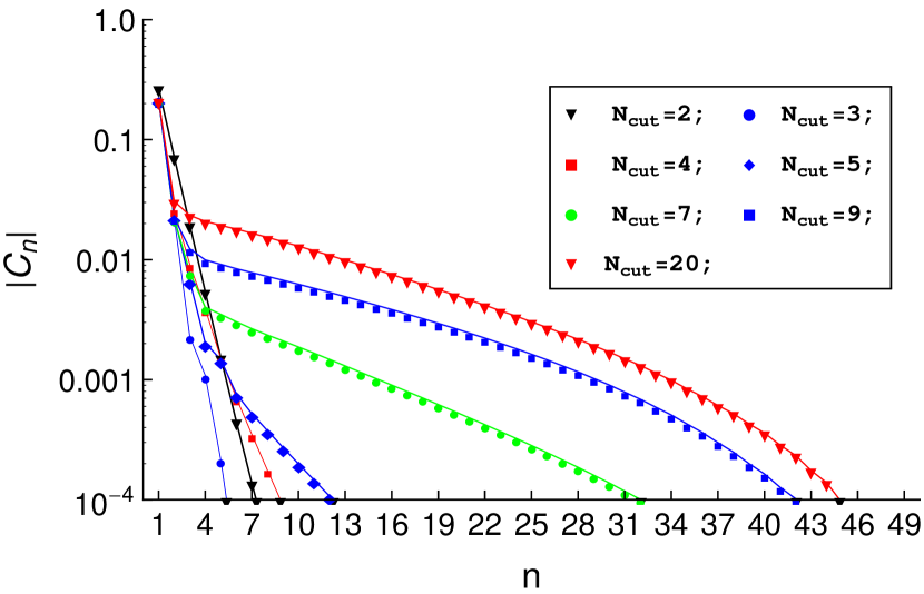
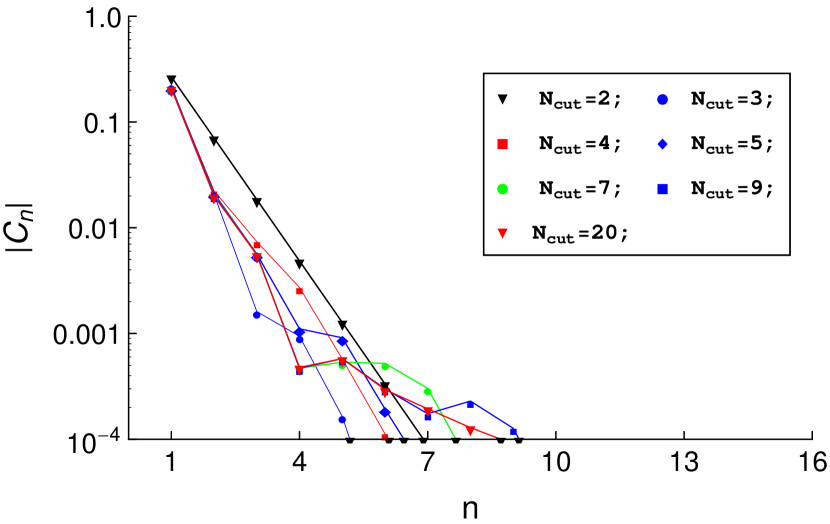
Figure 6: The absolute values of the different space correlation functions for different values of the interaction radius. The chain length is $\displaystyle N=50$ dipoles and $\displaystyle\mu=30\,$MD units, $\displaystyle\gamma=5.0$. In the left panel, the heat flux is generated by the temperature differences of thermostats $\displaystyle T_{L}=0.1\,$MD units, $\displaystyle T_{R}=0.3\,$MD units. In the right panel, the space correlation function in equilibrium conditions is presented, $\displaystyle T=0.2\,$MD units.

One more noteworthy peculiarity of space correlations is observed. Altering the range of dipole-dipole interaction (by changing the cutoff radius $\displaystyle N_{cut}$) strongly affects space correlations in a system. In Fig. 6 we see that the magnitudes of the correlations are substantially different for chains with $\displaystyle N_{cut}=2\div 4$ and $\displaystyle N_{cut}\geq 7$. In Fig. 6 we also show the difference between correlations in equilibrium and nonequilibrium states. It is seen that there is a long range order in nonequilibrium for $\displaystyle N_{cut}\neq 2$ that disappears in equilibrium state. Nevertheless, there is some similarity in correlations for a nearest-neighbor interaction, but even in this case a presence of the heat flux makes the correlations decay slower. For long chains the effect still persists.

This long-range character of the space correlation function is due to the heat flux,and behavior of the equilibrium correlation function supports this conjecture. The right graph in Fig. 6 convincingly demonstrates that without heat flux, i.e., in an equilibrium state, the space correlation function decays fast with distance for the same set of parameters as for nonequilibrium one. The link between the space correlation function and the heat flux originates from the fact that coupling to the thermostats results in the interaction between eigenmodes of the chain Lepri et al. (2003). From Fig. 7, one can see the differences between weak ($\displaystyle\gamma=0.1$) and strong ($\displaystyle\gamma=5.0$) coupling of the chain to thermostats.

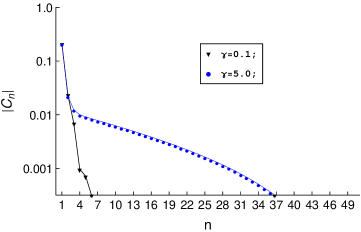
Figure 7: The absolute values of space correlation function in strong and weak coupling regimes. The chain length is $\displaystyle N=50$ dipoles and $\displaystyle\mu=30\,$MD units, $\displaystyle T_{L}=0.1\,$MD units, $\displaystyle T_{R}=0.3\,$MD units, $\displaystyle N_{cut}=9$.

Finally, we consider the influence of the disorder on space correlations. Surprisingly, the effect of the disorder turns out to be not strictly ”destructive”. From the left panel of Fig. 8 we see that for $\displaystyle\sigma=0.01,\,0.1$ correlations are stronger than ones in an ordered chain, whereas for higher values of $\displaystyle\sigma$ they become weaker. To quantitatively estimate this result, we introduce correlation length $\displaystyle\zeta$ defined as a minimal number $\displaystyle n_{\zeta}$ such that $\displaystyle|C_{n_{\zeta}}|<10^{-3}$. Nonmonotonic character of $\displaystyle\zeta(\sigma)$ is evidently seen in the right panel of Fig. 8. This result is very intriguing because from general considerations disorder should break the long-range order in a system. Moreover, it is important to note, that the enhancement of correlations is almost independent on the range of correlations. Correlation functions $\displaystyle C_{n}$ calculated with $\displaystyle N_{cut}=2$ and $\displaystyle N_{cut}=9$ are close enough to say that effect of disorder weakly depends on $\displaystyle N_{cut}$. Another important point is the absence of this effect in equilibrium conditions.

To elucidate the origin of this amplification of long-range correlation by the disorder, we computed the local temperature profile along the dipole chain (Fig. 9). As one can see from Fig. 9, in ordered case ($\displaystyle\sigma=0$) the temperature is flat along the chain and changes only on the interface dipoles. When we introduce a small disorder ($\displaystyle\sigma<0.12$), a linear temperature gradient develops along the entire chain, which couples all dipoles and leads to the increase of the long range correlation. The further increase of a disorder results in a strong localization of a thermal gradient in the middle of the chain, part of dipoles become ”uncoupled” and we observe weakening of the correlations. It is known from a nonequilibrium thermodynamics De Groot and Mazur (2013) that in polarizable media a temperature gradient creates an electric field that raises overall polarization Bresme et al. (2008); Muscatello et al. (2011).

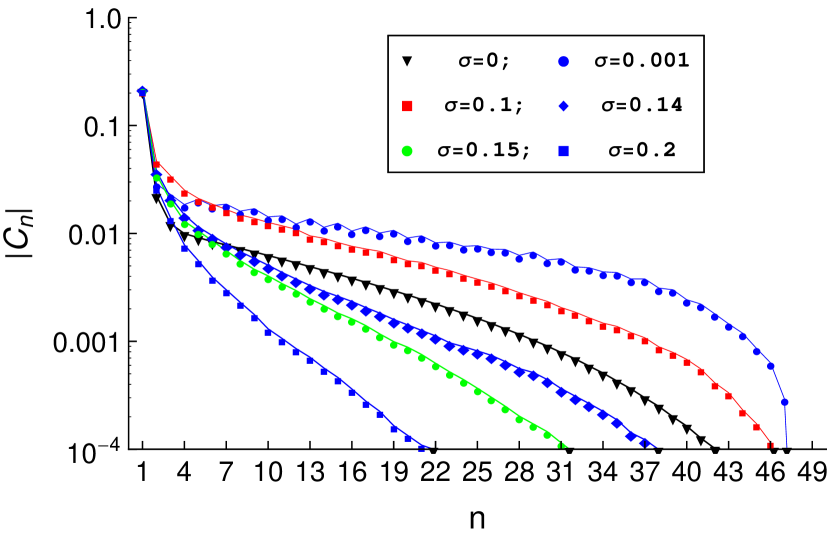
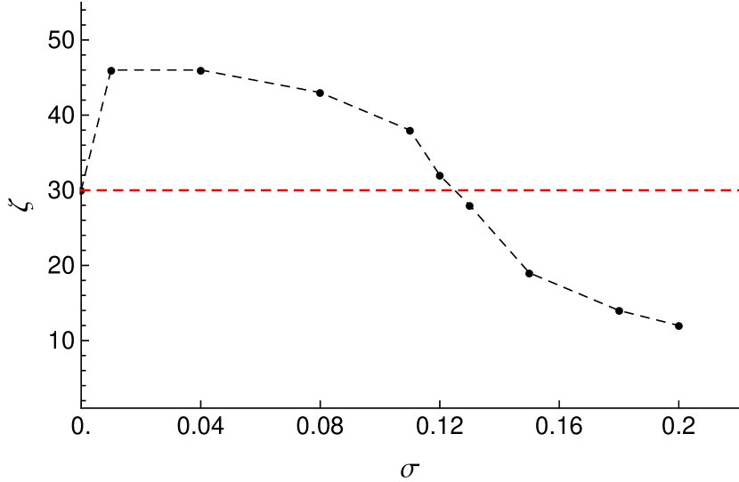
Figure 8: The absolute values of space correlation function for different disorder strengths. The chain length is $\displaystyle N=50$ and $\displaystyle\mu=30\,$MD units, $\displaystyle T_{L}=0.1\,$MD units, $\displaystyle T_{R}=0.3\,$MD units, $\displaystyle N_{cut}=9$. The right panel shows dependence of the correlation length $\displaystyle\zeta$ on the disorder strength is presented. Horizontal dashed line represents the value of a correlation length in ordered chain, $\displaystyle\sigma=0$.

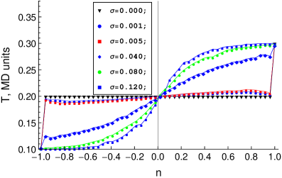
Figure 9: Temperature profiles for different disorder strengths according to Eq. (III.24). Profiles in disordered cases were obtained by averaging over $\displaystyle 200$ disorder realizations, $\displaystyle T_{1}=0.1\,$MD units, $\displaystyle T_{2}=0.3\,$MD units, $\displaystyle N_{cut}=9$.

IV Summary

In the present paper, we have conducted numerical and analytical study of the classical dipolar chain under out-of-equilibrium conditions. We approximated nonequlibrium dynamics of the chain by a system of linearized stochastic differential equations. All the quantities of interest after that were expressed solely through the elements of the one matrix $\displaystyle\mathbf{M}$ Eq. (II.6). We focused on two basic aspects of the chain: heat conduction and correlations.

To study the heat conduction we derived a closed expression for the heat current, Eq. (II.11). It was established that ordered dipole chain supports ballistic transport and their properties resemble ones of the harmonic lattice; e.g., the heat current is proportional to the difference of the thermostats’ temperatures $\displaystyle\Delta T$ and not to the temperature gradient $\displaystyle\Delta T/N$. This fact points to the violation of the Fourier law in ordered dipolar chain. Ballistic transport regime is destroyed by a disorder introduced by a random distribution of dipoles’ positions. We used the simple model where positions of dipoles are imposed to be random Gaussian variables. The dispersion of the distribution plays a role of the disorder’s ”strength”. Within the adopted model of disorder, we calculated the temperature profile and heat conductivity. It was observed that heat conduction undergoes the transition from ballistic to diffusive transport. In the diffusive regime, the heat conductivity decreases as we increase the chain length. Diffusive regime is also characterized by the establishing of the temperature gradient in chain. Deformation of the temperature profile in disordered chain is in good agreement with the recent results on the derivation of the Fourier’s law in quantum wires Dubi and Di Ventra (2009). Similar to the quantum case Dubi and Di Ventra (2009), there are two different length scales in a problem of heat conduction. The first one corresponds to localization length. The second one corresponds to the thermal length. These two lengths can be very different. In the model considered in the present article, estimation of the localization length is complicated by the presence of the strong correlations between eigenmodes. We left this question for further consideration.

We constructed the exact formula for ”dipole-dipole” correlation function Eq. (II.20). This allowed us to estimate the relaxation times and to show the slowing of orientation relaxation as the system size increases (see Fig. 5).

The situation with spatial correlations is more subtle because they are affected by different factors such as thermostats’ temperature difference, dipole moments, and interaction range (cutoff radius $\displaystyle N_{cut}$). The most prominent feature of nonequilibrium is the emergence of the long-range correlations for $\displaystyle N_{cut}>5$. It is especially important because usually the model with only nearest-neighbor interaction is considered in the majority of works in out-of-equilibrium low dimensional systems. Here we clearly demonstrated that long-range behavior of the correlation is caused by the combination of two factors: heat flow and ”long-range” interaction. The nonequilibrium is essential because it leads to the coupling between heat-carrying modes of the systems and the eigenmodes interaction is necessary for the emergence of long-range structure. One can generalize this conclusion by making the conjecture that the emergence of long-range correlations in a one-dimensional system is possible under nonequilibrium conditions when next-nearest-neighbor interactions are included.

V Acknowledgments

This work has been supported by the Belgian Federal Government. The authors thank Maxim Gelin for many valuable discussions.

Appendix A Units of measure adopted in the article

• The value of the dipole moment corresponds to the one of the water in the carbon nanotube and is taken from the molecular dynamics simulation Köfinger and Dellago (2010) : $\displaystyle\mu=1.9975\,D$;

• Length unit: $\displaystyle a=2.65$ Å, ibid;

• Energy unit: $\displaystyle\epsilon=\displaystyle{\frac{\mu^{2}}{a^{3}}}$, with the above values of the dipole moment and lattice spacing we get $\displaystyle\epsilon=2.14406\cdot 10^{-13}\,erg$;

• The unit of time: $\displaystyle\tau=\displaystyle{\sqrt{\frac{Ia^{3}}{\mu^{2}}}}=3.74161\cdot 10^{-14}\,s$, where $\displaystyle I$ is the moment of inertia of a dipole. For $\displaystyle I$ we take the mean value of the three principal values of this tensor of the water molecule Eisenberg and Kauzmann (2005), $\displaystyle I=3.0\cdot 10^{-40}\,g/cm^{2}$;

Appendix B Space correlation function in nonequilibrium steady state

In this section we give some useful formulas that are used for calculation of the space correlation function of one-dimensional lattices Rieder et al. (1967); Nakazawa (1970); Casati (1979). Below we closely follow the work of Ref. Nakazawa (1970).

We start with rewriting the system Eq. (II.4) in the form of the first order differential equation:

$$\dot{\mathbf{x}}=\mathbf{A}\mathbf{x}+\mathbf{F}(t),$$ (B.26)

where the column vector $\displaystyle\mathbf{x}(t)=(\varphi_{1}(t),\ldots,\varphi_{N}(t),p_{1}(t)\ldots p_{N}(t))^{T}$ and

$$A=\begin{pmatrix}\mathbf{0}_{NN}&\phantom{-}\mathbf{I}_{NN}\\ \mathbf{M}&-\mathbf{\Gamma}\end{pmatrix},\quad\Gamma_{ij}=\gamma_{L}\delta_{i1}\delta_{j1}+\gamma_{R}\delta_{iN}\delta_{jN}$$ (B.27)

where $\displaystyle\mathbf{0}_{NN}$ is $\displaystyle N$-by-$\displaystyle N$ zero matrix, $\displaystyle\mathbf{I}_{NN}$ is $\displaystyle N$-by-$\displaystyle N$ identity matrix, $\displaystyle\mathbf{M}$ is the potential energy matrix, $\displaystyle\mathbf{F}=(\mathbf{0}_{N},\eta_{L}(t),0,\ldots,\eta_{R}(t))^{T}$ and $\displaystyle\eta_{L}(t)$, $\displaystyle\eta_{R}(t)$ are Gaussian white noises. Solution of Eq. (B.26) is of the form

$$\mathbf{x}(t)=\exp(\mathbf{A}t)\mathbf{x}(0)+\int\limits_{0}^{t}\exp\Big{(}\mathbf{A}(t-t^{\prime})\Big{)}\mathbf{F}(t^{\prime})\,dt^{\prime},$$ (B.28)

where $\displaystyle\mathbf{x}(0)$ is column of the initial conditions. To find the correlations in the nonequlibrium steady state we have to calculate the limit $\displaystyle\lim_{t\to+\infty}\langle\mathbf{x}(t)\mathbf{x}^{\dagger}(t)\rangle$, where $\displaystyle\langle\mathbf{x}(t)\mathbf{x}^{\dagger}(t)\rangle$ is the covariance matrix. It can be done by employing the fact that all eigenvalues of the matrix $\displaystyle\mathbf{A}$ have negative real parts Rieder et al. (1967); Nakazawa (1970) which gives $\displaystyle\lim_{t\to+\infty}\exp(\mathbf{A}t)=0$. After this remark the evaluation of the limit above is done in a straightforward manner:

$$\lim_{t\to+\infty}\langle\mathbf{x}(t)\mathbf{x}^{\dagger}(t)\rangle=\begin{pmatrix}\boldsymbol{\Phi}&\mathbf{Z}\\ \mathbf{Z}^{\dagger}&\mathbf{T}\end{pmatrix}=\int\limits_{0}^{\infty}\exp(\mathbf{A}t)\mathbf{D}\exp(\mathbf{A}^{\dagger}t)\,dt,$$ (B.29)

where

$$\langle\mathbf{F}(t)\mathbf{F}^{\dagger}(t^{\prime})\rangle=\mathbf{D}\delta(t-t^{\prime})=\begin{pmatrix}\mathbf{0}_{NN}&\mathbf{0}_{NN}\\ \mathbf{0}_{NN}&\mathbf{\Delta}\end{pmatrix}\delta(t-t^{\prime}),\quad\Delta_{ij}=2\gamma_{L}T_{L}\delta_{i1}\delta_{j1}+2\gamma_{R}T_{R}\delta_{iN}\delta_{jN},$$ (B.30)

$$\boldsymbol{\Phi}=\langle\boldsymbol{\varphi}\boldsymbol{\varphi}^{\dagger}\rangle,\quad\mathbf{Z}=\langle\boldsymbol{\varphi}\boldsymbol{p}^{\dagger}\rangle,\quad\mathbf{T}=\langle\boldsymbol{p}\boldsymbol{p}^{\dagger}\rangle.$$

Here we have used the fluctuation-dissipation theorem Eq. (II.3) and definition of $\displaystyle\mathbf{F}(t)$ given above. The matrices $\displaystyle\boldsymbol{\Phi}$, $\displaystyle\mathbf{Z}$ and $\displaystyle\mathbf{T}$ represent space correlation function, mean heat flux, and temperature profile (diagonal elements of $\displaystyle\mathbf{T}$) respectively. The correlation function can be obtained by direct calculation of the integral Eq. (B.29) by the method developed in Ref. Van Loan (1978). It can be also helpful to rewrite Eq. (B.29) in the matrix form Rieder et al. (1967); Nakazawa (1970):

$$\mathbf{A}\mathbf{C}+\mathbf{C}\mathbf{A}^{\dagger}=-\mathbf{D},$$ (B.31)

with $\displaystyle\mathbf{C}$ being $\displaystyle\langle\mathbf{x}(+\infty)\mathbf{x}^{\dagger}(+\infty)\rangle$. An exact solution of this equation was found only for the nearest-neighbor interaction. From a general point of view, it is a well known in a control theory Lyapunov matrix equation and number of algorithms were developed to solve it numerically Golub et al. (1979); Wachspress (1988); Penzl (1998).

Appendix C The inverse of the matrix M and calculation of the heat current

In the Langevin dynamics we calculate two main quantities: heat current, Eq. (II.11), and the correlation function, Eq. (II.19). In both cases, the formulas contain the elements of the inverse matrix $\displaystyle\mathbf{M}^{-1}$ that, by definition, is given by

$$\mathbf{M}^{-1}=\frac{1}{\det\mathbf{M}}\mathbf{C}^{\mathrm{T}},$$ (C.32)

where $\displaystyle\mathbf{C}$ is the matrix of cofactors Gantmacher (1960) and $\displaystyle\mathrm{T}$ stands for transposition. Due to the $\displaystyle\mathbf{M}$ being symmetric a matrix, the matrix of cofactors $\displaystyle\mathbf{C}$ is also symmetric.

The integrands in Eq. (II.19) and Eq. (II.11) are the rational functions and the order of the polynomial in the denominator is $\displaystyle 2N$ (see comments at the end of the Sec. II.1). From general considerations, it follows that there should be no zeros of the $\displaystyle\det{\mathbf{M}}(\omega)$ on the real axis because if there were even one the integral in Eq. (II.11) became ambiguous while the heat current is a physically observable quantity and must be defined unambiguously.

Now, we are ready to calculate the integral

$$\langle j\rangle=\frac{2\gamma_{L}\gamma_{R}\Delta T}{2\pi}\int\limits_{-\infty}^{+\infty}\omega^{2}|(M^{-1})_{1N}(\omega)|^{2}\,d\omega.$$ (C.33)

From the residue theorem, it immediately follows Ablowitz and Fokas (2003):

$$\langle j\rangle=2\pi i\frac{2\gamma_{L}\gamma_{R}\Delta T}{2\pi}\sum\limits_{\omega_{i}}\mathop{\mathrm{Res}}\limits_{\omega=\omega_{i}}\left(\omega^{2}\frac{\mathbf{C}_{N1}(\omega)\mathbf{C}_{N1}(-\omega)}{\det\mathbf{M}(\omega)\det\mathbf{M}(-\omega)}\right),$$ (C.34)

where $\displaystyle\omega_{i}$ satisfies the equation

$$\det\mathbf{M}(\omega_{i})=0,$$ (C.35)

in the half-plane $\displaystyle\mathrm{Im}\,\omega<0$ and $\displaystyle\mathop{\mathrm{Res}}\limits_{\omega=\omega_{i}}$ states for the residue at the point $\displaystyle\omega=\omega_{i}$. The determinant can be represented in the form of a product:

$$\det\mathbf{M}(\omega)=\prod\limits_{i=1}^{2N}(\omega-\omega_{i}).$$ (C.36)

It is tacitly supposed that roots of this polynomial are simple. This assumption is based on the results of the numerical computations: for all considered chain lengths, the roots are found to be simple and all lie in the lower half-plane of the $\displaystyle\omega$-plane, Fig. 10. Hence, poles in Eq. (C.34) are simple and calculation of the sum can be done easily. To be assured we checked the teh multiplicity of the roots in the Multroot package Zeng (2004) yielded the same conclusion.

Figure 10: Zeros of $\displaystyle\det\mathbf{M}(\omega)$ for different $\displaystyle N_{cut}$; $\displaystyle\bullet$ correspond to $\displaystyle N_{cut}=3$, $\displaystyle\blacktriangledown$ correspond to $\displaystyle N_{cut}=20$; $\displaystyle N=50$, $\displaystyle\mu=1.0\,$MD units

At the end of the section we will show how to tackle the root-finding of the $\displaystyle\det\mathbf{M}(\omega)$. As it was already said, this polynomial has large coefficients and is of the order of $\displaystyle 2N$. Hence, it is a cumbersome problem to find its roots. Nevertheless, it can be greatly simplified by the following observation.

Applying the Fourier transform to Eq. (B.26), we get the matrix equation:

$$-\mathrm{i}\omega\mathbf{x}(\omega)=\mathbf{A}\mathbf{x}(\omega)+\mathbf{F}(\omega).$$ (C.37)

Thus, a particular solution of Eq. (B.26) is

$$\mathbf{x}(t)=\frac{1}{2\pi}\int\limits_{-\infty}^{+\infty}\exp(-\mathrm{i}\omega t)\mathbf{x}(\omega)\,d\omega=-\frac{1}{2\pi}\int\limits_{-\infty}^{+\infty}\frac{\exp(-\mathrm{i}\omega t)}{\mathrm{i}\omega\mathbf{I}+\mathbf{A}}\mathbf{F}(\omega)\,d\omega,$$ (C.38)

where $\displaystyle\mathbf{I}$ is $\displaystyle 2N$-by-$\displaystyle 2N$ identity matrix. Comparison of this expression with the inverse Fourier transform Eq. (II.5) shows that zeros of $\displaystyle\det\mathbf{M}(\omega)$ coincide with zeros of $\displaystyle\det(\mathrm{i}\omega\mathbf{I}+\mathbf{A})$ and the latter are equal to $\displaystyle\mathrm{i}\lambda_{k}$, $\displaystyle k=1,2\ldots 2N$, where $\displaystyle\lambda_{k}$ is the $\displaystyle k$-th eigenvalue of the $\displaystyle\mathbf{A}$. Therefore,

$$\det\mathbf{M}(\omega_{k})=0,\quad\forall\,\omega_{k}=\mathrm{i}\lambda_{k},\;k=1,2,\ldots,2N.$$ (C.39)

According to this observation, the determinant of the $\displaystyle\mathbf{M}(\omega)$ in Eq. (C.34) can be evaluated as

$$\det\mathbf{M}(\omega)=\prod\limits_{k=1}^{2N}(\omega-\mathrm{i}\lambda_{k}).$$ (C.40)

The problem of finding eigenvalues of the nonsingular matrix is well known and can be implemented in a robust and reliable way.

Now, when we know that all zeros of $\displaystyle\det\mathbf{M}(\omega)$ are simple and know the relation between them and eigenvalues of $\displaystyle\mathbf{A}$, we can calculate the residue in Eq. (C.34):

$$\langle j\rangle=2\mathrm{i}\gamma_{L}\gamma_{R}\Delta T\sum\limits_{n=1}^{2N}(\mathrm{i}\lambda_{n})^{2}\frac{\mathbf{C}_{N1}(\mathrm{i}\lambda_{n})\mathbf{C}_{N1}(-\mathrm{i}\lambda_{n})}{\det^{\prime}\mathbf{M}(\mathrm{i}\lambda_{n})\det\mathbf{M}(-\mathrm{i}\lambda_{n})},$$ (C.41)

where $\displaystyle\det\nolimits^{\prime}\mathbf{M}(\mathrm{i}\lambda_{n})=\mathrm{i}\prod\limits_{\begin{subarray}{c}k=1\\ k\neq n\end{subarray}}^{2N}(\lambda_{n}-\lambda_{k})$.

Appendix D Energy current in dipole chain

We begin with the rate of the energy change in chain Lepri et al. (2003); Dhar (2008):

$$\frac{dE}{dt}=\sum\limits_{i=1}^{N}\dot{p_{i}}p_{i}+\frac{1}{2}\sum\limits_{i,j}^{N}\left(\frac{\partial U}{\partial\varphi_{i}}\dot{\varphi_{i}}+\frac{\partial U}{\partial\varphi_{j}}\dot{\varphi_{j}}\right)=\sum\limits_{i,j}F_{ij}p_{i}-\frac{1}{2}\sum\limits_{i,j}^{N}\left(F_{ij}p_{i}+F_{ji}p_{j}\right).$$ (D.42)

The energy change rate for the $\displaystyle i$-th dipole is:

$$\frac{d\epsilon_{i}}{dt}=\frac{1}{2}p_{i}\sum\limits_{j}F_{ij}-\frac{1}{2}\sum\limits_{j}F_{ji}p_{j}.$$ (D.43)

Rewrite it in the following form:

$$\frac{d\epsilon_{i}}{dt}+\left(j_{i}^{in}-j_{i}^{out}\right)=0,$$ (D.44)

where

$$j_{i}^{in}=\frac{1}{2}p_{i}\sum\limits_{j=1}^{N}F_{ij},\quad j_{i}^{out}=\frac{1}{2}\sum\limits_{j=1}^{N}F_{ji}p_{j}.$$ (D.45)

In steady state, the $\displaystyle\left\langle\frac{d\epsilon_{i}}{dt}\right\rangle=0$, thus $\displaystyle\langle j_{i}^{in}\rangle=\langle j_{i}^{out}\rangle$ for every index $\displaystyle i$, where $\displaystyle\langle\phantom{x}\rangle$ stands for the ensemble average. The $\displaystyle j_{i}^{in}$, $\displaystyle j_{i}^{out}$ can be treated as the in, out - heat currents of $\displaystyle i$th dipole, respectively. In a straightforward manner it can be shown Lepri et al. (2003); Dhar (2008) that ”in” steady state in-currents are equal for all dipoles in chain:

$$j_{2}=\frac{1}{2}p_{2}F_{21}=j_{3}=\frac{1}{2}p_{3}\sum\limits_{i=1}^{2}F_{3i}=\ldots=j_{N}=\frac{1}{2}p_{N-1}\sum\limits_{j=1}^{N-1}F_{N-1,j}.$$ (D.46)

Evidently, all these currents in steady state are equal to the energy flowed into the system from the ”hot” thermostat per unit of time and flowed out into the ”cold” thermostat. Equation (D.46) states that the average rate of work done by the $\displaystyle i$th dipole on the followed dipoles is equal to the rate of work done by the previous dipoles on the $\displaystyle i$th. Thus, one can say that the energy flow from the previous dipoles to the $\displaystyle i$th is equal to the energy flow from the $\displaystyle i$th dipole to the followed ones.

References

- Bonetto et al. (2000) F. Bonetto, J. Lebowitz, and L. Rey-Bellet, arXiv preprint math-ph/0002052 (2000).
- Dubi and Di Ventra (2009) Y. Dubi and M. Di Ventra, Physical Review E 79, 042101 (2009).
- Dubi and Di Ventra (2009) Y. Dubi and M. Di Ventra, Physical Review B 79, 115415 (2009).
- Dubi and Di Ventra (2011) Y. Dubi and M. Di Ventra, Rev. Mod. Phys. 83, 131 (2011).
- Reimann (2002) P. Reimann, Phys. Rep. 361, 57 (2002).
- Hänggi (2009) P. Hänggi, Rev. Mod. Phys. 81, 387 (2009).
- Gelin and Kosov (2008) M. F. Gelin and D. S. Kosov, Phys. Rev. E 78, 011116 (2008).
- Kottas et al. (2005) G. S. Kottas, L. I. Clarke, D. Horinek, and J. Michl, Chem. Rev. 105, 1281 (2005).
- de Jonge et al. (2007) J. J. de Jonge, M. A. Ratner, and S. W. de Leeuw, J. Phys. Chem. C 111, 3770 (2007).
- Horansky et al. (2006) R. D. Horansky, L. I. Clarke, E. B. Winston, J. C. Price, S. D. Karlen, P. D. Jarowski, R. Santillan, and M. A. Garcia-Garibay, Phys. Rev. B 74, 054306 (2006).
- Ford (1992) J. Ford, Phys. Rep. 213, 271 (1992).
- Aubry (2006) S. Aubry, Physica D 216, 1 (2006).
- Eckmann et al. (1999) J.-P. Eckmann, C.-a. Pillet, and L. Rey-Bellet, Commun. Math. Phys. 201, 657 (1999).
- Shelton (2005) D. P. Shelton, J. Chem. Phys. 123, 084502 (2005).
- Murashov et al. (2002) V. V. Murashov, P. J. Camp, and G. N. Patey, J. Chem. Phys. 116, 6731 (2002).
- Klapp (2005) S. H. L. Klapp, J. Phys.: Condens. Matter 17, R525 (2005).
- Hummer et al. (2001) G. Hummer, J. C. Rasaiah, and J. P. Noworyta, Nature 414, 188 (2001).
- Köfinger et al. (2008) J. Köfinger, G. Hummer, and C. Dellago, Proc. Nat. Acad. Sci. USA 105, 13218 (2008).
- Kyakuno et al. (2011) H. Kyakuno, K. Matsuda, H. Yahiro, Y. Inami, T. Fukuoka, Y. Miyata, K. Yanagi, Y. Maniwa, H. Kataura, T. Saito, M. Yumura, and S. Iijima, J. Chem. Phys. 134, 244501 (2011).
- Alexiadis and Kassinos (2008) A. Alexiadis and S. Kassinos, Chem. Rev. 108, 5014 (2008).
- Köfinger et al. (2011) J. Köfinger, G. Hummer, and C. Dellago, Phys. Chem. Chem. Phys. 13, 15403 (2011).
- Köfinger et al. (2009) J. Köfinger, G. Hummer, and C. Dellago, J. Chem. Phys. 130, 154110 (2009).
- Kuramoto (1984) Y. Kuramoto, Chemical oscillations, waves, and turbulence (Springer-Verlag, Berlin New York, 1984).
- Acebrón et al. (2005) J. A. Acebrón, L. L. Bonilla, C. J. Pérez Vicente, F. Ritort, and R. Spigler, Rev. Mod. Phys. 77, 137 (2005).
- Lahaye et al. (2009) T. Lahaye, C. Menotti, L. Santos, M. Lewenstein, and T. Pfau, Rep. Prog. Phys. 72, 126401 (2009).
- Arkhipov et al. (2005) A. S. Arkhipov, G. Astrakharchik, A. V. Belikov, and Y. E. Lozovik, JETP Letters 82, 41 (2005).
- Lepri et al. (2003) S. Lepri, R. Livi, and A. Politi, Phys. Rep. 377, 1 (2003).
- Dhar (2008) A. Dhar, Adv. Phys. 57, 457 (2008).
- Coffey et al. (2004) W. Coffey, Y. Kalmykov, and J. Waldron, The Langevin equation: with applications to stochastic problems in physics, chemistry, and electrical engineering, Vol. 14 (World Scientific Publishing Company Incorporated, 2004).
- Casher and Lebowitz (1971) A. Casher and J. Lebowitz, J. Math. Phys. 12, 1701 (1971).
- Dhar and Roy (2006) A. Dhar and D. Roy, J. Stat. Phys. 125, 801 (2006).
- Kampen (1992) v. N. G. Kampen, Stochastic processes in physics and chemistry (North-Holland, Amsterdam New York, 1992).
- Prosen and Campbell (2005) T. Prosen and D. K. Campbell, Chaos (Woodbury, N.Y.) 15, 15117 (2005).
- Anderson (1958) P. W. Anderson, Phys. Rev. 109, 1492 (1958).
- Resta (2011) R. Resta, Eur. Phys. J. B 79, 121 (2011).
- Bussi and Parrinello (2007) G. Bussi and M. Parrinello, Phys. Rev. E 75, 056707 (2007).
- Dhar and Lebowitz (2008) A. Dhar and J. L. Lebowitz, Phys. Rev. Lett. 100, 134301 (2008).
- Evers and Mirlin (2008) F. Evers and A. D. Mirlin, Rev. Mod. Phys. 80, 1355 (2008).
- De Groot and Mazur (2013) S. R. De Groot and P. Mazur, Non-equilibrium thermodynamics (Courier Dover Publications, 2013).
- Bresme et al. (2008) F. Bresme, A. Lervik, D. Bedeaux, and S. Kjelstrup, Phys. Rev. Lett. 101, 020602 (2008).
- Muscatello et al. (2011) J. Muscatello, F. Romer, J. Sala, and F. Bresme, Phys. Chem. Chem. Phys. 13, 19970 (2011).
- Köfinger and Dellago (2010) J. Köfinger and C. Dellago, New J. Phys. 12, 093044 (2010).
- Eisenberg and Kauzmann (2005) D. Eisenberg and W. Kauzmann, The structure and properties of water (Oxford Clarendon Press, 2005).
- Rieder et al. (1967) Z. Rieder, J. Lebowitz, and E. Lieb, J. Math. Phys. 8, 1073 (1967).
- Nakazawa (1970) H. Nakazawa, Suppl. Progr. Theor. Phys 45, 231 (1970).
- Casati (1979) G. Casati, Nuovo Cimento B 52, 257 (1979).
- Van Loan (1978) C. Van Loan, Automatic Control, IEEE Transactions on 23, 395 (1978).
- Golub et al. (1979) G. Golub, S. Nash, and C. Van Loan, Automatic Control, IEEE Transactions on 24, 909 (1979).
- Wachspress (1988) E. L. Wachspress, Appl. Math. Lett. 1, 87 (1988).
- Penzl (1998) T. Penzl, Adv. Comput. Math. 8, 33 (1998).
- Gantmacher (1960) F. Gantmacher, Theory of Matrices (Chelsea, New York, 1960).
- Ablowitz and Fokas (2003) M. Ablowitz and A. Fokas, Complex variables: introduction and applications (Cambridge University Press, 2003).
- Zeng (2004) Z. Zeng, ACM Trans. Math. Softw. 30, 218 (2004).