Renormalization Group Flow of Hexatic Membranes

Abstract

We investigate hexatic membranes embedded in Euclidean $D$-dimensional space using a re–parametrization invariant formulation combined with exact renormalization group (RG) equations. An XY–model coupled to a fluid membrane, when integrated out, induces long–range interactions between curvatures described by a Polyakov term in the effective action. We evaluate the contributions of this term to the running surface tension, bending and Gaussian rigidities in the approximation of vanishing disclination (vortex) fugacity. We find a non–Gaussian fixed–point where the membrane is crinkled and has a non–trivial fractal dimension.

.1 Introduction

Hexatic membranes are a very interesting example of physical system which undergoes a non–trivial phase transition induced by a combination of geometrical and topological interactions Nelson_Piran_Weinberg_1988 . This system is even more interesting since it is characterized by local re–parametrization invariance, and is thus an example of a theory characterized by local symmetries with a renormalization group (RG) flow exhibiting a non–Gaussian fixed point in two dimensions.

In the continuum, Hexatic membranes are described as a fluid membrane coupled to an $O(2)$–symmetric scalar field. The $O(2)$–global symmetry represents in the continuum the $\mathbb{Z}_{6}$–symmetry characteristic of the orientational order of triangular or hexagonal lattices (from this last it takes the name) that melt Nelson_Piran_Weinberg_1988 ; the $O(2)$–symmetric scalar field plays thus the role of the orientational order parameter. Hexatic membranes are effectively described by combining the fluid membrane and the $O(2)$–model actions:

$$S[\mathbf{N},\mathbf{r}]=\int d^{2}x\sqrt{g}\left\{\mu+\frac{\kappa}{2}K^{2}+\frac{\bar{\kappa}}{2}R\right\}\qquad$$

$$+\frac{K_{A}}{2}\int d^{2}x\sqrt{g}\,\nabla_{\alpha}\mathbf{N}\cdot\nabla^{\alpha}\mathbf{N}\,.$$ (1)

In (1) $K_{A}$ is the hexatic stiffness, $\mu$ is the surface tension, $\kappa$ is the bending rigidity and $\bar{\kappa}$ is the Gaussian rigidity Nelson_Piran_Weinberg_1988 . The action (1) is invariant under re–parametrization of the embedding field $\mathbf{r}:\mathbb{R}^{2}\rightarrow\mathbb{R}^{D}$; $g_{\mu\nu}=\partial_{\mu}\mathbf{r}\cdot\partial_{\nu}\mathbf{r}$ is the induced metric, $K^{2}$ is the square of the trace of the extrinsic curvature, while $R$ is the intrinsic Gaussian curvature. The scalar field, tangent to the surface, is constrained to have unit length $\mathbf{N}\cdot\mathbf{N}=1$.

In this paper we study the RG flow of the couplings appearing in the action (1) by computing their beta functions for arbitrary embedding dimension $D$. Differently from previous approaches to hexatic membranes Nelson_Peliti_1987 ; David_Guitter_Peliti_1987 ; Guitter , we use a geometrical formulation of the model which is explicitly covariant and we apply to it the effective average action formalism Berges:2000ew , which has been adapted to fluid membranes in Codello_Zanusso_2011 . The phase diagram of fluid membranes is modified by the inclusion of the hexatic stiffness, which induces, in the RG flow, a non–Gaussian IR fixed–point at which the surface is crinkled, i.e. it has a non–trivial finite fractal dimension David_Guitter_Peliti_1987 .

The $O(2)$–action in (1) can also be seen as the generalization on a membrane of the continuum action describing the XY–model. As it is well know, the XY–model is subject to the Kosterlitz–Thouless topological phase transition Kosterlitz , mediated by the unbinding of vortices. In the context of hexatic membranes, disclinations Nelson_Piran_Weinberg_1988 are the relevant topological excitations; these interact by long–range Coulomb interactions, and in this way they affect the phase behavior of the model. Interestingly, also the Gaussian curvature plays a similar role, since it is a source of frustration for the field $\mathbf{N}$, which, when parallel transported around a closed loop, is shifted proportionally to the total Gaussian curvature enclosed. This is described by long–range Coulomb interactions between Gaussian curvatures in the form of a Polyakov term $\int\sqrt{g}R\frac{1}{\Delta}R$ Polyakov:1981rd , resulting from the integration of the $O(2)$–field.

Even if, in the effective average action formalism, it is possible to account for the effect of topological defects without explicitly summing over them Grater:1994qx , in this paper we will discard the contribution of disclinations and focus on the effect that the long–range Coulomb interactions between Gaussian curvatures have on the phase diagram. Our main interest is to understand the effect that non–local invariants have on the RG flow of the couplings of the local ones. As we will see, it is the hexatic stiffness $K_{A}$, seen as the coupling of the Polyakov term, that has the effect of changing the phase structure of fluid membranes by modifying the beta functions of the bending rigidity.

.2 Induced long-range curvature–curvature interactions

At every point of the membrane we can introduce zwei-bein orthonormal vector fields $\mathbf{e}_{a}=e^{\alpha}_{a}\partial_{\alpha}\mathbf{r}$ such that $e^{\alpha}_{a}e^{\beta}_{b}g_{\alpha\beta}=\delta_{ab}$. Covariant derivatives of the zwei-beins define the spin connection $\omega_{\alpha ab}$ through the relation $\nabla_{\alpha}\mathbf{e}_{a}=\omega_{\alpha ab}\mathbf{e}_{b}$, which describes how the zwei-beins rotates under parallel transport. We can now write the vector field $\mathbf{N}$ in the zwei-bein basis $\mathbf{N}=\cos\theta\,\mathbf{e}_{1}+\sin\theta\,\mathbf{e}_{2}$, defining in this way the angle variable $\theta$, in terms of which the action (1) becomes:

$$S[\theta,\mathbf{r}]=\int d^{2}x\sqrt{g}\left\{\mu+\frac{\kappa}{2}K^{2}+\frac{\bar{\kappa}}{2}R\right\}\qquad\qquad$$

$$+\frac{K_{A}}{2}\int d^{2}x\sqrt{g}\,(\partial_{a}\theta+\omega_{a})(\partial^{a}\theta+\omega^{a})\,.$$ (2)

The angle $\theta$ parametrizes the one dimensional sphere $O(2)=S^{1}$. Since the field $\theta$ appears quadratically, we can complete the square to perform the Gaussian integral obtaining in this way an effective action for the membrane alone. This amounts in shifting the field $\theta\rightarrow\theta-\int\frac{1}{\Delta}\nabla_{a}\omega^{a}$ of the amount given by the solution of the tree–level equation of motion $\Delta\theta+\nabla_{a}\omega^{a}=0$, where $\Delta\equiv-g^{\alpha\beta}\nabla_{\alpha}\nabla_{\beta}$ is the covariant Laplacian. After using the relation between the Gaussian curvature and the spin connection, $R=\frac{2}{\sqrt{g}}\epsilon_{ab}\nabla^{a}\omega^{b}$, one finds that the action (2) becomes:

$$S[\theta,\mathbf{r}] =\int d^{2}x\sqrt{g}\left\{\mu+\frac{\kappa}{2}K^{2}+\frac{\bar{\kappa}}{2}R\right\}$$ (3)

$$+\frac{K_{A}}{2}\int d^{2}x\sqrt{g}\,\partial_{a}\theta\partial^{a}\theta$$

$$+\frac{K_{A}}{8}\int d^{2}x\sqrt{g}R\frac{1}{\Delta}R\,.$$

The step between (2) and (3) is analogous to what happens in Liouville theory, where the Gaussian action $\int\sqrt{g}\left(\frac{1}{2}\phi\Delta\phi+\phi R\right)$ gives rise to a Polyakov term with both classical and quantum contributions. In the Liouville case one makes the shift $\phi\rightarrow\phi-\int\frac{1}{\Delta}R$ obtained by solving the tree–level equation of motion $\Delta\phi+\phi R=0$. The underlining idea is that the tree–level equations of motion directly give the correct change of variables to complete the square in a Gaussian integral.

The $O(2)$–field has the effect of inducing long–range interactions between Gaussian curvature; these are represented in (3) by a term proportional to the Polyakov effective action. At this point, as done in David_Guitter_Peliti_1987 , one can integrate out the field $\theta$ to obtain the hexatic membrane effective action:

$$S_{eff}[\mathbf{r}]=\int d^{2}x\sqrt{g}\left\{\mu_{0}+\frac{\kappa_{0}}{2}K^{2}+\frac{\bar{\kappa}_{0}}{2}R\right\}$$

$$+\frac{K_{A,0}}{8}\int d^{2}x\sqrt{g}R\frac{1}{\Delta}R\,,$$ (4)

with renormalized $\mu_{0}$, $\bar{\kappa}_{0}$ (the bending rigidity is not renormalized $\kappa_{0}=\kappa_{\infty}$) and finitely renormalized hexatic stiffness:

$$K_{A,0}=K_{A,\infty}-\frac{1}{12\pi}\,.$$ (5)

One can obtain (4) using the effective average action formalism along the lines of Codello_2010 , where it was shown how the Polyakov action arises as field modes are integrated out, one by one, from the UV to IR, and resulting in (5).

.3 Flow equation and beta functions

The effective average action is a functional that depends on an infrared scale $k$ and that interpolates smoothly between the bare, or microscopic, action for $k\rightarrow\infty$ and the full effective action for $k\rightarrow 0$; when local symmetries are present it is constructed using the background field method. The adaptation of the formalism to fluid membranes has already been done Codello_Zanusso_2011 to which we refer for more details. For a complementary study of polymerized membranes using the effective average action approach see Kownacki_Mouhanna_2009 . One can construct a functional $\Gamma_{k}\left[\mathbf{r}\right]$ such that it is a re–parametrization invariant functional of the embedding field $\mathbf{r}$ of the membrane.

The main advantage of working with the effective average action formalism is that we dispose of an exact RG flow equation that describes its scale derivative ($t=\log k$):

$$\partial_{t}\Gamma_{k}[\mathbf{r}]=\frac{1}{2}\textrm{Tr}\frac{\partial_{t}R_{k}(\Delta)}{\Gamma_{k}^{(2)}[\mathbf{r}]+R_{k}(\Delta)}\,.$$ (6)

In (6) $\Gamma_{k}^{(2)}[\mathbf{r}]$ represents the Hessian obtained by expanding the effective average as $\mathbf{r}\rightarrow\mathbf{r}+\nu^{i}\mathbf{n}^{i}$ to second order in the fluctuation fields $\nu^{i}$. Here $\nu^{i}$, with $i=D-2$, are the fluctuations in the direction of the $\mathbf{n}^{i}$ normals vectors and the function $R_{k}(\Delta)$ is the cutoff kernel. The derivation of the flow equation (6) is also given Codello_Zanusso_2011 .

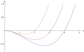
Figure 1: Beta function of the coupling $\alpha_{k}$ for (from bottom) $K_{A}=\frac{1}{2},1,2$.

To proceed we need to make a truncation ansatz for the effective average action in order to project the RG flow to a treatable finite dimensional subspace. We choose the scale dependent version of (4):

$$\Gamma_{k}[\mathbf{r}]=\int d^{2}x\sqrt{g}\left\{\mu_{k}+\frac{\kappa_{k}}{2}K^{2}+\frac{\bar{\kappa}_{k}}{2}R\right\}$$

$$+\frac{K_{A,k}}{8}\int d^{2}x\sqrt{g}R\frac{1}{\Delta}R\,,$$ (7)

where we introduced the running surface tension $\mu_{k}$, the running bending $\kappa_{k}$ and Gaussian $\bar{\kappa}_{k}$ rigidities.

The hexatic stiffness $K_{A,k}$ does not renormalize, i.e. its beta function is zero:

$$\partial_{t}K_{A,k}=0\,.$$ (8)

One way to see this, following the arguments of David_Guitter_Peliti_1987 , is to consider the Polyakov term in the effective action (4) as the result of the integration of $N$ free scalar fields; then $N=K_{A,0}=K_{A,\infty}-\frac{1}{12\pi}$ is preserved by fluctuations. Another way to reach the same conclusion is to consider the $\theta$ scalar field as a non–linear sigma model on $O(2)=S^{1}$. The beta function of $K_{A,k}$ is then proportional to the Gaussian curvature of $S^{1}$ Codello:2008qq , which is identically zero since the manifold is one–dimensional. A third argument is related to the flow of the Polyakov action. In Codello_2010 it is shown that the RG flow induced by a minimally coupled scalar, as is $\theta$, induces a Polyakov term in the effective average action only in the limit $k\rightarrow 0$; thus for non–zero $k$, the flow of $K_{A,k}$, as extracted form the Polyakov term, is zero. In the following we will consider $K_{A,k}=K_{A}$ as a parameter. As in the standard Kosterlitz–Thouless topological phase transition, the flow of the hexatic stiffness is induced by topological defects (here the disclinations) Park_Lubensky_1996a . We will discuss this in a future work Codello_Mouhanna_Zanusso_2013 .

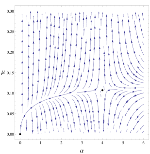
Figure 2: The flow in the $(\alpha_{k},\tilde{\mu}_{k})$ plane for $D=3$ and $K_{A}=1$. The Gaussian and non–Gaussian fixed points are marked dots.

To obtain the projected flow for the couplings in (7) we proceed as in Codello_Zanusso_2011 with the difference that we need to determine the contribution of the hexatic stiffness to the running couplings, i.e. we need to compute the terms proportional to $\int\sqrt{g}$, $\int\sqrt{g}K^{2}$ and $\int\sqrt{g}R$ on the rhs of the flow equation (6) generated by the Hessian of the Polyakov term in (7). We report the details of the computation of the Hessian in the appendix. Following the notation of Codello_Zanusso_2011 , we find:

$$\Gamma_{k}^{(2)}[\mathbf{r}]_{ij} = \left(\kappa_{k}\Delta^{2}+\mu_{k}\Delta\right)\delta_{ij}+\left(V_{ij}^{\alpha\beta}+W_{ij}^{\alpha\beta}\right)\nabla_{\alpha}\nabla_{\beta}$$ (9)

$$+\,U_{ij}+O(K^{4})\,,$$

where $V_{ij}^{\alpha\beta}$ and $U_{ij}$ are as in Codello_Zanusso_2011 and

$$W_{ij}^{\alpha\beta}=K_{A}\left[\frac{1}{2}\delta_{ij}R+\frac{1}{2}K^{i}K^{j}+K_{\gamma\delta}^{i}K^{j}{}^{\gamma\delta}\right]g^{\alpha\beta}\,,$$ (10)

is the contribution to the Hessian coming form the Polyakov action. In (9) and (10) we kept terms up to order $K^{2}$ and $R$. Following the procedure of Codello_Zanusso_2011 to perform the functional trace and using the contraction $g_{\alpha\beta}W_{ii}^{\alpha\beta}=K_{A}\left[2\left(D-3\right)R+3K^{2}\right]$, finally gives the beta functions:

$$\partial_{t}\mu_{k} = \frac{D-2}{8\pi}Q_{1}\left[G_{k}\partial_{t}R_{k}\right]$$

$$\partial_{t}\kappa_{k} = \frac{D}{8\pi}Q_{2}\left[G_{k}^{2}\partial_{t}R_{k}\right]\kappa_{k}-\frac{3}{32\pi}Q_{2}\left[G_{k}^{2}\partial_{t}R_{k}\right]K_{A}$$

$$\partial_{t}\bar{\kappa}_{k} = \frac{D-2}{24\pi}Q_{0}\left[G_{k}\partial_{t}R_{k}\right]-\frac{1}{4\pi}Q_{1}\left[G_{k}^{2}\partial_{t}R_{k}\right]\mu_{k}$$ (11)

$$+\frac{D-3}{32\pi}Q_{2}\left[G_{k}^{2}\partial_{t}R_{k}\right]K_{A}\,.$$

In (11) the $Q$–functionals are defined as

$$Q_{n}[h]=\left\{\begin{array}[]{ccc}\frac{1}{\Gamma(n)}\int_{0}^{\infty}dz\,z^{n-1}h(z)&&n>0\\ (-1)^{n}h^{(n)}(0)&&n\leq 0\end{array}\right.\,,$$ (12)

and we introduced the fourth–order regularized propagator:

$$G_{k}(z)=\frac{1}{\kappa_{k}z^{2}+\mu_{k}z+R_{k}(z)}\,.$$ (13)

The beta functions (11) are valid for general embedding dimension $D$ and for any admissible cutoff shape function $R_{k}(z)$. They are the main result of this section.

The effect of the inclusion of the hexatic stiffness through the Polyakov term in (7) is a modified renormalization of the bending and Gaussian rigidities. For $K_{A}=0$ we reproduce the system of beta functions found in Codello_Zanusso_2011 ; Forster_1986 . Note that the additional renormalization of the Gaussian rigidity vanishes in the physically relevant case $D=3$.

.4 Crinkled phase

We can start to consider the beta function for the bending and Gaussian rigidities when $\mu_{k}=0$. Employing the cutoff shape function $R_{k}(z)=(k^{4}-z^{2})\theta(k^{2}-z)$ in (11) we find:

$$\partial_{t}\kappa_{k} = \frac{1}{4\pi}\left(D-\frac{3}{4}\frac{K_{A}}{\kappa_{k}}\right)$$

$$\partial_{t}\bar{\kappa}_{k} = \frac{D-8}{6\pi}+\frac{D-3}{16\pi}K_{A}\alpha_{k}\,.$$ (14)

The beta function of $\kappa_{k}$ agrees with David_Guitter_Peliti_1987 , while the beta function of $\bar{\kappa}_{k}$ is new. In terms of the couplings $\alpha_{k}=1/\kappa_{k}$ and $\bar{\alpha}_{k}=1/\bar{\kappa}_{k}$ we find:

$$\partial_{t}\alpha_{k} = -\frac{\alpha_{k}^{2}}{4\pi}\left(D-\frac{3}{4}K_{A}\alpha_{k}\right)$$

$$\partial_{t}\bar{\alpha}_{k} = -\frac{\bar{\alpha}_{k}^{2}}{6\pi}\left(D-8+(D-3)K_{A}\alpha_{k}\right)\,.$$ (15)

We observe that the system (15) has a non–trivial fixed–point at:

$$\alpha_{*}=\frac{4D}{3}\frac{1}{K_{A}}\qquad\qquad\bar{\alpha}_{*}=0\,,$$ (16)

together with the Gaussian one $\alpha_{*}=\bar{\alpha}_{*}=0$. Note that $\alpha_{*}$ depends inversely on $K_{A}$, thus the non–Gaussian fixed–point can be controlled in a perturbative expansion for large hexatic stiffness.

When we re–introduce the surface tension and use the dimensionless variable $\mu_{k}=k^{2}\tilde{\mu}_{k}$ the flow in the $(\alpha_{k},\tilde{\mu}_{k})$ plane is described by the following beta functions:

$$\partial_{t}\tilde{\mu}_{k} = -2\tilde{\mu}_{k}-\frac{D-2}{2\pi\sqrt{4+\tilde{\mu}_{k}^{2}-\frac{4}{\alpha_{k}}}}\log\frac{2+\tilde{\mu}_{k}-\sqrt{4+\tilde{\mu}_{k}^{2}-\frac{4}{\alpha_{k}}}}{2+\tilde{\mu}_{k}+\sqrt{4+\tilde{\mu}_{k}^{2}-\frac{4}{\alpha_{k}}}}$$

$$\partial_{t}\alpha_{k} = \frac{\alpha_{k}\left(D-\frac{3}{4}K_{A}\alpha_{k}\right)}{2\pi\left(4+\tilde{\mu}_{k}^{2}-\frac{4}{\alpha_{k}}\right)}\left[\frac{2(1-\alpha_{k})+\alpha_{k}\tilde{\mu}_{k}}{1+\alpha_{k}\tilde{\mu}_{k}}+\frac{\tilde{\mu}_{k}}{\sqrt{4+\tilde{\mu}_{k}^{2}-\frac{4}{\alpha_{k}}}}\log\frac{2+\tilde{\mu}_{k}-\sqrt{4+\tilde{\mu}_{k}^{2}-\frac{4}{\alpha_{k}}}}{2+\tilde{\mu}_{k}+\sqrt{4+\tilde{\mu}_{k}^{2}-\frac{4}{\alpha_{k}}}}\right]\,.$$ (17)

We can recover the beta function of the dimensionless surface tension given in David_Guitter_Peliti_1987 by keeping the terms of order $\alpha\,\tilde{\mu}_{k}$ in (17). The flow is depicted in Figure 2 in the case $K_{A}=1$ and $D=3$ where the non–Gaussian fixed–point has values $\alpha_{*}=4$ and $\tilde{\mu}_{*}=0.107$, and is characterized by an attractive and a repulsive direction. Thus the inclusion of the Polyakov term in the effective average action (7) had the effect of creating a non–trivial fixed–point, giving an explicit example of how a non–local term can alter the phase portrait of a model.

The fact that non–local terms in the action modify the RG flow of the local coupling, without inducing a self–renormalization, is reminiscent of the effect WZWN term has on the flow of the NLSM coupling Witten:1983ar .

Hexatic membranes have a continuous phase transition in two dimensions and are characterized by a continuous symmetry (re–parametrization invariance), but since the phase transition is driven by long–range Coulomb interactions between Gaussian curvatures, there is no contradiction with the Mermin-Wagner-Hohenberg theorem MWH1 . The fixed–point value $\alpha_{*}$ depends continuously on the hexatic stiffness $K_{A}$ and one actually have a line of fixed–points as in the Kosterlitz–Thouless phase transition Kosterlitz . As we will see in a moment, also the critical exponents depend continuously on $K_{A}$.

At the non–Gaussian fixed point the membrane has a non–trivial fractal dimension. This is related to the mass critical exponent by the general relation $d_{F}=\frac{1}{\nu}$ Nelson_Piran_Weinberg_1988 , where $\nu$ is minus the inverse of the negative eigenvalue of the stability matrix. Linearizing the flow around the non–Gaussian fixed–point gives the estimate:

$$d_{F} = 2+\frac{D-2}{\pi}\frac{D}{3K_{A}}$$ (18)

$$+\frac{D-2}{2}\,\tilde{\mu}_{*}\left(\frac{D}{3K_{A}}\right)^{\frac{3}{2}}+\frac{2(D-2)}{\pi}\,\tilde{\mu}_{*}^{2}\left(\frac{D}{3K_{A}}\right)^{2}$$

$$+\frac{3(D-2)}{4}\,\tilde{\mu}_{*}\left(4+\tilde{\mu}_{*}^{2}\right)\left(\frac{D}{3K_{A}}\right)^{\frac{5}{2}}+...$$

where $\tilde{\mu}_{*}$ is the fixed point value of the dimensionless surface tension. The first correction term in (18) agrees with the one found in David_Guitter_Peliti_1987 . The fractal dimension is shown in Figure 3 as a function of the hexatic stiffness for $D=3$; since its value is bigger than the classical dimension $d=2$, the membrane is crinkled, i.e. it is infinitely rugged but still spatially extended. Our estimate (18) is strictly lower than the leading $1/K_{A}$ result for all values of the hexatic stiffness and it tends to $d_{F}=2.709$ as $K_{A}\rightarrow 0$.

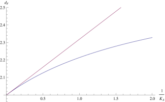
Figure 3: The fractal dimension $d_{F}$ as a function of $1/K_{A}$ for $D=3$. The upper curve is the leading order term in $1/K_{A}$ while the lower curve is our estimate (18).

.5 Conclusions

In this paper we studied hexatic membranes using a geometrical approach based on the effective average action. The $O(2)$–model coupled to the fluid membrane has a non–trivial RG fixed–point where the membrane is crinkled and has fractal dimension depending on the hexatic stiffness and on the embedding dimension with values between two and three.

This example shows how matter coupled to fluctuating geometries can induce physically interesting phases through the generation of non–local invariants. The calculation of the present paper gives an example of the non–trivial role played by non–local terms in the effective action, showing that their influence can drastically change the phase structure of a given model. In this light, it is important to consider the influence of non–local terms in other models of fluctuating geometry, such as membranes in higher dimensions Codello:2012dx or quantum gravity Codello:2011js .

This work also opens the road to the study of matter–membranes systems by the methods of the effective average action and the relative exact flow equation. The question that naturally arises is how flat space universality classes of $O(N)$–models Codello:2012ec , other than $N=2$, are dressed by the geometrical fluctuations of the membrane. Are there infinitely many fixed–points in the $N=0,1$ cases? Does the Mermin-Wagner-Hohenberg theorem applies to the $N\geq 2$ cases? This, and the inclusion of topological excitations in the $N=2$ case, will be subject of further studies.

Acknowledgments

We would like to thank D. Mouhanna for stimulating discussions and the LPTMC for hospitality. The research of O.Z. is supported by the DFG within the Emmy-Noether program (Grant SA/1975 1-1).

Appendix A

We report here some details about the calculation of the contributions to the beta functions of $\kappa_{k}$ and $\bar{\kappa}_{k}$ induced by the Polyakov action:

$$I_{P}[g]=\int\sqrt{g}\,R\frac{1}{\Delta}R\,.$$ (19)

Since we are expanding the rhs of the flow equation (6) to order $K^{2}$ or $R$, it is enough to keep only contributions of order $R$ in the Hessian of the Polyakov action (19). The expansion is conveniently written as:

$$\delta^{2}I_{P}[g]=\left.2\int d^{2}x\sqrt{g}\,\delta R\,\frac{1}{\Delta}\,\delta R\;\right|_{\delta g_{\mu\nu}=h_{\mu\nu}}\qquad\qquad$$

$$+\left.2\int d^{2}x\sqrt{g}\,R\,\frac{1}{\Delta}\,\delta R\;\right|_{\delta g_{\mu\nu}=H_{\mu\nu}}+O(R^{2},RK^{2})\,,\quad$$ (20)

with $h_{\mu\nu}=-2\nu^{i}K_{\alpha\beta}^{i}$ the first variation of the metric and $H_{\mu\nu}=2(\partial_{\alpha}\nu^{i}\partial_{\beta}\nu^{i}+\nu^{i}\nu^{j}K_{\alpha}^{i\gamma}K_{\gamma\beta}^{j})$ the second. After the expansion is performed, we can set the background metric, and implicitly the embedding field, equal to the metric of the two dimensional sphere; in this way we make all derivatives of the curvatures vanish, but we will still be able to disentangle the operators $R$ and $K^{2}$. Using the variation $\delta R=g^{\mu\nu}\Delta\delta g_{\mu\nu}+\nabla^{\mu}\nabla^{\nu}\delta g_{\mu\nu}-\frac{1}{2}g^{\mu\nu}\delta g_{\mu\nu}R$ we find:

$$\int d^{2}x\sqrt{g}\,R\frac{1}{\Delta}\delta R = \int d^{2}x\sqrt{g}\,H_{\mu\nu}\left(Rg^{\mu\nu}+\nabla^{\mu}\nabla^{\nu}\frac{1}{\Delta}R\right)+O(R^{2},RK^{2})$$

$$= \int d^{2}x\sqrt{g}\frac{R}{2}\,\nu^{i}\Delta\nu^{i}+O(R^{2},RK^{2})$$

$$\int d^{2}x\sqrt{g}\,\delta R\frac{1}{\Delta}\delta R = \int d^{2}x\sqrt{g}\left(h\Delta h+2h\nabla^{\mu}\nabla^{\nu}h_{\mu\nu}+h_{\alpha\beta}\frac{1}{\Delta}\nabla^{\alpha}\nabla^{\beta}\nabla^{\mu}\nabla^{\nu}h_{\mu\nu}\right)+O(R^{2})$$ (21)

$$= \int d^{2}x\sqrt{g}\left(\frac{1}{2}K^{i}K^{j}+K_{\alpha\beta}^{i}K^{j\alpha\beta}\right)\nu^{i}\Delta\nu^{j}+O(R^{2})\,.$$

In (21) we made the substitutions:

$$\nabla^{\mu}\nabla^{\nu} \rightarrow \frac{1}{2}\nabla^{2}g^{\mu\nu}$$

$$\nabla^{\alpha}\nabla^{\beta}\nabla^{\mu}\nabla^{\nu} \rightarrow \frac{1}{8}\nabla^{4}\left(g^{\alpha\beta}g^{\mu\nu}+g^{\alpha\mu}g^{\beta\nu}+g^{\alpha\nu}g^{\beta\mu}\right)\,,$$

that are allowed, to this order, under the trace in the flow equation and we used the relation $K_{\alpha\beta}K^{\alpha\beta}=K^{2}-R$ to simplify the first term. Inserting (21) in (20) gives the contribution (10) of the Polyakov action (19) to the Hessian (9) of the effective average action.

References

- (1) D. Nelson, T. Piran and S. Weinberg, Statistical mechanics of membranes and surfaces; M.J. Bowick and A. Travesset, Phys. Rept. (2001) 255, arXiv:cond-mat/0002038; D. Nelson, Defects and Geometry in Condensed Matter, Cambridge Univ. Press.
- (2) F. David, E. Guitter and L. Peliti, Journal de Physique (1987) 2059–2066.
- (3) D. Nelson, L. Peliti, Journal de Physique (1987) 1085–1092.
- (4) E. Guitter and M. Kardar, Europhys. Lett. 13 (1990) 441.
- (5) J. Berges, N. Tetradis and C. Wetterich, Phys. Rept. 363 (2002) 223, hep-ph/0005122.
- (6) A. Codello and O. Zanusso, Phys. Rev. D (2011) 125021, arXiv:1103.1089.
- (7) J.M. Kosterlitz and D.J. Thouless, J. Phys. C 6 (1973) 1181.
- (8) A.M.Polyakov, Phys. Lett. B103 (1981) 207-210.
- (9) M. Grater and C. Wetterich, Phys. Rev. Lett. 75 (1995) 378, hep-ph/9409459.
- (10) A. Codello, Annals Phys. (2010) 1727, arXiv:1004.2171.
- (11) J.P. Kownacki and D. Mouhanna, Phys. Rev. E (2009) 040101, arXiv:0811.0884; K. Essafi, J.-P. Kownacki and D. Mouhanna, Phys. Rev. Lett. (2011) 128102, arXiv:1011.6173.
- (12) A. Codello and R. Percacci, Phys. Lett. B 672 (2009) 280, arXiv:0810.0715.
- (13) J. Park and T. Lubensky, Phys. Rev. E (1996) 2648; J. Park and T. Lubensky, Phys. Rev. E (1996) 2665.
- (14) A. Codello, D. Mouhanna and O. Zanusso, in preparation.
- (15) D. Förster, Phys. Lett. A (1986) 115; H. Kleinert, Phys. Lett. B (1986) 335; A.M. Polyakov, Nucl. Phys. B (1986) 406.
- (16) E. Witten, Commun. Math. Phys. 92 (1984) 455.
- (17) N. D. Mermin and H. Wagner . Phys. Rev. Lett. 17(22) (1966) 1133; P. C. Hohenberg, Phys. Rev. 158(2) (1967); Coleman, S. (1973) Comm. Math. Phys. 264 (30819) 259.
- (18) A. Codello, N. Tetradis and O. Zanusso, JHEP 1304 (2013) 036, arXiv:1212.4073.
- (19) A. Codello, New J. Phys. 14 (2012) 015009 arXiv:1108.1908.
- (20) A. Codello and G. D’Odorico, Phys. Rev. Lett. 110 (2013) 141601 arXiv:1210.4037; A. Codello, J. Phys. A 45 (2012) 465006 arXiv:1204.3877.