Critical behaviour of the $XY$-rotors model on regular and small world networks

Abstract

We study the $XY$-rotors model on small networks whose number of links scales with the system size $N_{links}\sim N^{\gamma}$, where $1\leq\gamma\leq 2$. We first focus on regular one dimensional rings in the microcanonical ensemble. For $\gamma<1.5$ the model behaves like short-range one and no phase transition occurs. For $\gamma>1.5$, the system equilibrium properties are found to be identical to the mean field, which displays a second order phase transition at a critical energy density $\varepsilon=E/N,~{}\varepsilon_{c}=0.75$. Moreover for $\gamma_{c}\simeq 1.5$ we find that a non trivial state emerges, characterized by an infinite susceptibility. We then consider small world networks, using the Watts-Strogatz mechanism on the regular networks parametrized by $\gamma$. We first analyze the topology and find that the small world regime appears for rewiring probabilities which scale as $p_{SW}\propto 1/N^{\gamma}$. Then considering the $XY$-rotors model on these networks, we find that a second order phase transition occurs at a critical energy $\varepsilon_{c}$ which logarithmically depends on the topological parameters $p$ and $\gamma$. We also define a critical probability $p_{MF}$, corresponding to the probability beyond which the mean field is quantitatively recovered, and we analyze its dependence on $\gamma$.

I Introduction

Real-life networks are of finite size, loopy and display heavy correlations. This complexity represents a challenge from several points of view: first it is computationally expensive when attempting to investigate the network topology and to simulate dynamical systems upon it; moreover it becomes rapidly intractable analytically and one is obliged to make assumptions in order to simplify the picture and perform calculations. If this effort is crucial to practically afford problems, it also embeds a deeper question: facing the network complexity and their omnipresence in real world, it is fundamental to make the distinction between the essential variables which are able to catch the topology main features and those details which are unessential for a minimal though complete description. One of those very fruitful simplifications is sparseness, i.e. the networks considered have in general a few links per vertex while the network size tends to infinity. More precisely, a network is sparse if $k/N\rightarrow 0$ when $N\rightarrow\infty$, $k$ being the average degree. This basic hypothesis leads to a crucial consequence: locally, the network can be approximated by a tree, which means the absence of finite loops, i.e. finite closed paths, among the vertices. Sparseness and the local tree-likeness proved essential to analytical studies of dynamical systems on networks: we cite, focusing just on small-world networks, studies on the Ising model Viana Lopes et al. (2004); Herrero (2002), percolation Newman and Watts (1999) and, more recently, on the Kuramoto model (for a more complete overview, see Dorogovtsev et al. (2008)). Therefore, the advantage in terms of numerical computation is evident: in general, both numerical studies investigating the network topology Barrat and Weigt (2000); Newman et al. (2000) and critical phenomena on networks Viana Lopes et al. (2004); Herrero (2002); Kim et al. (2001); Medvedyeva et al. (2003) exploit the assumption of sparseness in its strongest form, taking the degree as constant. Nevertheless, increasing the links density, networks exist which are still sparse, fulfilling the aforementioned condition but they cannot no longer ensure the tree-likeness because of the heavy presence of loops. It could be argued hence that the links density could play a non negligible role both on the topological properties of those networks and on dynamical models defined upon them. Indeed it is the case of the $XY$-rotors model on regular one-dimensional chains: we show that the passage between a sparse network in the sense of $k=\mathcal{O}(1)$ and a dense one ($k=\mathcal{O}(N)$) implies the emergence of a new metastable state for which the thermodynamic order parameter does not relax at equilibrium De Nigris and Leoncini (2013). The links density hence triggers a non trivial effect on the thermodynamic behavior of the $XY$ model, which by itself is known for possessing a rich phenomenology investigated in several numerical studies Jain and Young (1986); Janke and Nather (1991); Kim (1994); Lee et al. (1984); Loft and DeGrand (1987); McCarthy (1986) on 2 and 3-D lattices. In particular, we would like to recall, as an example among many others, that the two dimensional case with nearest neighbors coupling is characterized by the famous Berezinskii-Kosterlitz-Thouless phase transition Kosterlitz and Thouless (1973); Leoncini et al. (1998), which implies the correlation function to switch from a power law decay at low temperatures to an exponential one in the high temperatures regime. In the mean field limit, the $XY$ model, called the Hamiltonian Mean Field (HFM) model in this case, displays as well a wide variety of behaviors this complexity being strongly entangled with the lack of additivity. Among its peculiarities we cite the presence of a second order phase transition of the magnetization Campa et al. (2009) and, even more noteworthy, the presence of non equilibrium quasi-stationary states of diverging duration in the thermodynamic limit Antoniazzi et al. (2007); Ettoumi and Firpo (2011); Latora et al. (2002); Chavanis et al. (2005); da C. Benetti et al. (2012); Pakter and Levin (2011). More recently, those models have been challenged to face more complex network topologies: for instance, studies exist concerning the HMF model on random graphs Ciani et al. (2011) where, varying the links density, a second order phase transition of the global magnetization is recovered for every density value in the thermodynamic limit. Furthermore, studies of the $XY$ model on small world networks Kim et al. (2001); Medvedyeva et al. (2003) proved that this lattice topology supports as well complex thermodynamical responses of the model: a mean field transition of the order parameter is retrieved and its critical energy seems to depend on the network parameters.
The present work inscribes itself on this line as we will focus, on first instance, on regular networks and then we will shuffle this regular topology with the introduction of a controlled amount of randomness. The first part of the paper being on regular networks, we detail the analytical calculations presented in De Nigris and Leoncini (2013) showing that tuning the link density allows to pass from a short-range regime to a long-range one. The analytical approach is preceded in Sec. III by the results of numerical simulations which are as well more extensively illustrated than in De Nigris and Leoncini (2013). Furthermore, we show that it exists between those two regimes a peculiar metastable state characterized by huge fluctuations of the order parameter. We then address, in the second part of the paper, small-world networks using the Watts-Strogatz model Watts and Strogatz (1998) aiming to shed light on the interplay between the link density and the injection of randomness in the network. In his regime we first investigate, acting on the links density $\gamma$ and on the rewiring probability $p$, the crossover from the regular lattice to the small-network topology. In Sec.IV.2 we consider the dynamics of the $XY$-rotors model on small-world networks and we show how the emergence of global coherence, via a mean field phase transition of the order parameter, strongly depends on the topological conditions fixed by $p$ and $\gamma$. Furthermore, we discuss in the last part how this influence turns out to be quantitative, affecting the critical energy $\varepsilon_{c}$ at which the phase transition occurs.

II The $XY$-Rotors Model

The $XY$-rotors model describes a set of $N$ spins interacting pairwise: each spin is fixed on the sites of a one dimensional ring and it is assigned with two canonically conjugated variables $\{\theta_{i},p_{i}\}$, $\theta_{i}\in\left[-\pi;\pi\right]$ being a rotation angle. The $XY$ Hamiltonian reads Antoni and Ruffo (1995); Leoncini et al. (1998):

$$H=\sum_{i=1}^{N}\frac{p_{i}^{2}}{2}+\frac{J}{2k}\sum_{i,j}^{N}a_{i,j}(1-\cos(\theta_{i}-\theta_{j})),$$ (1)

where $a_{i,j}$ is the matrix encoding the spins connections:

$$a_{i,j}=\begin{cases}1\,\,\mbox{if\,i$\neq$ j\ and\ are\, connected}\\ 0\,\,\mbox{otherwise}\end{cases}.$$ (2)

We take $J>0$, so that we are in the ferromagnetic case and in the following $J=1$ as well as the lattice spacing. Finally the $1/k$ factor in Eq. (1) ensures that the energy is an extensive quantity. $k$ is referred to as the degree and, to control the density of links in the network, we define it as:

$$k=\frac{2^{2-\gamma}(N-1)^{\gamma}}{N}\sim 2^{2-\gamma}N^{\gamma-1}.$$ (3)

Practically, we take the integer part of Eq. (3) since, once fixed $\gamma$ and $N$, $k$ is in general non integer. Since we assign $k$ links per spin and we set periodic boundary conditions, the system is translationally invariant. The dynamics are given by the set of Hamilton equations:

$$\dot{\theta_{i}} = \frac{\partial H}{\partial p_{i}}=p_{i},$$ (4)

$$\dot{p_{i}} = -\frac{\partial H}{\partial\theta_{i}}=-\frac{J}{k}\sum_{j\in V_{i}}^{N}\sin\left(\theta_{i}-\theta_{j}\right)$$

where $V_{i}$, represents the neighbors of rotor $i$. A global parameter, the magnetization is defined by

$$\mathbf{M} =\frac{1}{N} \left(\begin{array}[]{cc}&\sum\cos\theta_{i}\\ &\sum\sin\theta_{i}\end{array}\right)=M\left(\begin{array}[]{cc}\cos\varphi\\ \sin\varphi\end{array}\right)$$ (9)

in order to have an insight on the macroscopic behavior: we expect finite values of $M$ to indicate the emergence of a coherent inhomogeneous state , while a vanishing magnetization signals the absence of long-range order. We first study the response of the total equilibrium magnetization $M$ to the change of the underlying network via the $\gamma$ parameter. Practically, for each $\gamma$, we perform simulations within the microcanonical ensemble, by direct numerical integration of Eqs. (4) with the fifth order optimal symplectic integrator described in McLachlan and Atela (1992). The initial conditions of angles and momenta are picked from a Gaussian distributions with identical variance (which corresponds to a low temperature setting) and, to check the numerical integration, we monitor the conservation of the two constants of motion preserved by the dynamics: the energy $E=H$ and the total angular momentum $P=\sum_{i}p_{i}$, which we have set without loss of generality to $P=0$. Finally the time step is $\Delta t=0.05$ and we average the thermodynamic quantities over time only when the system has reached the equilibrium.

III Thermodynamic Behavior on Regular Lattices

III.1 : Numerical Computation

The regular network that we take into account is a one-dimensional chain of $N$ spins (rotors) with periodic boundary conditions for which each spin is connected to its $k$ nearest neighbors. By tuning the parameter $\gamma$, $1<\gamma\leq 2$ we act on the links density of the network. For $\gamma=1\,\,(k=2)$ the spins are connected to their nearest neighbors, while for $\gamma=2\,\,(k=N-1)$ the network is fully coupled. Heuristically, changing the value of $\gamma$ corresponds to change the range of interaction of each spin. Then two limit behaviors naturally emerge from this approach: the first is $\gamma\rightarrow$1 in which we expect the system to behave progressively like a one dimensional short range system with the existence of a continuous symmetry group, and so without any phase transition . On the other side, the $\gamma\rightarrow 2$ limit leads to the mean field regime and we expect the HMF transition of the magnetization to appear above a specific threshold of degree. We find this boundary value for $\gamma=1.5$ so that the two aforementioned limits translate more precisely in two intervals $\gamma<1.5$ and $\gamma>1.5$. Practically, for each $\gamma$ value, we monitor the average magnetization $\overline{M(N,\varepsilon)}$ (the bar indicates the temporal mean) for different sizes $N$ and for every energy density $\varepsilon=E/N$ in the physical range. The temporal mean is computed on the second half on the simulations: we start with the Gaussian initial conditions described in Sec. II and we simulate the dynamics, calculating the magnetization at each time step. When the system reaches a stationary state for the magnetization, we take the temporal mean as the equilibrium value.

We start our analysis with the $\gamma<1.5$ interval. The simulations are displayed

(a)
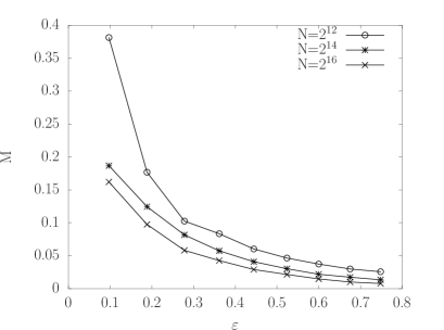
(b)

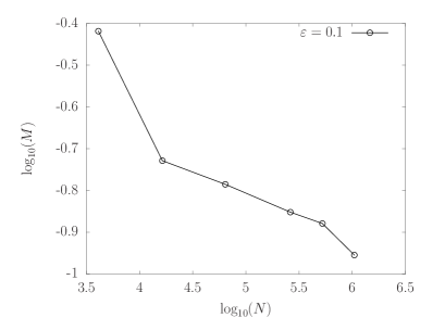
Figure 1: (a) Equilibrium magnetization versus energy density for $\gamma=1.25$ and different sizes. The error bars are of the size of the dots; (b) Residual magnetization for $\gamma=1.25$ at $\varepsilon=0.1$ versus the system size.

in Figs. 1a-b and as mentioned the magnetization smoothly vanishes with the energy (Fig. 1a). We have to recall that for low energies, the magnetization can be non-zero as a finite size effect, so the results displayed should depend on the system size. This is confirmed in Fig. 1, where the trend for the magnetization to vanish with increasing the size is exhibited. To check with even larger sizes, we consider in Fig. 1b the magnetization for a small energy density $\varepsilon=0.1$ and several sizes. The results clearly point out that the magnetization vanishes in the thermodynamic limit. When looking at relaxation scales, we found that larger sizes took more time to relax to equilibrium. So typically in our simulations we take as final time $t_{f}=20000$ for sizes up to $N=2^{16}$ and for $N>2^{18}$  $t_{f}=30000$.

Given these numerical results, we conclude that in the $\gamma<1.5$ interval, the system is short-ranged and the Mermin-Wagner theorem applies imposing the order parameter to vanish. Nevertheless, if long-range order is not possible, quasi long-range could still entail an infinite order phase transition of the correlation function, like in the two dimensional $XY$ model with nearest neighbors interactions. We recall that this particular type of critical phenomenon, first detected by Berezinskii, Kosterlitz and Thouless Kosterlitz and Thouless (1973), is characterized by two different types of decay of the correlation function with distance: a power law or an exponential decay, respectively for low and high temperatures. In order to look for such possibility we computed the correlation function

$$c(j)=\frac{1}{N}\sum_{i=1}^{N}\cos(\theta_{i}-\theta_{i+j\left[N\right]})\>,$$

for every $\varepsilon$ in the considered range. The results shown in Fig. 2

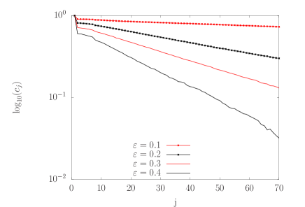
Figure 2: (color online) Correlation function $c_{j}$ for $\gamma=1.25$ and $N=2^{14}$.

indicate that the decay behavior is also exponential for low energies, demonstrating the absence of the aforementioned phase transition. This could have been anticipated from the fact that finite size effects on the magnetization even though present were small, but possible tricky effects of the boundary conditions could come into play, so it was worthwhile checking.

To summarize our result, we can conclude that, for $\gamma<1.5$, the spin degree is still too low for the system to show long-range or quasi long-range. Interestingly, the short range behavior is still at play even for configurations like $\gamma=1.4$ where each spin is under the influence of quite an important neighborhood since $k\propto N^{0.4}$ in this case.

Taking now in account the symmetric interval $\gamma>1.5$, the spins are connected enough to allow a coherent state to emerge: in Fig. 3

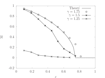
Figure 3: Equilibrium magnetization for $N=2^{16}$ and different $\gamma$. For $\gamma\neq 1.5$ the error bars are of the size of the dots.

the magnetization undergoes a second order phase transition at $\varepsilon_{c}=0.75$ which is well described by the HMF analytical curve. Again, around the delicate zone of the phase transition, finite size effects induce a shift between the theoretical prediction of the HMF and the simulations, but they can be smoothed down increasing the size. We recall that this phenomenon is also present for the full coupling $\gamma=2$. As a consequence we then find that even with a degree remarkably inferior (e.g. for $\gamma=1.6$ ) than the full coupling condition, each spin possesses enough connections to trigger the global behavior of the system and give a finite magnetization (at low energies). Of course, in both the intervals $\gamma\lessgtr 1.5$, the equilibrium magnetization is still affected by fluctuations because of the finite size effects. To monitor these we measured the magnetization variance $\sigma^{2}=\overline{(M-\overline{M})^{2}}$ and we show in Fig. 4 that it scales with the system size like

$$\sigma^{2}\propto 1/N.$$ (10)

This scaling is the one expected for the equilibrium state thus confirming that the values in Figs. 1a- 3 are representative of such state.

(a)

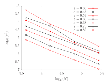
(b)

Figure 4: (color online) Scaling of the magnetization variance $\left\langle\sigma^{2}\right\rangle$ with the size for $\gamma=1.75$ (a) and $\gamma=1.5$ (b).

Given the results presented in the previous discussions, a natural critical value appears, which characterizes the shift from the short range picture to the long range one: $\gamma_{c}\simeq 1.5$. We decided to investigate the system behavior at this critical threshold imposing $\gamma=\gamma_{c}$. In fine, we expect that the system will be in a peculiar state by itself which cannot be labeled as short or long ranged. Results are depicted in Fig. 3. We observe that for low energies, $0.3\lesssim\varepsilon\leq 0.75$, the averaged magnetization is finite even when increasing the size but it remains lower than the mean field value. The effect is clearer when we look at its temporal behavior. It is indeed totally different than in the other two regimes and the order parameter $M$ shows large fluctuations which are orders of magnitude larger than for the other $\gamma$ regimes. We show in Fig. 5 a comparison a time series for the same energy and system size and different values of $\gamma$, namely $\gamma=1.75$ which displays a finite magnetization with small fluctuations and the one $\gamma=1.5$, with large fluctuations. In order to control the fact that these fluctuations are not an artifact of our initial conditions and that it is likely that the system does not relax on larger timescales than the previous configurations, we considered computation times up to a final time $t_{f}=200000$. Results are presented in Fig. 5, where it appears that this regime with large fluctuations persists. We recall that for $\gamma\lessgtr 1.5$ the simulation time was at most $t_{f}=30000$ and it was enough to reach a stationary state. Proceeding further, we notice that the amplitude of these fluctuations is not dependent on system size. We compare for instance $N=2^{12}$ to $N=2^{18}$ in Fig. 5 c and we conclude that for the aforementioned energies there is no significant amplitude decrease with system size. More precisely,

(a)
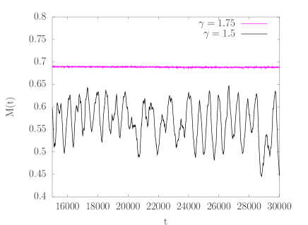
(b)
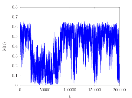
(c)
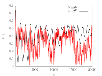
(d)

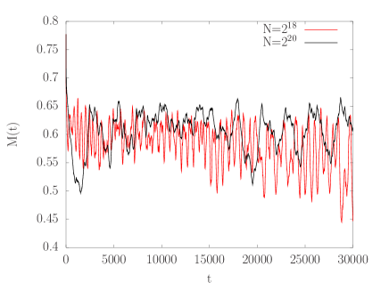
Figure 5: (color online) Time series for the magnetization with (a) $N=2^{18}$, $\varepsilon=0.60$; (b) $N=2^{12}$; $\varepsilon=0.44$; $T_{f}=200000$; (c) Comparison of the fluctuations amplitude of $N=2^{12}$ and $N=2^{18}$ with $\varepsilon=0.52$ and (d) of $N=2^{18}$ and $N=2^{20}$ with $\varepsilon=0.44$.

if we consider the variance $\sigma^{2}$ as before, it appears that the scaling of the variance mentioned in Eq. (10) and coherent with in the $\gamma\neq 1.5$ regimes, is substituted by a flat behavior increasing $N$ (see the results in Fig. 4b). It is worth noticing that the influence the system size can be retrieved not in the fluctuations amplitude but in the typical fluctuation time scale. In Figs. 5c-d, it becomes obvious that fluctuations appear to slow down with the system size. This time-scale dependence on the size is reminiscent of out of equilibrium behavior in systems with long range interactions, namely the lifetime of the Quasi Stationary States (QSS) Chavanis et al. (2008); Van Den Berg et al. (2010); Ettoumi and Firpo (2011, 2013) and further investigations are ongoing to shed light on this effect and on its potential analogy with the HMF results.

Heuristically, for $\gamma=\gamma_{c}$ it is like the if each spin does not possess enough connections to create a global order and establish the mean field but, nevertheless, the degree is sufficiently high ($\gamma=1.5$ corresponds to $k=\sqrt{N}$) to avoid the vanishing of the order parameter in the thermodynamic limit. The resulting behavior is reminiscent of a bistable regime oscillating between the $M=0$ configuration and the mean field value, which corresponds to a finite magnetization, we thus may expect some kind of intermittent behavior. In fine, the flatness of the variance suggests moreover that we observe a state with infinite susceptibility $\chi$ considering its canonical definition

$$\chi\sim\lim_{N\rightarrow\infty}N\sigma^{2}.$$ (11)

To conclude our analysis in symmetry with the $\gamma\lessgtr 1.5$ cases, we looked for a signature of this non trivial state in the correlation function but the fluctuations heavily affect it too so that it oscillates without showing a proper scaling.

III.2 Analytical Calculation

The numerical investigations illustrated point out that the degree triggers the shift from the pure one dimensional topology to the mean field frame. We now tackle this issue analytically aiming to retrieve the influence of the topology, encoded in the adjacency matrix $a_{i,j}$ (Eq. (2)), in the thermodynamic properties. We thus compute the magnetization in the low energy regime and check if the correct behavior is recovered, namely a zero magnetization for $\gamma<1.5$ and a finite value for $\gamma>1.5$. At low energies we have a clear separation between the magnetization values, with $M=0$ and the mean field one, in which as $\varepsilon\rightarrow 0\,\,M\rightarrow 1$. In this limit, due to the ferromagnetic coupling it is natural to assume the differences $\theta_{i}-\theta_{j}$ are small when $a_{i,j}=1$ so that the connected spins are mostly aligned in order to minimize the free energy. We can hence develop the Hamiltonian at the leading order:

$$H=\sum_{i}\frac{p_{i}^{2}}{2}+\frac{J}{4k}\sum_{i,j}a_{i,j}(\theta_{i}-\theta_{j})^{2}\>,$$ (12)

so that our system reduces to a collection of oscillators connected by $a_{i,j}$. We then choose to represent the spin field as a superposition of modes, following the recipe given in refs Leoncini et al. (1998); Leoncini and Verga (2001):

$$\begin{array}[]{c}\theta_{i}=\sum_{l=0}^{N-1}\alpha_{l}(t)\cos(\frac{2\pi li}{N}+\phi_{l})\\ p_{i}=\sum_{l=0}^{N-1}\dot{\alpha_{l}}(t)\cos(\frac{2\pi li}{N}+\phi_{l})\end{array}.$$ (13)

In Eq. (13), we sum over $N$ modes so that the change of variables is linear and we observe that, given the periodic boundary conditions, it just corresponds to perform a discrete Fourier transform. The amplitudes $\alpha_{l}$ are, in our approach, the information carriers of the temporal behavior, hence the representation of the momenta $p_{i}$ is related to the one of the angles via the first Hamilton equation $p_{i}=\dot{\theta_{i}}$. The phases $\phi_{l}$ are randomly distributed on the circle to ensure that the momenta $p_{i}$ are Gaussian distributed in the limit $N\rightarrow\infty$ as theoretically predicted for the microcanonical ensemble. Following the approach described in Leoncini and Verga (2001), if we consider different sets of phases $\{\phi_{l}\}_{m}$ labeled by $m$ we can interpret each set as a realization of the system, i.e. a trajectory in the phase space. Hence the process of averaging on random phases would correspond to ensemble averaging and leads to dynamic equations which, nevertheless, embed information about the thermodynamic state of the system, via the phase averaging. If we now inject Eq. (13) in the Hamiltonian (12) we obtain for the kinetic part $K$:

$$\frac{\left\langle K\right\rangle}{N}=\frac{1}{N}\left\langle\sum_{i}\frac{p_{i}^{2}}{2}\right\rangle=\frac{1}{4}\sum_{l}\dot{\alpha}_{l}^{2},$$ (14)

where $\left\langle...\right\rangle$ stands for the average over random phases. In Eq. (14) we used the relation:

$$\left\langle\cos(k_{i}+\phi_{i})cos(k_{j}+\phi_{j})\right\rangle=\frac{1}{2}\delta_{i,j}.$$

For the potential, we have that the adjacency matrix $a_{i,j}$ is a circulant one because of the definition of the regular network given in Sec. II which is translationally invariant. Hence we can diagonalize it, obtaining a real spectrum $\{\lambda_{j}\}$ since $a_{i,j}$ is a real symmetric matrix. The spectrum analytical expression in general reads:

$$\lambda_{j}=\frac{1}{k}\sum_{l=1}^{N-1}c_{l}e^{\frac{2\pi ijl}{N}},$$ (15)

where the vector $c_{l}$ is the coefficient vector whose permutations compose the matrix $a_{i,j}$. Because of the two symmetries $c_{l}=c_{N-l}$ and $e^{\frac{2\pi ij(N-l)}{N}}=e^{\frac{-2\pi ilj}{N}}$, Eq. (15) can be splitted in two sums:

$$\lambda_{j}=\frac{1}{k}\left(\sum_{l=1}^{\frac{N}{2}}c_{l}e^{\frac{2\pi ijl}{N}}+\sum_{l=1}^{\frac{N}{2}}c_{l}e^{\frac{-2\pi ijl}{N}}\right),$$ (16)

which can hence be written as the sum of the real parts:

$$\lambda_{j}=\frac{2}{k}\sum_{l=1}^{k/2}\cos(\frac{2\pi lj}{N})=\frac{1}{k}\left[\frac{\sin[(k+1)j\pi/N]}{\sin(j\pi/N)}-1\right],$$ (17)

where $k$ is the spin degree of Eq. (3). To the leading order the potential will hence take the form:

$$\frac{V}{N}=\frac{1}{4kN}\sum_{i,j}a_{i,j}(\theta_{i}-\theta_{j})^{2}=\frac{1}{2}\sum_{l}(1-\lambda_{l})\left|\hat{\theta_{l}}\right|^{2}$$ (18)

In Eq. (18) we used the identity

$$\frac{1}{kN}\sum_{i,j}a_{i,j}\theta_{i}\theta_{j}=\frac{1}{kN}\Theta^{T}P^{*}DP\Theta=\sum_{l}\lambda_{l}\left|\hat{\theta_{l}}\right|^{2},$$ (19)

where $\Theta=\left(\theta_{1}...\theta_{N}\right)$ and $a_{i,j}=P^{*}DP$. In the latter equation $D$ is the diagonal form of the adiacency matrix and $P^{-1}=P^{*}$ since $P$ is unitary. The identity in Eq. (19) comes from the fact that the eigenvectors of a circulant matrix of size $N$ are the columns of the unitary discrete Fourier transform matrix of the same size. We can then inject in Eq. (18) the linear waves representation and average over the phases as we did for the kinetic part of the Hamiltonian:

$$\frac{\left\langle V\right\rangle}{N}=\left\langle\frac{1}{2}\sum_{l}(1-\lambda_{l})\left|\hat{\theta_{l}}\right|^{2}\right\rangle=\frac{1}{4}\sum_{l}(1-\lambda_{l})\alpha_{l}^{2}.$$

Having obtained the averaged Hamiltonian $\left\langle H\right\rangle=\left\langle K\right\rangle+\left\langle V\right\rangle$, we can deduce the averaged equation of motion, as anticipated, via the second Hamilton equation

$$\frac{d}{dt}\left(\frac{\partial\left\langle H\right\rangle}{\partial\dot{\alpha_{l}}}\right)=-\frac{\partial\left\langle H\right\rangle}{\partial\alpha_{l}}\>,$$

and obtain

$$\ddot{\alpha_{l}}=-(1-\lambda_{l})\alpha_{l}=-\omega_{l}^{2}\alpha_{l}.$$ (20)

We have hence an equation for an harmonic oscillator whose frequency depends on the adjacency matrix spectrum and, consequently, on the spin degree. We note that this approach is dependent from our low temperatures approximation, but as mentioned we shall make use of this since, depending on the value of $\gamma$, we expect two clearly defined regimes of zero or finite magnetization. Our system is now completely encoded in terms of wave amplitudes $\{\alpha_{l}\}$ and frequencies $\{\omega_{l}\}$ which can be linked observing that, at equilibrium, we have the equipartition of the modes ($p_{i}$’s are Gaussian):

$$T=\frac{1}{N}\sum_{i}\left\langle p_{i}^{2}\right\rangle=\frac{1}{2}\sum_{l}\alpha_{l}^{2}\omega_{l}^{2}\Rightarrow\alpha_{l}^{2}=\frac{2T}{N(1-\lambda_{l})}.$$

In order to compute $M$, we apply the same procedure, meaning that we average over the phases its expression given by Eq. (9) after having substituted the representation Eq. (13). We obtain Leoncini et al. (1998):

$$\left\langle\mathbf{M}\right\rangle=\prod_{l}J_{0}(\alpha_{l})(\cos\theta_{0},\sin\theta_{0}),$$ (21)

where $J_{0}$ is the zeroth order Bessel function and $\theta_{0}$ is the average of the angles $\{\theta_{i}\}$, $\theta_{0}=\frac{1}{N}\sum_{i}{\theta_{i}}$. This quantity is conserved because of the translational invariance, giving a constant total momentum $P$ which is set at $P=0$ by our choice of initial conditions. As the final step to evaluate Eq. (21), we recall that we are dealing with a low temperatures approximation so we can consider that the amplitudes $\alpha_{l}^{2}$ to be small at equilibrium and in the large system size limit Leoncini and Verga (2001). This consideration allows to develop at leading order the product of the Bessel functions and, taking the logarithm of Eq. (21), we finally obtain:

$$\ln\left(\left\langle M\right\rangle\right)=-\sum_{l}\frac{\alpha_{l}^{2}}{4}=-\frac{T}{2N}\sum_{l}\frac{1}{1-\lambda_{l}}.$$ (22)

Eq. (22) conjugates the thermodynamic information and the topological one because of the matrix spectrum. If, from one side, it actually realizes our purpose of matching these two levels of description, now the spectrum in Eq. (17) carries the system complexity, requiring Eq. (22) to be evaluated numerically. In Fig. 6

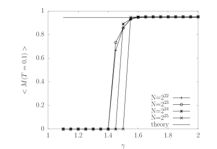
Figure 6: Analytical magnetization $\left\langle M\right\rangle$ from Eq. (22) for $T=0.1$ versus $\gamma$. Theory refers to the exact analytical solution of the HMF model.

we show, increasing the size, how this approximated expression grasps the correct asymptotic behavior, giving the mean field value in the high $\gamma$ regime and vanishing for low $\gamma$. The transition becomes sharper at $\gamma_{c}\simeq 1.5$ by increasing the size and gives hence confirmation of its critical signification as already pointed out by our numerical simulations of Sec.III.

IV The Small World Network Model

In Secs. III.1-III.2 we considered a regular chain as network topology and we illustrated how the degree drives the thermodynamic response of the $XY$-model on those lattices from the short-range regime to the long-range one. The natural following step to reorganize the topology is now to break the translational invariance of the regular chain previously considered and to introduce some randomness in how the spins are connected. In this purpose, we used the Watts-Strogatz model (W-S)Watts and Strogatz (1998) for small-world networks, which interpolates between a regular network and a random one by the progressive introduction of random long-range connections. Following the algorithm devised in Watts and Strogatz (1998), each link is reconnected with probability $p$ to a randomly chosen other vertex or is left untouched with probability $1-p$: long-range connections are hence introduced and the rewiring procedure injects disorder in the network since $k,$ fixed by Eq. (3) at the beginning, is non-uniform afterwards. The degree distribution decays exponentially since the rewiring is performed independently for every vertex Barrat and Weigt (2000). Moreover, since $k_{i}\approx\left\langle k\right\rangle$, a W-S network is not locally equivalent, even in the limit case of $p=1$, to a random graph were eventually isolated vertex exist and the network is fragmented in many parts Barrat and Weigt (2000). It is noteworthy for the following to add that the rewiring injects mainly shortcuts whose length is of the order of the network size $\mathcal{O\left(N\right)},$ so that a fine tuning of the interaction range by the means of the randomness $p$ is not possible.

IV.1 Network analysis

The small-world regime embeds characteristics of both the regular lattice and the random network ones: the network keeps track of the initial configuration since, after the rewiring, it still conserves a local neighborhood like a regular lattice; on the other hand the network approaches, in the sense specified in Sec. IV, the random graph topology because of the shortcuts induced by the rewiring. In our context it hence emerges naturally the question of how the degree, which scales as $k\sim N^{\gamma-1}$, could influence the scaling of topological quantities in competition with the rewiring probability $p$. For instance, a crucial passage in which the $\gamma$ parameter could play an important role is the crossover from the regular chain topology to the small-world regime. It is usually investigated by the scaling behavior of the average path length $l(p,\gamma)$, defined as the average shortest distance between spins.

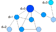
Figure 7: (color online) Path lengths starting from the blue vertex.

This quantity has an algebraic increase $l\sim N$ for a regular one-dimensional lattice with fixed degree $k$, while for random networks it grows as $l\sim\log N$. The passage between those two regimes is enhanced by the long-range connections which could allow the spins to behave coherently. Practically, since the network lacks a metric, the distance between two spins is calculated as the minimal number of edges to cross to go from one spin to the other, as shown in Fig. 7. To investigate the change between these two behaviors we perform numerical simulations, varying $\gamma$ and $p$: we use values for $\gamma$ from 1.2 to 1.5 and $p$ ranges from $10^{-7}$ up to $10^{-3}$ . $N$ is fixed at $2^{14}$ and we average over 10 network realizations for each value of $p$. In Fig. 8a we plot $l(\gamma,p)/l(\gamma,0)$ versus $\gamma$. $l(\gamma,p)$ shows the known crossover behavior Watts and Strogatz (1998) but, considering the probability $p_{SW}(N,p,\gamma)$ at which $l(\gamma,p)$ drops abruptly to the random network values, it appears evident that it is strongly dependent on $\gamma$. We have the following scaling for $p_{SW}(N,\gamma)$ Newman and Watts (1999), using the degree definition in Eq. (3):

$$p_{SW}\sim\frac{1}{N^{D}kD}\propto\left(\frac{1}{N}\right)^{\gamma},$$ (23)

where $D=1$ is the dimension of the initial regular lattice. In Fig. 8b we plot the estimation of $p_{SW}(N,\gamma)$ from the simulations versus $\gamma$ which effectively confirm the power law of Eq. (23). The degree is hence crucial to quantitatively determine the passage to the small-world regime; this dependence unveils its importance considering that, on small-world networks, a ”topological” length scale can be defined Newman and Watts (1999) as

$$\xi=1/(pkD)^{1/D}$$ (24)

and then $p_{SW}$ in Eq. (23) is the probability of having $\xi=N$ . This is the key condition to achieve global coherence and it clearly appears that the density of links, governed by the parameter $\gamma$, and the randomness injected by $p$ concur in complexifying the network topology. In Sec. III, we then move one step further dealing with the thermodynamics of the $XY$-rotors model on the small-world network and looking for the topological signature of the $\gamma$ and $p$ parameters in its properties.

(a)
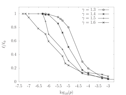
(b)
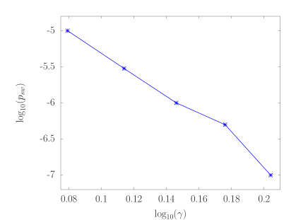
(c)
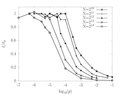
(d)

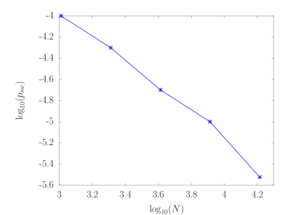
Figure 8: (a) Average path lengths versus rewiring probability for different $\gamma$ values and $N=2^{14}$. (b) Power law scaling of $p_{SW}(\gamma)$. (c) Average path lengths versus rewiring probability for different $N$ values and $\gamma=1.3$ . (d) Power law scaling of $p_{SW}(\gamma=1.3)$. The curve slope is $\approx 1.27$, coherent with the scaling in Eq. (23).

IV.2 Thermodynamic Behavior on Small World Networks

In Sec. IV.1 we focused on the topological interplay of $\gamma$ and $p$ parameters in establishing the small-world regime which, as explained, is noteworthy for its ambivalence, resembling both to a regular lattice and to a random graph. In this section we put the $XY$-rotors model on a small-world network: the question we address now is to investigate the thermodynamic counterpart of the network complex topology. We focus the low $\gamma$ regime, i.e. $\gamma<1.5$. In this case we recall that the degree is still too low to induce long-range order by itself without the intervention of randomness and the network behaves like a one-dimensional chain. In the interval $\gamma>1.5$ the high degree already induces a mean field phase transition of the magnetization whose critical energy is $\varepsilon_{c}=0.75$, as shown in Sec. III. In this interval, even without the contribution of long-range connections, the network is connected enough to behave like a full-coupled one, which is the case of the Hamiltonian Mean Field model. On the other hand, in the case of random networks, it has been shown that the mean field phase transition appears for all $\gamma>1$ Ciani et al. (2011). We thus introduce progressively long-range connections with the rewiring probability $p$ since, from Eq. (24), we expect to retrieve two regimes determined by $\gamma$ and $p$; $\xi>N$ in which long-range order is absent and $\xi<N$ where the order parameter displays a second order phase transition.

(a)

(b)

(c)

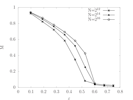
Figure 9: Average magnetization $M$ versus energy density $\varepsilon=E/N$ for several system sizes, $\gamma=1.25$ and $p=0.001\,\,(a),\,0.005\,\,(b),\,0.05\,\,(c).$

In Figs. 9a-c we set $\gamma=1.25$ and, for each value of $p$, we consider several system sizes, above and below the threshold $\xi(1.25,p,N)=N$. The results displayed in Figs. 9 show the equilibrium mean value of the magnetization $\overline{M}$ versus the energy density $\varepsilon=E/N$: for $N=2^{12}$, the probabilities $p=0.001$ and $0.005$ (Figs. 9 a-b) are still too low to entail the crossover to the long-range regime and the system does not undergo a phase transition. On the other hand, the other two sizes considered $N=2^{14}$ and $2^{16}$ are in the $\xi<N$ regime and the mean field phase transition is recovered all the $p$ taken in account. As explained, increasing the randomness decreases the small-world threshold; hence all the sizes show the phase transition of the magnetization for $p=0.05$ (Fig. 9c). Those results suggest the importance of $\xi$ also from the statistical point of view: in Sec. IV.1, we showed that it signals the topological passage from regular to small-world network which identifies itself by a drop of the average path distance $l(N,\gamma,p)$; equivalently in this short $l(N,\gamma,p)$ regime the existence of long-range order is possible and, thus, we observe the second field phase transition of the thermodynamic order parameter. Remarkably, the critical energy $\varepsilon_{c}$ at which the transition occurs varies accordingly to the randomness; we thus investigate this effect tuning $\gamma$ between $1.2$ and $1.5$ and $p$ from $10^{-7}$ to $10^{-3}$. As explained before, it is worth focusing on the interval $\gamma\leq 1.5$. In this case the shortcuts introduced by the rewiring process are crucial for the achievement of global coherence; while in the $\gamma>1.5$ we already know that phase transition with $\varepsilon_{c}=\varepsilon_{HMF}=0.75$ occurs both on regular chains De Nigris and Leoncini (2013) and on random networks Ciani et al. (2011).

(a)
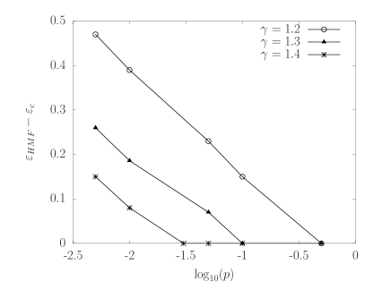
(b)
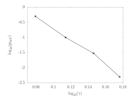
(c)

Figure 10: (a) Logarithmic dependence of the critical energy $\varepsilon_{c}$ versus the rewiring probability $p$ for different $\gamma$ values. (b) Power law scaling of $p_{MF}(\gamma)$. (c) Phase plot in the $\left(\gamma,p\right)$ plane. The thick line for $p=0$ and $1<\gamma$<1.5 stands for the absence of phase transitions in that parameter region. In the “$MF$ phase transition“ region, the critical energy is the same of $HMF$, $\varepsilon_{c}=0.75$.

In Fig. 10, we plot the critical energy $\varepsilon_{c}(p,\gamma)$ versus the rewiring probability $p$ for several values of $\gamma$ and we observe that the phase boundary seems to be well described by the logarithmic form :

$$\varepsilon_{c}=\log(g(\gamma)p^{c})$$ (25)

with $C\sim 0.1$. Eq. (25) is coherent with the scaling proposed in Kim et al. (2001); Medvedyeva et al. (2003) as far as the $p$ dependence is concerned. Remarkably, in Kim et al. (2001); Medvedyeva et al. (2003), it was a result issued from Monte-Carlo simulations in the canonical ensemble while we work in the microcanonical frame. Moreover the aforementioned results of logarithmic scaling were found in the $p\rightarrow 0$ regime, while where we are exploring regions with large values of $p$. We also have to insist on the fact that Eq. (25) embeds an extra piece of information concerning the degree. Indeed, in our analysis the “quantitative” topological parameter $\gamma$ affects in his turn the critical energy $\varepsilon_{c}$ through the function $g(\gamma)$ , showing the non trivial role played by the links density in the thermodynamic behavior of the $XY$-rotors model.

Another specific information can be retrieved from Fig. 10a. There is a threshold beyond which a “saturation” process exists: to be more explicit, for each value of $\gamma$, we define a threshold probability $p_{MF}(\gamma)$ for which the critical energy is $\varepsilon_{c}=0.75$, identical to values obtained in the mean field ($\gamma=2$), or for the fully randomized networks Ciani et al. (2011). For $p>p_{MF}(\gamma)$ increasing the randomness does not influence anymore the critical energy and in some way the resulting small-world network is, from the thermodynamic point of view, equivalent to a fully coupled graph. In Fig. 10b, we show how this probability threshold $p_{MF}(\gamma)$ depends as a power law on the $\gamma$ parameter. Note though that we expect that $p_{MF}\rightarrow 0$ when $\gamma\rightarrow 1.5$, because as we discussed before in the $\gamma>1.5$ regime the system is already in the mean field state without any rewiring. Regarding Fig. 10b, we do not expect the results to be valid near $\gamma=1.5$. Indeed a precise estimation of $p_{MF}$ proves to be very delicate since it relies in its turn on the determination of the critical energy of the transition which is intrinsically a hard task. Moreover the simulations are performed with finite size systems, so the measured $p_{MF}$ is influenced by finite size effects. Then we actually have $p_{MF}(\gamma,N)$ and this dependence on $N$ can entail a finite value even for $\gamma=1.5$. We also have to mention that we average on a finite number of network realizations, which may affect as well the results. An interesting path to follow in order to avoid this effects and refine our estimations could be the use of finite-size scaling techniques. Moreover, since previous results exist in the canonical ensemble Medvedyeva et al. (2003); Kim et al. (2001), this analysis would be of interest in our approach because we deal with the microcanonical ensemble. It would then be possible to compare the characteristics of the phase transition in the two ensembles and shed light on their equivalence. Proceeding in our analysis, we recall that for the regular network a metastable state was found for $\gamma_{c}\simeq 1.5$ in which the order parameter is affected by heavy fluctuations, suggesting that the system oscillates between low magnetization values, proper of the $\gamma<1.5$ regime, and the mean field value of the $\gamma>1.5$ case. We can notice that, after the introduction of randomness, we do not observe this metastable state for $\gamma=1.5$ or any other value of $\gamma$. In fact now a small (eventually vanishing) $p$ is enough to generate a phase transition. It therefore exists an interplay between the “quantitative” parameter $\gamma$ and the “qualitative” parameter $p$; nevertheless those parameters, as anticipated in Sec. IV, are not equivalent when dealing with their influence on the thermodynamic behavior of the $XY$-model. This duality is so far not complete since it was not possible to retrieve the metastable state in the $\gamma<1.5$ regime acting exclusively on the $p$ parameter. In this sense, the randomness is “regularizing” the thermodynamic behavior: the rewired network supports either the behavior of a regular lattice either, once the small-world regime is reached, gives rise to the phase transition of the magnetization. Summarizing, we can say that the noise created by the rewiring stabilizes the passage between the two regimes and destroys the delicate metastable state which arose in the regular lattice.

V Conclusion

In conclusion, we have studied the influence on the critical behavior of the $XY$-rotors model of two different network topologies, the regular lattice and small world network. In Sec. III, we introduced the parameter $\gamma$ which allows to tune the number of links from the linear chain to the full coupling configuration. We identified two main parameter regions: the first for $\gamma<1.5$ in which the model has a one dimensional behavior and thus it does not display long-range or quasi long-range order as shown by numerical simulations. On the contrary, in the second region $(\gamma>1.5)$, the spin degree is sufficiently high to lead to the emergence of a coherent state: we thus observe a mean field phase transition of the magnetization, identical to the one of the HMF model. More interestingly, we show numerical and analytical evidence of an unstable state at the threshold between the two regions, for $\gamma_{c}\simeq 1.5$. In this peculiar state, the magnetization is affected by fluctuations which seem to be size independent and, furthermore, this state does not reach equilibrium on the timescales considered. We then calculated analytically an approximated expression for the magnetization, obtained in the low temperatures regime, which demonstrates the topological critical nature of $\gamma_{c}\simeq 1.5$. This expression retrieves correctly the two behaviors aforementioned and, since it contains the spectrum of the adjacency matrix, it points out that the topological origin of the three different phases shown by the simulations. We have then studied the role of the links density on the topology of small-world networks and its effect on the $XY$-rotors model dynamics. We have focused, in Sec. IV, on the crossover to the small-world regime tuning the $\gamma$ parameter. We show by numerical simulations that $p_{SW}$ has the scaling in Eq. (23) which is therefore consistent with Newman and Watts (1999). Hence the links density, governed by $\gamma$, turns out to be crucial to enhance the crossover between the “large-world” regime and the small-world one cooperating with the rewiring probability $p$ in the creation of long-range connections. We then investigated, in Sec. IV.2, the thermodynamic response of the $XY$-rotors model to the variations of the network underlying. We retrieved the emergence of a mean field transition of the magnetization once $p>p_{SW}$. This latter condition implies the network to be in the $\xi<N$ case, using the definition in Eq. (24), implying that the passage between the regular and the small-world topology also entails a difference in the behaviour of the model. Moreover we found a logarithmic dependence of the critical energy $\varepsilon_{c}(p,\gamma)$ on $p$ and $\gamma$ which lead to the scaling in Eq. (10). The interplay between the topological parameters in modifying $\varepsilon_{c}$ saturates when $\varepsilon_{c}=0.75$ which is the critical energy of the Hamiltonian Field model and we defined a new threshold probability $p_{MF}$ which displays the power law scaling with $\gamma$ shown in Fig. 10b. We hence found that a small (vanishing) amount of randomness regularizes the $\gamma=1.5$ metastable state pointed out in Sec. III and moreover it was not possible to recreate it in the $\gamma<1.5$ interval just adding long-range connections with $p$. Therefore, as far as the thermodynamic behavior is concerned, we conclude that $\gamma$ and $p$ are not equivalent when dealing with the transition to the mean field state; nevertheless, we anticipate here that a more refined criteria than randomness could be found in order to perturb the regular network in the low density regime $(\gamma<1.5)$ and enhance the creation of out-of-equilibrium effects like the $\gamma_{c}\simeq 1.5$ metastable state.