Ponderomotive modification of multicomponent magnetospheric plasma due to electromagnetic ion cyclotron waves

A. K. Nekrasov* and F. Z. Feygin**

Abstract We derive the expression for the ponderomotive force in the real multicomponent magnetospheric plasma containing heavy ions. The ponderomotive force considered includes the induced magnetic moment of all the species and arises due to inhomogeneity of the traveling low-frequency electromagnetic wave amplitude in the nonuniform medium. The nonlinear stationary force balance equation is obtained taking into account the gravitational and centrifugal forces for the plasma consisting of the electrons, protons and heavy ions (He⁺). The background geomagnetic field is taken for the dayside of the magnetosphere, where the magnetic field have magnetic ”holes” (Antonova and Shabansky 1968). The balance equation is solved numerically to obtain the nonlinear density distribution of ions (H⁺) in the presence of heavy ions (He⁺). It is shown that for frequencies less than the helium gyrofrequency at the equator the nonlinear plasma density perturbations are peaked in the vicinity of the equator due to the action of the ponderomotive force. A comparison of the cases of the dipole and dayside magnetosphere is provided. It is obtained that the presence of heavy ions leads to decrease of the proton density modification.

Keywords Earth · Magnetic fields · Plasmas · Ponderomotive force · Waves

1 Introduction

A considerable attention has been paid to study an influence of heavy ions (mainly helium and oxygen) on the generation and dynamics of electromagnetic ion cyclotron (EMIC) waves in the frequency range 0.5 to 5.0 Hz traveling along the geomagnetic field lines. Using the searchcoil magnetometer and particle spectrometer data on board of the GEOS 1 and ATS 6 satellites, Young et al. (1981), Mauk et al. (1981) and Fraser et al. (1982) came to the conclusion that EMIC waves are strongly controlled by the dynamics of heavy ions. Later on, Kozyra et al. (1984) and Fraser et al. (1992) obtained similar results, using the ISEE 1 and 2 data.

The propagation of the EMIC waves along magnetic field lines in a heavy ion rich plasma is characterized by the reverse of polarization and the splitting of the wave spectrum into two branches, the high-frequency branch $\omega>\omega_{ch}$ ($\omega$ is the wave frequency, $\omega_{ch}$ is the heavy ion gyrofrequency) and the low-frequency branch $\omega<\omega_{ch}$. The two branches are separated by a stop-band. Observations on board of the GEOS 1 and 2 satellites (Young et al. 1981) have shown that the EMIC wave spectra are concentrated in the vicinity of the equatorial He⁺ gyrofrequency. These observations also showed that there is an inverse connection between the increase of the He⁺ concentration and the appearance of the Pc1 events on the ground that confirms the important role of the He⁺ ions for the generation and propagation of the EMIC waves.

As is well-known, ponderomotive forces induced by the EMIC waves contribute to the plasma balance in the Earth’s magnetosphere (e.g. Allan 1992; Guglielmi et al. 1993, 1995; Guglielmi and Pokhotelov 1994; Witt et al. 1995; Pokhotelov et al. 1996; Allan and Manuel 1996; Feygin et al. 1998; Nekrasov and Feygin 2011, 2012). In studies mentioned above, the magnetosphere has been assumed to contain only one ion species (H⁺). In this paper, we explore the effect of the ponderomotive force in the real multicomponent magnetospheric plasma. In the numerical analysis, the plasma consisting of the electrons, protons and heavy ions (He⁺) is considered. The background geomagnetic field is taken for the dayside of the magnetosphere, where the magnetic field have magnetic ”holes” (Antonova and Shabansky 1968). The stationary nonlinear balance equation is solved numerically to obtain the nonlinear density distribution of ions (H⁺) in the presence of heavy ions (He⁺). Without heavy ions, this problem has been treated by Nekrasov and Feygin (2012).

The paper is organized as follows. In Sect. 2, we describe the geomagnetic field model of the dayside magnetosphere. The ponderomotive force in the multicomponent plasma is derived in Sect. 3. The stationary force balance equation is considered in Sect. 4. In Sect. 5, the results of numerical calculations of the balance equation for the nonlinear plasma modification in the curvature geomagnetic field are represented. Conclusive remarks and discussion are given in Sect. 6.

2 Geomagnetic field model of the dayside magnetosphere

We here apply a model of the Earth’s magnetic field given by Antonova and Shabansky (1968). This model has been shown to be in a good agreement with magnetic field observations by the HEOS 1 and 2 satellites in the dayside magnetosphere (Antonova et al. 1983). According to this model, the geomagnetic field is described by a superposition of two dipoles: the internal dipole with the magnetic moment $M$ and the additional external dipole with the magnetic moment $kM$ ($k$ is a constant parameter) disposed at the distance $a$ (measured in the units of the Earth’s radius $R_{E}$) on the dayside of the magnetosphere along the Earth-Sun line from the position of the original dipole. The latter dipole models the distortion of the geomagnetic field caused by the solar wind pressure. The model by Antonova and Shabansky (1968) is sufficiently simple and convenient for an analysis of geophysical phenomena in the dayside magnetosphere. We have described this model in our paper Nekrasov and Feygin (2012). However, for convenience of reading, we also give the main moments here.

In the spherical coordinate system, magnetic field components for the two-dipole model by Antonova and Shabansky (1968) in the meridional noon-midnight plane have the form

$$B_{r}=-\frac{2B_{E}x}{r^{3}}\alpha,$$ (1)

$$B_{\varphi}=\frac{B_{E}}{r^{3}}\sqrt{1-x^{2}}\beta,$$ (2)

where $x=\sin\varphi$, $\varphi$ is the geomagnetic latitude, $r$ is measured in the units $R_{E}$, and $B_{E}$ $=0.311$ G is the equatorial magnetic field at the Earth’s surface. Coefficients $\alpha$ and $\beta$ are the following:

$$\ \alpha=1-\frac{kr^{3}\left(a^{2}-2r^{2}+ar\sqrt{1-x^{2}}\right)}{2\left(a^{2}+r^{2}-2ar\sqrt{1-x^{2}}\right)^{5/2}},$$ (3)

$$\ \ \beta=1+\frac{kr^{3}\left[\sqrt{1-x^{2}}\left(a^{2}+r^{2}\right)-ar\left(2+x^{2}\right)\right]}{\sqrt{1-x^{2}}\left(a^{2}+r^{2}-2ar\sqrt{1-x^{2}}\right)^{5/2}}.$$ (4)

The total magnetic field $B$ in an arbitrary point of the field line can be defined from (1) and (2) as

$$B=\frac{B_{E}}{r^{3}}\left[4x^{2}\alpha^{2}+\left(1-x^{2}\right)\beta^{2}\right]^{1/2}.$$ (5)

An equation for the field line is determined by $dr/rd\varphi=B_{r}/B_{\varphi}$ or

$$\frac{dr}{dx}=-\frac{2xr}{1-x^{2}}\frac{\alpha}{\beta}.$$ (6)

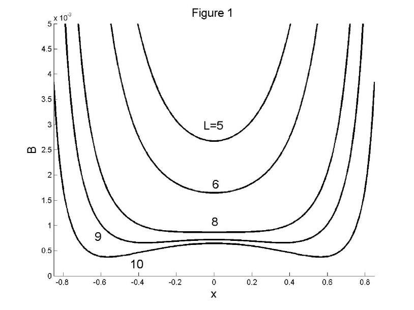
Figure 1: The dependence of the Earth’s magnetic field $B$ (in G) on the geomagnetic latitude $\varphi$ in the meridional plane of the dayside magnetosphere for different $L$ in the model by Antonova and Shabansky (1968)

The magnetic field $B$ described by (5) has along the near boundary field lines two minima located symmetrically relative to the equator (Antonova and Shabansky 1968). When $a$ tends to infinity, the values $\alpha$ and $\beta$ tend to $1$ (see 3 and 4). In this case, we have a transition to the one-dipole approximation. The dependence of the geomagnetic field (5) on $x$ for different distances from the Earth is shown in Fig. 1, where $L$ is the McIlwain parameter.

3 Ponderomotive force in the multicomponent plasma

3.1 Ponderomotive force due to the longitudinal inhomogeneity of the wave amplitude

To find the ponderomotive force of electromagnetic waves in the multicomponent plasma, we use the results of the paper by Nekrasov and Feygin (2006). The equation for the nonlinear slow velocity $\left\langle\mathbf{v}_{j2}\right\rangle$ is given by

$$\frac{\partial\left\langle\mathbf{v}_{j2}\right\rangle}{\partial t}=\frac{q_{j}}{m_{j}}\left(\left\langle\mathbf{E}_{2}\right\rangle+\left\langle\mathbf{F}_{j2}\right\rangle\right),$$ (7)

where $q_{j}$ and $m_{j}$ are the charge and mass of the species $j$, $\left\langle\mathbf{E}_{2}\right\rangle$ is the slow nonlinear electric field, $\left\langle\mathbf{F}_{j2}\right\rangle$ is equal to

$$\left\langle\mathbf{F}_{j2}\right\rangle=-\frac{m_{j}}{q_{j}}\left\langle\mathbf{v}_{j1}\cdot\mathbf{\nabla v}_{j1}\right\rangle+\frac{1}{c}\left\langle\mathbf{v}_{j1}\times\mathbf{B}_{1}\right\rangle,$$ (8)

the angle brackets $\left\langle{}\right\rangle$ denote the time-averaging over fast oscillations. The subscript $1$ in (8) relates to the linear perturbations of the velocity, $\mathbf{v}_{j1}$, and magnetic field, $\mathbf{B}_{1}$.

We are interested in the nonlinear motion of a plasma along the background magnetic field. We assume that the latter has the $\mathbf{z}$-direction. In the case of the EMIC waves also traveling along the magnetic field, the equation (7) for the longitudinal velocity $\left\langle v_{j2z}\right\rangle$ takes the form

$$\frac{\partial\left\langle v_{j2z}\right\rangle}{\partial t}=-\frac{q_{j}}{m_{j}}\frac{1}{\omega_{pe}^{2}}\sum_{l}\omega_{pl}^{2}\left(\left\langle F_{l2z}\right\rangle-\left\langle F_{j2z}\right\rangle\right)$$ (9)

and the value $\left\langle F_{j2z}\right\rangle$ defined by (8) is given by

$$\left\langle F_{j2z}\right\rangle=-\frac{q_{j}}{2m_{j}}\frac{1}{\sigma\omega\left(\sigma\omega-\omega_{cj}\right)}\frac{\partial\left\langle\mathbf{E}_{1}^{2}\right\rangle}{\partial z},$$ (10)

where $\omega>0$ is the wave frequency, $\sigma=\pm 1$ denotes the left ($+$) or right ($-$) polarization of the wave, $\omega_{pj}=\left(4\pi n_{j}q_{j}^{2}/m_{j}\right)^{1/2}$ is the plasma frequency, $n_{j}$ is the background number density, $\omega_{cj}=q_{j}B/m_{j}c$ is the cyclotron frequency, $c$ is the speed of light in vacuum and $\mathbf{E}_{1}=\operatorname{Re}\mathbf{E}_{10}\exp\left(i\int^{z}kdz-i\omega t\right)$ is the wave electric field with the nonuniform amplitude. When obtaining (9) and (10), we have used (11)-(13), (16) and (17) in Nekrasov and Feygin (2006), have taken into account that $v_{j1z}=0$ for waves under consideration and have assumed that $\partial/\partial z\gg k\partial/\omega\partial t$, where $\partial/\partial t$ is applied to the wave amplitude. The right-hand side of (9) (without $m_{j}$) is the particular (see below) ponderomotive force acting on species $j$.

Using (9), we can define the total particular ponderomotive force in the multicomponent plasma as

$$F_{p1z}=\sum_{j}m_{j}n_{j}\frac{\partial\left\langle v_{j2z}\right\rangle}{\partial t}=-\frac{1}{\omega_{pe}^{2}}\sum_{j,l}q_{j}n_{j}\omega_{pl}^{2}\left(\left\langle F_{l2z}\right\rangle-\left\langle F_{j2z}\right\rangle\right).$$ (11)

Taking into account (10), the expression (11) gets the following:

$$F_{p1z}=-\frac{1}{8\pi}\sum_{j\neq e}\frac{\omega_{pj}^{2}}{\omega_{cj}\left(\sigma\omega-\omega_{cj}\right)}\frac{\partial\left\langle\mathbf{E}_{1}^{2}\right\rangle}{\partial z},$$ (12)

where we have neglected small terms proportional to $m_{e}$, which describe the ponderomotive force acting on the electrons.

3.2 Ponderomotive force due to the transverse inhomogeneity of the wave amplitude. Magnetic moment

It is known that if the medium has the own magnetic moment (magnetic field) $\mathbf{M}$ and is embedded in the external nonuniform magnetic field $\mathbf{B}$, then this medium is subjected by the action of the force

$$\mathbf{F}_{\mathbf{M}}=\left(\mathbf{M\cdot\nabla}\right)\mathbf{B}$$ (13)

(see e.g. Landau and Lifshits 1982). The EMIC waves propagating along the geomagnetic field generate the nonlinear magnetic field that can be found from (3), (16) and (17) in (Nekrasov and Feygin 2006). Neglecting in (16) (Nekrasov and Feygin 2006) small terms and passing to the space-time representation, we find the equation for the transverse nonlinear electric field $\left\langle E_{2x}\right\rangle$

$$\left(\mathbf{\nabla}^{2}c_{A}^{2}-\frac{\partial^{2}}{\partial t^{2}}\right)\left\langle E_{2x}\right\rangle=\frac{c_{A}^{2}}{c^{2}}\frac{\partial^{2}}{\partial t^{2}}\left\langle C_{x}\right\rangle,$$ (14)

where $\mathbf{\nabla}^{2}=\partial^{2}/\partial y^{2}+\partial^{2}/\partial z^{2}$, $c^{2}/c_{A}^{2}=\sum_{j}\omega_{pj}^{2}/\omega_{cj}^{2}$, $c_{A}$ is the Alfvén velocity and

$$\frac{\partial\left\langle C_{x}\right\rangle}{\partial t}=-\frac{c}{2B}\sum_{j}\frac{\omega_{pj}^{2}}{\left(\sigma\omega-\omega_{cj}\right)^{2}}\frac{\partial\left\langle\mathbf{E}_{1}^{2}\right\rangle}{\partial y}$$ (15)

(see (17) in (Nekrasov and Feygin 2006)).

We further assume that $\partial^{2}/\partial y^{2}\gg\partial^{2}/\partial z^{2}$ and $c_{A}^{2}\partial^{2}/\partial y^{2}\gg\partial^{2}/\partial t^{2}$. Then from (14) and (15), we obtain

$$\frac{\partial\left\langle E_{2x}\right\rangle}{\partial y}=-\frac{1}{2cB}\sum_{j}\frac{\omega_{pj}^{2}}{\left(\sigma\omega-\omega_{cj}\right)^{2}}\frac{\partial\left\langle\mathbf{E}_{1}^{2}\right\rangle}{\partial t}.$$ (16)

From Faraday’s equation

$$\mathbf{\nabla\times}\left\langle\mathbf{E}_{2}\right\rangle=-\frac{1}{c}\frac{\partial\left\langle\mathbf{B}_{2}\right\rangle}{\partial t},$$ (17)

we can find the induced nonlinear magnetic field $\left\langle\mathbf{B}_{2}\right\rangle$. Substituting (17) into (16), we have in our case for the multicomponent plasma

$$\left\langle B_{2z}\right\rangle=-\frac{1}{2B}\sum_{j}\frac{\omega_{pj}^{2}}{\left(\sigma\omega-\omega_{cj}\right)^{2}}\left\langle\mathbf{E}_{1}^{2}\right\rangle.$$ (18)

We note that this expression for the two-component plasma (electrons and ions) has been derived by Nekrasov and Feygin (2005).

The magnetic moment $\mathbf{M}$ is connected with the induced magnetic field as $4\pi\mathbf{M=}\left\langle\mathbf{B}_{2}\right\rangle$. Using this relation, we obtain in our case the expression (13) for $\mathbf{F}_{\mathbf{M}}$ along the magnetic field

$$F_{\mathbf{M}z}=\frac{1}{4\pi}\left\langle B_{2z}\right\rangle\frac{\partial B}{\partial z}.$$ (19)

This expression for the two-component plasma has also been obtained by Nekrasov and Feygin (2005), but in a different way. However, we see here under which conditions (18) takes place.

3.3 Total ponderomotive force in the nonuniform medium

The total ponderomotive force $F_{pz}$ is equal to sum of (12) and (19)

$$F_{pz}=-\frac{1}{8\pi}\sum_{j\neq e}\frac{\omega_{pj}^{2}}{\omega_{cj}\left(\sigma\omega-\omega_{cj}\right)}\left[\frac{\partial\left\langle\mathbf{E}_{1}^{2}\right\rangle}{\partial z}+\frac{\omega_{cj}}{\left(\sigma\omega-\omega_{cj}\right)}\frac{\partial B}{B\partial z}\left\langle\mathbf{E}_{1}^{2}\right\rangle\right],$$ (20)

where we have neglected the contribution of the electrons into (18). We further assume that the wave amplitude depends on the $z$-coordinate because of the longitudinal medium inhomogeneity. In this case, the amplitude of the wave $E_{10}$ in the WKB-approximation is proportional to $N_{z}^{-1/2}$, where $N_{z}$ is the refractive index equal to

$$N_{z}^{2}=1-\sum_{j\neq e}\frac{\omega_{pj}^{2}}{\omega_{cj}\left(\sigma\omega-\omega_{cj}\right)}$$ (21)

(see e.g. (14) in (Nekrasov and Feygin 2006)). When obtaining (21), we have used the condition of quasineutrality $\sum_{j}q_{j}n_{j}=0$. We see that the first term in the square brackets in (20) can be written in the form

$$F_{p1z}=\frac{1}{8\pi}\left(N_{z}^{2}-1\right)\frac{\partial\left\langle\mathbf{E}_{1}^{2}\right\rangle}{\partial z}.$$

Calculating the value $\partial\left\langle\mathbf{E}_{1}^{2}\right\rangle/\partial z$ through $\partial N_{z}^{2}/\partial z$, using (21) and substituting the result into (20), we find

$$F_{pz}=-\frac{\left\langle\mathbf{E}_{1}^{2}\right\rangle}{16\pi}\sum_{j\neq e}\frac{\omega_{pj}^{2}}{\omega_{cj}\left(\omega_{cj}-\sigma\omega\right)}\left\{\frac{\partial\ln n_{j}}{\partial z}+\left[\frac{\sigma\omega}{\omega_{cj}-\sigma\omega}+\frac{2\omega_{cj}}{\left(\omega_{cj}-\sigma\omega\right)}\frac{1}{N_{z}^{2}}\right]\frac{\partial\ln B}{\partial z}\right\}.$$ (22)

Thus, the ponderomotive force in the multi-component plasma is the sum of the ponderomotive forces for each ion species.

4 Stationary force balance equation

From equations of motion for the species $j$ in the second approximation on the wave amplitude averaged over fast oscillations, we can obtain the force balance equation in the stationary state. The total equation of motion contains except the electromagnetic force also the gradient of thermal pressure, the gravity and centrifugal force (e.g. Lemaire 1989; Persoon et al. 2009).

We assume for simplicity that all the species have the equal temperatures $T_{j}=T=const$. Consider the three-component plasma consisting of the electrons ($e$), protons ($i$) and heavy ions ($h$). In the stationary case, adding the corresponding equations of motion for each species, we obtain for the nonlinear time-averaging density perturbations $n_{j2}$ the following force balance equation along the magnetic field line:

$$T\nabla_{\|}\left[2n_{i2}+\left(1+\frac{q_{h}}{q_{i}}\right)n_{h2}\right]=\left(m_{i}n_{i2}+m_{h}n_{h2}\right)\left(g_{\|}\mathbf{+}n_{\Omega\|}\Omega^{2}R_{E}r\cos\varphi\right)+F_{p\|},$$ (23)

where the subscript $\|$ denotes the local $\mathbf{z}$-direction. Here, we have used the condition of quasineutrality and the equality $q_{i}=-q_{e}$. In (23), the value $g_{\|}=\mathbf{g\cdot b=-}g_{E}B_{r}/r^{2}B$ is the longitudinal gravitational acceleration ($g_{E}=9.8$ m sec^-2), $\Omega$ is the Earth’s rotation frequency and $n_{\Omega\parallel}=\mathbf{n}_{\Omega}\cdot\mathbf{b}$, where $\mathbf{n}_{\Omega}$ and $\mathbf{b}$ are the unit vectors along the centrifugal force and magnetic field, respectively.The value $n_{\Omega\parallel}$ is equal to $n_{\Omega\parallel}=\left(1+\beta/2\alpha\right)\left(B_{r}/B\right)\cos\varphi$ (see Nekrasov and Feygin 2012). We note that in the last paper in (14) $\cos^{2}\varphi$ stands erroneously instead of $\cos\varphi$.

In (22), we will express the value $\left\langle\mathbf{E}_{1}^{2}\right\rangle$ through the amplitude of the wave magnetic field at the equator $B_{10}$. From Faraday’s equation, it is followed that $N_{z}^{2}\left\langle\mathbf{E}_{1}^{2}\right\rangle=\left\langle\mathbf{B}_{1}^{2}\right\rangle$, where $\left\langle\mathbf{E}_{1}^{2}\right\rangle\propto N_{z}^{-1}$. Thus, we obtain that $\left\langle\mathbf{E}_{1}^{2}\right\rangle=B_{10}^{2}\left(N_{z0}N_{z}\right)^{-1}$ for circularly-polarized waves. Here and below, the subscript $0$ relates to the values at the equator. The operator $\nabla_{\parallel}$ in (23) is defined by the relation $\nabla_{\parallel}=\mathbf{b}\cdot\mathbf{\nabla}$ and has been found in (Nekrasov and Feygin 2012)

$$\nabla_{\parallel}=2R_{E}^{-1}\eta^{-1/2}\frac{d}{dx},$$ (24)

where

$$\eta=\left(\frac{dr}{dx}\right)^{2}+\frac{r^{2}}{1-x^{2}}.$$ (25)

We further connect the perturbation $n_{h2}$ with $n_{i2}$. From the nonlinear continuity equation and equation of motion (9), we can obtain an estimation of this connection

$$n_{h2}\sim n_{i2}\frac{m_{i}}{m_{h}}\frac{H}{P}\frac{\left(1-\nu_{i0}\frac{B_{0}}{B}\right)}{\left(1-\nu_{h0}\frac{B_{0}}{B}\right)},$$ (26)

where $P=\rho_{i}/\rho_{i0},H=\rho_{h}/\rho_{i0},\rho_{i}=n_{i}m_{i},\rho_{h}=m_{h}n_{h},\nu_{i0}=\sigma\omega/\omega_{ci0},\nu_{h0}=\sigma\omega/\omega_{ch0}$.

For the three-component plasma, substituting (22), (24) and (26) into (23), we obtain the following equation:

$$\frac{d\delta}{dx}=\frac{1}{\lambda}\left(A_{1}-\frac{d\lambda}{dx}\right)\delta+\frac{1}{\lambda}A_{2}\left(A_{3}+A_{4}+A_{5}+A_{6}\right),$$ (27)

where $\delta=\rho_{i2}/\rho_{i0}$, $\rho_{i2}=m_{i}n_{i2}$ and

$$\lambda=2+\left(1+\frac{q_{h}}{q_{i}}\right)\frac{m_{i}}{m_{h}}\frac{H}{P}\frac{\left(1-\nu_{i0}\frac{B_{0}}{B}\right)}{\left(1-\nu_{h0}\frac{B_{0}}{B}\right)}.$$ (28)

In (27), we have introduced the notations

$$A_{1} =\frac{2R_{E}x\alpha\mu g_{eff}}{\left(1-x^{2}\right)\left|\beta\right|c_{si}^{2}r},$$ (29)

$$A_{2} =-\frac{B_{10}^{2}}{8\pi\rho_{i0}c_{si}^{2}}\frac{B_{0}}{B}\left(\frac{1}{\mu\mu_{0}}\right)^{1/2}\frac{\left(1-\nu_{i0}\right)^{1/2}}{\left(1-\nu_{i0}\frac{B_{0}}{B}\right)^{1/2}},$$

$$A_{3} =\frac{1}{P^{1/2}}\frac{dP}{dx},$$

$$A_{4} =\frac{\left(1-\nu_{i0}\frac{B_{0}}{B}\right)}{\left(1-\nu_{h0}\frac{B_{0}}{B}\right)}\frac{1}{P^{1/2}}\frac{dH}{dx},$$

$$A_{5} =P^{1/2}\frac{\left(\nu_{i0}\frac{B_{0}}{B}+\frac{2}{N_{z}^{2}}\right)}{\left(1-\nu_{i0}\frac{B_{0}}{B}\right)}\frac{1}{B}\frac{\partial B}{\partial x},$$

$$A_{6} =\frac{H}{P^{1/2}}\frac{\left(1-\nu_{i0}\frac{B_{0}}{B}\right)}{\left(1-\nu_{h0}\frac{B_{0}}{B}\right)^{2}}\left(\nu_{h0}\frac{B_{0}}{B}+\frac{2}{N_{z}^{2}}\right)\frac{1}{B}\frac{\partial B}{\partial x},$$

where $c_{si}^{2}=2T/m_{i}$ and

$$g_{eff}=g_{E}+g_{cf}=g_{E}-\left(1+\beta/2\alpha\right)\Omega^{2}R_{E}r^{3}\cos^{2}\varphi,$$ (30)

$$\mu =1+\frac{H}{P}\frac{\left(1-\nu_{i0}\frac{B_{0}}{B}\right)}{\left(1-\nu_{h0}\frac{B_{0}}{B}\right)},$$ (31)

$$N_{z}^{2} =4\pi c^{2}\frac{\rho_{i}}{B^{2}}\frac{1}{\left(1-\nu_{i0}\frac{B_{0}}{B}\right)}\mu.$$

We consider that $N_{z}^{2}\gg 1$. The value $\mu_{0}$ is obtained from (31) at $x=0$. When obtaining $A_{1}$, we have used (1), (5), (6) and (25).

For the equilibrium mass density of H⁺ ($i$) and He⁺ ($h$), we take the power law form to describe the longitudinal field line distribution, $\rho_{j}\propto r^{-\gamma}$, where $j=i,h$. For the large distances from the Earth’s surface which we consider below, the choice $\gamma=1$ is the best one to be appropriate to experimental data (Denton et al. 2006). Thus, we set

$$\rho_{j}\left(x\right)=\rho_{j0}\left(1-x^{2}\right)^{-1}.$$

This formula can be applied up to $\varphi\approx\pm 50-60^{0}$ (Denton et al. 2006). In this case, $P=\left(1-x^{2}\right)^{-1}$ and $H=H_{0}\left(1-x^{2}\right)^{-1}$. These values will be substituted to (28) and (29). We note that in our case $m_{h}=4m_{i}$.

5 Numerical analysis

Equation (27) for the two-component magnetospheric plasma has been analyzed in (Nekrasov and Feygin 2012) by the Runge-Kutta method, making use of the boundary condition $\delta=0.06$ at $\ x=0$. Thus, we have obtained effects of the action of the ponderomotive, gravitational and centrifugal forces on the plasma density distribution at $x\neq 0$, at the same time perturbations at the equator remained unchanged. In this paper, we set the boundary condition $\delta=0$ at $x=0.8$. This case permits us to consider the plasma density modification in the region of the equator. For numerical calculations, we have used the same parameters for the magnetic field model as that in (Nekrasov and Feygin 2012): $a=33$ and $k=13$ (except for Figs. 3a,b). These parameters correspond to the dayside boundary of the magnetosphere at the distance $10R_{E}$ obtained by HEOS 1 and 2 satellites (Antonova at al. 1983). Other parameters are the following: $c_{si}^{2}=10^{9}$ m² $\sec^{-2}$, $\rho_{i0}=1.67\times 10^{-20}$ kg m^-3 for all $L$ near the midday boundary of the Earth’s magnetosphere, where the plasma density depends weakly on $L$ (Chappel 1974; Carpenter and Anderson 1992). In all the numerical calculations, we have taken $\sigma=+1$ and assumed that $\nu_{h0}<1$ to avoid the singularity $1-\nu_{h}=0$. As heavy ions, we use He⁺.

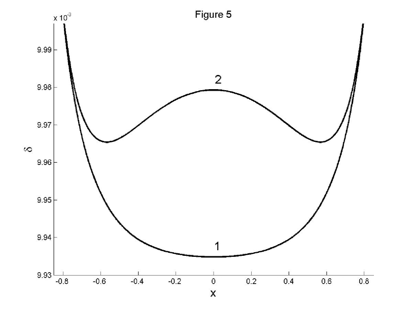
Figure 5: The dependence of $\delta$ on $x$ at $L=10$ and $B_{10}=0$ for $H_{0}=0.5$. The curve 1 corresponds to $\Omega=0$. The curve 2 - $g_{eff}\neq 0$.

Figures 2 depict the distribution of the normalized nonlinear proton density $\delta=\rho_{i2}/\rho_{i0}$ along the field line for different values of $H_{0}=0,0.5,1.0$ at $L=6,10$ for $B_{10}=10^{-5}$ G. We have set $\nu_{i0}=0.1$ to have $\nu_{h0}<1$. We see that the plasma density perturbation increases in the direction of the equator due to the action of the ponderomotive force (without the latter see Fig. 5). The equatorial value of $\delta$ decreases with increasing of $H_{0}$ because of increasing of $\lambda$ and $\mu$ with $H_{0}$ (see (27)-(29) and (31)).

Figures 3 represent a difference in the $\delta$-distribution for the dipole ($k=0$) and two-dipole ($k=13$) geomagnetic field at $L=8$ and $H_{0}=0,1.0$ for $B_{10}=10^{-5}$ G. We see that the peak value of $\delta$ at the equator is smaller for $k=13$ than for $k=0$. This can be explained by increasing of the equatorial geomagnetic field $B$ due to $k\neq 0$ (see (3)-(5)), which stands in the denominator of $A_{2}$ (see (29)) and decreases the ponderomotive force. The presence of heavy ions also results in a decreased influence of the ponderomotive force on the ions due to increase of the parameters $\lambda$ and $\mu$ (as in Fig. 2). Therefore, for $H_{0}=1.0$, the values of $\delta$ are smaller than for $H_{0}=0$. We note that the curves for $H_{0}=0.5$ are here and in Figs. 4 situated between the curves with $H_{0}=0,1.0$ (except Fig.5).

Figures 4 show the dependence of the relative density perturbation $\delta$ on $x$ for different values of the wave amplitude $B_{10}=(1,3,5)\times 10^{-5}$ G for $L=10$ and $H_{0}=0,1.0$. It can be seen that increased wave-amplitude yields increased values of $\delta$ along field lines. The smaller values of $\delta$ at $H_{0}=1.0$ are explained in the description of Figs. 2a, 2b and 3a, 3b.

Figure 5 describes formally the case $B_{10}=0$ to show the role of the gravitational and centrifugal forces (see (30)). It is followed from (27) that gravitational force increases the plasma density (not only perturbations!) with larger distances from the equator. This is shown by the curve 1. The centrifugal force has the opposite direction (see (30)) and drives a plasma to the equator. Far from equator, the gravitational force is larger than the centrifugal one (see also Sect. 6). In the vicinity of the equator, on the contrary, the centrifugal force is larger. This results in a peak of plasma density at the equator. The curve 2 shows the corresponding distribution. The equatorial values of $\delta$ for the curves 1 and 2 are decreasing with increasing $H_{0}$. The boundary condition for the curves 1 and 2 is $\delta=0.01$ at $x=0.8$ since to solve (27) for $A_{2}=0$ it is necessary to have a nonzero boundary condition for $\delta$.

All the figures demonstrate that the density perturbation is peaked at the equator due to ponderomotive and centrifugal forces. Such peaking is observed in the magnetosphere of the Earth (Denton et al. 2006).

6 Conclusion and Discussion

We conclude by summarizing main results obtained in this paper:

1). We have derived the general expression for the ponderomotive force induced by electromagnetic ion cyclotron waves in a multicomponent plasma containing different species of ions.

2). The correct equation of the force balance along the magnetic field lines, which contains the perturbed thermal plasma pressure together with the ponderomotive force, having the same (second) order of magnitude, has been considered.

3). We have investigated the effect of the ponderomotive force on the perturbed ion (proton) density distribution in the presence of helium ions.

4). It has been shown that for frequencies less than the helium gyrofrequency at the equator the nonlinear plasma density perturbations are peaked in the vicinity of the equator due to the action of the ponderomotive force. The maximum of the ion (proton) density perturbation has been obtained to decrease with increasing of the heavy ion (He⁺) mass density.

5). We have obtained that larger wave-amplitudes inducing more ponderomotive force result in larger $\delta$-perturbations.

Theoretical and numerical results given above in this section are the main points of our exploration. The derivation of expression for the ponderomotive force in the multicomponent plasma containing different species of heavy ions is particularly important. This permits us to consider the influence of wave perturbations on the redistrbution of magnetospheric plasma in the direction of the equator in conditions close to real ones. As we see, the equatorial value of the proton density distribution should drop for more abundance of He⁺.

We have considered the relative role of the gravitational and centrifugal forces when the wave activity is absent, $B_{10}=0$ (Fig. 5). We see from (30) that the gravitational and centrifugal forces along the magnetic field lines have opposite directions. At some latitude $\varphi_{eq}$, both forces are equal to each other. Taking into account (6), the estimation of $\varphi_{eq}$ for $\alpha\sim\beta\sim 1$ is the following:

$$\cos\varphi_{eq}\approx\left(\frac{2g_{E}}{3\Omega^{2}R_{E}r_{0}^{3}}\right)^{1/8},$$ (32)

where $r_{0}R_{E}$ is the equatorial distance of the given magnetic field line from the Earth’s center ($r_{0}=L$). At $\varphi>\varphi_{eq}$, the gravitational force is larger than the centrifugal one. When $\varphi<\varphi_{eq}$, the centrifugal force is dominant. For $r_{0}=8$, we obtain $\cos\varphi_{eq}\approx 0.89$ or $\varphi_{eq}\approx 27{{}^{\circ}}$. When $r_{0}=10$, we have $\cos\varphi_{eq}\approx 0.82$ and $\varphi_{eq}\approx 35{{}^{\circ}}$.

From (27), we can roughly estimate the relative contribution of the ponderomotive force $F_{p}$ and of the gravitational and centrifugal forces $F_{g+c}$ as

$$\frac{F_{p}}{F_{g+c}}\sim\frac{A_{2}A_{3}}{A_{1}\delta}.$$ (33)

Assuming that $\delta$-perturbation is due to the wave action, we estimate in our case $\delta\sim A_{2}$. Substitution of $\delta$ in (33) gives

$$\frac{F_{p}}{F_{g+c}}\sim\frac{A_{3}}{A_{1}}\approx\frac{c_{si}^{2}r_{0}}{R_{E}g_{E}}.$$

For $r_{0}=10$ and $c_{si}^{2}=10^{9}$ m² $\sec^{-2}$, we find $F_{p}/F_{g+c}\sim 160$. We see that the ponderomotive force is dominant because $A_{1}\ll 1$ (for $x\lesssim 1$). We note that a change of the boundary condition by the nonzero valus of $\delta$ in Fig. 2b does not influence on the form of the curves. Thus, we can expect substantial increases in $\delta$-perturbations during more geomagnetically active periods (Figs. 4a, 4b). This result is qualitatively consistent with observational data, such as Denton et al. (2006), which show a larger equatorial mass density peak with larger wave amplitudes (see their Figure 12). As a possible reason for this effect, Denton et al. (2006) indicate a role of the ponderomotive force in driving ions up the field line.

We have investigated the nonlinear plasma density redistribution for the Antonova and Shabansky (1968) model of the geomagnetic field $B$ given in Fig. 1. This choice is justified by its sufficient simplicity. In addition, the model by Antonova and Shabansky (1968) provides a complete analytical description of the geomagnetic field on the dayside of the Earth’s magnetosphere and is in accordance with satellite measurements. The use of a more complex geometry for $B$ such as T96 (Tsyganenko 1995) could be justified for taking into account some details (the local time, position, the solar wind parameters etc.). However, the results obtained will qualitatively remain the same because the main form of the magnetic field lines does not essentially change.

In this paper, we have applied the theory of perturbations to obtain the ponderomotive force expression and the force balance equation. We assumed that $n_{j2}\ll n_{j0}$. The value $\delta$ for parameters used is in the region $\delta\sim 2\times 10^{-3}\div 6\times 10^{-2}$ (see Figs. 2-4). Thus, perturbations are small in comparison with the background density. During active wave periods, density perturbations can be of the same order of magnitude as background values (see Denton et al. 2006). Therefore, there is some problem to compare theoretical  and experimental results. However, for the limiting estimation, we could take such wave amplitudes, for which $\delta\sim 1$, where $\delta\sim\left|A_{2}\right|$. For $\rho_{i0}$ and $c_{si}^{2}$ given in Sect. 5 and $H_{0}=1$, we obtain roughly $B_{10}\sim 10^{-4}$ G.

We have derived the ponderomotive force for circularly-polarized waves traveling along the magnetic field. For example, in papers by Denton et al. (2004, 2006) and Takahashi et al. (2006), toroidal Alfvén waves were discussed. Therefore, it is worth to derive ponderomotive forces for other types of perturbations. The case of the strong nonlinearity when density perturbations are the same as background values deserves also to be examined.

We have assumed that condition of quasineutrality is satisfied in the background and perturbation states. It is followed, for example, from the paper by Denton et al. (2006), that equatorial peaking is observed for ions and absent for electrons. We think that a large electric field should arise in this case.

It is obvious that for a detailed comparison of theoretical results with observational data, theoretical models should be adequate to real experimental conditions and observations and vice versa. It is important to be sure that a stationary symmetric theoretical picture considered here is relevant to real situations. The equatorial peaking in this picture is possible, if the wave action is symmetric and simultaneous from both ionospheric boundaries to the equator during some time for establishment of the stationary state and wave amplitudes should decrease from the ionosphere to the equator. In other cases, dynamical (nonstationary) processes can play a role.

Acknowledgements We gratefully thank the anonymous referee for his/her very constructive and useful comments which have helped considerably to improve a presentation of this paper. We also acknowledge the financial support from the Russian Foundation for Basic Research, research grants No. 11-05-00920 and the Program of Russian Academy of Sciences No. 22 and 4.

References

Allan, W.: J. Geophys. Res. 97, 8483 (1992)

Allan, W., Manuel, J. R.: Ann. Geophys. 14, 893 (1996)

Antonova, A.E., Shabansky, V.P.: Geomagn. Aeron. 8, 639 (1968)

Antonova, A.E., Shabansky, V.P., Hedgecock, P.C.: Geomagn. Aeron. 23, 574 (1983)

Carpenter, L.R., Anderson, R.R.: J. Geophys. Res. 97, 1097 (1992)

Chappel, C.R.: J. Geophys. Res. 79, 1861 (1974)

Denton, R.E., Takahashi, K., Anderson, R.R., Wuest, M.P.: J. Geophys. Res. 109, A06202 (2004)

Denton, R.E., Takahashi, K., Galkin, I.A., Nsumei, P.A., Huang, X., Reinisch, B.W., Anderson, R.R., Sleeper, M.K., Hughes, W.J.: J. Geophys. Res. 111, A04213 (2006)

Feygin, F.Z., Pokhotelov, O.A., Pokhotelov, D.O., Mursula, K., Kangas, J., Braysy, T., Kerttula, R.: J. Geophys. Res. 103, 20.481 (1998)

Fraser, B.J., McPherron, R.L.: J. Geophys. Res. 87, 4560 (1982)

Fraser, B.J., Samson, J.C., Hu, Y.D., McPherron, R.L., Russel, C.T.: J. Geophys. Res. 97, 3063 (1992)

Guglielmi, A.V., Pokhotelov, O.A., Stenflo, L., Shukla, P.K.: Astrophys. Space Sci. 200, 91 (1993)

Guglielmi, A.V., Pokhotelov, O.A.: Space Sci. Rev. 65, 5 (1994)

Guglielmi, A.V., Pokhotelov, O.A., Feygin, F.Z., Kurchashov, Yu.P., McKenzie, J.F., Shukla, P.K., Stenflo, L., Potapov, A.S.: J. Geophys. Res. 100, 7997 (1995)

Kozyra, J.U. Cravens,T.E., Nagy, A.F., Fonthim, E.G.: J. Geophys. Res. 89, 2217 (1984)

Landau and Lifshits: Electrodinamica sploshnykh sred. Nauka, Moscow. P. 185 (1982)

Lemaire, J.: Phys. Fluids B 1, 1519 (1989)

Mauk, B.N., McIlwain C.E., McPherron, R.L.: Geophys. Res.Lett., 8, 103 (1981)

Nekrasov, A.K., Feygin, F.Z.: Physica Scripta 71, 310 (2005)

Nekrasov, A.K., Feygin, F.Z.: Ann. Geophys. 24, 467 (2006)

Nekrasov, A.K., Feygin, F.Z.: Nonlin. Proc. Geophys. 18, 235 (2011)

Nekrasov, A.K., Feygin, F.Z.: Astrophys. Space Sci. 341, 225 (2012)

Persoon, A.M., Gurnett, D.A., Santolik, O., Kurth, W.S., Faden, J.B., Groene, J.B., Lewis, G.R., Coates, A.J., Wilson, R.J., Tokar, R.L., Wahlund, J.-E., Moncuquet, M.: J. Geophys. Res. 114, A04211 (2009)

Pokhotelov, O.A., Feygin, F.Z., Stenflo, L., Shukla, P.K.: J. Geophys. Res. 101, 10.827 (1996)

Takahashi, K., Denton, R.E., Anderson, R.R., Hughes, W.J.: J. Geophys. Res. 111, A01201 (2006)

Tsyganenko, N.A.: J. Geophys. Res. 100, 5599 (1995)

Witt, E., Hudson, M.K., Li, X., Roth, I., Temerin, M.: J. Geophys. Res.: 100, 12.151 (1995)

Young, D.T., Perraut, S.., Roux, A., Villedary, C., Gendrin, R., Korth, A., Kremser, G, Jones, D.: J. Geophys. Res. 86, 6755 (1981)

7 Figures

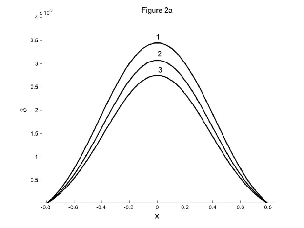
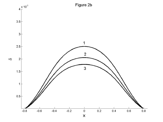
Figure 2: a) The dependence of the relative density perturbation $\delta$ along the field line at $L=6$ and $B_{10}=10^{-5}$ G. The curve $1$ corresponds to $H_{0}=0$, curve $2$ - $H_{0}=0.5$, curve $3$ - $H_{0}=1.0$. b) The same as in Fig. 2a at $L=10$.

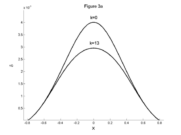
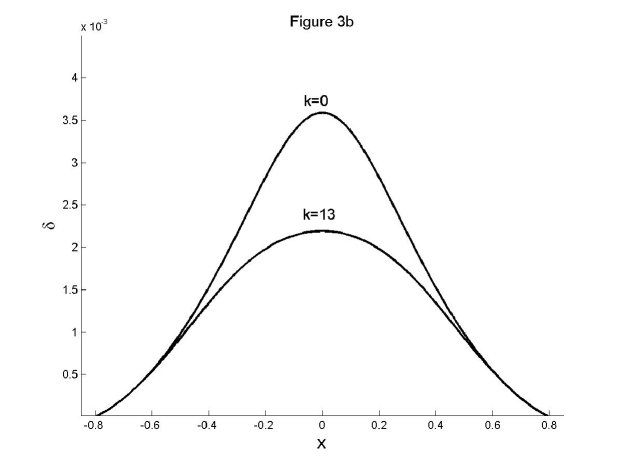
Figure 3: a) The dependence of $\delta$-distribution on $x$ in the dipole ($k=0$) and two-dipole ($k=13$) geomagnetic field at $L=8$ for $B_{10}=10^{-5}$ G and $H_{0}=0$. b) The same as in Fig. 3a for $H_{0}=1.0$.

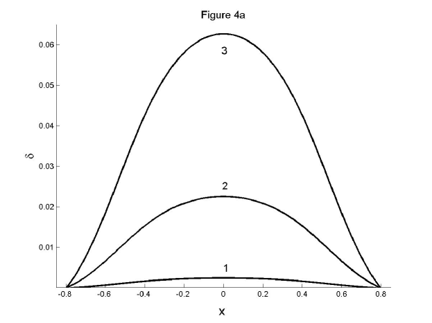
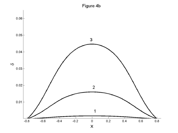
Figure 4: a) The dependence of the relative density perturbation $\delta$ on $x$ for different values of the wave amplitude $B_{10}=(1,3,5)\times 10^{-5}$ G at $L=10$ and $H_{0}=0$. The curve $1$ corresponds to $B_{10}=10^{-5}$ G, curve $2$ - $B_{10}=3\times 10^{-5}$ G, curve $3$ - $B_{10}=5\times 10^{-5}$ G. b) The same as in Fig. 4a for $H_{0}=1.0$.