High–Order Unstructured Lagrangian One–Step WENO Finite Volume Schemes for Non–conservative Hyperbolic Systems: Applications to Compressible Multi–Phase Flows

Abstract

In this article we present the first better than second order accurate unstructured Lagrangian–type one–step WENO finite volume scheme for the solution of hyperbolic partial differential equations with non–conservative products. The method achieves high order of accuracy in space together with essentially non–oscillatory behaviour using a nonlinear WENO reconstruction operator on unstructured triangular meshes. High order accuracy in time is obtained via a local Lagrangian space–time Galerkin predictor method that evolves the spatial reconstruction polynomials in time within each element. The final one–step finite volume scheme is derived by integration over a moving space–time control volume, where the non–conservative products are treated by a path–conservative approach that defines the jump terms on the element boundaries. The entire method is formulated as an Arbitrary–Lagrangian–Eulerian (ALE) method, where the mesh velocity can be chosen independently of the fluid velocity.

The new scheme is applied to the full seven–equation Baer–Nunziato model of compressible multi–phase flows in two space dimensions. The use of a Lagrangian approach allows an excellent resolution of the solid contact and the resolution of jumps in the volume fraction. The high order of accuracy of the scheme in space and time is confirmed via a numerical convergence study. Finally, the proposed method is also applied to a reduced version of the compressible Baer–Nunziato model for the simulation of free surface water waves in moving domains. In particular, the phenomenon of sloshing is studied in a moving water tank and comparisons with experimental data are provided.

1 Introduction

Multi–phase flow problems, such as liquid-vapour and solid-gas flows are encountered in numerous natural processes, such as avalanches, meteorological flows with cloud formation, volcano explosions, sediment transport in rivers and on the coast, granular flows in landslides, etc., as well as in many industrial applications, e.g., in aerospace engineering, automotive industry, petroleum and chemical process engineering, nuclear reactor safety, paper and food manufacturing and renewable energy production. Most of the industrial applications are concerned with compressible multi–phase flows as they appear for example in combustion processes of liquid and solid fuels in car, aircraft and rocket engines, but also in solid bio–mass combustion processes. Already the mathematical description of such flows is quite complex and up to now there is no universally agreed model for such flows. One wide–spread model is the Baer–Nunziato model for compressible two-phase flow, which has been introduced by Baer and Nunziato in [7] for detonation waves in solid–gas combustion processes and which has been further extended by Saurel and Abgrall to liquid–gas flows in [119]. It is therefore also often called in literature the Saurel–Abgrall model. The main difference between the original Baer–Nunziato model and the Saurel–Abgrall model is the definition of the pressure and velocity at the interface. In the present paper, we will use the original choice of Baer–Nunziato, which has also been used in several papers about the exact solution of the Riemann–Problem of the Baer–Nunziato model, see [5, 39, 120]. A reduced five–equation model has been proposed in [102] and approximate Riemann solvers of Baer–Nunziato–type models of compressible multi–phase flows can be found for example in [51, 55, 129, 127].

The full seven–equation Baer–Nunziato model with inter-phase drag and pressure relaxation is given by the following non–conservative system of partial differential equations:

$$\left.\begin{array}[]{l}\par\par\frac{\partial}{\partial t}\left(\phi_{1}\rho_{1}\right)+\nabla\cdot\left(\phi_{1}\rho_{1}\textbf{u}_{\textbf{1}}\right)=0,\par\\ \frac{\partial}{\partial t}\left(\phi_{1}\rho_{1}\textbf{u}_{\textbf{1}}\right)+\nabla\cdot\left(\phi_{1}\rho_{1}\textbf{u}_{\textbf{1}}\textbf{u}_{\textbf{1}}\right)+\nabla\phi_{1}p_{1}=p_{I}\nabla\phi_{1}-\lambda\left(\textbf{u}_{\textbf{1}}-\textbf{u}_{\textbf{2}}\right),\par\\ \frac{\partial}{\partial t}\left(\phi_{1}\rho_{1}E_{1}\right)+\nabla\cdot\left(\left(\phi_{1}\rho_{1}E_{1}+\phi_{1}p_{1}\right)\textbf{u}_{\textbf{1}}\right)=-p_{I}\partial_{t}\phi_{1}-\lambda\,\mathbf{u_{I}}\cdot\left(\mathbf{u_{1}}-\mathbf{u_{2}}\right),\par\\ \frac{\partial}{\partial t}\left(\phi_{2}\rho_{2}\right)+\nabla\cdot\left(\phi_{2}\rho_{2}\textbf{u}_{\textbf{2}}\right)=0,\par\\ \frac{\partial}{\partial t}\left(\phi_{2}\rho_{2}\textbf{u}_{\textbf{2}}\right)+\nabla\cdot\left(\phi_{2}\rho_{2}\textbf{u}_{\textbf{2}}\textbf{u}_{\textbf{2}}\right)+\nabla\phi_{2}p_{2}=p_{I}\nabla\phi_{2}-\lambda\,\left(\textbf{u}_{\textbf{2}}-\textbf{u}_{\textbf{1}}\right),\par\\ \frac{\partial}{\partial t}\left(\phi_{2}\rho_{2}E_{2}\right)+\nabla\cdot\left(\left(\phi_{2}\rho_{2}E_{2}+\phi_{2}p_{2}\right)\textbf{u}_{\textbf{2}}\right)=p_{I}\partial_{t}\phi_{1}-\lambda\,\mathbf{u_{I}}\cdot\left(\mathbf{u_{2}}-\mathbf{u_{1}}\right),\par\\ \frac{\partial}{\partial t}\phi_{1}+\textbf{u}_{\textbf{I}}\nabla\phi_{1}=\nu(p_{1}-p_{2}).\end{array}\right\}$$ (1)

In the entire article, the system is closed by the so-called stiffened gas equation of state (EOS) for each phase:

$$e_{k}=\frac{p_{k}+\gamma_{k}\pi_{k}}{\rho_{k}(\gamma_{k}-1)}.$$ (2)

Here, $\phi_{k}$ denotes the volume fraction of phase $k$, $\rho_{k}$ is the density, $\mathbf{u_{k}}$ is the velocity vector, $E_{k}=e_{k}+\frac{1}{2}\mathbf{u_{k}}^{2}$ and $e_{k}$ are the phase specific total and internal energies, respectively, $\lambda$ is a parameter characterizing the friction between both phases and $\nu$ characterizes pressure relaxation. For consistency the sum of the volume fractions must always be unity, i.e. $\phi_{1}+\phi_{2}=1$. In the literature, one of the phases is often also called the solid phase and the other one the gas phase. Defining arbitrarily the first phase as the solid phase in the rest of the paper we will therefore use the subscripts $1$ and $s$ as well as $2$ and $g$ as synonyms. For the interface velocity and pressure $\mathbf{u_{I}}$ and $p_{I}$ we choose $\mathbf{u_{I}}=\mathbf{u_{1}}$ and $p_{I}=p_{2}$ respectively, according to [7], although other choices are possible, see e.g. the paper by Saurel and Abgrall [119]. We can cast system (1) in the general non-conservative form (3) below

$$\frac{\partial\mathbf{Q}}{\partial t}+\nabla\cdot\mathbf{F}(\mathbf{Q})+\mathbf{B}(\mathbf{Q})\cdot\nabla\mathbf{Q}=\mathbf{S}(\mathbf{Q}),\qquad\mathbf{x}\in\Omega\subset\mathds{R}^{2},t\in\mathds{R}_{0}^{+}$$ (3)

where $\mathbf{Q}=\left(\phi_{1}\rho_{1},\,\phi_{1}\rho_{1}\mathbf{u}_{1},\,\phi_{1}\rho_{1}E_{1},\,\phi_{2}\rho_{2},\,\phi_{2}\rho_{2}\mathbf{u}_{2},\,\phi_{2}\rho_{2}E_{2},\,\phi_{1}\right)\in\Omega_{Q}\subset\mathds{R}^{\nu}$ is the state vector, $\mathbf{F}=(\mathbf{f},\mathbf{g})$ is the flux tensor, i.e. the purely conservative part of the PDE system, $\mathbf{B}=(\mathbf{B}_{1},\mathbf{B}_{2})$ contains the purely non-conservative part of the system in block–matrix notation and $\mathbf{S}(\mathbf{Q})$ is the vector of algebraic source terms, which, in our case, contains the inter–phase drag and the pressure relaxation terms.
We furthermore introduce the abbreviation $\mathbf{P}=\mathbf{P}(\mathbf{Q},\nabla\mathbf{Q})=\mathbf{B}(\mathbf{Q})\cdot\nabla\mathbf{Q}$. System (3) can also be written equivalently in the following quasi–linear form

$$\frac{\partial\mathbf{Q}}{\partial t}+\mathbf{A}(\mathbf{Q})\cdot\nabla\mathbf{Q}=\mathbf{S}(\mathbf{Q}),$$ (4)

with $\mathbf{A}(\mathbf{Q})=(\mathbf{A}_{1},\mathbf{A}_{2})=\partial\mathbf{F}(\mathbf{Q})/\partial\mathbf{Q}+\mathbf{B}(\mathbf{Q})$. The fluxes $\mathbf{F}$, the system matrix $\mathbf{A}(\mathbf{Q})$ and the source term vector $\mathbf{S}(\mathbf{Q})$ can be readily computed from (1). Hyperbolicity of the Baer–Nunziato model and exact Riemann solvers have been studied in [5, 39, 120]. A very important requirement for numerical methods used to solve the Baer–Nunziato model is the sharp resolution of material interfaces, i.e. jumps in the volume fractions $\phi_{k}$. Improved resolution of the material interfaces can be achieved using high order finite volume methods together with little diffusive Riemann solvers, such as the Osher scheme and the HLLC method, both of which have already been successfully applied to the Baer–Nunziato model in [55] and [129], respectively. However, if the interface velocity is small compared to the sound speed of at least one of the two phases, significant numerical smearing of the material contact will occur even with high order schemes and little diffusive Riemann solvers due to the small CFL number associated with the material wave. It may therefore be necessary to further improve the resolution of material interfaces by using a Lagrangian method instead of an Eulerian one, since in the Lagrangian case the mesh moves with the flow field and therefore allows a sharp tracking of material interfaces independent of the CFL number associated with the material contact wave.

The significantly improved resolution of material interfaces led to intensive research on Lagrangian schemes in the past decades. The construction of Lagrangian schemes can start either directly from the conservative quantities such as mass, momentum and total energy [95, 124], or from the nonconservative form of the governing equations, as proposed in [14, 20, 136]. Furthermore existing Lagrangian schemes can be divided into staggered mesh and cell–centered approaches, or combinations of them [90]. Cell centered Godunov–type finite volume schemes together with the first Roe linearization for Lagrangian gas dynamics have been proposed by Munz in [101]. Munz found that in the Lagrangian framework, the Roe–averaged velocity for the equations of gas dynamics is simply given by the arithmetic mean, while in the Eulerian frame the Roe average is a more complicated function of the left and right densities and velocities. A cell-centered Godunov scheme has been proposed by Carré et al. [21] for Lagrangian gas dynamics on general multi-dimensional unstructured meshes and in [40] Després and Mazeran introduce a new formulation of the multidimensional Euler equations in Lagrangian coordinates as a system of conservation laws associated with constraints. Furthermore they propose a way to evolve in a coupled manner both the physical and the geometrical part of the system [41], writing the two–dimensional equations of gas dynamics in Lagrangian coordinates together with the evolution of the geometry as a weakly hyperbolic system of conservation laws. This allows the authors to design a finite volume scheme for the discretization of Lagrangian gas dynamics on moving meshes, based on the symmetrization of the formulation of the physical part. In a recent work Després et al. [36] propose a new method designed for cell-centered Lagrangian schemes, which is translation invariant and suitable for curved meshes. General polygonal grids have been considered by Maire et al. [94, 92, 91], who develop a general formalism to derive first and second order cell-centered Lagrangian schemes in multiple space dimensions. By the use of a node-centered solver [94], the authors obtain the time derivatives of the fluxes and hence a second order method in space and time. Lagrangian schemes for multi–material flows have been successfully introduced in [18, 15, 19] and Lagrangian schemes with additional symmetry preserving properties in cylindrical geometries have been proposed for example in [33, 34, 93, 89]. A multi–scale cell centered Godunov–type finite volume scheme for Lagrangian hydrodynamics has been introduced in [96]. All the Lagrangian schemes listed before are at most second order accurate in space and time.

Cheng and Shu were the first to introduce a third order accurate essentially non-oscillatory (ENO) reconstruction operator into Godunov–type Lagrangian finite volume schemes [32, 87]. Their cell centered Lagrangian finite volume methods achieve also high order in time, either by using the method of lines (MOL) approach based on a third order TVD Runge-Kutta time discretization, or by using a high order one–step Lax-Wendroff-type time stepping. Higher order unstructured Lagrangian finite element methods have been recently investigated in [108, 121]. In a very recent paper Dumbser et al. [56] propose a new class of high order accurate Lagrangian–type one- step WENO finite volume schemes for the solution of stiff hyperbolic balance laws. In [16] this class of high order one–step Lagrangian WENO finite volume schemes has been extended to unstructured triangular meshes for the conservative case and for single–phase flows. The present paper is concerned with its extension to non–conservative systems and applications to compressible multi–phase flows. To our knowledge, the work presented in this article is the first better than second order accurate unstructured Lagrangian–type finite volume scheme for non–conservative hyperbolic systems with applications to compressible multi–phase flows.

To round–off this introduction, we briefly refer also to other Lagrangian–type schemes and alternative Eulerian schemes with improved resolution of material interfaces. The following list of references does not pretend to be complete. Among alternative Lagrangian schemes one should also mention for example meshless particle schemes, such as the smooth particle hydrodynamics (SPH) method [98, 64, 65, 66], which has been successfully used to simulate flows in complex domains with large deformations. Since the SPH approach is a fully Lagrangian method the mesh moves with the local fluid velocity, whereas in Arbitrary Lagrangian Eulerian (ALE) schemes, see e.g. [74, 113, 124, 42, 63, 62, 27], the mesh moves with an arbitrary mesh velocity that does not necessarily coincide with the real fluid velocity. This adds an extra degree of flexibility and generality to the scheme. The classical SPH method is a truly meshless scheme, but exhibits also a series of problems, such as the need for artificial stabilization terms and the lack of zeroth order consistency. These problems have been overcome by the so–called Particle Finite Element Method (PFEM), which is a Lagrangian (or Arbitrary–Lagrangian–Eulerian) finite element scheme on moving point clouds, [78, 114, 107, 84, 79, 106], and has been successfully applied to incompressible multi–material flows and fluid–solid interaction problems. Furthermore, the reader will also find so–called Semi-Lagrangian schemes in literature, which are mainly used for solving transport equations [118, 71]. Here, the numerical solution at the new time is computed from the known solution at the current time by following backward in time the Lagrangian trajectories of the fluid to the foot–point of the trajectory. Semi–Lagrangian schemes are therefore nothing else than a numerical scheme based on the method of characteristics. Since in general the end-point does not coincide with a grid point, an interpolation formula is required in order to evaluate the unknown solution, see e.g. [25, 26, 86, 77, 115, 38, 17]. Note that in Semi-Lagrangian algorithms the mesh is fixed, like in a classical Eulerian methods. An alternative to Lagrangian methods for the accurate resolution of material interfaces has been developed in the Eulerian framework on fixed meshes under the form of ghost–fluid and level–set methods [60, 61, 67, 109, 100], as well as the volume of fluid method [75, 117, 88].

The rest of the paper is organized as follows: in Section 2 the high–order path–conservative Arbitrary–Lagrangian–Eulerian (ALE) one–step WENO finite volume scheme is described on unstructured triangular meshes and a numerical convergence study on a smooth unsteady test problem is carried out, to assess the designed order of accuracy of the scheme in space and time. In Section 3 some classical academic benchmark problems with exact or quasi–exact reference solution are solved to verify the robustness of the method in the presence of shock waves and significant mesh distorsion. Finally, in Section 4 our new high order path–conservative ALE method is applied to a free–surface flow problem concerning sloshing in a moving tank. For this purpose, a reduced version of the Baer–Nunziato model is solved, which has been introduced for the simulation of free surface flows on fixed grids in [46, 44]. The paper is rounded–off by some concluding remarks and an outlook to future research in Section 5.

2 Numerical Method

The time–dependent computational domain is denoted by $\Omega(t)\subset\mathds{R}^{2}$ and is discretized at a given time $t^{n}$ by a set of conforming triangles $T^{n}_{i}$, the union of which is the current triangulation $\mathcal{T}^{n}_{\Omega}$ of the domain $\Omega(t^{n})=\Omega^{n}$ and can be expressed as

$$\mathcal{T}^{n}_{\Omega}=\bigcup\limits_{i=1}^{N_{E}}{T^{n}_{i}}.$$ (5)

Here, $N_{E}$ is the number of elements used to discretize the domain.

On triangular meshes it is convenient to introduce also a local spatial reference coordinate system $\xi-\eta$, which maps the physical element $T_{i}^{n}$ in the current configuration to the reference element denoted by $T_{e}$. The spatial mapping reads

$$\mathbf{x}=\mathbf{x}(\boldsymbol{\xi},t^{n})=\mathbf{X}^{n}_{1,i}+\left(\mathbf{X}^{n}_{2,i}-\mathbf{X}^{n}_{1,i}\right)\xi+\left(\mathbf{X}^{n}_{3,i}-\mathbf{X}^{n}_{1,i}\right)\eta$$ (6)

where $\boldsymbol{\xi}=(\xi,\eta)$ and $\mathbf{x}=(x,y)$ are the vectors of the spatial coordinates in the reference system and the physical system, respectively, and $\mathbf{X}^{n}_{k,i}=(X^{n}_{k,i},Y^{n}_{k,i})$ is the vector of physical coordinates of the $k$-th vertex of triangle $T^{n}_{i}$ at time $t^{n}$. The unit triangle $T_{e}$ is defined by the nodes $\boldsymbol{\xi}_{e,1}=(\xi_{e,1},\eta_{e,1})=(0,0)$, $\boldsymbol{\xi}_{e,2}=(\xi_{e,2},\eta_{e,2})=(1,0)$ and $\boldsymbol{\xi}_{e,3}=(\xi_{e,2},\eta_{e,2})=(0,1)$.

The cell averages, which represent the data that are stored and evolved in time within a finite volume scheme, are defined at time $t^{n}$ as usual by

$$\mathbf{Q}_{i}^{n}=\frac{1}{|T_{i}^{n}|}\int_{T^{n}_{i}}\mathbf{Q}(\mathbf{x},t^{n})d\mathbf{x}.$$ (7)

Here, $|T_{i}^{n}|$ denotes the area of triangle $T_{i}^{n}$. Higher order in space can be achieved by reconstructing piecewise higher order polynomials $\mathbf{w}_{h}(\mathbf{x},t^{n})$ from the cell averages defined above in Eqn. (7). For this purpose, we employ a higher order WENO reconstruction procedure following [82, 52, 53]. Other WENO schemes on structured and unstructured meshes can be found, e.g., in [9, 80] and [68, 128, 133, 76, 138, 3], respectively. Instead of a WENO method, alternative high order nonlinear reconstruction operators can be used as well, see e.g. [125, 1, 35]. For the convenience of the reader, the component–wise WENO reconstruction procedure is briefly summarized in the next section, for details we refer to [52]. A possible polynomial WENO reconstruction in characteristic variables can be found in [53].

2.1 WENO Reconstruction

The reconstructed solution $\mathbf{w}_{h}(\mathbf{x},t^{n})$ is represented by piecewise polynomials of degree $M$ and is obtained from the given cell averages in an appropriate neighborhood of element $T_{i}^{n}$, called the reconstruction stencil $\mathcal{S}_{i}^{s}$. The number of elements inside each reconstruction stencil is denoted by $n_{e}$. In 2D we use in total 7 reconstruction stencils for each element, one central stencil, three forward stencils and three backward stencils, as proposed in [82, 52], hence $1\leq s\leq 7$. According to [12] the total number of stencil elements $n_{e}$ must be larger than the number of degrees of freedom $\mathcal{M}=(M+1)(M+2)/2$ of a polynomial of degree $M$. Typically we take $n_{e}=2\mathcal{M}$ in two space dimensions.

The reconstruction polynomial for each candidate stencil $s$ for triangle $T_{i}^{n}$ is written in terms of spatial basis functions $\psi_{l}(\boldsymbol{\xi})$ as

$$\mathbf{w}^{s}_{h}(\mathbf{x},t^{n})=\sum\limits_{l=1}^{\mathcal{M}}\psi_{l}(\boldsymbol{\xi})\hat{\mathbf{w}}^{n,s}_{l,i}:=\psi_{l}(\boldsymbol{\xi})\hat{\mathbf{w}}^{n,s}_{l,i},$$ (8)

where the mapping $\mathbf{x}=\mathbf{x}(\boldsymbol{\xi},t^{n})$ is given by Eqn. (6). In the rest of the paper we will use classical tensor index notation based on the Einstein summation convention, which implies summation over two equal indices. The number of the unknown degrees of freedom to be reconstructed for each element is $\mathcal{M}$. The basis functions $\psi_{l}(\boldsymbol{\xi})$ are the orthogonal basis functions described in [43, 81, 37].

The reconstruction on each stencil $\mathcal{S}_{i}^{s}$ is based on integral conservation, i.e.

$$\frac{1}{|T^{n}_{j}|}\int\limits_{T^{n}_{j}}\psi_{l}(\boldsymbol{\xi})\hat{\mathbf{w}}^{n,s}_{l,i}d\mathbf{x}=\mathbf{Q}^{n}_{j},\qquad\forall T^{n}_{j}\in\mathcal{S}_{i}^{s}.$$ (9)

Since $n_{e}>\mathcal{M}$ the above system (9) is an over–determined linear algebraic system that is solved for $\hat{\mathbf{w}}^{n,s}_{l,i}$ using a constrained least–squares technique, see [52]. The linear constraint is that Eqn. (9) holds exactly at least for element $T_{i}^{n}$. The multi–dimensional integrals appearing in the expression above are evaluated using Gaussian quadrature formulae of suitable order, see [126] for details. Since the triangles are moving in a Lagrangian scheme, the small linear systems (9) are solved for each element at the beginning of each time step. However, the choice of the stencils $\mathcal{S}_{i}^{s}$ remains fixed for all times.

To obtain a higher order essentially non–oscillatory polynomial the scheme must be nonlinear, in order to circumvent the Godunov theorem that states that linear monotone schemes are at most of order one. The final nonlinear WENO reconstruction polynomial is therefore computed in the following way. First, the smoothness of each reconstruction polynomial obtained on stencil $\mathcal{S}_{i}^{s}$ is measured by a so–called oscillation indicator $\boldsymbol{\sigma}_{s}$ [80]. According to [52] the smoothness indicator can be easily computed on the reference element using the (universal) oscillation indicator matrix $\boldsymbol{\Sigma}_{lm}$ as follows:

$$\boldsymbol{\sigma}_{s}=\boldsymbol{\Sigma}_{lm}\hat{\mathbf{w}}^{n,s}_{l,i}\hat{\mathbf{w}}^{n,s}_{m,i},\qquad\boldsymbol{\Sigma}_{lm}=\sum\limits_{\alpha+\beta\leq M}\,\,\int\limits_{T_{e}}\frac{\partial^{\alpha+\beta}\psi_{l}(\boldsymbol{\xi})}{\partial\xi^{\alpha}\partial\eta^{\beta}}\cdot\frac{\partial^{\alpha+\beta}\psi_{m}(\boldsymbol{\xi})}{\partial\xi^{\alpha}\partial\eta^{\beta}}d\xi d\eta.$$ (10)

The nonlinear weights $\boldsymbol{\omega}_{s}$ are defined by

$$\tilde{\boldsymbol{\omega}}_{s}=\frac{\lambda_{s}}{\left(\sigma_{s}+\epsilon\right)^{r}},\qquad\boldsymbol{\omega}_{s}=\frac{\tilde{\boldsymbol{\omega}}_{s}}{\sum_{q}\tilde{\boldsymbol{\omega}}_{q}},$$ (11)

where we use $\epsilon=10^{-14}$, $r=8$, $\lambda_{s}=1$ for the one–sided stencils and $\lambda_{s}=10^{5}$ for the central stencil, according to [52]. The final nonlinear WENO reconstruction polynomial and its coefficients are then given by

$$\mathbf{w}_{h}(\mathbf{x},t^{n})=\sum\limits_{l=1}^{\mathcal{M}}\psi_{l}(\boldsymbol{\xi})\hat{\mathbf{w}}^{n}_{l,i},\qquad\textnormal{ with }\qquad\hat{\mathbf{w}}^{n}_{l,i}=\sum_{s}\boldsymbol{\omega}_{s}\hat{\mathbf{w}}^{n,s}_{l,i}.$$ (12)

In order to reduce the computational cost associated with the nonlinear WENO reconstruction procedure outlined above, a high order one–step time discretization is used so that reconstruction has to be performed only once for each time step.

2.2 Local Space–Time Predictor on Moving Curved Meshes

Higher order of accuracy in time is achieved by an element–local predictor stage that evolves the reconstructed polynomials $\mathbf{w}_{h}(\mathbf{x},t^{n})$ locally in time within each element $T_{i}(t)$ during the time interval $[t^{n};t^{n+1}]$, see [50, 47, 51, 72, 69]. Such an element–local time–evolution procedure has also been used within the MUSCL scheme of van Leer [134] and the original ENO scheme of Harten et al. [70], who called this element–local predictor with initial data $\mathbf{w}_{h}(\mathbf{x},t^{n})$ the solution of a Cauchy problem in the small, since no information from neighbor elements is used. The coupling with the neighbor elements occurs only later in the final one–step finite volume scheme.

The local data evolution step leads for each element to piecewise space–time polynomials of degree $M$, denoted by $\mathbf{q}_{h}(\mathbf{x},t)$ in the following. While the original ENO scheme of Harten et al. uses a higher order Taylor series in time together with the strong differential form of the PDE to substitute time–derivatives with space derivatives (the so–called Cauchy–Kovalewski or Lax–Wendroff procedure [85]), here a weak formulation of the PDE in space–time is used. The resulting method does not require the computation of higher order derivatives, but just pointwise evaluations of the fluxes, source terms and non–conservative products appearing in the PDE. Such a local space–time Galerkin predictor scheme was introduced for the Eulerian framework in [50, 47, 51, 72] and is extended here to the Lagrangian framework on moving curved space–time elements for PDE with nonconservative products.

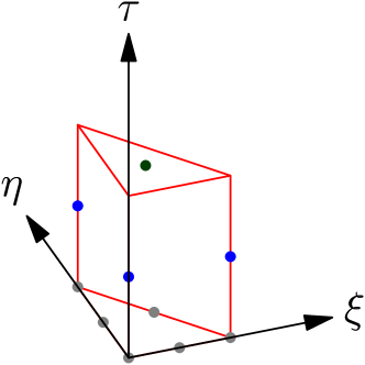
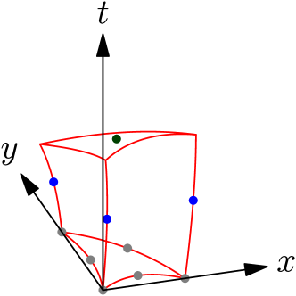
Figure 1: Iso–parametric mapping of the space–time reference element (left) to the physical space–time element (right) used within the local space–time Galerkin predictor.

Let $\mathbf{\tilde{x}}=(x,y,t)$ denote the physical space–time coordinate vector and $\boldsymbol{\tilde{\xi}}=(\xi,\eta,\tau)$ the reference space–time coordinate vector, while $\mathbf{x}=(x,y)$ and $\boldsymbol{\xi}=(\xi,\eta)$ are the purely spatial coordinate vectors already introduced previously. Let furthermore $\theta_{l}=\theta_{l}(\boldsymbol{\tilde{\xi}})=\theta_{l}(\xi,\eta,\tau)$ be a space–time basis function defined by the Lagrange interpolation polynomials passing through the space–time nodes $\boldsymbol{\tilde{\xi}}_{m}=(\xi_{m},\eta_{m},\tau_{m})$ specified according to [47] and also depicted for the case $M=2$ in Figure 1. The Lagrange interpolation polynomials define a nodal basis which satisfies the interpolation property

$$\theta_{l}(\boldsymbol{\tilde{\xi}}_{m})=\delta_{lm},$$ (13)

with the usual Kronecker symbol $\delta_{lm}$. The element–local space -time predictor solution $\mathbf{q}_{h}$, the fluxes $\mathbf{F}_{h}=(\mathbf{f}_{h},\mathbf{g}_{h})$, the source term $\mathbf{S}_{h}$ and the non–conservative product $\mathbf{P}_{h}=\mathbf{B}(\mathbf{q}_{h})\cdot\nabla\mathbf{q}_{h}$ are approximated within the space–time element $T_{i}(t)\times[t^{n};t^{n+1}]$ as

$$\mathbf{q}_{h}=\mathbf{q}_{h}(\boldsymbol{\tilde{\xi}})=\theta_{l}(\boldsymbol{\tilde{\xi}})\,\widehat{\mathbf{q}}_{l,i},\qquad\qquad\mathbf{F}_{h}=\mathbf{F}_{h}(\boldsymbol{\tilde{\xi}})=\theta_{l}(\boldsymbol{\tilde{\xi}})\,\widehat{\mathbf{F}}_{l,i},$$

$$\mathbf{S}_{h}=\mathbf{S}_{h}(\boldsymbol{\tilde{\xi}})=\theta_{l}(\boldsymbol{\tilde{\xi}})\,\widehat{\mathbf{S}}_{l,i},\qquad\qquad\mathbf{P}_{h}=\mathbf{P}_{h}(\boldsymbol{\tilde{\xi}})=\theta_{l}(\boldsymbol{\tilde{\xi}})\,\widehat{\mathbf{P}}_{l,i}.$$ (14)

Since a nodal basis is used, the degrees of freedom for $\mathbf{F}_{h}$, $\mathbf{S}_{h}$ and $\mathbf{P}_{h}$ can be simply computed pointwise from $\mathbf{q}_{h}$ as

$$\widehat{\mathbf{F}}_{l,i}=\mathbf{F}(\widehat{\mathbf{q}}_{l,i}),\quad\widehat{\mathbf{S}}_{l,i}=\mathbf{S}(\widehat{\mathbf{q}}_{l,i}),\quad\widehat{\mathbf{P}}_{l,i}=\mathbf{P}(\widehat{\mathbf{q}}_{l,i},\nabla\widehat{\mathbf{q}}_{l,i}),\quad\widehat{\nabla\mathbf{q}}_{l,i}=\nabla\theta_{m}(\boldsymbol{\tilde{\xi}}_{l})\widehat{\mathbf{q}}_{m,i}.$$ (15)

The degrees of freedom $\widehat{\nabla\mathbf{q}}_{l,i}$ represent the gradient of $\mathbf{q}_{h}$ in node $\boldsymbol{\tilde{\xi}}_{l}$.

In the present paper an isoparametric mapping is used between the physical space–time coordinate vector $\mathbf{\tilde{x}}$ and the reference space–time coordinate vector $\boldsymbol{\tilde{\xi}}$, i.e. the mapping is also represented by the nodal basis functions $\theta_{l}$. Hence,

$$\mathbf{x}(\boldsymbol{\tilde{\xi}})=\theta_{l}(\boldsymbol{\tilde{\xi}})\,\widehat{\mathbf{x}}_{l,i},\qquad t(\boldsymbol{\tilde{\xi}})=\theta_{l}(\boldsymbol{\tilde{\xi}})\,\widehat{t}_{l},$$ (16)

where the degrees of freedom $\widehat{\mathbf{x}}_{l,i}=(\widehat{x}_{l,i},\widehat{y}_{l,i})$ denote the in general unknown vector of physical coordinates in space of the moving space–time control volume and the $\widehat{t}_{l}$ denote the known degrees of freedom of the physical time at each space–time node $\tilde{\mathbf{x}}_{l,i}=(\widehat{x}_{l,i},\widehat{y}_{l,i},\widehat{t}_{l})$. The general representation of the mapping in time given above in Eqn. (16) simplifies to

$$t=t_{n}+\tau\,\Delta t,\qquad\tau=\frac{t-t^{n}}{\Delta t},\qquad\Rightarrow\qquad\widehat{t}_{l}=t_{n}+\tau_{l}\,\Delta t,$$ (17)

where $t^{n}$ is the current time and $\Delta t$ is the time step. Hence, $t_{\xi}=t_{\eta}=0$ and $t_{\tau}=\Delta t$. The isoparametric mapping (16) allow us to transform the physical space–time element to the unit reference space–time element $T_{e}\times[0,1]$. A sketch of this mapping is depicted in Figure 1 and the Jacobian matrix of the transformation reads

$$J_{st}=\frac{\partial\mathbf{\tilde{x}}}{\partial\boldsymbol{\tilde{\xi}}}=\left(\begin{array}[]{ccc}x_{\xi}&x_{\eta}&x_{\tau}\\ y_{\xi}&y_{\eta}&y_{\tau}\\ 0&0&\Delta t\\ \end{array}\right).$$ (18)

Its inverse is given by

$$J_{st}^{-1}=\frac{\partial\boldsymbol{\tilde{\xi}}}{\partial\mathbf{\tilde{x}}}=\left(\begin{array}[]{ccc}\xi_{x}&\xi_{y}&\xi_{t}\\ \eta_{x}&\eta_{y}&\eta_{t}\\ 0&0&\frac{1}{\Delta t}\\ \end{array}\right).$$ (19)

The local reference system and the inverse of the associated Jacobian matrix (19) are used to rewrite the governing PDE (3) as

$$\frac{\partial\mathbf{Q}}{\partial\tau}+\Delta t\left[\frac{\partial\mathbf{Q}}{\partial\boldsymbol{\xi}}\cdot\frac{\partial\boldsymbol{\xi}}{\partial t}+\left(\frac{\partial\boldsymbol{\xi}}{\partial\mathbf{x}}\right)^{T}\nabla_{\boldsymbol{\xi}}\cdot\mathbf{F}+\mathbf{B}(\mathbf{Q})\cdot\left(\frac{\partial\boldsymbol{\xi}}{\partial\mathbf{x}}\right)^{T}\nabla_{\boldsymbol{\xi}}\mathbf{Q}\right]=\Delta t\mathbf{S}(\mathbf{Q}),$$ (20)

using $\tau_{x}=\tau_{y}=0$ and $\tau_{t}=\frac{1}{\Delta t}$ according to (17) and with the notation

$$\nabla_{\boldsymbol{\xi}}=\left(\begin{array}[]{c}\frac{\partial}{\partial\xi}\\ \frac{\partial}{\partial\eta}\end{array}\right),\qquad\nabla=\left(\begin{array}[]{c}\frac{\partial}{\partial x}\\ \frac{\partial}{\partial y}\end{array}\right)=\left(\begin{array}[]{cc}\xi_{x}&\eta_{x}\\ \xi_{y}&\eta_{y}\end{array}\right)\left(\begin{array}[]{c}\frac{\partial}{\partial\xi}\\ \frac{\partial}{\partial\eta}\end{array}\right)=\left(\frac{\partial\boldsymbol{\xi}}{\partial\mathbf{x}}\right)^{T}\nabla_{\boldsymbol{\xi}}.$$ (21)

The term $\frac{\partial\mathbf{Q}}{\partial\boldsymbol{\xi}}\cdot\frac{\partial\boldsymbol{\xi}}{\partial t}$ is due to the Lagrangian mesh motion and is zero in the Eulerian case, i.e. for fixed meshes.

We further introduce the abbreviation

$$\mathbf{H}=\Delta t\mathbf{S}-\Delta t\left[\frac{\partial\mathbf{Q}}{\partial\boldsymbol{\xi}}\cdot\frac{\partial\boldsymbol{\xi}}{\partial t}+\left(\frac{\partial\boldsymbol{\xi}}{\partial\mathbf{x}}\right)^{T}\nabla_{\boldsymbol{\xi}}\cdot\mathbf{F}+\mathbf{B}(\mathbf{Q})\cdot\left(\frac{\partial\boldsymbol{\xi}}{\partial\mathbf{x}}\right)^{T}\nabla_{\boldsymbol{\xi}}\mathbf{Q}\right],$$ (22)

and its numerical approximation by

$$\mathbf{H}_{h}=\theta_{l}(\boldsymbol{\tilde{\xi}})\,\widehat{\mathbf{H}}_{l,i},\qquad$$ (23)

as well as the two operators

$$\left[f,g\right]^{\tau}=\int\limits_{T_{e}}f(\boldsymbol{\xi},\tau)g(\boldsymbol{\xi},\tau)d\xi d\eta,\quad\left\langle f,g\right\rangle=\int\limits_{0}^{1}\int\limits_{T_{e}}f(\boldsymbol{\xi},\tau)g(\boldsymbol{\xi},\tau)d\xi d\eta d\tau$$ (24)

that denote the scalar products of two functions $f$ and $g$ over the spatial reference element $T_{e}$ at time $\tau$ and over the space-time reference element $T_{e}\times\left[0,1\right]$, respectively.

Multiplication of (20) with space–time test functions $\theta_{k}(\boldsymbol{\xi})$, integration over the space–time reference element $T_{e}\times[0,1]$ and inserting (14) and (23) yields

$$\left\langle\theta_{k},\frac{\partial\theta_{l}}{\partial\tau}\right\rangle\widehat{\mathbf{q}}_{l,i}=\left\langle\theta_{k},\theta_{l}\right\rangle\widehat{\mathbf{H}}_{l,i}.\\$$

The term on the left hand side can be integrated by parts in time, which also allows to introduce the initial condition of the local Cauchy problem in a weak form as follows:

$$\left[\theta_{k}(\boldsymbol{\xi},1),\theta_{l}(\boldsymbol{\xi},1)\right]^{1}\widehat{\mathbf{q}}_{l,i}-\left\langle\frac{\partial\theta_{k}}{\partial\tau},\theta_{l}\right\rangle\widehat{\mathbf{q}}_{l,i}=\left[\theta_{k}(\boldsymbol{\xi},0),\psi_{l}(\boldsymbol{\xi})\right]^{0}\hat{\mathbf{w}}^{n}_{l,i}+\left\langle\theta_{k},\theta_{l}\right\rangle\widehat{\mathbf{H}}_{l,i}.$$ (25)

With the definitions

$$K_{1}=\left[\theta_{k}(\boldsymbol{\xi},1),\theta_{l}(\boldsymbol{\xi},1)\right]^{1}-\left\langle\frac{\partial\theta_{k}}{\partial\tau},\theta_{l}\right\rangle,\quad\mathbf{F}_{0}=\left[\theta_{k}(\boldsymbol{\xi},0),\psi_{l}(\boldsymbol{\xi})\right],\quad\mathbf{M}=\left\langle\theta_{k},\theta_{l}\right\rangle,$$ (26)

the above expression, which is a nonlinear algebraic equation system for the unknown coefficients $\widehat{\mathbf{q}}_{l,i}$ can be written in a more compact matrix form as

$$K_{1}\widehat{\mathbf{q}}_{l,i}=\mathbf{F}_{0}\hat{\mathbf{w}}^{n}_{l,i}+\mathbf{M}\widehat{\mathbf{H}}_{l,i},$$ (27)

and is conveniently solved using the following iterative scheme:

$$\widehat{\mathbf{q}}_{l,i}^{r+1}=K_{1}^{-1}\left(\mathbf{F}_{0}\hat{\mathbf{w}}^{n}_{l,i}+\mathbf{M}\widehat{\mathbf{H}}_{l,i}^{r}\right),$$ (28)

where $r$ denotes the iteration number. For an efficient initial guess based on a second order MUSCL–type scheme, see [72].

Since the mesh is moving we also have to consider the evolution of the vertex coordinates of the local space–time element, whose motion is described by the ODE system

$$\frac{d\mathbf{x}}{dt}=\mathbf{V}(\mathbf{Q},\mathbf{x},t),$$ (29)

where $\mathbf{V}=\mathbf{V}(\mathbf{Q},\mathbf{x},t)$ is the local mesh velocity. In the Arbitrary Lagrangian-Eulerian (ALE) framework used in this article, the mesh velocity can be chosen independently of the fluid velocity, hence for $\mathbf{V}=0$ the scheme reduces to a pure Eulerian approach, but if $\mathbf{V}$ coincides with the local fluid velocity $\mathbf{v}=\mathbf{v}(\mathbf{Q})$ one obtains a Lagrangian method. The discrete velocity field inside element $T_{i}(t)$ can be expressed as

$$\mathbf{V}_{h}=\theta_{l}(\boldsymbol{\xi},\tau)\widehat{\mathbf{V}}_{l,i},$$ (30)

with $\widehat{\mathbf{V}}_{l,i}=\mathbf{V}(\mathbf{\hat{\mathbf{q}}}_{l,i},\hat{\mathbf{x}}_{l,i},\hat{t}_{l})$.

As in [56] the ODE (29) can be solved for the unknown coordinate vector $\widehat{\mathbf{x}}_{l}$ by using again the local space–time DG method:

$$K_{1}\widehat{\mathbf{x}}_{l,i}=\left[\theta_{k}(\boldsymbol{\xi},0),\mathbf{x}(\boldsymbol{\xi},t^{n})\right]^{0}+\Delta t\mathbf{M}\,\widehat{\mathbf{V}}_{l,i},$$ (31)

with $\mathbf{x}(\boldsymbol{\xi},t^{n})$ given according to the spatial mapping (6) based on the known vertex coordinates of triangle $T_{i}^{n}$ at time $t^{n}$. This results in the following iteration scheme for the element–local space–time predictor for the nodal coordinates:

$$\widehat{\mathbf{x}}^{r+1}_{l,i}=K_{1}^{-1}\left(\left[\theta_{k}(\boldsymbol{\xi},0),\mathbf{x}(\boldsymbol{\xi},t^{n})\right]^{0}+\Delta tM\widehat{\mathbf{V}}^{r}_{l,i}\right).$$ (32)

Eqn. (32) is iterated together with Eqn. (28). The iteration stops when the residuals of (28) and (32) are less than a prescribed tolerance, which we set to $10^{-12}$ for all examples shown below.

Once we have carried out the above procedure for all the elements of the computational domain, we end up with an element–local predictor for the numerical solution $\mathbf{q}_{h}$, as well as for the mesh velocity $\mathbf{V}_{h}$.

Next, we have to update the mesh globally. Let us denote with $\mathcal{V}_{k}$ the neighborhood of vertex number $k$, i.e. all those elements that have in common the node number $k$. The number of elements in the neighborhood $\mathcal{V}_{k}$ is denoted with $N_{k}$. Since the velocity of each vertex is defined by the local predictor within each element, one has to deal with several, in general different, velocities for the same node, since all elements belonging to $\mathcal{V}_{k}$ will in general give a different velocity contribution, according to their element–local predictor. Since we do not admit the geometry to be discontinuous, we decide to fix a unique node velocity $\overline{\mathbf{V}}_{k}^{n}$ to move the node. The final velocity is chosen to be the average velocity considering all the contributions $\overline{\mathbf{V}}_{k,j}^{n}$ of the vertex neighborhood as

$$\overline{\mathbf{V}}_{k}^{n}=\frac{1}{N_{k}}\sum\limits_{T_{j}^{n}\in\mathcal{V}_{k}}{\overline{\mathbf{V}}_{k,j}^{n}},\qquad\textnormal{ with }\qquad\overline{\mathbf{V}}_{k,j}^{n}=\left(\int\limits_{0}^{1}\theta_{l}(\boldsymbol{\xi}_{e,m(k)},\tau)d\tau\right)\widehat{\mathbf{V}}_{l,j}.$$ (33)

The $\boldsymbol{\xi}_{e,m(k)}$ are the vertex coordinates of the reference triangle $T_{e}$ corresponding to vertex number $k$, hence $m=m(k)$ with $1\leq m\leq 3$ is a mapping from the global node number $k$ to the element–local vertex number. Since each node now has its own unique velocity, the vertex coordinates can be moved according to

$$\mathbf{X}^{n+1}_{k}=\mathbf{X}^{n}_{k}+\Delta t\,\overline{\mathbf{V}}_{k}^{n},$$ (34)

and we can update all the other geometric quantities needed for the computation, e.g. normal vectors, volumes, side lengths, barycenter positions, etc.

2.3 Path–Conservative One–Step Finite–Volume Scheme

The governing PDE system (3) can be rewritten more compactly using the following space–time divergence form

$$\tilde{\nabla}\cdot\tilde{\mathbf{F}}+\tilde{\mathbf{B}}(\mathbf{Q})\cdot\tilde{\nabla}\mathbf{Q}=\mathbf{S}(\mathbf{Q}),$$ (35)

with the space–time nabla operator

$$\tilde{\nabla}=\left(\frac{\partial}{\partial x},\,\frac{\partial}{\partial y},\,\frac{\partial}{\partial t}\right)^{T}$$ (36)

and the space–time flux tensor and system matrices

$$\tilde{\mathbf{F}}=\left(\mathbf{f},\,\mathbf{g},\,\mathbf{Q}\right),\qquad\tilde{\mathbf{B}}=(\mathbf{B}_{1},\mathbf{B}_{2},0),\qquad\tilde{\mathbf{A}}=\frac{\partial\tilde{\mathbf{F}}}{\partial\mathbf{Q}}+\tilde{\mathbf{B}}.$$ (37)

With (36) and (37) the quasi–linear form of the PDE (35) reads

$$\tilde{\mathbf{A}}(\mathbf{Q})\cdot\tilde{\nabla}\mathbf{Q}=\mathbf{S}(\mathbf{Q}).$$ (38)

Integration over a space–time control volume $\mathcal{C}^{n}_{i}=T_{i}(t)\times\left[t^{n};t^{n+1}\right]$ yields

$$\int\limits_{\mathcal{C}^{n}_{i}}\tilde{\nabla}\cdot\tilde{\mathbf{F}}\,d\mathbf{x}dt+\int\limits_{\mathcal{C}^{n}_{i}}\tilde{\mathbf{B}}(\mathbf{Q})\cdot\tilde{\nabla}\mathbf{Q}\,d\mathbf{x}dt=\int\limits_{\mathcal{C}^{n}_{i}}\mathbf{S}(\mathbf{Q})\,d\mathbf{x}dt.$$ (39)

Application of the theorem of Gauss allows us to write the first space–time volume integral on the left as a flux integral over the space–time surface $\partial\mathcal{C}^{n}_{i}$. Furthermore, the non–conservative product is integrated by using a path–conservative approach [132, 112, 111, 23, 99, 22, 116, 49, 51, 55], which follows the theory of Dal Maso–Le Floch and Murat [97] and defines the non–conservative term as a Borel measure. For the known limitations and deficiencies of path–conservative schemes see [24, 2]. Thus

$$\int\limits_{\partial\mathcal{C}^{n}_{i}}\left(\tilde{\mathbf{F}}+\tilde{\mathbf{D}}\right)\cdot\ \mathbf{\tilde{n}}\,dS+\!\!\int\limits_{\mathcal{C}^{n}_{i}\backslash\partial\mathcal{C}^{n}_{i}}\!\!\!\tilde{\mathbf{B}}(\mathbf{Q})\cdot\tilde{\nabla}\mathbf{Q}\,d\mathbf{x}dt=\int\limits_{\mathcal{C}^{n}_{i}}\mathbf{S}(\mathbf{Q})\,d\mathbf{x}dt,$$ (40)

where $\mathbf{\tilde{n}}=(\tilde{n}_{x},\tilde{n}_{y},\tilde{n}_{t})$ is the outward pointing space–time unit normal vector on the space–time surface $\partial C^{n}_{i}$, and $\tilde{\mathbf{D}}$ is a term that takes into account potential jumps of $\mathbf{Q}$ on the element boundaries according to the path integral

$$\tilde{\mathbf{D}}\cdot\mathbf{\tilde{n}}=\int\limits_{0}^{1}\tilde{\mathbf{B}}\left(\boldsymbol{\Psi}(\mathbf{Q}^{-},\mathbf{Q}^{+},s)\right)\cdot\mathbf{\tilde{n}}\,\frac{\partial\boldsymbol{\Psi}}{\partial s}\,ds.$$ (41)

Throughout the entire paper and according to [111, 23, 51, 55] we use the following straight–line segment path

$$\boldsymbol{\Psi}=\boldsymbol{\Psi}(\mathbf{Q}^{-},\mathbf{Q}^{+},s)=\mathbf{Q}^{-}+s(\mathbf{Q}^{+}-\mathbf{Q}^{-}),$$ (42)

for which the jump term above (41) simplifies to

$$\tilde{\mathbf{D}}\cdot\mathbf{\tilde{n}}=\left(\int\limits_{0}^{1}\tilde{\mathbf{B}}\left(\boldsymbol{\Psi}(\mathbf{Q}^{-},\mathbf{Q}^{+},s)\right)\cdot\mathbf{\tilde{n}}\,ds\right)\left(\mathbf{Q}^{+}-\mathbf{Q}^{-}\right).$$ (43)

The space–time surface $\partial C^{n}_{i}$ above involves overall five space–time sub–surfaces, as depicted in Figure 2:

$$\partial C^{n}_{i}=\left(\bigcup\limits_{T_{j}(t)\in\mathcal{N}_{i}}\partial C^{n}_{ij}\right)\,\,\cup\,\,T_{i}^{n}\,\,\cup\,\,T_{i}^{n+1},$$ (44)

where $\mathcal{N}_{i}$ denotes the so–called Neumann neighborhood of triangle $T_{i}(t)$, i.e. the set of directly adjacent triangles $T_{j}(t)$ that share a common edge $\partial T_{ij}(t)$ with triangle $T_{i}(t)$. The common space–time edge $\partial C^{n}_{ij}$ during the time interval $[t^{n};t^{n+1}]$ is denoted above by $\partial C^{n}_{ij}=\partial T_{ij}(t)\times[t^{n};t^{n+1}]$.

The upper space–time sub–surface $T_{i}^{n+1}$ and the lower space–time sub–surface $T_{i}^{n}$ are parametrized by $0\leq\xi\leq 1\wedge 0\leq\eta\leq 1-\xi$ and the mapping (6). They are orthogonal to the time coordinate, hence for these faces the space–time unit normal vectors simply read $\mathbf{\tilde{n}}=(0,0,1)$ for $T_{i}^{n+1}$ and $\mathbf{\tilde{n}}=(0,0,-1)$ for $T_{i}^{n}$, respectively. The lateral space–time sub–faces $\partial C^{n}_{ij}$ are defined using a simple bilinear parametrization, since the old vertex coordinates $\mathbf{X}_{ik}^{n}$ are given and the new ones $\mathbf{X}_{ik}^{n+1}$ are known from (34).

$$\partial C_{ij}^{n}=\mathbf{\tilde{x}}\left(\chi,\tau\right)=\sum\limits_{k=1}^{4}{\beta_{k}(\chi,\tau)\,\mathbf{\tilde{X}}_{ij,k}^{n}},\qquad 0\leq\chi\leq 1,\quad 0\leq\tau\leq 1,$$ (45)

where $(\chi,\tau)$ represents a side-aligned local reference system according to Figure 2. The $\mathbf{\tilde{X}}_{ij,k}^{n}$ are the physical space–time coordinate vectors for the four vertices that define the lateral space–time sub–surface $\partial C_{ij}^{n}$. If $\mathbf{X}^{n}_{ij,1}$ and $\mathbf{X}^{n}_{ij,2}$ denote the two spatial nodes at time $t^{n}$ that define the common spatial edge $\partial T_{ij}(t^{n})$, then the four vectors $\mathbf{\tilde{X}}_{ij,k}^{n}$ are given by

$$\mathbf{\tilde{X}}_{ij,1}^{n}=\left(\mathbf{X}^{n}_{ij,1},t^{n}\right),\qquad\mathbf{\tilde{X}}_{ij,2}^{n}=\left(\mathbf{X}^{n}_{ij,2},t^{n}\right),$$

$$\mathbf{\tilde{X}}_{ij,3}^{n}=\left(\mathbf{X}^{n+1}_{ij,2},t^{n+1}\right),\qquad\mathbf{\tilde{X}}_{ij,4}^{n}=\left(\mathbf{X}^{n+1}_{ij,1},t^{n+1}\right).$$ (46)

The $\beta_{k}(\chi,\tau)$ are a set of bilinear basis functions, which are defined as

$$\beta_{1}(\chi,\tau)=(1-\chi)(1-\tau),\qquad\beta_{2}(\chi,\tau)=\chi(1-\tau),$$

$$\beta_{3}(\chi,\tau)=\chi\tau,\qquad\beta_{4}(\chi,\tau)=(1-\chi)\tau.$$ (47)

From (46) and (47) it follows that the temporal mapping is again simply $t=t^{n}+\tau\,\Delta t$, hence $t_{\chi}=0$ and $t_{\tau}=\Delta t$.

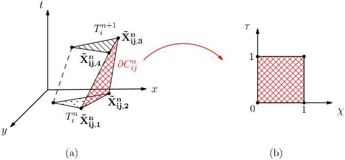
Figure 2: Physical space–time element (a) and parametrization of the lateral space–time subsurface $\partial C_{ij}^{n}$ (b).

The determinant of the coordinate transformation and the resulting space–time unit normal vector $\mathbf{\tilde{n}}_{ij}$ of the sub–surface $\partial C_{ij}^{n}$ can be computed as follows:

$$|\partial C_{ij}^{n}|=\left|\frac{\partial\mathbf{\tilde{x}}}{\partial\chi}\times\frac{\partial\mathbf{\tilde{x}}}{\partial\tau}\right|,\quad\mathbf{\tilde{n}}_{ij}=\left(\frac{\partial\mathbf{\tilde{x}}}{\partial\chi}\times\frac{\partial\mathbf{\tilde{x}}}{\partial\tau}\right)/|\partial C_{ij}^{n}|.$$ (48)

Note that the integration over a closed space–time volume as defined above automatically satisfies the geometric conservation law (GCL), since from the Gauss theorem follows

$$\int_{\partial\mathcal{C}_{i}^{n}}\mathbf{\tilde{n}}\,dS=0.$$ (49)

In all numerical simulations shown later in this paper, it has been confirmed for all time steps and all elements that the above relation (49) was always satisfied on the discrete level up to machine precision.

The final high order ALE one–step finite volume scheme takes the following form:

$$|T_{i}^{n+1}|\,\mathbf{Q}_{i}^{n+1}=|T_{i}^{n}|\,\mathbf{Q}_{i}^{n}-\sum\limits_{T_{j}\in\mathcal{N}_{i}}\,\,{\int\limits_{0}^{1}\int\limits_{0}^{1}|\partial C_{ij}^{n}|\tilde{\mathbf{G}}_{ij}\,d\chi d\tau}+\int\limits_{\mathcal{C}_{i}^{n}\backslash\partial\mathcal{C}_{i}^{n}}\left(\mathbf{S}_{h}-\mathbf{P}_{h}\right)\,d\mathbf{x}dt,$$ (50)

where the term $\tilde{\mathbf{G}}_{ij}\cdot\mathbf{\tilde{n}}_{ij}$ contains the Arbitrary–Lagrangian–Eulerian numerical flux function as well as the path–conservative jump term $\tilde{\mathbf{D}}$, to resolve the discontinuity of the predictor solution $\mathbf{q}_{h}$ at the space–time sub–face $\partial C_{ij}^{n}$. The surface integrals appearing in (50) are approximated using multidimensional Gaussian quadrature rules, see [126] for details. At the interface $\partial C_{ij}^{n}$ let us denote the local space–time predictor solution inside element $T_{i}(t)$ by $\mathbf{q}_{h}^{-}$ and the element–local predictor solution of the neighbor element $T_{j}(t)$ by $\mathbf{q}_{h}^{+}$, then a simple Rusanov–type scheme [56] is given by

$$\tilde{\mathbf{G}}_{ij}=\frac{1}{2}\left(\tilde{\mathbf{F}}(\mathbf{q}_{h}^{+})+\tilde{\mathbf{F}}(\mathbf{q}_{h}^{-})\right)\cdot\mathbf{\tilde{n}}_{ij}+\frac{1}{2}\left(\int\limits_{0}^{1}\tilde{\mathbf{B}}(\boldsymbol{\Psi})\cdot\mathbf{\tilde{n}}\ ds-|\lambda_{\max}|\mathbf{I}\right)\left(\mathbf{q}_{h}^{+}-\mathbf{q}_{h}^{-}\right)$$ (51)

where $|\lambda_{\max}|$ is the maximum absolute value of the eigenvalues of the matrix $\tilde{\mathbf{A}}\cdot\mathbf{\tilde{n}}$ in space–time normal direction, which can be expressed in terms of the classical Eulerian system matrix $\mathbf{A}=\partial\mathbf{F}/\partial\mathbf{Q}+\mathbf{B}$ and the normal mesh velocity $\mathbf{V}\cdot\mathbf{n}$ as

$$\tilde{\mathbf{A}}_{\mathbf{\tilde{n}}}=\tilde{\mathbf{A}}\cdot\mathbf{\tilde{n}}=\left(\sqrt{\tilde{n}_{x}^{2}+\tilde{n}_{y}^{2}}\,\right)\left[\left(\frac{\partial\mathbf{F}}{\partial\mathbf{Q}}+\mathbf{B}\right)\cdot\mathbf{n}-(\mathbf{V}\cdot\mathbf{n})\,\mathbf{I}\right],$$ (52)

with

$$\mathbf{n}=\frac{(\tilde{n}_{x},\tilde{n}_{y})^{T}}{\sqrt{\tilde{n}_{x}^{2}+\tilde{n}_{y}^{2}}}.$$ (53)

As stated above, $\mathbf{V}\cdot\mathbf{n}$ is the local normal mesh velocity and $\mathbf{I}$ is the $\nu\times\nu$ identity matrix. It can be easily verified that

$$\mathbf{V}=\frac{1}{\Delta t}\left(\begin{array}[]{c}x_{\tau}\\ y_{\tau}\end{array}\right),\quad\mathbf{\tilde{n}}_{ij}=\left(\begin{array}[]{c}\phantom{-}y_{\chi}\Delta t\\ -x_{\chi}\Delta t\\ x_{\chi}y_{\tau}-y_{\chi}x_{\tau}\end{array}\right),\quad\textnormal{ hence }\quad\mathbf{V}\cdot\mathbf{n}=-\frac{\tilde{n}_{t}}{\sqrt{\tilde{n}_{x}^{2}+\tilde{n}_{y}^{2}}}.$$ (54)

A more sophisticated Osher–type scheme [110] has been introduced in the Eulerian framework for conservative and for non–conservative hyperbolic systems in [54, 55]. It has been extended to the Lagrangian framework in one space dimension in [56] and reads in the general multi–dimensional case with conservative and non–conservative terms as follows:

$$\tilde{\mathbf{G}}_{ij}=\frac{1}{2}\left(\tilde{\mathbf{F}}(\mathbf{q}_{h}^{+})+\tilde{\mathbf{F}}(\mathbf{q}_{h}^{-})\right)\cdot\mathbf{\tilde{n}}_{ij}+\frac{1}{2}\left(\int\limits_{0}^{1}\left(\tilde{\mathbf{B}}(\boldsymbol{\Psi})\cdot\mathbf{\tilde{n}}-\left|\tilde{\mathbf{A}}_{\mathbf{\tilde{n}}}(\boldsymbol{\Psi})\right|\right)\,ds\,\right)\left(\mathbf{q}_{h}^{+}-\mathbf{q}_{h}^{-}\right),$$ (55)

In (55) above, the usual definition of the matrix absolute value operator applies, i.e.

$$|\mathbf{A}|=\mathbf{R}|\boldsymbol{\Lambda}|\mathbf{R}^{-1},\qquad|\boldsymbol{\Lambda}|=\textnormal{diag}\left(|\lambda_{1}|,|\lambda_{2}|,...,|\lambda_{\nu}|\right),$$ (56)

with the right eigenvector matrix $\mathbf{R}$ and its inverse $\mathbf{R}^{-1}$. According to [55, 54] the path integral appearing in (55) is approximated using Gaussian quadrature rules of sufficient accuracy.

2.4 Numerical Convergence Studies

In this section a numerical convergence study is performed for the compressible Baer–Nunziato model (1) in two space dimensions. This test problem has been proposed in [51] and has also been used in [55]. The test problem is similar to the one described in [76] and [8]. The exact solution of this smooth unsteady test problem is obtained in two steps: First, an exact stationary and rotationally symmetric solution of the governing PDE is sought and then the problem is made unsteady by superimposing a constant, uniform velocity field $\mathbf{\bar{v}}$ using the principle of Galilean invariance of Newtonian mechanics. The exact solution is then simply given by the advection of the nontrivial initial condition with the superimposed constant velocity field $\mathbf{\bar{v}}$. The rotationally symmetric solution is found by writing the governing equations (1) in polar coordinates ($r-\beta$) and by imposing angular symmetry $\partial/\partial\beta=0$. What remains is an ODE system in the radial coordinate $r$ that can be solved analytically, see [51].

In the following we denote with $u^{\beta}_{k}$ the angular velocities and with $u^{r}_{k}$ the radial velocities. Since we are interested in a vortex–type solution, we furthermore suppose that $u^{r}_{k}=0$. From the radial momentum equations we then obtain the following ODE system:

$$\begin{array}[]{ccc}\frac{\partial}{\partial r}\left(\phi_{1}p_{1}\right)&=&p_{2}\frac{\partial}{\partial r}\phi_{1}+\frac{1}{r}\left(u^{\beta}_{1}\right)^{2}\phi_{1}\rho_{1},\\ \frac{\partial}{\partial r}\left(\phi_{2}p_{2}\right)&=&p_{2}\frac{\partial}{\partial r}\phi_{2}+\frac{1}{r}\left(u^{\beta}_{2}\right)^{2}\phi_{2}\rho_{2}.\end{array}$$ (57)

If $\phi_{1}$, $p_{1}$ and $p_{2}$ are know, e.g. by simply prescribing them, then (57) is just a simple algebraic equation system for the angular velocities $u^{\beta}_{k}$. As in [51] we choose

$$p_{k}=p_{k0}\left(1-\frac{1}{4}e^{\displaystyle{\left(1-r^{2}/s_{k}^{2}\right)}}\right),\qquad(k=1,2)\;,$$ (58)

and

$$\phi_{1}=\frac{1}{3}+\frac{1}{2\sqrt{2\pi}}e^{\displaystyle{-r^{2}/2}},$$ (59)

hence the angular velocities of each phase result as

$$\begin{array}[]{l}u_{1}^{\theta}=\displaystyle{\frac{1}{2s_{1}D}}\sqrt{rD\left[p_{10}\left(4\sqrt{2\pi}F_{1}+6H_{1}-12Gs_{1}^{2}+3H_{1}s_{1}^{2}\right)+3p_{20}s_{1}^{2}\left(4G-H_{2}\right)\right]}\;,\\ \\ u_{2}^{\theta}=\displaystyle{\frac{r\sqrt{2}}{2\rho_{2}s_{2}}}\sqrt{\rho_{2}p_{20}F_{2}}\;,\end{array}$$ (60)

with the auxiliary variables

$$H_{k}=e^{\displaystyle{-\frac{2r^{2}+r^{2}s_{k}^{2}-2s_{k}^{2}}{2s_{k}^{2}}}},\quad F_{k}=e^{\displaystyle{-\frac{(r-s_{k})(r+s_{k})}{s_{k}^{2}}}},\quad(k=1,2),$$

and

$$G=e^{{-{r^{2}}/{2}}},\qquad D=\rho_{1}\left(2\sqrt{2\pi}+3G\right).$$

To this steady, rotationally symmetric solution of the compressible Baer-Nunziato equations we now add a constant uniform velocity field $\mathbf{\bar{v}}=(\bar{u},\bar{v})$ to make the test problem unsteady, as already mentioned above. This can be done since Newtonian mechanics is Galilean invariant. With this manufactured analytical solution we can now calculate the convergence rates of the new class of high order Lagrangian one–step WENO finite volume schemes presented previously in this section. For the computational setup, we use the following parameters:

$$\gamma_{1}=1.4,\quad\gamma_{2}=1.35,\quad\pi_{1}=\pi_{2}=0,\quad\bar{u}=\bar{v}=2,\quad\nu=\lambda=0,$$

$$\rho_{1}=1,\quad\rho_{2}=2,\quad p_{10}=1,\quad p_{20}=\frac{3}{2},\quad s_{1}=\frac{3}{2},\quad s_{2}=\frac{7}{5}.$$ (61)

The problem is solved with the Osher–type scheme (55) on a square domain $\Omega=[-10;10]\times[-10;10]$, using unstructured triangular meshes with four periodic boundary conditions, see Fig. 3, and setting the mesh velocity to $\mathbf{V}=\mathbf{u}_{I}=\mathbf{u}_{1}$. The numerical convergence rates are shown for the solid volume fraction $\phi_{s}$ at time $t=2.0$ in Table 1. One observes that the schemes reach their designed order of accuracy quite well. To our knowledge, this is the first time ever that a better than second order accurate Lagrangian WENO finite volume scheme is presented for non–conservative hyperbolic systems on unstructured triangular meshes with applications to the Baer–Nunziato model of compressible multi–phase flows.

Table 1: Numerical convergence results for the compressible Baer–Nunziato model using the third to sixth order version of the Arbitrary–Lagrangian–Eulerian one–step WENO finite volume schemes presented in this article. The error norms refer to the variable $\phi_{s}$ (solid volume fraction) at time $t=2.0$.

$N_{G}$	$\epsilon_{L_{2}}$	$\mathcal{O}(L_{2})$	$N_{G}$	$\epsilon_{L_{2}}$	$\mathcal{O}(L_{2})$
$\mathcal{O}3$			$\mathcal{O}4$
24	2.6916E-02	-	24	1.5993E-02	-
32	1.0906E-02	3.1	32	3.8281E-03	5.0
64	1.9750E-03	2.5	64	3.0900E-04	3.6
128	2.5442E-04	3.0	128	2.0855E-05	3.9
$\mathcal{O}5$			$\mathcal{O}6$
24	1.4493E-02	-	24	8.3869E-03	-
32	3.8912E-03	4.6	32	1.9504E-03	5.1
64	2.5564E-04	3.9	64	6.1843E-05	5.0
128	8.7457E-06	4.9	96	7.4509E-06	5.2

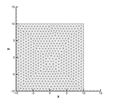
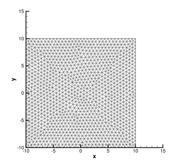
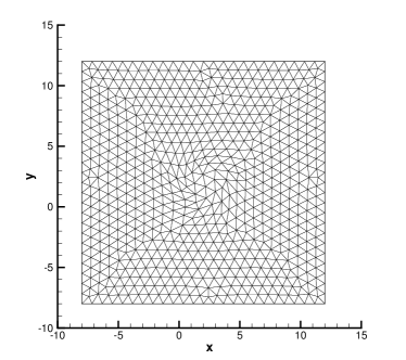
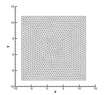
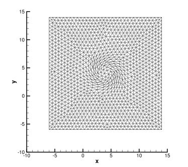
Figure 3: Moving Lagrangian meshes used for the numerical convergence test at times $t=0$ (top), $t=1$ (center) and $t=2$ (bottom) with resolution $24\times 24$ (left) and $32\times 32$ (right).

3 Test Problems

All the subsequent test problems are solved using the Osher–type method (55) and using the interface velocity, i.e. the solid velocity, as mesh velocity, hence $\mathbf{V}=\mathbf{u}_{I}=\mathbf{u}_{1}$. The CFL number in all test problems is set to $\textnormal{CFL}=0.5$. For all test problems we use a third order WENO scheme with reconstruction in characteristic variables [53] since componentwise reconstruction in conservative variables led to significant spurious oscillations. In all cases shown below, friction and pressure relaxation are neglected, hence ($\lambda=\nu=0$).

3.1 Riemann Problems

The high order finite volume ALE schemes proposed in this article are subsequently validated by applying them to 1D Riemann problems that are solved in a 2D geometry on unstructured triangular meshes. The exact solution for these 1D Riemann problems can be found in [5, 120, 39]. From the above mentioned articles we have chosen a subset of four Riemann problems, whose initial conditions are listed in Table 2. Some of the test cases use the stiffened gas EOS, some of them consider just a mixture of two ideal gases.

The initial two–dimensional computational domain is given by $\Omega(0)=[-0.5;0.5]\times[-0.05;0.05]$, which is discretized using an initial characteristic mesh spacing of $h=1/200$, corresponding to an equivalent one-dimensional resolution of 200 cells. The initial discontinuity is located at $x=0$ and the final simulation times are listed in Table 2. In $x$-direction we use transmissive boundaries and in $y$-direction periodic boundary conditions are imposed.

The numerical results are shown in Figs. 4 - 7 and are compared with the exact solution. On the top left of each figure a sketch of the mesh is depicted, while the other subfigures contain a one–dimensional cut through the reconstructed numerical solution $\mathbf{w}_{h}$ along the $x$-axis, evaluated at the final time on 200 equidistant sample points. Due to the Lagrangian formulation of the method, the solid contact is resolved in a very sharp manner in all cases, which was actually the main aim in the design of a high order Lagrangian–type scheme for the compressible Baer–Nunziato model. Also for the other waves we can note in general a very good agreement between our numerical results and the exact reference solutions given in [5, 120, 39], apart for RP3, where a visible misfit between the exact solution and numerical solution is obtained for the gas pressure and the gas density. However, even a very diffusive central path–conservative FORCE scheme in the Eulerian framework [51] had difficulties with this test problem and produced visible spurious oscillations and a wrong position of the solid contact in the gas phase. Further investigations on this problem are necessary, in particular, whether a different choice of the path is able to improve the situation.

Table 2: Initial states left (L) and right (R) for the Riemann problems solved in 2D and 3D with the Baer-Nunziato model. Values for $\gamma_{i}$, $\pi_{i}$ and the final time $t_{e}$ are also given.

	$\rho_{s}$	$u_{s}$	$p_{s}$	$\rho_{g}$	$u_{g}$	$p_{g}$	$\phi_{s}$	$t_{e}$
RP1 [39]:	$\gamma_{s}=1.4,\quad\pi_{s}=0,\quad\gamma_{g}=1.4,\quad\pi_{g}=0$
L	1.0	0.0	1.0	0.5	0.0	1.0	0.4	0.10
R	2.0	0.0	2.0	1.5	0.0	2.0	0.8
RP2 [39]:	$\gamma_{s}=3.0,\quad\pi_{s}=100,\quad\gamma_{g}=1.4,\quad\pi_{g}=0$
L	800.0	0.0	500.0	1.5	0.0	2.0	0.4	0.10
R	1000.0	0.0	600.0	1.0	0.0	1.0	0.3
RP3 [39]:	$\gamma_{s}=1.4,\quad\pi_{s}=0,\quad\gamma_{g}=1.4,\quad\pi_{g}=0$
L	1.0	0.9	2.5	1.0	0.0	1.0	0.9	0.10
R	1.0	0.0	1.0	1.2	1.0	2.0	0.2
RP4 [120]:	$\gamma_{s}=3.0,\quad\pi_{s}=3400,\quad\gamma_{g}=1.35,\quad\pi_{g}=0$
L	1900.0	0.0	10.0	2.0	0.0	3.0	0.2	0.15
R	1950.0	0.0	1000.0	1.0	0.0	1.0	0.9

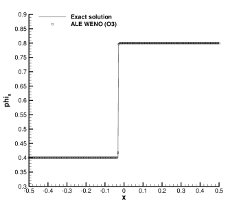
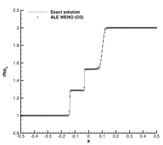
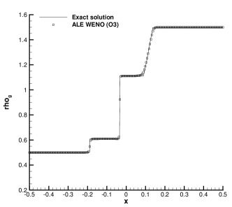
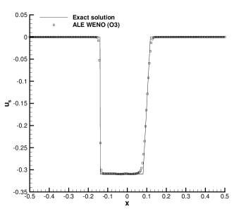
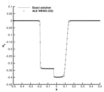
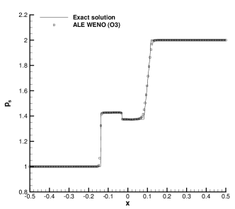
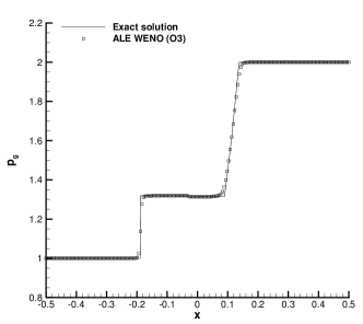
Figure 4: Results for Riemann problem RP1 of the seven-equation Baer-Nunziato model at time $t=0.1$.

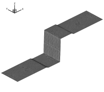
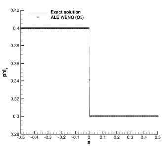
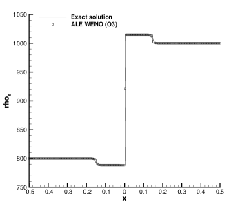
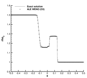
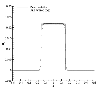
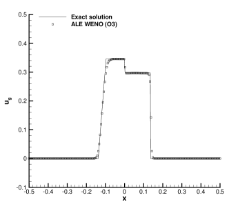
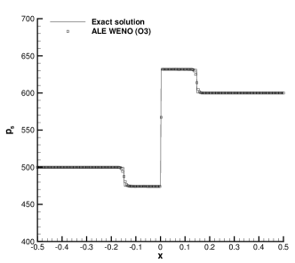
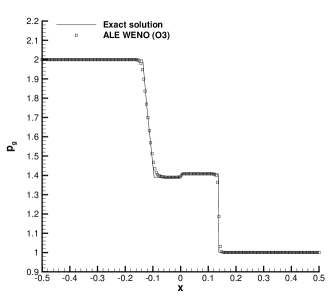
Figure 5: Results for Riemann problem RP2 of the seven-equation Baer-Nunziato model at time $t=0.1$.

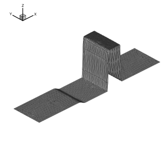
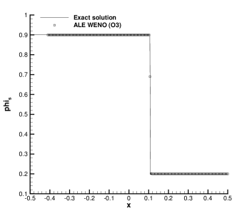
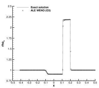
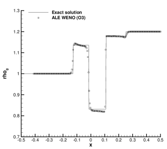
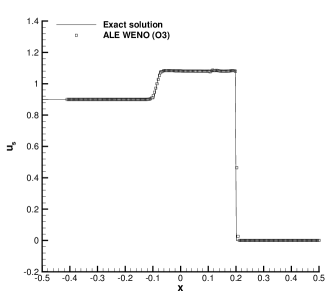
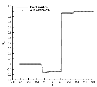
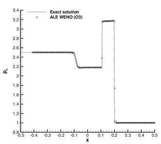
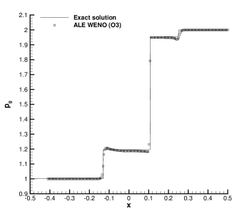
Figure 6: Results for Riemann problem RP3 of the seven-equation Baer-Nunziato model at time $t=0.1$.

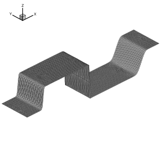
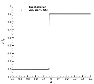
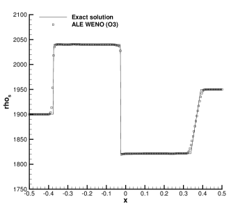
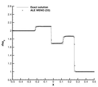
Figure 7: Results for Riemann problem RP4 of the seven-equation Baer-Nunziato model at time $t=0.15$.

3.2 Cylindrical Explosion Problems

Here we solve the compressible Baer–Nunziato equations in two space dimensions on a circular domain $\Omega(t)$ with initial radius $R=1.0$. The initial condition is in all cases given by

$$\mathbf{Q}(\mathbf{x},0)=\left\{\begin{array}[]{ll}\mathbf{Q}_{i},&\qquad\textnormal{ if }\quad|\mathbf{x}|<0.5,\\ \mathbf{Q}_{o},&\qquad\textnormal{ else.}\end{array}\right.$$ (62)

The reference solution is obtained by solving an equivalent non-conservative one-dimensional PDE in radial direction with geometric reaction source terms, see [130] for the Euler equations and [131] for the Baer–Nunziato model for details. In our case here the reference solution has been obtained by using an Eulerian second order TVD scheme on a very fine 1D mesh consisting of 10,000 cells. The initial conditions for the three explosion problems solved here are taken from the Riemann problems solved previously, where the left state is used as inner state and the right state is used as the outer state in (62), respectively. In particular, the first explosion problem EP1 uses the initial condition of RP1, EP2 corresponds to RP2 and EP3 to RP4, respectively. Also the parameters for the equation of state are chosen according to Table 2. The initial mesh spacing is of characteristic size $h=1/250$, leading to a total number of 431,224 triangular elements used to discretize $\Omega(t)$. The numerical results are compared with the 1D reference solution in Figures 8 - 10. On the top left of each figure a 3D visualization of either the solid or the gas density is shown, in order to verify that the cylindrical symmetry is reasonably maintained on the unstructured triangular meshes used here. The other subfigures show a one–dimensional cut through the reconstructed numerical solution $\mathbf{w}_{h}$ on 250 equidistant sample points along the $x$-axis. In all cases an excellent agreement between numerical solution and reference solution is obtained. Note, in particular, the very sharp resolution of the solid contact due to the use of a Lagrangian framework.

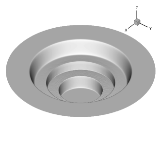
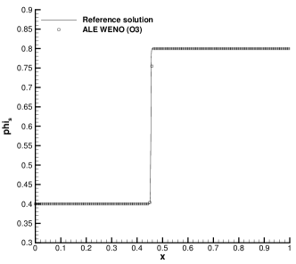
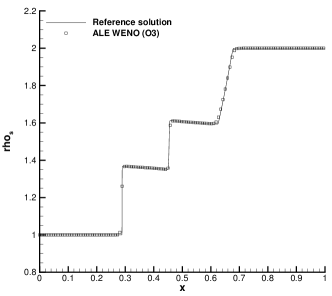
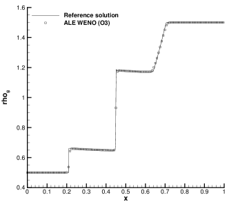
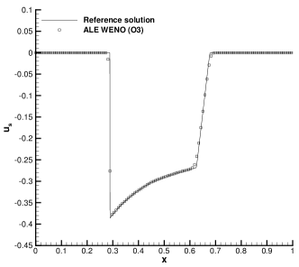
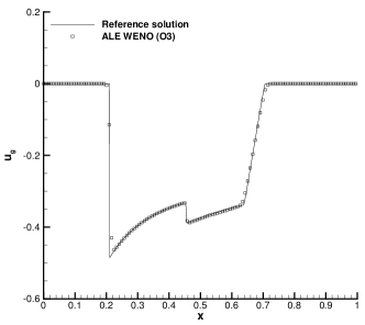
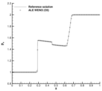
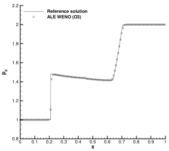
Figure 8: Results obtained for the first cylindrical explosion problem EP1 at $t=0.15$ and comparison with the reference solution.

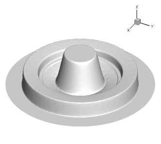
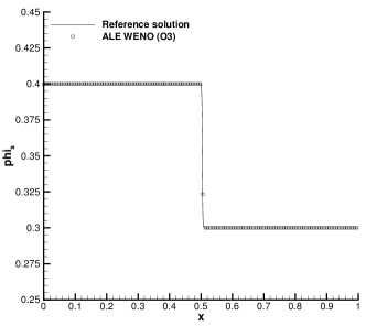
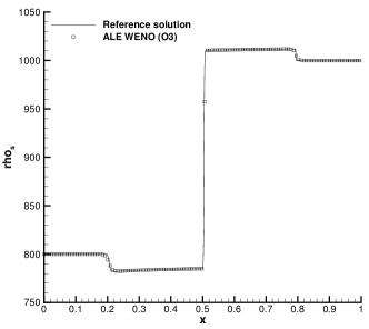
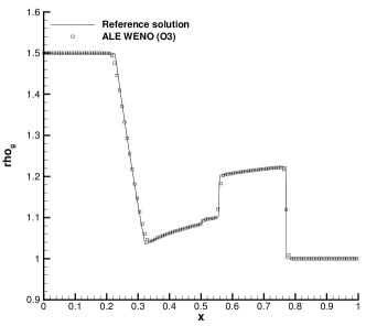
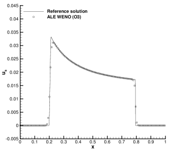
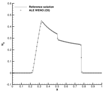
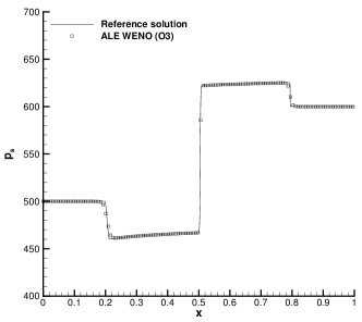
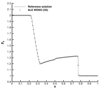
Figure 9: Results obtained for the first cylindrical explosion problem EP2 at $t=0.15$ and comparison with the reference solution.

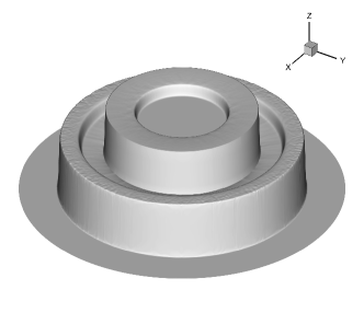
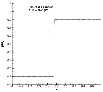
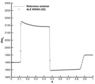
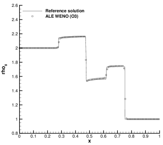
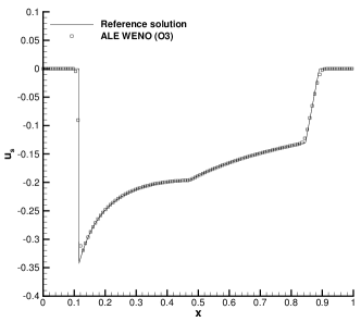
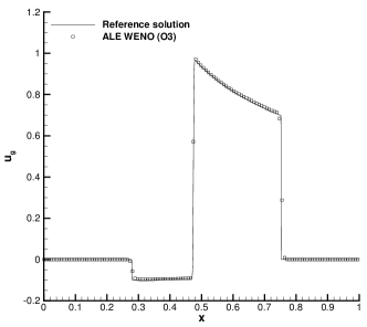
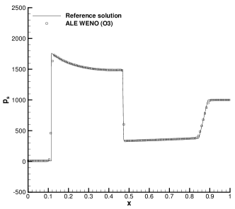
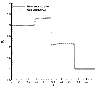
Figure 10: Results obtained for the first cylindrical explosion problem EP3 at $t=0.15$ and comparison with the reference solution.

3.3 Two–Dimensional Riemann Problems

In [83] Kurganov and Tadmor have collected a very nice set of numerical solutions for two–dimensional Riemann problems of the compressible Euler equations. Here, we propose an extension of these 2D Riemann problems to the compressible Baer–Nunziato model. The initial computational domain is $\Omega(0)=[-0.5;0.5]\times[-0.5;0.5]$ and the initial condition is given by four piecewise constant states defined in each quadrant of the two–dimensional coordinate system:

$$\mathbf{Q}(x,0)=\left\{\begin{array}[]{ccc}\mathbf{Q}_{1}&\textnormal{ if }&x>0\wedge y>0,\\ \mathbf{Q}_{2}&\textnormal{ if }&x\leq 0\wedge y>0,\\ \mathbf{Q}_{3}&\textnormal{ if }&x\leq 0\wedge y\leq 0,\\ \mathbf{Q}_{4}&\textnormal{ if }&x>0\wedge y\leq 0.\end{array}\right.$$ (63)

The initial conditions for the two configurations presented in this article are listed in Table 3. The simulations are carried out with a third order one–step ALE WENO finite volume scheme using an unstructured triangular mesh composed of 90,080 elements with an initial characteristic mesh spacing of $h=1/200$. The reference solution is computed with a high order Eulerian one–step scheme as presented in [131, 55], using a very fine mesh composed of 2,277,668 triangles with characteristic mesh spacing $h=1/1000$. Reflective wall boundaries are applied on the four boundaries of the domain. The obtained results together with the Eulerian reference solution are depicted in Figures 12 - 13, where we can note a very good qualitative agreement of the Lagrangian solution with the Eulerian fine–grid reference solution. For the first test problem, the initial and the final mesh are depicted in Fig. 11.

Table 3: Initial conditions for the two–dimensional Riemann problems.

Configuration C1 ($\gamma_{s}=1.4,\gamma_{g}=1.4,\pi_{s}=\pi_{g}=0$)
	$\rho_{s}$	$u_{s}$	$v_{s}$	$p_{s}$	$\rho_{g}$	$u_{g}$	$v_{g}$	$p_{g}$	$\phi_{s}$
$\mathbf{Q}_{1}:\,\,(x>0,y>0)$	2.0	0.0	0.0	2.0	1.5	0.0	0.0	2.0	0.8
$\mathbf{Q}_{2}:\,\,(x<0,y>0)$	1.0	0.0	0.0	1.0	0.5	0.0	0.0	1.0	0.4
$\mathbf{Q}_{3}:\,\,(x<0,y<0)$	2.0	0.0	0.0	2.0	1.5	0.0	0.0	2.0	0.8
$\mathbf{Q}_{4}:\,\,(x>0,y<0)$	1.0	0.0	0.0	1.0	0.5	0.0	0.0	1.0	0.4
Configuration C2 ($\gamma_{s}=3.0,\gamma_{g}=1.4,\pi_{s}=100,\pi_{g}=0$)
	$\rho_{s}$	$u_{s}$	$v_{s}$	$p_{s}$	$\rho_{g}$	$u_{g}$	$v_{g}$	$p_{g}$	$\phi_{s}$
$\mathbf{Q}_{1}:\,\,(x>0,y>0)$	1000.	0.0	0.0	600.0	1.0	0.0	0.0	1.0	0.3
$\mathbf{Q}_{2}:\,\,(x<0,y>0)$	800.	0.0	0.0	500.0	1.5	0.0	0.0	2.0	0.4
$\mathbf{Q}_{3}:\,\,(x<0,y<0)$	1000.	0.0	0.0	600.0	1.0	0.0	0.0	1.0	0.3
$\mathbf{Q}_{4}:\,\,(x>0,y<0)$	800.	0.0	0.0	500.0	1.5	0.0	0.0	2.0	0.4

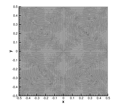
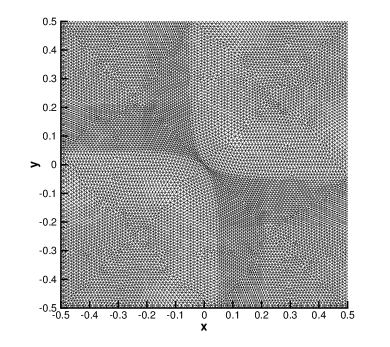
Figure 11: Mesh for configuration C1 at times $t=0$ (left) and $t=0.15$ (right).

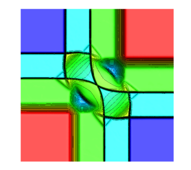
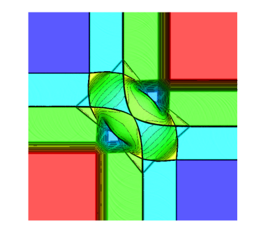
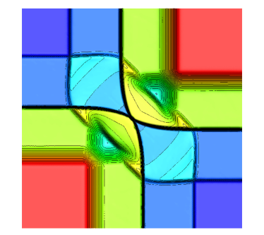
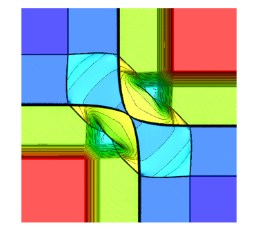
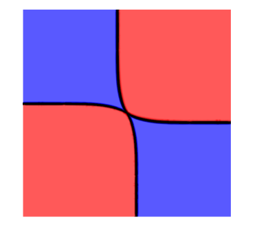
Figure 12: Results obtained with the third order Lagrangian WENO scheme for the 2D Riemann problem C1 at time $t=0.15$ (left column). The reference solution computed with an Eulerian method on a very fine mesh is also shown (right column). 30 equidistant contour lines are shown for the solid density $\rho_{s}$ (top row), the gas density $\rho_{g}$ (middle row) and the solid volume fraction $\phi_{s}$ (bottom row).

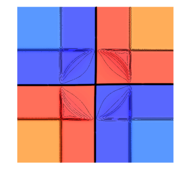
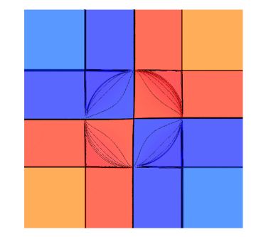
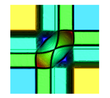
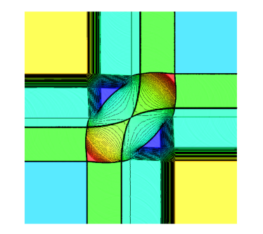
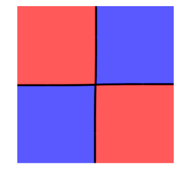
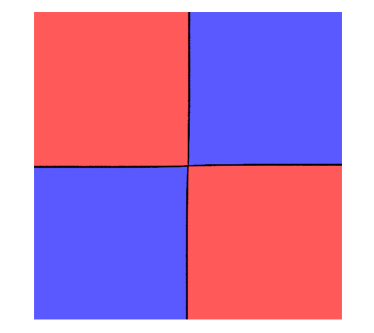
Figure 13: Results obtained with the third order Lagrangian WENO scheme for the 2D Riemann problem C2 at time $t=0.15$ (left column). The reference solution computed with an Eulerian method on a very fine mesh is also shown (right column). 30 equidistant contour lines are shown for the solid density $\rho_{s}$ (top row), the gas density $\rho_{g}$ (middle row) and the solid volume fraction $\phi_{s}$ (bottom row).

4 Application to Free Surface Flows with Moving Boundaries

4.1 Reduced Three–Equation Baer–Nunziato Model

The Baer–Nunziato model (1) considered in this paper can also be applied to complex non–hydrostatic free surface flows simulations, as proposed in [46, 44]. There, a reduced three–equation Baer–Nunziato model has been considered, which can be derived from the complete seven–equation model (1) by introducing three assumptions: firstly, all pressures are assumed to be relative pressures with respect to the atmospheric reference pressure, which is set to zero, i.e. $p_{0}:=0$; secondly, the gas phase that surrounds the liquid is supposed to remain always at atmospheric reference conditions, hence obtaining $p_{2}=p_{0}=0$, which allows to neglect all evolution equations related to the gas phase; finally, the pressure of the liquid phase is computed by the Tait equation of state [13], which reads

$$p_{1}=k_{0}\left[\left(\frac{\rho_{1}}{\rho_{0}}\right)^{\gamma}-1\right],$$ (64)

where $\rho_{1},\rho_{0}$ are the liquid density and the reference liquid density at standard conditions, respectively, $k_{0}$ is a constant that governs the compressibility of the fluid and $\gamma$ is a parameter commonly used to fit the equation of state with experimental data. Regarding the Tait equation (64), we should set the proper constant values for water, i.e. $k_{0}=3.2\cdot 10^{8}$ $Pa$, $\rho_{0}=1000$ $kg/m^{3}$ and $\gamma=7$, so that the typical speed of sound in water ($c=1500$ $m/s$) is preserved. However, since for most environmental free surface flows the maximum velocity is around $10$ $m/s$, or even less, we would have to deal with extremely low Mach numbers of $M=|\mathbf{u}|/c\ll 1$ that would cause very low time stepping and excessive numerical dissipation. In order to avoid this problem, we set artificially the Mach number to $M=0.3$, as done in [46, 44], and therefore we admit density fluctuations of the order of $10\%$. The advantage of using a weakly compressible model for free surface flows is the possibility to simulate environmental–type free surface flows as well as high speed industrial free surface flows, such as they appear in water jet cutting machines or fuel injection systems. There, speeds may reach up to $|\mathbf{u}|\approx 1000$ m/s and thus compressibility effects can no longer be neglected in the liquid.

By using the above mentioned simplifications and introducing them into system (1), as outlined in [46, 44], one can write the reduced Baer-Nunziato model as

$$\frac{\partial}{\partial t}\left(\phi\rho\right)+\nabla\cdot\left(\phi\rho\mathbf{u}\right)=0,$$ (65)

$$\frac{\partial}{\partial t}\left(\phi\rho\mathbf{u}\right)+\nabla\cdot\left(\phi\left(\rho\mathbf{u}\mathbf{u}+\boldsymbol{\sigma}\right)\right)=\phi\rho\mathbf{g},$$

$$\frac{\partial}{\partial t}\phi+\mathbf{u}\cdot\nabla\phi=0,$$

with the stress tensor $\boldsymbol{\sigma}=p\mathbf{I}$ of the inviscid liquid phase, for which we have dropped the subscript $1$ to ease notation. Mass and momentum equations are fully conservative in the system above, while the advection equation for the volume fraction is non–conservative. An evolution equation for total energy is not required, since we have used the assumption of a polytropic equation of state, which prescribes pressure as a function of density only. In (65) the state vector is $\mathbf{Q}=\left(\phi\rho,\phi\rho\mathbf{u},\phi\right)$ and $\mathbf{g}$ is the gravity vector acting along the vertical direction $y$, i.e. $\mathbf{g}=(0,g)$ with $g=9.81$ $m/s^{2}$. Further details on the derivation and on the assumptions of the reduced Baer–Nunziato model as well as a thorough validation against analytical solutions and experimental measurements can be found in [46, 44]. The system (65) above involves a compressible inviscid phase, without viscous effects. However, viscosity plays an important role in turbulent flows with violent free surface motion and therefore the algorithm can be improved and extended by adding the viscous terms to the stress tensor $\boldsymbol{\sigma}$ of the momentum equation in (65). The stress tensor of a Newtonian fluid using the hypothesis of Stokes reads

$$\boldsymbol{\sigma}=\left(p+\frac{2}{3}\mu\nabla\cdot\mathbf{u}\right)\mathbf{I}-\mu\left(\nabla\mathbf{u}+\nabla\mathbf{u}^{T}\right).$$ (66)

Here, $\mu$ denotes the dynamic viscosity, which for water is normally set to $10^{-3}$ $N\cdot s/m^{2}$. The discretization of the above model (65), which now also contains the viscous effects, is done according to [45, 48, 72] and can be directly inserted into the high order one–step approach used in this paper.

4.2 Sloshing in a Moving Tank

We apply the reduced Baer–Nunziato model with viscosity (65) to a well known free surface flow problem in moving geometries, namely to the sloshing motion of a liquid in a partially filled closed tank. Such a problem can not be described by the commonly used shallow water equations, since non–hydrostatic effects cannot be neglected. Furthermore, a numerical method is required that is able to deal with moving geometries, such as the present high order ALE finite volume scheme. The flow is rather complex, characterized by the presence of high amplitude oscillations and, eventually, also wave breaking may occur. Since our algorithm is designed to be an Arbitrary Lagrangian–Eulerian (ALE) scheme, for the present problem we decide to move the mesh according to the motion of the sloshing tank, which is prescribed on the boundary of the domain $\partial\Omega(t)$. Inside the domain $\Omega(t)$, the vertices are displaced smoothly according to the Laplace equation. In this case the evolution of the mesh and in particular the computation of the mesh velocity vector $\mathbf{V}(\mathbf{x},t)$ is governed by the following system of elliptic PDE:

$$\nabla^{2}\mathbf{V}(t)=0,\qquad\mathbf{V}(t)=\mathbf{V}_{\!D}(t)\quad\textnormal{for}\quad\mathbf{x}\in\partial\Omega(t),$$ (67)

which is solved in each time step and where the prescribed domain motion $\mathbf{V}_{\!D}(t)$ is imposed as Dirichlet boundary condition. The solution is obtained using a classical P1 finite element method (FEM), where the unknowns are located at the grid nodes and the solution of the discretized system (67) is computed by the conjugate gradient method. In this section the fluid motion and the mesh motion are governed by two different and independent laws, namely by the governing PDE system (65) and the Laplace equation (67), respectively. By solving (67) one obtains the velocity vector $\mathbf{V}$ for each grid vertex, which allows us to move the mesh nodes and to evolve the geometry, i.e. to compute all the other geometric quantities needed for the computation (normal vectors, element volumes, side lengths, barycenter positions, etc. ). From the solution of (67) the space–time control volumes needed for the local space–time Galerkin predictor and the final one–step finite volume scheme are known a priori.

The motion of liquid sloshing is a classical and widely investigated problem, since it occurs in many real world conditions whenever a sway tank is present, as in cargo ships, in liquid tank carriages on rail roads or in propellant tanks of rockets and airplanes engines. Sloshing phenomena have gained recent attention in coastal and offshore engineering with the proliferation of liquefied natural gas (LNG) and oil carriers transporting liquids in partially filled tanks [139], in order to assure and guarantee the safety of the sea transport of those fuels. The liquid sloshing motion can become very complex, even including wave breaking phenomena that can create highly localized impact pressure on tank walls, hence causing structural damages and affecting the stability of the vehicle which carries the container. Sloshing phenomena have been widely and intensively investigated in the last decades, focusing on the development of an analytical study based on the potential flow theory, as done by Faltinsen [57], who derived a linear analytical solution for liquid sloshing in a horizontally excited two–dimensional rectangular tank. Faltinsen and Timokha [59] extend the previous work to the nonlinear sloshing case and Hill [73] analyzed more in detail the waves’ behavior by relaxing some of the simplifications introduced in the previous studies. Also laboratory measurements of wave height and hydrodynamic pressure have been collected and reported [135, 104, 105, 4], which are very useful to validate both, theoretical solutions and numerical results. The theoretical analyses are however not suitable to describe real fluid sloshing, where viscosity and turbulence occur, so that a lot of research has been carried out in order to develop numerical models. In [57] Faltinsen developed a boundary element method (BEM), while Nakayama and Washizu [103] analyzed the non-linear liquid sloshing in a two–dimensional rectangular tank under pitch excitation by using the finite element method (FEM). Wu et al. [137] were the first who conducted a series of three–dimensional demonstrations on liquid sloshing based on FEM, but they did not compare the results to any experimental data. Another numerical technique is given by the finite difference method (FDM) with the use of coordinate transformations, as proposed by Chen et al. [31], who adopted a curvilinear coordinate system to map the sloshing from the non-rectangular physical domain into a rectangular computational domain. One can also solve the Navier–Stokes equations for viscous liquid sloshing [29, 28, 30] or the Reynolds Averaged Navier–Stokes equations (RANS) as proposed by Armenio et al. [6], who observed that the RANS model provides much more accurate results than the classical shallow water equations (SWE). For liquid sloshing the vertical acceleration is indeed very important and can not be neglected. In literature one can also find Lagrangian algorithms for sloshing phenomena, see the work of Okamoto et al. [104, 105], who were the first to apply an Arbitrary Lagrangian–Eulerian finite element method to two– and three–dimensional liquid sloshing, and also meshless Lagrangian particle methods, such as smoothed particle hydrodynamics (SPH) algorithms are used, as proposed in [122]. Multi–fluid sloshing has been studied with the Particle Finite Element Method (PFEM) in [79].

From the above mentioned references we know that the intensity and the impact of sloshing do generally depend on the amplitude and the frequency of the tank motion, on the physical properties of the fluid and on the geometry of the tank, i.e. its shape. Furthermore, liquid sloshing occurs when a tank is partially filled with fluid, so that a free surface is present. Very frequently high Reynolds numbers are achieved in such phenomena, therefore turbulence is usually present in this kind of flows. We improve indeed the algorithm by adding the simple zero-equation Smagorinsky turbulence model [123], which gives an expression for the eddy viscosity $\mu_{T}$ that is assumed to be proportional to the velocity gradients. For the two–dimensional case the Smagorinsky model reads

$$\mu_{T}=\rho\cdot\left(C_{S}\Delta\right)^{2}|\overline{\mathbf{S}}|,$$ (68)

where $C_{S}$ is a coefficient which has to be set properly, $\Delta$ is the turbulence length scale and the term $|\overline{\mathbf{S}}|$ is given by

$$|\overline{\mathbf{S}}|=\sqrt{2\overline{S_{ij}}\overline{S_{ij}}},\qquad\overline{S_{ij}}=\frac{1}{2}\left(\frac{\partial u_{i}}{\partial x_{j}}+\frac{\partial u_{j}}{\partial x_{i}}\right),$$ (69)

with the strain rate tensor $\overline{S_{ij}}$. The Smagorninsky constant is usually in the range $\left[0.1;0.24\right]$ and here we set $C_{S}=0.17$. In this paper show numerical results for an idealized two–dimensional case, where the tank is moving with a purely horizontal sinusoidal velocity and the vertical velocity component is zero, i.e.

$$\mathbf{V}_{\!D}(t)=\left(V_{A}\sin\left(\omega t\right),0\right)^{T}$$ (70)

where $\omega=\frac{2\pi}{T}$ is the frequency of the oscillation and $T$ is the period, while $V_{A}$ quantifies the amplitude of the sinusoidal velocity, which is related to the horizontal tank displacement $\delta x_{A}$ by $V_{A}=-\omega\delta x_{A}$. We always assume the fluid and the tank to be initially at rest, i.e. $\mathbf{V}(0)=0$.

The simulations presented in this paper refer to the very recent work of Shao et al. [122], who present an improved SPH method for modeling liquid sloshing dynamics. Their main novelty regards the use of the Reynolds averaged turbulence model incorporated into the SPH method in order to properly describe the effects of turbulence. Furthermore, in [122] some new density and kernel gradient corrections have been introduced to achieve better accuracy and smoother pressure fields. The initial domain $\Omega(0)$ refers to the one used for the laboratory measurements carried out by Faltinsen et al. [58] and is represented by a two–dimensional rectangular tank of dimensions $\Omega(0)=[0;1.73]\times[0;1.15]$, as sketched in Figure 14. We use an unstructured triangular mesh with a total number of $N_{e}=44746$ elements.

Figure 14: Sloshing tank.

The lateral sides and the bottom of the domain are modelled by classical no–slip wall boundary conditions for viscous flow, while the above boundary is set as transmissive outflow. The computational domain is characterized by a periodic excitation along the horizontal direction $x$, whose displacement $\delta x(t)$ is described as $\delta x(t)=\delta x_{A}\cdot\cos(\omega t)$, where we fix the parameters $\delta x_{A}=0.032$ and $T=1.3$ with the initial water height $h_{w}=0.6$, as proposed in [122]. The corresponding velocity law for the tank can be easily computed by (70), with $V_{A}=-\omega\delta x_{A}$. In this case we are dealing with a turbulent flow, since the Reynolds number $Re=\frac{L\cdot u}{\nu}$ is of the order of $10^{6}$. Regarding the parameters of the equation of state (64), we set $k_{0}=8.5\cdot 10^{4}$ $Pa$, $\rho_{0}=1000$ $kg/m^{3}$ and $\gamma=1$, as suggested in [46, 44].

Figure 15 shows a comparison between experimental data and numerical results: the periodic motion of the tank can be clearly identified looking at the perturbation $H$ of the free surface location with respect to the initial configuration. The numerical results have been collected at the same probe point $\mathbf{x}_{p}$ used for the experimental data, which is placed on the initial free surface level and is $0.05$ $m$ away from the left wall, hence its initial location is $\mathbf{x}_{p}(0)=(0.05,0.6)$. Since the probe point is attached to the tank, it moves together with the domain. Furthermore the value of $H$ is evaluated at each time step as

$$H=\int\limits_{h_{\Omega}}\phi(s)ds-h_{w},\qquad\textnormal{ with }\qquad h_{\Omega}\in[0,1.15]$$ (71)

where the volume fraction integral along the whole height $h_{\Omega}$ of the domain represents indeed the water column at the probe point which is shifting horizontally according to Eqn.(70) and $h_{w}$ is the initial free surface elevation. As the tank motion begins, water moves towards the left, hence decreasing the pressure ($t=0.5$), then the tank changes completely direction shifting towards the right side and therefore the free surface elevation increases its level up to $0.7$ $m$ at time $t=1.2$ $s$. The water keeps moving following the described periodic cycle of the tank boundaries, progressively increasing the wave amplitude in time. The numerical results are in good agreement with the experimental data, also with the particular wiggles observed in the time interval $t\in[5;7]s$, see Fig. 15.

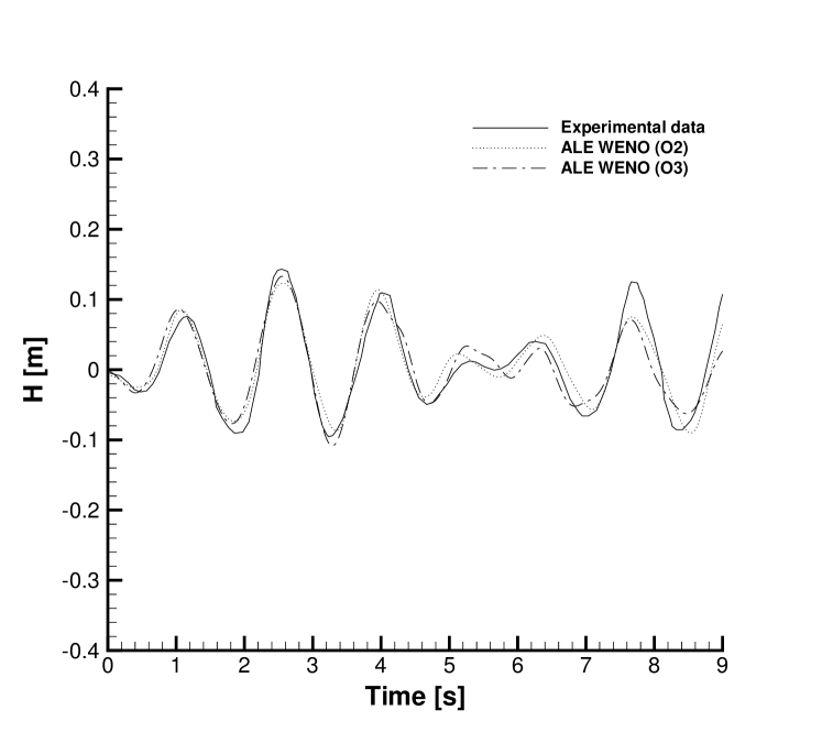
Figure 15: Sloshing motion: comparison between experimental data (solid line), second order (dotted line) and third order ALE WENO scheme (dash-dot line). $T=1.3$ $s$ and $h_{w}=0.6$ $m$.

Another comparison of numerical results with experimental data is depicted in Figure 16 for two different sets of parameters: on the left we show the case $T=1.5s$ and $h_{w}=0.6m$, while on the right we use $T=1.875s$ and $h_{w}=0.5m$.

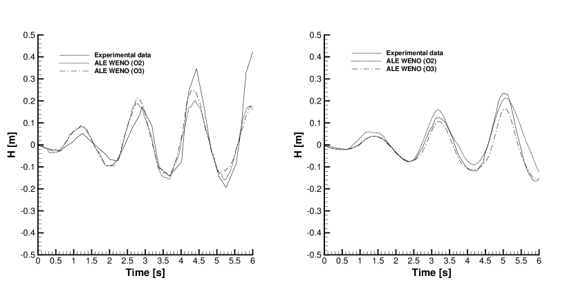
Figure 16: Comparison between experimental data (solid line) and numerical results with second (dotted line) and third (dash-dot line) order of accuracy. Left: $T=1.5$ $h_{w}=0.5$. Right: $T=1.875$ $h_{w}=0.5$.

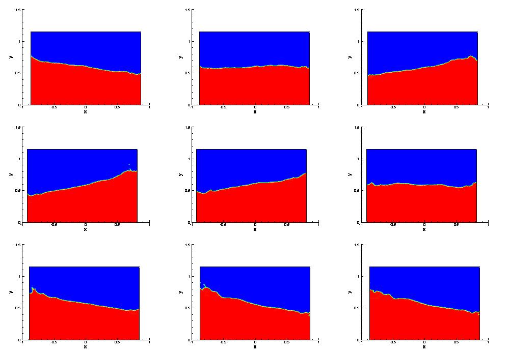
Figure 17: Water motion for the case $T=1.5s$ and $h_{w}=0.6m$ at times $t=3.0$, $3.2$, $3.4$, $3.6$, $3.8$, $4.0$, $4.2$, $4.4$ and $4.5$ $s$.

The flow pattern of the sloshing for $T=1.5s$ and $h_{w}=0.6m$ is plotted in Figure 17 at nine representative time instants within one period. One can notice the strong oscillations of the free surface occurring in the flow while the tank is swinging, as well as the motion of the domain $\Omega(t)$.

5 Conclusions

In this article the first better than second order Arbitrary–Lagrangian-Eulerian one–step WENO finite volume scheme on unstructured triangular meshes has been proposed for the solution of hyperbolic systems with non–conservative products. The method has been applied to the full seven equation Baer–Nunziato model of compressible multiphase flows as well as to a reduced three–equation model for the simulation of weakly compressible free surface flows in moving geometries. High order of accuracy in space and time have been verified by a numerical convergence study on a smooth unsteady test problem where an exact solution of the Baer–Nunziato model is available. The scheme has also been successfully applied to problems with shock waves and material interfaces. For all test problems the numerical results have been compared with exact or numerical reference solutions in order to validate the approach.

In future research we plan to extend the present scheme to three space dimensions in the more general framework of the new $P_{N}P_{M}$ method proposed in [47], which unifies high order finite volume and discontinuous Galerkin finite element methods in one general approach. Further work will also consist in a generalization to moving curved meshes as well as the introduction of multi–dimensional Riemann solvers, such as the ones used in [90, 10, 11]. Finally, more research is necessary concerning a suitable conservative and high order accurate remapping / remeshing strategy to deal with significant mesh distorsions arising in the presence of strong shear waves.

References

- [1] R. Abgrall. On essentially non-oscillatory schemes on unstructured meshes: analysis and implementation. Journal of Computational Physics, 144:45–58, 1994.
- [2] R. Abgrall and S. Karni. A comment on the computation of non-conservative products. Journal of Computational Physics, 229:2759–2763, 2010.
- [3] T. Aboiyar, E.H. Georgoulis, and A. Iske. Adaptive ADER Methods Using Kernel-Based Polyharmonic Spline WENO Reconstruction. SIAM Journal on Scientific Computing, 32:3251–3277, 2010.
- [4] H. Akyildiz and E. Unal. Experimental investigation of pressure distribution on a rectangular tank due to the liquid sloshing. Ocean Eng., 32:1503 – 1516, 2005.
- [5] N. Andrianov and G. Warnecke. The Riemann problem for the Baer–Nunziato two-phase flow model. Journal of Computational Physics, 212:434–464, 2004.
- [6] V. Armenio and M. La Rocca. On the analysis of sloshing of water in rectangular containers: numerical and experimental investigation. Ocean Eng., 23:705 – 739, 1996.
- [7] M.R. Baer and J.W. Nunziato. A two-phase mixture theory for the deflagration-to-detonation transition (DDT) in reactive granular materials. J. Multiphase Flow, 12:861 –889, 1986.
- [8] D. Balsara. Second-order accurate schemes for magnetohydrodynamics with divergence-free reconstruction. The Astrophysical Journal Supplement Series, 151:149–184, 2004.
- [9] D. Balsara and C.W. Shu. Monotonicity preserving weighted essentially non-oscillatory schemes with increasingly high order of accuracy. Journal of Computational Physics, 160:405–452, 2000.
- [10] D.S. Balsara. Multidimensional HLLE Riemann solver: Application to Euler and magnetohydrodynamic flows. Journal of Computational Physics, 229:1970–1993, 2010.
- [11] D.S. Balsara. A two-dimensional HLLC Riemann solver for conservation laws: Application to Euler and magnetohydrodynamic flows. Journal of Computational Physics, 231:7476–7503, 2012.
- [12] T.J. Barth and P.O. Frederickson. Higher order solution of the Euler equations on unstructured grids using quadratic reconstruction. AIAA paper no. 90-0013, 28th Aerospace Sciences Meeting January 1990.
- [13] G. K. Batchelor. An Introduction to Fluid Mechanics. Cambridge University Press, 1974.
- [14] D.J. Benson. Computational methods in lagrangian and eulerian hydrocodes. Computer Methods in Applied Mechanics and Engineering, 99:235–394, 1992.
- [15] M. Berndt, J. Breil, S. Galera, M. Kucharik, P.H. Maire, and M. Shashkov. Two–step hybrid conservative remapping for multimaterial arbitrary Lagrangian -Eulerian methods. Journal of Computational Physics, 230:6664–6687, 2011.
- [16] W. Boscheri and M. Dumbser. Arbitrary–Lagrangian–Eulerian One–Step WENO Finite Volume Schemes on Unstructured Triangular Meshes. Communications in Computational Physics. submitted to.
- [17] W. Boscheri, M. Dumbser, and M. Righetti. A semi-implicit scheme for 3d free surface flows with high order velocity reconstruction on unstructured voronoi meshes. International Journal for Numerical Methods in Fluids. DOI: 10.1002/fld.3753, in press.
- [18] J. Breil, S. Galera, and P.H. Maire. Multi-material ALE computation in inertial confinement fusion code CHIC. Computers and Fluids, 46:161–167, 2011.
- [19] J. Breil, T. Harribey, P.H. Maire, and M. Shashkov. A multi-material ReALE method with MOF interface reconstruction. Computers and Fluids. DOI: 10.1016/j.compfluid.2012.08.015, in press.
- [20] E.J. Caramana, D.E. Burton, M.J. Shashkov, and P.P. Whalen. The construction of compatible hydrodynamics algorithms utilizing conservation of total energy. Journal of Computational Physics, 146:227–262, 1998.
- [21] G. Carré, S. Del Pino, B. Després, and E. Labourasse. A cell-centered lagrangian hydrodynamics scheme on general unstructured meshes in arbitrary dimension. Journal of Computational Physics, 228:5160 – 5183, 2009.
- [22] M.J. Castro, J.M. Gallardo, J.A. López, and C. Parés. Well-balanced high order extensions of godunov’s method for semilinear balance laws. SIAM Journal of Numerical Analysis, 46:1012–1039, 2008.
- [23] M.J. Castro, J.M. Gallardo, and C. Parés. High-order finite volume schemes based on reconstruction of states for solving hyperbolic systems with nonconservative products. applications to shallow-water systems. Mathematics of Computation, 75:1103– 1134, 2006.
- [24] M.J. Castro, P.G. LeFloch, M.L. Muñoz-Ruiz, and C. Parés. Why many theories of shock waves are necessary: Convergence error in formally path-consistent schemes. Journal of Computational Physics, 227:8107–8129, 2008.
- [25] V. Casulli. Semi-implicit finite difference methods for the two-dimensional shallow water equations. Journal of Computational Physics, 86:56–74, 1990.
- [26] V. Casulli and R.T. Cheng. Semi-implicit finite difference methods for three-dimensional shallow water flow. International Journal of Numerical Methods in Fluids, 15:629–648, 1992.
- [27] J. Cesenek, M. Feistauer, J. Horacek, V. Kucera, and J. Prokopova. Simulation of compressible viscous flow in time-dependent domains. Applied Mathematics and Computation. DOI: 10.1016/j.amc.2011.08.077, in press.
- [28] B. F. Chen. Viscous fluid in a tank under coupled surge, heave and pitch motions. J. Waterw. Port Coast. Ocean Eng.–ASCE, 131:239 – 256, 2005.
- [29] B. F. Chen and H. W. Chiang. Complete 2d and fully nonlinear analysis of ideal fluid in tanks. J. Eng. Mech.–ASCE, 125:70 – 78, 1999.
- [30] B. F. Chen and R. Nokes. Time–independent finite difference analysis of 2d and nonlinear viscous liquid sloshing in a rectangular tank. J. comput. Phys., 209:47 – 81, 2005.
- [31] W. Chen, M. A. Haroun, and F. Liu. Large amplitude liquid sloshing in seismically excited tanks. Earthquake Eng. Struct. Dyn., 25:653 – 669, 1996.
- [32] J. Cheng and C.W. Shu. A high order ENO conservative Lagrangian type scheme for the compressible Euler equations. Journal of Computational Physics, 227:1567–1596, 2007.
- [33] J. Cheng and C.W. Shu. A cell-centered Lagrangian scheme with the preservation of symmetry and conservation properties for compressible fluid flows in two-dimensional cylindrical geometry. Journal of Computational Physics, 229:7191–7206, 2010.
- [34] J. Cheng and C.W. Shu. Improvement on spherical symmetry in two-dimensional cylindrical coordinates for a class of control volume Lagrangian schemes. Communications in Computational Physics, 11:1144–1168, 2012.
- [35] S. Clain, S. Diot, and R. Loubère. A high–order finite volume method for systems of conservation laws – Multi–dimensional Optimal Order Detection (MOOD). Journal of Computational Physics, 230:4028–4050, 2011.
- [36] A. Claisse, B. Després, E.Labourasse, and F. Ledoux. A new exceptional points method with application to cell-centered lagrangian schemes and curved meshes. Journal of Computational Physics, 231:4324–4354, 2012.
- [37] B. Cockburn, G. E. Karniadakis, and C.W. Shu. Discontinuous Galerkin Methods. Lecture Notes in Computational Science and Engineering. Springer, 2000.
- [38] R. Courant, E. Isaacson, and M. Rees. On the solution of nonlinear hyperbolic differential equations by finite differences. Comm. Pure Appl. Math., 5:243–255, 1952.
- [39] V. Deledicque and M.V. Papalexandris. An exact Riemann solver for compressible two-phase flow models containing non-conservative products. Journal of Computational Physics, 222:217–245, 2007.
- [40] B. Després and C. Mazeran. Symmetrization of lagrangian gas dynamic in dimension two and multimdimensional solvers. C.R. Mecanique, 331:475–480, 2003.
- [41] B. Després and C. Mazeran. Lagrangian gas dynamics in two-dimensions and lagrangian systems. Archive for Rational Mechanics and Analysis, 178:327–372, 2005.
- [42] L. Dubcova, M. Feistauer, J. Horacek, and P. Svacek. Numerical simulation of interaction between turbulent flow and a vibrating airfoil. Computing and Visualization in Science, 12:207–225, 2009.
- [43] M. Dubiner. Spectral methods on triangles and other domains. Journal of Scientific Computing, 6:345–390, 1991.
- [44] M. Dumbser. A Diffuse Interface Method for Complex Three-Dimensional Free Surface Flows. Computer Methods in Applied Mechanics and Engineering. DOI: , in press.
- [45] M. Dumbser. Arbitrary high order PNPM schemes on unstructured meshes for the compressible Navier–Stokes equations. Computers & Fluids, 39:60–76, 2010.
- [46] M. Dumbser. A simple two-phase method for the simulation of complex free surface flows. Computer Methods in Applied Mechanics and Engineering, 200:1204– 1219, 2011.
- [47] M. Dumbser, D. Balsara, E.F. Toro, and C.D. Munz. A unified framework for the construction of one–step finite–volume and discontinuous Galerkin schemes. Journal of Computational Physics, 227:8209–8253, 2008.
- [48] M. Dumbser and D.S. Balsara. High–order unstructured one-step PNPM schemes for the viscous and resistive MHD equations. CMES - Computer Modeling in Engineering & Sciences, 54:301–333, 2009.
- [49] M. Dumbser, M. Castro, C. Parés, and E.F. Toro. ADER schemes on unstructured meshes for non-conservative hyperbolic systems: Applications to geophysical flows. Computers and Fluids, 38:1731– 1748, 2009.
- [50] M. Dumbser, C. Enaux, and E.F. Toro. Finite volume schemes of very high order of accuracy for stiff hyperbolic balance laws. Journal of Computational Physics, 227:3971–4001, 2008.
- [51] M. Dumbser, A. Hidalgo, M. Castro, C. Parés, and E.F. Toro. FORCE schemes on unstructured meshes II: Non–conservative hyperbolic systems. Computer Methods in Applied Mechanics and Engineering, 199:625–647, 2010.
- [52] M. Dumbser and M. Käser. Arbitrary high order non-oscillatory finite volume schemes on unstructured meshes for linear hyperbolic systems. Journal of Computational Physics, 221:693–723, 2007.
- [53] M. Dumbser, M. Käser, V.A Titarev, and E.F. Toro. Quadrature-free non-oscillatory finite volume schemes on unstructured meshes for nonlinear hyperbolic systems. Journal of Computational Physics, 226:204–243, 2007.
- [54] M. Dumbser and E. F. Toro. On universal Osher–type schemes for general nonlinear hyperbolic conservation laws. Communications in Computational Physics, 10:635–671, 2011.
- [55] M. Dumbser and E. F. Toro. A simple extension of the Osher Riemann solver to non-conservative hyperbolic systems. Journal of Scientific Computing, 48:70–88, 2011.
- [56] M. Dumbser, A. Uuriintsetseg, and O. Zanotti. On Arbitrary–Lagrangian–Eulerian One–Step WENO Schemes for Stiff Hyperbolic Balance Laws. Communications in Computational Physics, 14:301–327, 2013.
- [57] O. M. Faltinsen. A numerical nonlinear method of sloshing in tanks with two–dimensional flow. J. Ship Res., 22:193 – 202, 1978.
- [58] O. M. Faltinsen, O. F. Rognebakke, and I. A. Lukovsky nd A. N. Timokha. Adaptive multimodal approach to nonlinear sloshing in a rectangular tank. J. Fluid Mech., 407:201 – 234, 2000.
- [59] O. M. Faltinsen and A. N. Timokha. Adaptive multimodal approach to nonlinear sloshing in a rectangular tank. J. Fluid Mech., 432:167 – 200, 2001.
- [60] R. Fedkiw, T. Aslam, B. Merriman, and S. Osher. A non-oscillatory Eulerian approach to interfaces in multimaterial flows (the ghost fluid method). Journal of Computational Physics, 152:457–492, 1999.
- [61] R.P. Fedkiw, T. Aslam, and S. Xu. The Ghost Fluid method for deflagration and detonation discontinuities. Journal of Computational Physics, 154:393–427, 1999.
- [62] M. Feistauer, J. Horacek, M. Ruzicka, and P. Svacek. Numerical analysis of flow-induced nonlinear vibrations of an airfoil with three degrees of freedom. Computers and Fluids, 49:110–127, 2011.
- [63] M. Feistauer, V. Kucera, J. Prokopova, and J. Horacek. The ALE discontinuous Galerkin method for the simulatio of air flow through pulsating human vocal folds. AIP Conference Proceedings, 1281:83–86, 2010.
- [64] A. Ferrari, M. Dumbser, E.F. Toro, and A. Armanini. A New Stable Version of the SPH Method in Lagrangian Coordinates. Communications in Computational Physics, 4:378–404, 2008.
- [65] A. Ferrari, M. Dumbser, E.F. Toro, and A. Armanini. A new 3D parallel SPH scheme for free surface flows. Computers & Fluids, 38:1203–1217, 2009.
- [66] A. Ferrari, L. Fraccarollo, M. Dumbser, E.F. Toro, and A. Armanini. Three–dimensional flow evolution after a dambreak. Journal of Fluid Mechanics, 663:456–477, 2010.
- [67] A. Ferrari, C.D. Munz, and B. Weigand. A high order sharp interface method with local timestepping for compressible multiphase flows. Communications in Computational Physics, 9:205–230, 2011.
- [68] O. Friedrich. Weighted essentially non-oscillatory schemes for the interpolation of mean values on unstructured grids. Journal of Computational Physics, 144:194–212, 1998.
- [69] G. Gassner, M. Dumbser, F. Hindenlang, and C.D. Munz. Explicit one–step time discretizations for discontinuous Galerkin and finite volume schemes based on local predictors. Journal of Computational Physics, 230:4232–4247, 2011.
- [70] A. Harten, B. Engquist, S. Osher, and S. Chakravarthy. Uniformly high order essentially non-oscillatory schemes, III. Journal of Computational Physics, 71:231–303, 1987.
- [71] R.W. Healy and T.F. Russel. Solution of the advection-dispersion equation in two dimensions by a finite-volume eulerian-lagrangian localized adjoint method. Advances in Water Resources, 21:11–26, 1998.
- [72] A. Hidalgo and M. Dumbser. ADER schemes for nonlinear systems of stiff advection diffusion reaction equations. Journal of Scientific Computing, 48:173–189, 2011.
- [73] D. F. Hill. Transient and steady–state amplitudes of forced waves in rectangular basins. Phys. Fluid, 15:1576 – 1587, 2003.
- [74] C. Hirt, A. Amsden, and J. Cook. An arbitrary lagrangian eulerian computing method for all flow speeds. Journal of Computational Physics, 14:227 253, 1974.
- [75] C. W. Hirt and B. D. Nichols. Volume of fluid (VOF) method for dynamics of free boundaries. Journal of Computational Physics, 39:201–225, 1981.
- [76] C. Hu and C.W. Shu. Weighted essentially non-oscillatory schemes on triangular meshes. Journal of Computational Physics, 150:97–127, 1999.
- [77] C.S. Huang, T. Arbogast, and J. Qiu. An eulerian-lagrangian weno finite volume scheme for advection problems. Journal of Computational Physics, 231:4028–4052, 2012.
- [78] S. R. Idelsohn, E. Oñate, and F. Del Pin. The Particle Finite Element Method: a powerful tool to solve incompressible flows with free-surfaces and breaking waves. International Journal for Numerical Methods in Engineering, 61:964–984, 2004.
- [79] S.R. Idelsohn, M. Mier-Torrecilla, and E. Oñate. Multi–fluid flows with the Particle Finite Element Method. Comput. Methods Appl. Mech. Engrg., 198:2750–2767, 2009.
- [80] G.S. Jiang and C.W. Shu. Efficient implementation of weighted ENO schemes. Journal of Computational Physics, 126:202–228, 1996.
- [81] G. E. Karniadakis and S. J. Sherwin. Spectral/hp Element Methods in CFD. Oxford University Press, 1999.
- [82] M. Käser and A. Iske. ADER schemes on adaptive triangular meshes for scalar conservation laws. Journal of Computational Physics, 205:486–508, 2005.
- [83] A. Kurganov and E. Tadmor. Solution of two-dimensional Riemann problems for gas dynamics without Riemann problem solvers. Numer. Methods Partial Differential Equations, 18:584–608, 2002.
- [84] A. Larese, R. Rossi, E. Oñate, and S.R. Idelsohn. Validation of the Particle Finite Element Method (PFEM) for Simulation of the Free-Surface Flows. Engineering Computations, 25:385–425, 2008.
- [85] P.D. Lax and B. Wendroff. Systems of conservation laws. Communications in Pure and Applied Mathematics, 13:217–237, 1960.
- [86] M. Lentine, Jón Tómas Grétarsson, and R. Fedkiw. An unconditionally stable fully conservative semi-lagrangian method. Journal of Computational Physics, 230:2857–2879, 2011.
- [87] W. Liu, J. Cheng, and C.W. Shu. High order conservative Lagrangian schemes with Lax Wendroff type time discretization for the compressible Euler equations. Journal of Computational Physics, 228:8872–8891, 2009.
- [88] R. Löhner, C. Yang, and E. Onate. On the simulation of flows with violent free surface motion. Computer Methods in Applied Mechanics and Engineering, 195:5597–5620, 2006.
- [89] R. Loubère, P.H. Maire, and M. Shashkov. ReALE: A Reconnection Arbitrary–Lagrangian -Eulerian method in cylindrical geometry. Computers and Fluids, 46:59–69, 2011.
- [90] R. Loubère, P.H. Maire, and P. Váchal. A second–order compatible staggered Lagrangian hydrodynamics scheme using a cell–centered multidimensional approximate Riemann solver. Procedia Computer Science, 1:1931–1939, 2010.
- [91] P.-H. Maire. A high-order one-step sub-cell force-based discretization for cell-centered lagrangian hydrodynamics on polygonal grids. Computers and Fluids, 46(1):341–347, 2011.
- [92] P.-H. Maire. A unified sub-cell force-based discretization for cell-centered lagrangian hydrodynamics on polygonal grids. International Journal for Numerical Methods in Fluids, 65:1281 1294, 2011.
- [93] P.H. Maire. A high-order cell–centered Lagrangian scheme for compressible fluid flows in two–dimensional cylindrical geometry . Journal of Computational Physics, 228:6882–6915, 2009.
- [94] P.H. Maire. A high-order cell-centered lagrangian scheme for two-dimensional compressible fluid flows on unstructured meshes. Journal of Computational Physics, 228:2391 – 2425, 2009.
- [95] P.H. Maire, R. Abgrall, J. Breil, and J. Ovadia. A cell-centered lagrangian scheme for two-dimensional compressible flow problems. SIAM Journal on Scientific Computing, 29:1781 1824, 2007.
- [96] P.H. Maire and B. Nkonga. Multi-scale Godunov-type method for cell-centered discrete Lagrangian hydrodynamics. Journal of Computational Physics, 228:799–821, 2009.
- [97] G. Dal Maso, P.G. LeFloch, and F. Murat. Definition and weak stability of nonconservative products. J. Math. Pures Appl., 74:483 –548, 1995.
- [98] J.J. Monaghan. Simulating free surface flows with SPH. Journal of Computational Physics, 110:399–406, 1994.
- [99] M.L. Muñoz and C. Parés. Godunov method for nonconservative hyperbolic systems. Mathematical Modelling and Numerical Analysis, 41:169–185, 2007.
- [100] W. Mulder, S. Osher, and J.A. Sethian. Computing interface motion in compressible gas dynamics. Journal of Computational Physics, 100:209–228, 1992.
- [101] C.D. Munz. On Godunov–type schemes for Lagrangian gas dynamics. SIAM Journal on Numerical Analysis, 31:17–42, 1994.
- [102] A. Murrone and H. Guillard. A five equation reduced model for compressible two phase flow problems. Journal of Computational Physics, 202:664–698, 2005.
- [103] T. Nakayama and K. Washizu. Nonlinear analysis of liquid motion in a container subjected to forced pitching oscillation. Int. J. Numer. Method Eng., 15:1207 – 1220, 1980.
- [104] T. Okamoto and M. Kawahara. Two–dimensional sloshing analysis by lagrangian finite element method. Int. Numer. Method Fluid, 11:453 – 477, 1990.
- [105] T. Okamoto and M. Kawahara. 3d sloshing analysis by an arbitrary lagrangian -eulerian finite element method. Int. J. Comput. Fluid Dyn., 8:129 – 146, 1997.
- [106] E. Oñate, M. Celigueta, S. Idelsohn, F. Salazar, and B. Suarez. Possibilities of the Particle Finite Element Method for fluid–soil–structure interaction problems. Journal of Computational Mechanics, 48:307–318, 2011.
- [107] E. Oñate, S.R. Idelsohn, M.A. Celigueta, and R. Rossi. Advances in the Particle Finite Element Method for the Analysis of Fluid-Multibody Interaction and Bed Erosion in Free-surface Flows. Computer Methods in Applied Mechanics and Engineering, 197:1777–1800, 2008.
- [108] A. López Ortega and G. Scovazzi. A geometrically–conservative, synchronized, flux–corrected remap for arbitrary Lagrangian–Eulerian computations with nodal finite elements. Journal of Computational Physics, 230:6709–6741, 2011.
- [109] S. Osher and J.A. Sethian. Fronts propagating with curvature–dependent speed: Algorithms based on Hamilton–Jacobi formulations. Journal of Computational Physics, 79:12–49, 1988.
- [110] S. Osher and F. Solomon. Upwind difference schemes for hyperbolic conservation laws. Math. Comput., 38:339–374, 1982.
- [111] C. Parés. Numerical methods for nonconservative hyperbolic systems: a theoretical framework. SIAM Journal on Numerical Analysis, 44:300– 321, 2006.
- [112] C. Parés and M.J. Castro. On the well-balance property of roe’s method for nonconservative hyperbolic systems. applications to shallow-water systems. Mathematical Modelling and Numerical Analysis, 38:821–852, 2004.
- [113] J.S. Peery and D.E. Carroll. Multi-material ale methods in unstructured grids,. Computer Methods in Applied Mechanics and Engineering, 187:591–619, 2000.
- [114] F. Del Pin, S. R. Idelsohn, E. Oñate, and R. Aubry. The ALE/Lagrangian Particle Finite Element Method: A new approach to computation of free-surface flows and fluid-object interactions. Computers and Fluids, 36:27–38, 2007.
- [115] Jing-Mei Qiu and Chi-Wang Shu. Conservative high order semi-lagrangian finite difference weno methods for advection in incompressible flow. Journal of Computational Physics, 230:863–889, 2011.
- [116] S. Rhebergen, O. Bokhove, and J.J.W. van der Vegt. Discontinuous Galerkin finite element methods for hyperbolic nonconservative partial differential equations. Journal of Computational Physics, 227:1887– 1922, 2008.
- [117] M. Rieber and A. Frohn. A numerical study on the mechanism of splashing. International Journal of Heat and Fluid Flow, 20:455–461, 1999.
- [118] K. Riemslagh, J. Vierendeels, and E. Dick. An arbitrary lagrangian-eulerian finite-volume method for the simulation of rotary displaecment pump flow. Applied Numerical Mathematics, 32:419–433, 2000.
- [119] R. Saurel and R. Abgrall. A multiphase Godunov method for compressible multifluid and multiphase flows. Journal of Computational Physics, 150:425–467, 1999.
- [120] D.W. Schwendeman, C.W. Wahle, and A.K. Kapila. The Riemann problem and a high-resolution Godunov method for a model of compressible two-phase flow. Journal of Computational Physics, 212:490–526, 2006.
- [121] G. Scovazzi. Lagrangian shock hydrodynamics on tetrahedral meshes: A stable and accurate variational multiscale approach. Journal of Computational Physics, 231:8029–8069, 2012.
- [122] J. R. Shao, H. Q. Li, G. R. Liu, and M. B. Liu. An improved sph method for modeling liquid sloshing dynamics. Computers and Structures, 101:18 – 26, 2012.
- [123] S. Smagorinsky. General circulation experiments with the primitive equations. Mon. Weather Rev., 91:99 – 164, 1963.
- [124] R.W. Smith. AUSM(ALE): a geometrically conservative arbitrary lagrangian–eulerian flux splitting scheme. Journal of Computational Physics, 150:268 286, 1999.
- [125] T. Sonar. On the construction of essentially non-oscillatory finite volume approximations to hyperbolic conservation laws on general triangulations: polynomial recovery, accuracy and stencil selection. Computer Methods in Applied Mechanics and Engineering, 140:157–181, 1997.
- [126] A.H. Stroud. Approximate Calculation of Multiple Integrals. Prentice-Hall Inc., Englewood Cliffs, New Jersey, 1971.
- [127] B. Tian, E.F. Toro, and C.E. Castro. A path-conservative method for a five-equation model of two-phase flow with an hllc-type riemann solver. Computers and Fluids, 46:122–132, 2011.
- [128] V.A. Titarev, P. Tsoutsanis, and D. Drikakis. WENO schemes for mixed–element unstructured meshes. Communications in Computational Physics, 8:585–609, 2010.
- [129] S.A. Tokareva and E.F. Toro. Hllc–type riemann solver for the baer nunziato equations of compressible two-phase flow. Journal of Computational Physics, 229:3573–3604, 2010.
- [130] E.F. Toro. Riemann Solvers and Numerical Methods for Fluid Dynamics. Springer, second edition, 1999.
- [131] E.F. Toro, A. Hidalgo, and M. Dumbser. FORCE schemes on unstructured meshes I: Conservative hyperbolic systems. Journal of Computational Physics, 228:3368–3389, 2009.
- [132] I. Toumi. A weak formulation of Roe’s approximate Riemann solver. Journal of Computational Physics, 102:360–373, 1992.
- [133] P. Tsoutsanis, V.A. Titarev, and D. Drikakis. WENO schemes on arbitrary mixed-element unstructured meshes in three space dimensions. Journal of Computational Physics, 230:1585–1601, 2011.
- [134] B. van Leer. Towards the ultimate conservative difference scheme V: A second order sequel to Godunov’s method. Journal of Computational Physics, 32:101–136, 1979.
- [135] H. G. Verhagen and L. Wijingaarden. Nonlinear oscillation of fluid in a container. J. Fluid. Mech., 22:737 – 751, 1965.
- [136] J. von Neumann and R.D. Richtmyer. A method for the calculation of hydrodynamics shocks. Journal of Applied Physics, 21:232–237, 1950.
- [137] G. X. Wu, Q. A. Ma, and R. E. Taylor. Numerical simulation of sloshing waves in a 3d tank based on a finite element method. Appl. Ocean Res., 20:337 – 355, 1998.
- [138] Y.T. Zhang and C.W. Shu. Third order WENO scheme on three dimensional tetrahedral meshes. Communications in Computational Physics, 5:836–848, 2009.
- [139] W. Zhao, J. Yang, Z. Hu, and L. Xiao. Experimental investigation of effects of inner–tank sloshing on hydrodynamics of an FLNG system. Journal of Hydrodynamics, 24:107 – 115, 2012.