Functional integral approach to semi-relativistic Pauli-Fierz models

Abstract

By means of functional integrations spectral properties of semi-relativistic Pauli-Fierz Hamiltonians

$$H=\sqrt{({\rm p}-\alpha{\rm A})^{2}+m^{2}}-m+V+{\rm H}_{\rm rad}$$

in quantum electrodynamics is considered. Here ${\rm p}$ is the momentum operator, ${\rm A}$ a quantized radiation field on which an ultraviolet cutoff is imposed, $V$ an external potential, ${\rm H}_{\rm rad}$ the free field Hamiltonian and $m\geq 0$ describes the mass of electron. Two self-adjoint extensions of a semi-relativistic Pauli-Fierz Hamiltonian are defined. The Feynman-Kac type formula of $e^{-tH}$ is given. An essential self-adjointness, a spatial decay of bound states, a Gaussian domination of the ground state and the existence of a measure associated with the ground state are shown. All the results are independent of values of coupling constant $\alpha$, and it is emphasized that $m=0$ is included.

1 Introduction

1.1 Preliminary

In the past decade a great deal of work has been devoted to studying spectral properties of non-relativistic quantum electrodynamics in the purely mathematical point of view. In this paper we are concerned with the semi-relativistic Pauli-Fierz model (it is abbreviated as SRPF model) in quantum electrodynamics and its spectral properties by using functional integrations. The SRPF model describes a minimal interaction between semi-relativistic electrons and a massless quantized radiation field $A$ on which an ultraviolet cutoff function is imposed. We assume throughout this paper that the electron is spinless and moves in $d$ $(\geq 3)$ dimensional Euclidean space for simplicity. In the case where the electron has spin ${1/2}$, the procedure is similar and we shall publish details somewhere. A Hamiltonian of semi-relativistic as well as non-relativistic quantum electrodynamics is usually described as a self-adjoint operator in the tensor product of a Hilbert space and a boson Fock space. In this paper instead of the boson Fock space we can formulate the Hamiltonian as a self-adjoint operator in the known Schrödinger representation in a functional realization of the boson Fock space as a space of square integrable functions with respect to the corresponding Gaussian measure. Through the Schrödinger representation a Fyenman-Kac type formula of the strongly continuous one parameter semigroup generated by the SRPF Hamiltonian is given. A functional integral or a path measure approach is proven to be useful to study properties of bound states associated with embedded eigenvalues in the continuous spectrum. See e.g., [LHB11, Sections 6 and 7] . We are interested in investigating properties of bound states and ground states of the SRPF Hamiltonian by functional integrations.

1.2 Self-adjoint extensions and functional integrations

The SRPF Hamiltonian can be realized as a self-adjoint operator bounded from below in the tensor product of ${L^{2}({{\mathbb{R}}^{d}})}$ and a boson Fock space ${\mathscr{F}}$, where ${L^{2}({{\mathbb{R}}^{d}})}$ denotes the state space of a semi-relativistic electron and ${\mathscr{F}}$ that of photons. Then the decoupled Hamiltonian is given by

$$(\sqrt{{\rm p}^{2}+m^{2}}-m+V)\otimes{\mathchoice{\rm 1\mskip-4.0mul}{\rm 1\mskip-4.0mul}{\rm 1\mskip-4.5mul}{\rm 1\mskip-5.0mul}}+{\mathchoice{\rm 1\mskip-4.0mul}{\rm 1\mskip-4.0mul}{\rm 1\mskip-4.5mul}{\rm 1\mskip-5.0mul}}\otimes{\rm H}_{\rm rad},$$ (1.1)

where ${\rm p}=({\rm p}_{1},...,{\rm p}_{d})=(-i\partial_{x_{1}},...,-i\partial_{x_{d}})$ denotes the momentum operator, $m$ electron mass, $V:{{\mathbb{R}}^{d}}\to{\mathbb{R}}$ an external potntial, and ${\rm H}_{\rm rad}$ the free field Hamiltonian on ${\mathscr{F}}$. The SRPF Hamiltonian is defined by introducing the minimal coupling by the quantized radiation field $A$ with cutoff function ${\hat{\varphi}}$, i.e., replacing ${\rm p}\otimes{\mathchoice{\rm 1\mskip-4.0mul}{\rm 1\mskip-4.0mul}{\rm 1\mskip-4.5mul}{\rm 1\mskip-5.0mul}}$ with ${\rm p}\otimes{\mathchoice{\rm 1\mskip-4.0mul}{\rm 1\mskip-4.0mul}{\rm 1\mskip-4.5mul}{\rm 1\mskip-5.0mul}}-\alpha A$ and, then

$${\rm H}=\sqrt{({\rm p}\otimes{\mathchoice{\rm 1\mskip-4.0mul}{\rm 1\mskip-4.0mul}{\rm 1\mskip-4.5mul}{\rm 1\mskip-5.0mul}}-\alpha A)^{2}+m^{2}}-m+V\otimes{\mathchoice{\rm 1\mskip-4.0mul}{\rm 1\mskip-4.0mul}{\rm 1\mskip-4.5mul}{\rm 1\mskip-5.0mul}}+{\mathchoice{\rm 1\mskip-4.0mul}{\rm 1\mskip-4.0mul}{\rm 1\mskip-4.5mul}{\rm 1\mskip-5.0mul}}\otimes{\rm H}_{\rm rad},$$ (1.2)

where $\alpha$ is a real coupling constant. In order to investigate the semigroup ${\rm e}^{-t{\rm H}}$, $t\geq 0$, we redefine ${\rm H}$ on ${L^{2}({{\mathbb{R}}^{d}})}\otimes L^{2}({\mathscr{Q}})$ instead of ${L^{2}({{\mathbb{R}}^{d}})}\otimes{\mathscr{F}}$, where $L^{2}({\mathscr{Q}})$ denotes the set of square integrable functions on a Gaussian probability space $({\mathscr{Q}},\mu)$, and is called a Schrödinger representation of ${\mathscr{F}}$.

We introduce three classes, $\mathscr{V}_{\rm qf}$, $\mathscr{V}_{\rm Kato}$ and $\mathscr{V}_{\rm rel}$, of external potentials. The definitions of $\mathscr{V}_{\rm qf}$, $\mathscr{V}_{\rm Kato}$ and $\mathscr{V}_{\rm rel}$ are given in Definitions 3.13, 5.1, and 3.11, respectively. Note that $\mathscr{V}_{\rm Kato}$ contains relativistic Kato-class potentials (see (1.7)), $\mathscr{V}_{\rm rel}$ potentials being relatively bounded with respect to $\sqrt{{\rm p}^{2}+m^{2}}-m$, and $\mathscr{V}_{\rm Kato}\subset\mathscr{V}_{\rm qf}$, $\mathscr{V}_{\rm rel}\subset\mathscr{V}_{\rm qf}$ hold. We show in Theorems 4.5 and 4.7 that ${\rm H}$ is self-adjoint on $D(|{\rm p}|\otimes{\mathchoice{\rm 1\mskip-4.0mul}{\rm 1\mskip-4.0mul}{\rm 1\mskip-4.5mul}{\rm 1\mskip-5.0mul}})\cap D({\mathchoice{\rm 1\mskip-4.0mul}{\rm 1\mskip-4.0mul}{\rm 1\mskip-4.5mul}{\rm 1\mskip-5.0mul}}\otimes{\rm H}_{\rm rad})$ for $V\in\mathscr{V}_{\rm rel}$. For more singular potentials we shall construct two appropriate self-adjoint extensions of ${\rm H}$, which are denoted by ${\rm H}_{\rm qf}$ and ${\rm H}_{\rm K}$. The former is defined for $V\in\mathscr{V}_{\rm qf}$ by the quadratic form sum and the later for $V\in\mathscr{V}_{\rm Kato}$ through Feynman-Kac type formula. See Definition 3.13 for ${\rm H}_{\rm qf}$ and Definition 5.3 for ${\rm H}_{\rm K}$. Although $\mathscr{V}_{\rm qf}$ is wider than $\mathscr{V}_{\rm Kato}$, ${\rm H}_{\rm K}$ is defined under weaker condition on cutoff function ${\hat{\varphi}}$ than that for ${\rm H}_{\rm qf}$.

In Introduction ${\rm H}$ stands for ${\rm H}_{\rm qf}$ or ${\rm H}_{\rm K}$ in what follows. We construct the Feynman-Kac type formula of ${\rm e}^{-t{\rm H}}$ in terms of a composition of Euclidean quantum field ${\rm A}_{\rm E}(f)$ with test function $f\in{\mathscr{E}}=\bigoplus^{d}L_{\mathbb{R}}^{2}({{\mathbb{R}}^{d+1}})$, $d$-dimensional Brownian motion $(B_{t})_{t\in{\mathbb{R}}}$ on the whole real line ${\mathbb{R}}$ defined on a probability space $(\Omega_{\rm P},\mathscr{B}_{\rm P},{\rm P}^{x})$, and a subordinator $(T_{t})_{t\geq 0}$ on $(\Omega_{\nu},\mathscr{B}_{\nu},\nu)$. The Euclidean quantum field ${\rm A}_{\rm E}(f)$ is Gaussian, and the covariance is given by $\mathbb{E}_{\mu_{\rm E}}[{\rm A}_{\rm E}(f){\rm A}_{\rm E}(g)]={\rm q_{\rm E}}(f,g)$ with some bilinear form ${\rm q_{\rm E}}(\cdot,\cdot)$ on ${\mathscr{E}}\times{\mathscr{E}}$. Hence it is driven in Theorem 3.15 and Corollary 3.16 that

$$(F,{\rm e}^{-2t{\rm H}}G)=\int_{{\mathbb{R}}^{d}}\!\!\!\!{\rm d}x\mathbb{E}_{{\rm P}\!\times\!\nu}^{x,0}\!\left[\!\left(\!{\rm J}_{-t}F(B_{-T_{t}}),{\rm e}^{-i\alpha{\rm A}_{\rm E}({\rm I}[-t,t])}{\rm e}^{-\int_{-t}^{t}V(B_{T_{s}}){\rm d}s}{\rm J}_{t}G(B_{T_{t}})\!\right)\!\right]$$ (1.3)

for $F,G\in L^{2}({{\mathbb{R}}^{d}};L^{2}({\mathscr{Q}}))\cong{L^{2}({{\mathbb{R}}^{d}})}\otimes L^{2}({\mathscr{Q}})$. Here ${\rm I}[-t,t]$ is a limit of ${\mathscr{E}}$-valued stochastic integrals, which is formally written as

$${\rm I}[-t,t]=\bigoplus_{\mu=1}^{d}\int_{-T_{t}}^{T_{t}}{\rm j}_{T^{\ast}_{s}}\lambda(\cdot-B_{s})\!{\rm d}B_{s}^{\mu}$$ (1.4)

with $\lambda=({\hat{\varphi}}/\sqrt{\omega}\check{)}$. Here $T^{\ast}_{s}=\inf\{t|T_{t}=s\}$ is the first hitting time of $(T_{t})_{t\geq 0}$ at $s$. Notations ${\rm J}_{t}$ and ${\rm j}_{t}$ are defined in Section 2.2 below, and the rigorous definition of (1.4) is given in Lemma 3.7, Remarks 3.8 and 3.17.

1.3 Main results

By using the Feynman-Kac type formula (1.3) we study the spectrum of the SRPF Hamiltonian ${\rm H}$. The main results of this paper are (a)-(d) below:

(a)

Self-adjointness and essential self-adjointness of ${\rm H}$ (Theorems 4.5 and 4.7).

(b)

Spatial decay of bound states $\Phi_{\rm b}$ of ${\rm H}$ (Theorem 5.12).

(c)

Gaussian domination of the ground state $\varphi_{\rm g}$ of ${\rm H}$ (Theorem 6.8).

(d)

Existence of a probability measure $\mu_{\infty}$ associated with $\varphi_{\rm g}$ (Theorem 7.3).

The spectrum of non-relativistic versions of ${\rm H}$, which is the so-called Pauli-Fierz model, have been studied, and among other things the existence of a ground state is proven in [BFS99, GLL01]. See also [Spo04] and references therein. The spectrum of semi-relativistic versions, ${\rm H}$, is also studied in e.g., [FGS01, HH13a, HH13b, KMS09, KMS11, KMS12, MS10, MS09] from an operator-theoretic point of view. In particular the existence of ground states of ${\rm H}$ are considered under some conditions in [KMS09, KMS12] for $m>0$ and [HH13b] for $m\geq 0$.

Here are outlines of assertions (a)-(d) mentioned above.

(a) Following our previous work [Hir00b], we investigate (a). This can be proven by estimating the scalar product $|(KF,{\rm e}^{-t{\rm H}}G)|$ for self-adjoint operators $K={\mathchoice{\rm 1\mskip-4.0mul}{\rm 1\mskip-4.0mul}{\rm 1\mskip-4.5mul}{\rm 1\mskip-5.0mul}}\otimes{\rm H}_{\rm rad}$ and ${\rm p}_{\mu}\otimes{\mathchoice{\rm 1\mskip-4.0mul}{\rm 1\mskip-4.0mul}{\rm 1\mskip-4.5mul}{\rm 1\mskip-5.0mul}}$. Let $V=0$. Then a bound $|(KF,{\rm e}^{-t{\rm H}}G)|\leq C_{K,G}\|F\|$, $F,G\in{\rm D}({\rm H})$, is shown with some constant $C_{K,G}$. Hence ${\rm e}^{-t{\rm H}}$ leaves ${\rm D}(|{\rm p}|\otimes{\mathchoice{\rm 1\mskip-4.0mul}{\rm 1\mskip-4.0mul}{\rm 1\mskip-4.5mul}{\rm 1\mskip-5.0mul}})\cap{\rm D}({\mathchoice{\rm 1\mskip-4.0mul}{\rm 1\mskip-4.0mul}{\rm 1\mskip-4.5mul}{\rm 1\mskip-5.0mul}}\otimes{\rm H}_{\rm rad})$ invariant for $V=0$ and we can conclude that ${\rm H}$ is essentially self-adjoint on ${\rm D}(|{\rm p}|\otimes{\mathchoice{\rm 1\mskip-4.0mul}{\rm 1\mskip-4.0mul}{\rm 1\mskip-4.5mul}{\rm 1\mskip-5.0mul}})\cap{\rm D}({\mathchoice{\rm 1\mskip-4.0mul}{\rm 1\mskip-4.0mul}{\rm 1\mskip-4.5mul}{\rm 1\mskip-5.0mul}}\otimes{\rm H}_{\rm rad})$ by Proposition 3.3 for $V\in\mathscr{V}_{\rm rel}$ for arbitrary values of $\alpha$. This is an extension of that of a non-relativistic case established in [Hir00b] and [LHB11, Section 7.4.1]. Furthermore the self-adjointness of ${\rm H}$ is shown in Theorem 4.7. Examples include a spinless hydrogen like atom (Example 4.8). It is noted that our method is also available to the SRPF Hamiltonian with spin. We give a comment on known results. Although in [KMS11, MS10] the self-adjointness of the SRPF Hamiltonian with spin ${1/2}$ is considered, it is not sure that the method can be available to spinless cases.

(b) Let

$${\rm H}_{\rm p}=\sqrt{{\rm p}^{2}+m^{2}}-m+V$$ (1.5)

be the semi-relativistic Schrödinger operator. Let $(z_{t})_{t\geq 0}$ be the $d$-dimensional Lévy process on a probability space $(\Omega_{\rm Z},\mathscr{B}_{\rm Z},{\rm Z}^{x})$ such that $\mathbb{E}_{\rm Z}^{x}\left[\!{\rm e}^{-iu\cdot z_{t}}\!\right]={\rm e}^{-t(\sqrt{|u|^{2}+m^{2}}-m)}{\rm e}^{-iu\cdot x}$. Hence the self-adjoint generator of $(z_{t})_{t\geq 0}$ is given by $\sqrt{{\rm p}^{2}+m^{2}}-m$. The Feynman-Kac type formula for ${\rm H}_{\rm p}$ is thus given by

$$(f,{\rm e}^{-t{\rm H}_{\rm p}}g)=\int_{{\mathbb{R}}^{d}}\!{\rm d}x\mathbb{E}_{\rm Z}^{x}\!\left[\!\bar{f}(z_{0})g(z_{t}){\rm e}^{-\int_{0}^{t}V(z_{s}){\rm d}s}\!\right].$$ (1.6)

Conversely taking a potential $-V$ such that

$$\sup_{x\in{{\mathbb{R}}^{d}}}\mathbb{E}_{\rm Z}^{x}\![{\rm e}^{-\int_{0}^{t}V(z_{s}){\rm d}s}]<\infty,$$ (1.7)

we can define the strongly continuous one-parameter symmetric semigroup $s_{t}$, $t\geq 0$, on ${L^{2}({{\mathbb{R}}^{d}})}$ by

$$(s_{t}f)(x)=\mathbb{E}_{\rm Z}^{x}\!\left[\!f(z_{t}){\rm e}^{-\int_{0}^{t}V(z_{s}){\rm d}s}\!\right].$$ (1.8)

Thus we can define the unique self-adjoint operator ${\rm H}_{\rm p}^{\rm K}$ by $s_{t}={\rm e}^{-t{\rm H}_{\rm p}^{\rm K}}$, $t\geq 0$. A potential $V$ satisfying $\sup_{x\in{{\mathbb{R}}^{d}}}\mathbb{E}_{\rm P}^{x}\![{\rm e}^{+\int_{0}^{t}V(B_{s}){\rm d}s}]<\infty$ is known as a Kato-class potential. Replacing the Brownian motion $B_{t}$ with Lévy process $z_{t}$, we call a potential $-V$ satisfying (1.7) a relativistic Kato-class potential. The property (1.7) is also used in the proofs of Lemmas 5.8 and 5.11, and Corollary 5.9. Let $V=V_{+}-V_{-}$ be such that $V_{\pm}\geq 0$, $V_{+}\in L_{\rm loc}^{1}({{\mathbb{R}}^{d}})$ and $V_{-}$ is a relativistic Kato-class potential. $\mathscr{V}_{\rm Kato}$ denotes the set of such potentials. Furthermore let $\phi_{\rm b}$ be a bound state of ${\rm H}_{\rm p}^{\rm K}$ with $V\in\mathscr{V}_{\rm Kato}$, i.e., ${\rm H}_{\rm p}^{\rm K}\phi_{\rm b}=E\phi_{\rm b}$ with some $E\in{\mathbb{R}}$. Then the stochastic process

$$\left(\!{\rm e}^{tE}{\rm e}^{-\int_{0}^{t}V(z_{s}+x){\rm d}s}\phi_{\rm b}(z_{t}+x)\!\right)_{t\geq 0}$$ (1.9)

is martingale with respect to the natural filtration $M_{t}=\sigma(z_{s},0\leq s\leq t)$. From martingale property we can derive a spatial decay of $\phi_{\rm b}(x)$ ([CMS90]). Furthermore in [HIL13] we can extend these procedures to a semi-relativistic Schrödinger operators of the form: $\sqrt{({\bf\sigma}\cdot({\rm p}-a))^{2}+m^{2}}-m+V$ on ${{\mathbb{C}}}^{2}\otimes L^{2}({\mathbb{R}}^{3})$, where ${\bf\sigma}=(\sigma_{1},\sigma_{2},\sigma_{3})$ denotes $2\times 2$ Pauli matrices and $a=(a_{1},a_{2},a_{3})$ a vector potential satisfying suitable conditions.

In a similar manner to (1.8) we define a strongly continuous one-parameter symmetric semigroup and define the SRPF Hamiltonian with $V\in\mathscr{V}_{\rm Kato}$. We can show in Theorem 5.2 that the map

$$(S_{t}F)(x)=\mathbb{E}_{{\rm P}\times\nu}^{x,0}\left[\!{\rm J}_{0}^{\ast}{\rm e}^{-i\alpha{\rm A}_{\rm E}({\rm I}[0,t])}{\rm e}^{-\int_{0}^{t}V(B_{T_{s}})ds}{\rm J}_{t}F(B_{T_{t}})\!\right]$$

is the strongly continuous one-parameter symmetric semigroup under the identification ${L^{2}({{\mathbb{R}}^{d}})}\otimes L^{2}({\mathscr{Q}})\cong L^{2}({{\mathbb{R}}^{d}};L^{2}({\mathscr{Q}}))$. Thus we can define the self-adjoint operator ${\rm H}_{\rm K}$ by $S_{t}={\rm e}^{-t{\rm H}_{\rm K}}$, $t\geq 0$. To study (b) we also show a martingale property of some stochastic process derived from the Feynman-Kac type formula (1.3). Let $\Phi_{\rm b}$ be any bound state of ${\rm H}_{\rm K}$, i.e., ${\rm H}_{\rm K}\Phi_{\rm b}=E\Phi_{\rm b}$ with some $E\in{\mathbb{R}}$. We can show in Theorem 5.10 that the $L^{2}({\mathscr{Q}}_{\rm E})$-valued stochastic process

$$({\rm M}_{t}(x))_{t\geq 0}=\left(\!{\rm e}^{tE}{\rm e}^{-i\alpha{\rm A}_{\rm E}({\rm I}^{x}[0,t])}{\rm e}^{-\int_{0}^{t}V(B_{T_{r}}+x){\rm d}r}{\rm J}_{t}\Phi_{\rm b}(B_{T_{t}}+x)\!\right)_{t\geq 0},\quad t\geq 0,$$ (1.10)

is martingale with respect to a filtration $({\cal M}_{t})_{t\geq 0}$. Suppose that $|V(x)|\to 0$ as $|x|\to\infty$. Then we can show in Theorem 5.12 that $\|\Phi_{\rm b}(x)\|_{L^{2}({\mathscr{Q}})}$ spatially decays exponentially in the case of $m>0$ and polynomially in the case of $m=0$. As far as we know a polynomial decay of bound states of the SRPF Hamiltonian with $m=0$ is new.

(c) By the phase factor ${\rm e}^{-i\alpha{\rm A}_{\rm E}({\rm I}[-t,t])}$ appeared in the Feynman-Kac type formula (1.3), $(F,{\rm e}^{-t{\rm H}}G)\in{{\mathbb{C}}}$ for $F,G\geq 0$ in general. However it is established in a similar manner to [Hir00a] that $(F,{\rm e}^{-i\frac{\pi}{2}{\rm N}}{\rm e}^{-t{\rm H}}{\rm e}^{i\frac{\pi}{2}{\rm N}}G)>0$ for $F,G\geq 0$ ($F\not\equiv 0,G\not\equiv 0$), where ${\rm N}$ denotes the number operator. I.e., ${\rm e}^{-i\frac{\pi}{2}{\rm N}}{\rm e}^{-t{\rm H}}{\rm e}^{i\frac{\pi}{2}{\rm N}}$ is positivity improving. Then the ground state $\varphi_{\rm g}$ satisfies that ${\rm e}^{-i\frac{\pi}{2}{\rm N}}\varphi_{\rm g}>0$. This is a key point to study the ground state of ${\rm H}$ by path measures. By ${\rm e}^{-i\frac{\pi}{2}{\rm N}}\varphi_{\rm g}>0$, normalizing sequence

$$\varphi_{\rm g}^{t}={\rm e}^{-t{\rm H}}(\phi\otimes{\mathchoice{\rm 1\mskip-4.0mul}{\rm 1\mskip-4.0mul}{\rm 1\mskip-4.5mul}{\rm 1\mskip-5.0mul}})/\|{\rm e}^{-t{\rm H}}(\phi\otimes{\mathchoice{\rm 1\mskip-4.0mul}{\rm 1\mskip-4.0mul}{\rm 1\mskip-4.5mul}{\rm 1\mskip-5.0mul}})\|$$ (1.11)

strongly converges to a normalized ground state $\varphi_{\rm g}$ as $t\to\infty$ for any $0\leq\phi\in{L^{2}({{\mathbb{R}}^{d}})}$ but $\phi\not\equiv 0$.

Physically it is interested in observing expectation values of some observable ${\cal O}$ with respect to $\varphi_{\rm g}$, i.e., $(\varphi_{\rm g},{\cal O}\varphi_{\rm g})$. Since $\varphi_{\rm g}^{t}\to\varphi_{\rm g}$ as $t\to\infty$ strongly, we can see that $\displaystyle(\varphi_{\rm g},{\cal O}\varphi_{\rm g})=\lim_{t\rightarrow\infty}(\varphi_{\rm g}^{t},{\cal O}\varphi_{\rm g}^{t})$. Let ${\rm A}_{\xi}$ be the quantized radiation field smeared by $\xi\in\bigoplus^{d}L_{\mathbb{R}}^{2}({{\mathbb{R}}^{d}})$. To show (c) we prove in Lemma 6.7 the bound

$$(\varphi_{\rm g}^{t},{\rm e}^{\beta{\rm A}_{\xi}^{2}}\varphi_{\rm g}^{t})\leq\frac{1}{\sqrt{1-2\beta{\rm q_{\rm E}}({\rm j}_{0}\xi,{\rm j}_{0}\xi)^{2}}}$$ (1.12)

uniformly in $t$ for some $\beta>0$. Taking the limit $t\to\infty$ on both sides of (1.12), we show that $\varphi_{\rm g}\in{\rm D}({\rm e}^{\beta{\rm A}_{\xi}^{2}})$ for some $0<\beta$.

(d) For some important observables ${\cal O}$, by (1.3) we can see that $(\varphi_{\rm g}^{t},{\cal O}\varphi_{\rm g}^{t})=\mathbb{E}_{\mu_{t}}[F_{\cal O}^{t}]$ with an integrant $F_{\cal O}^{t}$ and probability measures (we call this as finite volume Gibbs measure) given by

$$\mu_{t}^{\rm SRPF}(A)=\mu_{t}(A)=\frac{1}{Z_{t}}\int_{{\mathbb{R}}^{d}}\!\!\!\!{\rm d}x\mathbb{E}_{{\rm P}\!\times\!\nu}^{x,0}\!\left[\!{\mathchoice{\rm 1\mskip-4.0mul}{\rm 1\mskip-4.0mul}{\rm 1\mskip-4.5mul}{\rm 1\mskip-5.0mul}}_{A}{\rm e}^{-\frac{\alpha^{2}}{2}{\rm q_{\rm E}}({\rm I}[-t,t])}{\rm e}^{-\int_{-t}^{t}V(B_{T_{s}}){\rm d}s}\!\right],\quad t\geq 0,$$ (1.13)

where $Z_{t}$ denotes the normalization constant. See Definition 6.4. Furthermore it is interesting to show the convergence of measures $\mu_{t}$, $t\geq 0$, for its own sake in mathematics. Formally we have $(\varphi_{\rm g},{\cal O}\varphi_{\rm g})=\mathbb{E}_{\mu_{\infty}}[F_{\cal O}^{\infty}]$. Exponent ${\rm q_{\rm E}}({\rm I}[-t,t])$ in (1.13) is called a pair interaction associated with ${\rm H}$, which is formally given by

$$W^{\rm SRPF}={\rm q_{\rm E}}({\rm I}[-t,t])=\sum_{\mu,\nu=1}^{d}\int_{-T_{t}}^{T_{t}}\!{\rm d}B_{s}^{\mu}\int_{-T_{t}}^{T_{t}}\!{\rm d}B_{r}^{\nu}W_{\mu\nu}(T^{\ast}_{s}-T^{\ast}_{r},B_{s}-B_{r}),$$ (1.14)

where the pair potential $W_{\mu\nu}$ is given by

$$W_{\mu\nu}(t,X)=\frac{1}{2}\int_{{\mathbb{R}}^{d}}\frac{|{\hat{\varphi}}(k)|^{2}}{\omega(k)}\left(\!\delta_{\mu\nu}-\frac{k_{\mu}k_{\nu}}{|k|^{2}}\!\right){\rm e}^{-ik\cdot X}{\rm e}^{-|t|\omega(k)}{\rm d}k.$$ (1.15)

See (6.4) and (6.5) for details. Several limits of some finite volume Gibbs measures associated with models in quantum field theory are considered, e.g., examples include the Nelson model [BHLMS02, OS99], spin-boson model [HHL12] and the Pauli-Fierz model [BH09]. In this paper we consider a limit of finite volume Gibbs measures associated with the SRPF model. The pair interaction associated with a spin-boson model [HHL12], the Nelson model [BHLMS02] and the Pauli-Fierz model [BH09, Hir00a, Spo87] are given by

$$W^{\rm SB}=\int_{-t}^{t}ds\int_{-t}^{t}{\rm d}r\int_{{\mathbb{R}}^{d}}\frac{|{\hat{\varphi}}(k)|^{2}}{2\omega(k)}(-1)^{N_{s}-N_{r}}{\rm e}^{-|s-r|\omega(k)}\!{\rm d}k,$$ (1.16)

$$W^{\rm N}=\int_{-t}^{t}ds\int_{-t}^{t}{\rm d}r\int_{{\mathbb{R}}^{d}}\frac{|{\hat{\varphi}}(k)|^{2}}{2\omega(k)}{\rm e}^{-ik\cdot(B_{s}-B_{r})}{\rm e}^{-|s-r|\omega(k)}\!{\rm d}k,$$ (1.17)

$$W^{\rm PF}=\sum_{\mu,\nu=1}^{d}\int_{-t}^{t}\!\!{\rm d}B_{s}^{\mu}\int_{-t}^{t}\!\!{\rm d}B_{r}^{\nu}\!\!\!\int_{{\mathbb{R}}^{d}}\frac{|{\hat{\varphi}}(k)|^{2}}{2\omega(k)}\left(\!\delta_{\mu\nu}-\frac{k_{\mu}k_{\nu}}{|k|^{2}}\!\right){\rm e}^{-ik\cdot(B_{s}-B_{r})}{\rm e}^{-|s-r|\omega(k)}\!{\rm d}k,$$ (1.18)

respectively. Let $\mu_{t}^{\#}$ be the finite volume Gibbs measure with the pair interaction $W^{\#}$, where $\#$ stands for ${\rm SRPF,SB,N,PF}$. Note that $W^{\rm N}$ and $W^{\rm SB}$ are uniformly bounded with respect to paths, i.e.,

$$W^{\#}\leq\int_{-t}^{t}ds\int_{-t}^{t}{\rm d}r\int_{{\mathbb{R}}^{d}}\frac{|{\hat{\varphi}}(k)|^{2}}{2\omega(k)}e^{-|t-s|\omega(k)}\!{\rm d}k,\quad\#={\rm SB,N},$$

while $W^{\rm SRPF}$ and $W^{\rm PF}$ are not uniformly bounded. In addition, $\mu_{t}^{\rm N}$ and $\mu_{t}^{\rm PF}$ are measures defined on the set of continuous paths, $\mu_{t}^{\rm SB}$ and $\mu_{t}^{\rm SRPF}$, however, on the set of paths with jumps. See Figure 1.

	Path without jumps	Path with jumps
Uniformly bounded $W^{\#}$	$\mu_{t}^{\rm N}$	$\mu_{t}^{\rm SB}$
Non-uniformly bounded $W^{\#}$	$\mu_{t}^{\rm PF}$	$\mu_{t}^{\rm SRPF}$

Figure 1: Finite volume Gibbs measures

Existence of limits of $\mu_{t}^{\rm N}$ and $\mu_{t}^{\rm PF}$ is proven in [LHB11, Theorem 6.12] and [BH09], respectively, by showing the tightness of the family of measures $(\mu_{t}^{\rm N})_{t\geq 0}$ and $(\mu_{t}^{\rm PF})_{t\geq 0}$. It is, however, not straightforward to show the convergence of $\mu_{t}^{\rm SB}$, since $(\mu_{t}^{\rm SB})_{t\geq 0}$ is a measure defined on the set of paths with jumps $\pm 1$. Then the local weak convergence of $\mu_{t}^{\rm SB}$ is shown in [HHL12] instead of a weak convergence. Since both $\mu_{t}^{\rm N}$ and $\mu_{t}^{\rm SB}$ include the uniformly bounded pair interactions, we can fortunately easily use the limit measures to express the ground state expectation with some observable, e.g. ${\rm e}^{+\beta\rm N}$, etc. See [HHL12] and [LHB11, Section 6]. On the other hand since $\mu_{t}^{\rm PF}$ includes the non-uniformly bounded pair interaction, it is unfortunately hard to apply the limit measure to express the ground state expectation with some concrete observable. See [Spo04, p.196-197]. It is however worthwhile showing the existence of limit measure itself, since our pair interaction is far singular than that of e.g. [OS99]. The family of probability measures $\mu_{t}^{\rm SRPF}$, which is our main object in this paper, is defined on the set of cádlág paths, and its pair interaction is not uniformly bounded. We prove that $\mu_{t}^{\rm SRPF}$ converges to a probability measure $\mu_{\infty}^{\rm SRPF}$ in the local weak sense as $t\to\infty$ by using the existence of the ground state of ${\rm H}$, which is studied in [HH13a, KMS09, KMS11].

This paper is organized as follows: Section 2 is devoted to defining the SRPF Hamiltonian ${\rm H}_{\rm qf}$ in both a Fock space and a function space to study the semigroup by a path measure. In Section 3 we construct a Feynman-Kac type formula for ${\rm H}_{\rm qf}$. In Section 4 we show the essential self-adjointness and the self-adjointness of ${\rm H}_{\rm qf}$. In Section 5 we define the self-adjoint operator ${\rm H}_{\rm K}$ of the SRPF Hamiltonian with a potential in the relativistic Kato-class, and show that some stochastic process is martingale by which a spatial decay of bound states is proven. Section 6 is devoted to showing a Gaussian domination of the ground state. In Section 7 the existence of an infinite volume limit of finite Gibbs measures is shown. In Section 8 we give comments on a model with spin ${1/2}$ and model with a fixed total momentum. Finally in Appendix we give fundamental tools of probability theory and proofs of some equalities used in this paper.

2 Semi-relativistic Pauli-Fierz model

2.1 SRPF model in Fock space

Let us begin by defining fundamental tools of quantum field theory in Fock representation. Let ${\cal W}=L^{2}({{\mathbb{R}}^{d}}\!\times\!\{1,..,d\!-\!1\})$ be the Hilbert space of a single photon in the $d$-dimension Euclidean space, where ${{\mathbb{R}}^{d}}\times\{1,..,d\!\!-\!\!1\}\ni(k,j)$ denotes the pair of momentum $k$ and polarization $j$ of a single photon. We denote the $n$-fold symmetric tensor product of ${\cal W}$ by $\otimes_{\rm sym}^{n}{\cal W}$ for $n\geq 1$ and set $\otimes_{\rm sym}^{0}{\cal W}={{\mathbb{C}}}$, where ${{\mathbb{C}}}$ is the set of complex numbers. The boson Fock space describing the full photon field is defined then as the Hilbert space

$${\mathscr{F}}=\bigoplus_{n=0}^{\infty}\left(\!\otimes_{\rm sym}^{n}{\cal W}\!\right)$$ (2.1)

endowed with the scalar product $(\Psi,\Phi)_{{\mathscr{F}}}=\sum_{n=0}^{\infty}(\Psi^{(n)},\Phi^{(n)})_{\otimes^{n}{\cal W}}$ for $\Psi=\bigoplus_{n=0}^{\infty}\Psi^{(n)}$ and $\Phi=\bigoplus_{n=0}^{\infty}\Phi^{(n)}$. Alternatively, ${\mathscr{F}}$ can be identified as the set of $\ell^{2}$-sequences $\{\Psi^{(n)}\}_{n=0}^{\infty}$ with $\sum_{n=0}^{\infty}\|\Psi^{(n)}\|^{2}_{\otimes_{\rm sym}^{n}{\cal W}}<\infty$. The vector $\Omega_{\rm b}=\{1,0,0,...\}\in{\mathscr{F}}$ is called the Fock vacuum. The finite particle subspace ${\mathscr{F}_{\rm fin}}$ is defined by

$${\mathscr{F}_{\rm fin}}=\left\{\{\Psi^{(n)}\}_{n=0}^{\infty}\in{\mathscr{F}}\big{|}\Psi^{{}^{(m)}}=0\mbox{ for }\forall m\geq M\mbox{ with some }M\right\}.$$ (2.2)

With each $f\in{\cal W}$ a creation operator and an annihilation operator are associated. The creation operator $a^{\dagger}(f):{\mathscr{F}}\rightarrow{\mathscr{F}}$ is defined by

$$(a^{\dagger}(f)\Psi)^{(n)}=\sqrt{n}S_{n}(f\otimes\Psi^{(n-1)})$$ (2.3)

for $n\geq 1$, where $S_{n}(f_{1}\otimes\cdots\otimes f_{n})=(1/n!)\sum_{\pi\in{\mathfrak{S}}_{n}}f_{\pi(1)}\otimes\cdots\otimes f_{\pi(n)}$ is the symmetrizer with respect to the permutation group ${\mathfrak{S}}_{n}$ of degree $n$. The domain of $a^{\dagger}(f)$ is maximally defined by ${\rm D}(a^{\dagger}(f))=\left\{\{\Psi^{(n)}\}_{n=0}^{\infty}\in{\mathscr{F}}\,\left|\,\sum_{n=1}^{\infty}n\|S_{n}(f\otimes\Psi^{(n-1)})\|^{2}<\infty\right.\right\}$. The annihilation operator $a(f)$ is introduced as the adjoint of $a^{\dagger}(\bar{f})$, i.e., $a(f)=(a^{\dagger}(\bar{f}))^{\ast}$. Both $a^{\dagger}(f)$ and $a(f)$ are closable operators, their closed extensions are denoted by the same symbols. Also, they leave ${\mathscr{F}_{\rm fin}}$ invariant and obey the canonical commutation relations on ${\mathscr{F}_{\rm fin}}$:

$$[a(f),a^{\dagger}(g)]=(\bar{f},g){\mathchoice{\rm 1\mskip-4.0mul}{\rm 1\mskip-4.0mul}{\rm 1\mskip-4.5mul}{\rm 1\mskip-5.0mul}},\quad[a(f),a(g)]=0,\quad[a^{\dagger}(f),a^{\dagger}(g)]=0.$$ (2.4)

The dispersion relation considered in this paper is chosen to be $\omega(k)=|k|$ for $k\in{{\mathbb{R}}^{d}}$. We denote $\hat{f}$ the Fourier transformation of $f\in{L^{2}({{\mathbb{R}}^{d}})}$. We use the informal expression $\displaystyle\sum_{j=1}^{d-1}\int a^{\sharp}(k,j)f(k,j)\!{\rm d}k$ for $a^{\sharp}(f)$ for convenience. Then the quantized radiation field smeared by $f\in{L^{2}({{\mathbb{R}}^{d}})}$ is defined by

$$A_{\mu}(f,x)=\frac{1}{\sqrt{2}}\sum_{j=1}^{d-1}\int\frac{e_{\mu}(k,j)}{\sqrt{\omega(k)}}\left(\!a^{\dagger}(k,j){\rm e}^{-ikx}{\hat{f}(k)}+a(k,j){\rm e}^{ikx}{\hat{f}(-k)}\!\right)\!{\rm d}k$$ (2.5)

for each $x\in{{\mathbb{R}}^{d}}$ and its momentum conjugate by

$$\Pi_{\mu}(f,x)=\frac{i}{\sqrt{2}}\sum_{j=1}^{d-1}\int e_{\mu}(k,j)\sqrt{\omega(k)}\left(\!a^{\dagger}(k,j){\rm e}^{-ikx}{\hat{f}(k)}-a(k,j){\rm e}^{ikx}{\hat{f}(-k)}\!\right)\!{\rm d}k,$$ (2.6)

where $e(k,j)$, $k\in{{\mathbb{R}}^{d}}\setminus\{0\}$, $j=1,...,d-1$, are $d$ dimensional polarization vector such that $e(k,j)\cdot e(k,j^{\prime})=\delta_{jj^{\prime}}$ and $k\cdot e(k,j)=0$. From canonical commutation relations it follows that $[A_{\mu}(f,x),\Pi_{\nu}(g,y)]=i\int\delta_{\mu\nu}^{\perp}(k)\hat{f}(-k)\hat{g}(k){\rm e}^{ik(x-y)}\!{\rm d}k$, where

$$\delta_{\mu\nu}^{\perp}(k)=\delta_{\mu\nu}-\frac{k_{\mu}k_{\nu}}{|k|^{2}},\quad k\neq 0,$$

denotes the transversal delta function. The quantized radiation field with a fixed ultraviolet cutoff function ${\hat{\varphi}}$ is then defined by

$$A_{\mu}(x)=A_{\mu}(\varphi,x).$$ (2.7)

By $k\cdot e(k,j)=0$, the Coulomb gauge condition

$$\nabla_{x}\cdot A(x)=0$$ (2.8)

holds as an operator. A standing assumption in this paper is as follows.

Assumption 2.1

We suppose that $\overline{{\hat{\varphi}}(k)}={\hat{\varphi}}(-k)$ and ${\hat{\varphi}}/\sqrt{\omega}\in{L^{2}({{\mathbb{R}}^{d}})}$.

We also introduce an assumption.

Assumption 2.2

We suppose that $\omega\sqrt{\omega}{\hat{\varphi}},{\hat{\varphi}}/\sqrt{\omega}\in{L^{2}({{\mathbb{R}}^{d}})}$.

Under Assumption 2.1, $A_{\mu}(x)$ is a well-defined symmetric operator in ${\mathscr{F}}$. By the fact that $\displaystyle\sum_{n=0}^{\infty}\frac{\|A_{\mu}(x)^{n}\Phi\|t^{n}}{n!}<\infty$ for $\Phi\in{\mathscr{F}_{\rm fin}}$ and $t>0$, and Nelson’s analytic vector theorem [Nel59], the symmetric operator $A_{\mu}(x)\lceil_{{\mathscr{F}_{\rm fin}}}$ is essentially self-adjoint. We denote its closure $\overline{A_{\mu}(x)\lceil_{{\mathscr{F}_{\rm fin}}}}$ by the same symbol $A_{\mu}(x)$.

Next we define the free quantum field Hamiltonian on ${\mathscr{F}}$. The free quantum field Hamiltonian is defined as the infinitesimal generator of a one-parameter unitary group. This unitary group is constructed through a functor $\Gamma$. Let ${\mathscr{C}}(X\to Y)$ denote the set of contraction operators from $X$ to $Y$. We set ${\mathscr{C}}(X)$ for ${\mathscr{C}}(X\to X)$ for simplicity. Functor $\Gamma:{\mathscr{C}}({\cal W})\rightarrow{\mathscr{C}}({\mathscr{F}})$ is defined as $\Gamma(T)=\bigoplus_{n=0}^{\infty}[\otimes^{n}T]$, where $\otimes^{0}T={\mathchoice{\rm 1\mskip-4.0mul}{\rm 1\mskip-4.0mul}{\rm 1\mskip-4.5mul}{\rm 1\mskip-5.0mul}}$. For a self-adjoint operator $h$ on ${\cal W}$, $\Gamma({\rm e}^{ith})$, $t\in{\mathbb{R}}$, is a strongly continuous one-parameter unitary group on ${\mathscr{F}}$. Then by Stone’s theorem there exists a unique self-adjoint operator ${\rm d}\Gamma(h)$ on ${\mathscr{F}}$ such that $\Gamma({\rm e}^{ith})={\rm e}^{it{\rm d}\Gamma(h)}$, $t\in{\mathbb{R}}.$ ${\rm d}\Gamma(h)$ is called the second quantization of $h$. Let $\omega$ be regarded as the multiplication operator $f\mapsto\omega(k)f(k,j)=|k|f(k,j)$. The operator ${\rm d}\Gamma(\omega)$ is then the free quantum field Hamiltonian.

The Hilbert space describing a state space of a single electron is ${L^{2}({{\mathbb{R}}^{d}})}$. The semi-relativistic electron Hamiltonian on ${L^{2}({{\mathbb{R}}^{d}})}$ with a real-valued external potential $V$ is given by

$${\rm H}_{\rm p}=\sqrt{{\rm p}^{2}+m^{2}}-m+V.$$ (2.9)

Here ${\rm p}^{2}=\sum_{\mu=1}^{d}{\rm p}_{\mu}^{2}$, $V$ acts as the multiplication operator in ${L^{2}({{\mathbb{R}}^{d}})}$, and $m\geq 0$ describes the mass of an electron. We regard $m\geq 0$ as a non-negative parameter and it is allowed to be $m=0$. The state space of the joint electron-field system is

$$\mathscr{H}_{\rm Fock}={L^{2}({{\mathbb{R}}^{d}})}\otimes{\mathscr{F}}.$$ (2.10)

To define the quantized radiation field $A$ we identify $\mathscr{H}_{\rm Fock}$ with the set of ${\mathscr{F}}$-valued $L^{2}$ functions on ${{\mathbb{R}}^{d}},$ i.e., $\mathscr{H}_{\rm Fock}\cong\int_{{\mathbb{R}}^{d}}^{\oplus}{\mathscr{F}}\!{\rm d}x$ and $A_{\mu}$ is defined by $A_{\mu}=\int_{{\mathbb{R}}^{d}}^{\oplus}A_{\mu}(x)\!{\rm d}x$ with the domain

$${\rm D}(A_{\mu})=\left\{\!F\in\int^{\oplus}_{{\mathbb{R}}^{d}}\!\!\!{\mathscr{F}}\!{\rm d}x\left|F(x)\in{\rm D}(A_{\mu}(x))\ a.e.\ x\in{{\mathbb{R}}^{d}}\ and\int_{{\mathbb{R}}^{d}}\!\!\!\|A_{\mu}(x)F(x)\|^{2}_{\mathscr{F}}\!{\rm d}x<\infty\right.\!\right\}.$$

Hence $(A_{\mu}F)(x)=A_{\mu}(x)F(x)$ for $F(x)\in{\rm D}(A_{\mu}(x))$ and $A_{\mu}$ is self-adjoint. The Friedrichs extension of $\frac{1}{2}({\rm p}\otimes{\mathchoice{\rm 1\mskip-4.0mul}{\rm 1\mskip-4.0mul}{\rm 1\mskip-4.5mul}{\rm 1\mskip-5.0mul}}-\alpha A)^{2}\lceil_{C_{0}^{\infty}({{\mathbb{R}}^{d}})\hat{\otimes}{\mathscr{F}_{\rm fin}}}$ is denoted by ${\rm h}_{A}$.

Definition 2.3

(Definition of SRPF Hamiltonian) Suppose Assumption 2.1. The SRPF Hamiltonian is defined by

$$(2{\rm h}_{A}+m^{2})^{1/2}-m+V\otimes{\mathchoice{\rm 1\mskip-4.0mul}{\rm 1\mskip-4.0mul}{\rm 1\mskip-4.5mul}{\rm 1\mskip-5.0mul}}+{\mathchoice{\rm 1\mskip-4.0mul}{\rm 1\mskip-4.0mul}{\rm 1\mskip-4.5mul}{\rm 1\mskip-5.0mul}}\otimes{\rm d}\Gamma(\omega)$$ (2.11)

with the domain ${\rm D}((2{\rm h}_{A}+m^{2})^{1/2})\cap{\rm D}(V\otimes{\mathchoice{\rm 1\mskip-4.0mul}{\rm 1\mskip-4.0mul}{\rm 1\mskip-4.5mul}{\rm 1\mskip-5.0mul}})\cap{\rm D}({\mathchoice{\rm 1\mskip-4.0mul}{\rm 1\mskip-4.0mul}{\rm 1\mskip-4.5mul}{\rm 1\mskip-5.0mul}}\otimes{\rm H}_{\rm rad})$.

2.2 SRPF model in function space

In order to construct the Feynman-Kac type formula of the semigroup generated by the SRPF Hamiltonian we prepare some probabilistic tools for the field and the particle. Let us use a $\mathscr{Q}$-space representation instead of the Fock representation. Define the field operator $A_{\mu}(f)$ by

$$A_{\mu}(f)=\frac{1}{\sqrt{2}}\sum_{j=1}^{d-1}\int e_{\mu}(k,j)\left(\hat{f}(k)a^{\dagger}(k,j)+\hat{f}(-k)a(k,j)\right)\!{\rm d}k$$

and the $d\times d$ matrix ${\rm D}(k)$ by ${\rm D}(k)=\left(\!\delta_{\mu\nu}^{\perp}(k)\right)_{1\leq\mu,\nu\leq d}$ for $k\not=0$. Consider the bilinear form ${\rm q_{\rm M}}:\oplus^{d}{L^{2}({{\mathbb{R}}^{d}})}\times\oplus^{d}{L^{2}({{\mathbb{R}}^{d}})}\rightarrow{{\mathbb{C}}}$ defined by

$${\rm q_{\rm M}}(f,g)=\frac{1}{2}\int_{{\mathbb{R}}^{d}}\langle{\hat{f}(k)},{\rm D}(k)\hat{g}(k)\rangle\!{\rm d}k,$$ (2.12)

where $\langle x,y\rangle=\bar{x}\cdot y$ denotes the standard scalar product on ${{\mathbb{C}}}^{d}$. Then we have $\sum_{\mu,\nu=1}^{d-1}(A_{\mu}(f_{\mu})\Omega_{\rm b},A_{\nu}(g_{\nu})\Omega_{\rm b})_{{\mathscr{F}}}={\rm q_{\rm M}}(f,g)$.

We introduce another bilinear form ${\rm q_{\rm E}}:\oplus^{d}{L^{2}({\mathbb{R}}^{d+1})}\times\oplus^{d}{L^{2}({\mathbb{R}}^{d+1})}\rightarrow{{\mathbb{C}}}$ by

$${\rm q_{\rm E}}(F,G)=\frac{1}{2}\int_{{\mathbb{R}}^{d+1}}\langle{\hat{F}(k,k_{0})},{\rm D}(k)\hat{G}(k,k_{0})\rangle\!{\rm d}k\!{\rm d}k_{0}.$$ (2.13)

Note that ${\rm D}(k)$ is independent of $k_{0}\in{\mathbb{R}}$ in the definition of ${\rm q_{\rm E}}$. We denote ${\rm q}_{\#}(K,K)$ by ${\rm q}_{\#}(K)$ for simplicity, where ${\rm q}_{\#}$ stands for ${\rm q_{\rm M}}$ and ${\rm q_{\rm E}}$.

Let $\mathscr{S}_{\mathbb{R}}({{\mathbb{R}}^{d}})$ be the set of real-valued Schwarz test functions on ${{\mathbb{R}}^{d}}$. Let ${\mathscr{Q}}=(\oplus^{d}\mathscr{S}_{\mathbb{R}}({{\mathbb{R}}^{d}}))^{\prime}$ and ${\mathscr{Q}}_{\rm E}=(\oplus^{d}\mathscr{S}_{\mathbb{R}}({{\mathbb{R}}^{d+1}}))^{\prime}$. Here $X^{\prime}$ denotes the dual space of a locally convex space $X$. We denote the pairing between elements of ${\mathscr{Q}}$ and $\oplus^{d}\mathscr{S}_{\mathbb{R}}({{\mathbb{R}}^{d}})$ by $\langle\phi,f\rangle_{\rm M}\in{\mathbb{R}}$ for $\phi\in{\mathscr{Q}}$ and $f\in\oplus^{d}\mathscr{S}_{\mathbb{R}}({{\mathbb{R}}^{d}})$. We denote the expectation with respect to a probability path measure $P^{x}$ starting from $x$ at $t=0$ by $\mathbb{E}_{P}^{x}[\cdots]=\int\cdots\!{\rm dP}^{x}$. By the Bochner-Minlos Theorem there exists a probability space $({\mathscr{Q}},\Sigma_{\rm M},\mu_{\rm M})$ such that $\Sigma_{\rm M}$ is the smallest $\sigma$-field generated by $\{\langle\phi,f\rangle_{\rm M}|f\in\bigoplus^{d}_{\mu=1}{\mathscr{S}_{\mathbb{R}}}({{\mathbb{R}}^{d}})\}$ and $\langle\phi,f\rangle_{\rm M}$ is a Gaussian random variable with mean zero and the covariance given by $\mathbb{E}_{\mu_{\rm M}}\left[\!\langle\phi,f\rangle_{\rm M}\langle\phi,g\rangle_{\rm M}\!\right]={\rm q_{\rm M}}(f,g)$. Then we have

$$\mathbb{E}_{\mu_{\rm M}}\!\left[\!{\rm e}^{i\langle\phi,f\rangle_{\rm M}}\!\right]={\rm e}^{-\frac{1}{2}{\rm q_{\rm M}}(f,f)}.$$ (2.14)

Since $\langle\phi,\bigoplus_{\mu}^{d}\delta_{\mu\nu}f\rangle$ is a ${\mathscr{Q}}$-representation of the quantized radiation field with test function $f\in\mathscr{S}_{\mathbb{R}}({{\mathbb{R}}^{d}})$, we have to extend $f\in{\mathscr{S}_{\mathbb{R}}}({{\mathbb{R}}^{d}})$ to a more general class since our cutoff is $({\hat{\varphi}}/\sqrt{\omega})^{\vee}\in{L^{2}({{\mathbb{R}}^{d}})}$. For any $f=\Re f+i\Im f\in\bigoplus^{d}_{\mu=1}\mathscr{S}({{\mathbb{R}}^{d}})$ we set $\langle\phi,f\rangle_{\rm M}=\langle\phi,\Re f\rangle_{\rm M}+i\langle\phi,\Im f\rangle_{\rm M}$. Let

$${\mathscr{M}}=\bigoplus^{d}{L^{2}({{\mathbb{R}}^{d}})}.$$ (2.15)

Since $\mathscr{S}({{\mathbb{R}}^{d}})$ is dense in ${L^{2}({{\mathbb{R}}^{d}})}$ and the equality $\int_{{\mathscr{Q}}}|\langle\phi,f\rangle_{\rm M}|^{2}{\rm d}\mu_{\rm M}=\frac{1}{2}\|f\|_{{\mathscr{M}}}^{2}$ holds by (2.14), we can define $\langle\phi,f\rangle_{\rm M}$ for $f\in{\mathscr{M}}$ by $\langle\phi,f\rangle_{\rm M}={\rm s}\!\!-\!\!\lim_{n\to\infty}\langle\phi,f_{n}\rangle_{\rm M}$ in $L^{2}({\mathscr{Q}})$, where $\{f_{n}\}_{n=1}^{\infty}\subset\bigoplus^{d}_{\mu=1}\mathscr{S}({{\mathbb{R}}^{d}})$ is any sequence such that ${\rm s}\!\!-\!\!\lim_{n\to\infty}f_{n}=f$ in ${\mathscr{M}}$. Thus we define the multiplication operator ${\rm A}(f)$ by

$$\left(\!{\rm A}(f)F\!\right)(\phi)=\langle\phi,f\rangle_{\rm M}F(\phi),\quad f\in{\mathscr{M}}$$

in $L^{2}({\mathscr{Q}})$ with the domain ${\rm D}({\rm A}(f))=\left\{F\in L^{2}({\mathscr{Q}})|\int_{{\mathscr{Q}}}|\langle\phi,f\rangle_{\rm M}F(\phi)|^{2}{\rm d}\mu_{\rm M}<\infty\right\}$. Denote the identity function in $L^{2}({\mathscr{Q}})$ by ${\mathchoice{\rm 1\mskip-4.0mul}{\rm 1\mskip-4.0mul}{\rm 1\mskip-4.5mul}{\rm 1\mskip-5.0mul}}_{{\mathscr{Q}}}$ and the function ${\rm A}(f){\mathchoice{\rm 1\mskip-4.0mul}{\rm 1\mskip-4.0mul}{\rm 1\mskip-4.5mul}{\rm 1\mskip-5.0mul}}_{{\mathscr{Q}}}$ by ${\rm A}(f)$ unless confusion may arise. It is known as the Wiener-Itô decomposition that

$$L^{2}({\mathscr{Q}})=\bigoplus_{n=0}^{\infty}L_{n}^{2}({\mathscr{Q}})$$

with $L_{n}^{2}({\mathscr{Q}})=\overline{{\rm{\rm L.H.}}\left\{\!{:\!\!\prod_{j=1}^{n}{\rm A}(f_{j})\!\!:}|f_{j}\in{\mathscr{M}},\,j=1,2,...,n\!\right\}}$. Here $L_{0}^{2}(\mathscr{Q})={{\mathbb{C}}}$ and ${:\!\!X\!\!:}$ denotes Wick product recursively defined by ${:\!\!{\rm A}(f)\!\!:}={{\rm A}(f)}$ and ${:\!\!{\rm A}(f)\prod_{j=1}^{n}{\rm A}(f_{j})\!\!:}={\rm A}(f){:\!\!\prod_{j=1}^{n}{\rm A}(f_{j})\!\!:}-\sum_{j=1}^{n}{\rm q_{\rm M}}(f,f_{j}){:\!\!\prod_{i\not=j}^{n}{\rm A}(f_{i})\!\!:}$. We set ${\rm A}_{\mu}(f)={\rm A}(\bigoplus_{\nu=1}^{d}\delta_{\nu\mu}f)$ for $f\in{L^{2}({{\mathbb{R}}^{d}})}$.

Let

$${\mathscr{E}}=\bigoplus^{d}{L^{2}({\mathbb{R}}^{d+1})}.$$ (2.16)

Similarly we can define the Gaussian random variable ${\rm A}_{\rm E}(f)$ labelled by $f\in{\mathscr{E}}$ on a probability space $({\mathscr{Q}}_{\rm E},\Sigma_{\rm E},\mu_{\rm E})$ with ${\rm q_{\rm M}}$ replaced by ${\rm q_{\rm E}}$ in (2.14). In particular

$$\mathbb{E}_{\mu_{\rm E}}\left[\!{\rm e}^{i\langle\phi,f\rangle_{\rm E}}\!\right]={\rm e}^{-\frac{1}{2}{\rm q_{\rm E}}(f,f)}$$ (2.17)

and $\left(\!{\rm A}_{\rm E}(f)F\!\right)(\phi)=\langle\phi,f\rangle_{\rm E}F(\phi)$ hold for $f\in{\mathscr{E}}$.

We define the second quantization on $L^{2}({\mathscr{Q}})$. Let $T\in{\mathscr{C}}({L^{2}({{\mathbb{R}}^{d}})})$. Then $\Gamma(T)\in{\mathscr{C}}(L^{2}({\mathscr{Q}}))$ is defined by

$$\Gamma(T){\mathchoice{\rm 1\mskip-4.0mul}{\rm 1\mskip-4.0mul}{\rm 1\mskip-4.5mul}{\rm 1\mskip-5.0mul}}_{{\mathscr{Q}}}={\mathchoice{\rm 1\mskip-4.0mul}{\rm 1\mskip-4.0mul}{\rm 1\mskip-4.5mul}{\rm 1\mskip-5.0mul}}_{{\mathscr{Q}}},\quad\Gamma(T){:\!\!\prod_{j=1}^{n}{\rm A}(f_{j})\!\!:}={:\!\!\prod_{j=1}^{n}{\rm A}(Tf_{j})\!\!:}.$$ (2.18)

For $T\in{\mathscr{C}}({L^{2}({\mathbb{R}}^{d+1})})$ (resp. ${\mathscr{C}}({L^{2}({{\mathbb{R}}^{d}})}\to{L^{2}({\mathbb{R}}^{d+1})})$, $\Gamma(T)\in{\mathscr{C}}(L^{2}({\mathscr{Q}}_{\rm E}))$ (resp. $\Gamma(T)\in{\mathscr{C}}(L^{2}({\mathscr{Q}})\to L^{2}({\mathscr{Q}}_{\rm E}))$ is similarly defined. For each self-adjoint operator $h$ in ${L^{2}({{\mathbb{R}}^{d}})}$ (resp. ${L^{2}({\mathbb{R}}^{d+1})}$), $\Gamma({\rm e}^{ith})$, $t\in{\mathbb{R}}$, is a one-parameter unitary group on $L^{2}({\mathscr{Q}})$ (resp. $L^{2}({\mathscr{Q}}_{\rm E})$). Then there exists a unique self-adjoint operator ${\rm d}\Gamma(h)$ in $L^{2}({\mathscr{Q}})$ (resp. $L^{2}({\mathscr{Q}}_{\rm E})$) such that $\Gamma({\rm e}^{ith})={\rm e}^{it{\rm d}\Gamma(h)}$ for all $t\in{\mathbb{R}}$. We set

$${\rm H}_{\rm rad}={\rm d}\Gamma(\omega({\rm p})),\quad{{\rm P}_{\rm f}}_{\mu}={\rm d}\Gamma({\rm p}_{\mu}),\quad{\rm N}={\rm d}\Gamma({\mathchoice{\rm 1\mskip-4.0mul}{\rm 1\mskip-4.0mul}{\rm 1\mskip-4.5mul}{\rm 1\mskip-5.0mul}}_{L^{2}({{\mathbb{R}}^{d}})})$$ (2.19)

in $L^{2}({\mathscr{Q}})$, where $\omega({\rm p})=|{\rm p}|=\sqrt{{\rm p}^{2}}$. We also set

$$\overline{{\rm H}_{\rm rad}}={\rm d}\Gamma({\mathchoice{\rm 1\mskip-4.0mul}{\rm 1\mskip-4.0mul}{\rm 1\mskip-4.5mul}{\rm 1\mskip-5.0mul}}\otimes\omega({\rm p})),\quad\overline{{{\rm P}_{\rm f}}}_{\mu}={\rm d}\Gamma({\mathchoice{\rm 1\mskip-4.0mul}{\rm 1\mskip-4.0mul}{\rm 1\mskip-4.5mul}{\rm 1\mskip-5.0mul}}\otimes{\rm p}_{\mu}),\quad\overline{\rm N}={\rm d}\Gamma({\mathchoice{\rm 1\mskip-4.0mul}{\rm 1\mskip-4.0mul}{\rm 1\mskip-4.5mul}{\rm 1\mskip-5.0mul}}\otimes{\mathchoice{\rm 1\mskip-4.0mul}{\rm 1\mskip-4.0mul}{\rm 1\mskip-4.5mul}{\rm 1\mskip-5.0mul}}_{L^{2}({{\mathbb{R}}^{d}})}),$$ (2.20)

where we identify ${L^{2}({\mathbb{R}}^{d+1})}=L^{2}({\mathbb{R}})\otimes{L^{2}({{\mathbb{R}}^{d}})}$. ${\rm H}_{\rm rad}$ denotes the free field Hamiltonian of $L^{2}({\mathscr{Q}})$, ${{\rm P}_{\rm f}}$ the momentum operator and ${\rm N}$ the number operator, and $\overline{{\rm H}_{\rm rad}}$, $\overline{{{\rm P}_{\rm f}}}$ and $\overline{\rm N}$ the Euclidean version of ${\rm H}_{\rm rad}$, ${{\rm P}_{\rm f}}$ and ${\rm N}$, respectively. The spaces $L^{2}({\mathscr{Q}})$ and $L^{2}({\mathscr{Q}}_{\rm E})$ are connected by the family of isometries. Let ${\rm j}_{t}:{L^{2}({{\mathbb{R}}^{d}})}\to{L^{2}({\mathbb{R}}^{d+1})}$, $t\in{\mathbb{R}}$, be the family of isometries such that $({\rm j}_{s}f,{\rm j}_{t}g)_{L^{2}({\mathbb{R}}^{d+1})}=(\hat{f},{\rm e}^{-|t-s|\omega}\hat{g})_{L^{2}({{\mathbb{R}}^{d}})}$, and then ${\rm J}_{t}=\Gamma({\rm j}_{t})$, $t\in{\mathbb{R}}$, turns to be the family of isometry transforming $L^{2}({\mathscr{Q}})$ to $L^{2}({\mathscr{Q}}_{\rm E})$ such that $({\rm J}_{s}\Phi,{\rm J}_{t}\Psi)_{L^{2}({\mathscr{Q}}_{\rm E})}=(\Phi,{\rm e}^{-|t-s|{\rm H}_{\rm rad}}\Phi)_{L^{2}({\mathscr{Q}})}$. We have the relations:

$${\rm J}_{t}{\rm H}_{\rm rad}=\overline{{\rm H}_{\rm rad}}{\rm J}_{t},\quad{\rm J}_{t}{\rm N}=\overline{\rm N}{\rm J}_{t},\quad{\rm J}_{t}{{\rm P}_{\rm f}}=\overline{{{\rm P}_{\rm f}}}{\rm J}_{t}.$$ (2.21)

It is known that ${\mathscr{F}}$, $A_{\mu}(f)$ and ${\rm d}\Gamma(h)$ are isomorphic to $L^{2}({\mathscr{Q}})$, ${\rm A}_{\mu}(f)$ and ${\rm d}\Gamma(h({\rm p}))$, respectively, where $h$ is the multiplication operator by $h$. That is, there exists a unitary operator ${\mathbb{U}}:{\mathscr{F}}\to L^{2}({\mathscr{Q}})$ such that (1) ${\mathbb{U}}\Omega_{\rm b}={\mathchoice{\rm 1\mskip-4.0mul}{\rm 1\mskip-4.0mul}{\rm 1\mskip-4.5mul}{\rm 1\mskip-5.0mul}}_{L^{2}({\mathscr{Q}})}$, (2) ${\mathbb{U}}\otimes_{\rm sym}^{n}{\cal W}=L^{2}_{n}({\mathscr{Q}})$, (3) ${\mathbb{U}}A_{\mu}(f){\mathbb{U}}^{-1}={\rm A}_{\mu}(f)$, and (4) ${\mathbb{U}}{\rm d}\Gamma(h){\mathbb{U}}^{-1}={\rm d}\Gamma(h({\rm p}))$. We set

$$\mathscr{H}={L^{2}({{\mathbb{R}}^{d}})}\otimes L^{2}({\mathscr{Q}}).$$ (2.22)

Through the unitary operator ${\cal U}={\mathchoice{\rm 1\mskip-4.0mul}{\rm 1\mskip-4.0mul}{\rm 1\mskip-4.5mul}{\rm 1\mskip-5.0mul}}\otimes{\mathbb{U}}:{L^{2}({{\mathbb{R}}^{d}})}\otimes{\mathscr{F}}\rightarrow\mathscr{H}$ the SRPF Hamiltonian is defined as an operator on $\mathscr{H}$. Let

$$\lambda=({\hat{\varphi}}/\sqrt{\omega})^{\vee},$$ (2.23)

where f̌ denotes the inverse Fourier transform of $f$ in ${L^{2}({{\mathbb{R}}^{d}})}$. Set ${{\rm A}}_{\mu}(\lambda(\cdot-x))={\rm A}(\bigoplus_{\nu=1}^{d}\delta_{\mu\nu}\lambda(\cdot-x))$. Then the quantized radiation field with cutoff function $\varphi$ is defined by ${{\rm A}}_{\mu}=\int_{{\mathbb{R}}^{d}}^{\oplus}{{\rm A}}_{\mu}(\lambda(\cdot-x))\!{\rm d}x$. Then ${\rm A}$ is a self-adjoint operator in $\mathscr{H}$ under the identification: $\mathscr{H}\cong\int^{\oplus}_{{\mathbb{R}}^{d}}L^{2}({\mathscr{Q}})\!{\rm d}x$. Let $L_{\rm fin}^{2}({\mathscr{Q}})$ be the finite particle subspace of $L^{2}({\mathscr{Q}})$, i.e.,

$$L_{\rm fin}^{2}({\mathscr{Q}})=\mbox{Linear hull of}\left\{\!\left.{:\!\!\prod_{j=1}^{n}{\rm A}(f_{j})\!\!:},{\mathchoice{\rm 1\mskip-4.0mul}{\rm 1\mskip-4.0mul}{\rm 1\mskip-4.5mul}{\rm 1\mskip-5.0mul}}\right|f_{j}\in\mathscr{M},j=1,...,n,n\geq 1\!\right\}.$$ (2.24)

Then the Friedrichs extension of $\frac{1}{2}({\rm p}-\alpha{\rm A})^{2}\lceil_{C_{0}^{\infty}({{\mathbb{R}}^{d}})\hat{\otimes}L_{\rm fin}^{2}({\mathscr{Q}})}$ is denoted by ${\rm h}_{{\rm A}}$.

Definition 2.4

(Definition of ${\rm H}_{\rm F}$) Suppose Assumption 2.1. The SRPF Hamiltonian in the function space $\mathscr{H}$ is defined by

$${\rm H}_{\rm F} ={\rm T}_{\rm kin}+V+{\rm H}_{\rm rad},$$ (2.25)

$${\rm T}_{\rm kin} =(2{\rm h}_{{\rm A}}+m^{2})^{1/2}-m$$ (2.26)

with the domain ${\rm D}({\rm H}_{\rm F})={\rm D}({\rm T}_{\rm kin})\cap{\rm D}(V)\cap{\rm D}({\rm H}_{\rm rad})$.

We investigate ${\rm H}_{\rm F}$ instead of (2.11) in what follows.

3 Feynman-Kac type formula

3.1 Markov properties

Let $\mathcal{O}\subset{\mathbb{R}}$ and we set

$$U_{\mathcal{O}}=\overline{{\rm L.H.}\{f\in L^{2}_{\mathbb{R}}({{\mathbb{R}}^{d+1}})|f\in{\rm Ran}\ {\rm j}_{t}\mbox{ with some }t\in\mathcal{O}\}}$$

and define the sub-$\sigma$-field $\Sigma_{\mathcal{O}}$ by the minimal $\sigma$-filed generated by ${\rm A}_{\rm E}(f),f\in U_{\mathcal{O}}$, i.e., $\Sigma_{\mathcal{O}}=\sigma\left(\!{\rm A}_{\rm E}(f)|f\in U_{\mathcal{O}}\!\right)$. We also set $\Sigma_{\{s\}}=\Sigma_{s}$. Let $e_{{\mathcal{O}}}:L^{2}_{\mathbb{R}}({{\mathbb{R}}^{d+1}})\to U_{{\mathcal{O}}}$ be the projection and the second quantization $\Gamma(e_{{\mathcal{O}}}):L^{2}({\mathscr{Q}})\to L^{2}({\mathscr{Q}}_{\rm E})$ is denoted by $E_{{\mathcal{O}}}$. Hence $E_{{\mathcal{O}}}L^{2}({\mathscr{Q}})$ is the set of $\Sigma_{\cal O}$-measurable functions in $L^{2}({\mathscr{Q}}_{\rm E})$. Moreover we set $E_{s}={\rm J}_{s}{\rm J}_{s}^{\ast}$. Then $E_{s}=E_{\{s\}}$ follows. Let $\mathbb{E}_{\mu_{\rm E}}\left[\!\Phi|\Sigma_{{\mathcal{O}}}\!\right]$ be the conditional expectation of $\Phi\in L^{2}({\mathscr{Q}}_{\rm E})$ with respect to $\Sigma_{{\mathcal{O}}}$, i.e., By the Jensen inequality $\rho=\mathbb{E}_{\mu_{\rm E}}\left[\!\Phi|\Sigma_{{\mathcal{O}}}\!\right]$ is the unique $L^{2}$-function such that it is $\Sigma_{{\mathcal{O}}}$-measurable and $\mathbb{E}_{\mu_{\rm E}}\left[\!\Psi\Phi\!\right]=\mathbb{E}_{\mu_{\rm E}}\left[\!\Psi\rho\!\right]$ for all $\Sigma_{{\mathcal{O}}}$-measurable function $\Psi$.

Lemma 3.1

Let $\Phi\in L^{2}({\mathscr{Q}}_{\rm E})$. Then $E_{{\mathcal{O}}}\Phi=\mathbb{E}_{\mu_{\rm E}}\left[\!\Phi|\Sigma_{{\mathcal{O}}}\!\right]$.

Proof:  We see that $\varrho=E_{{\mathcal{O}}}\Phi$ is measurable with respect to $\Sigma_{\mathcal{O}}$ and $\mathbb{E}_{\mu_{\rm E}}\left[\!\Psi\varrho\!\right]=(\Psi,E_{\mathcal{O}}\Phi)=(\Psi,\Phi)=\mathbb{E}_{\mu_{\rm E}}\left[\!\Psi\Phi\!\right]$ for all $\Sigma_{\mathcal{O}}$-measurable function $\Psi$. Thus the lemma follows. $\Box$

The property below is known as Markov property [Sim74]: let $a\leq b\leq t\leq c\leq d$, then $E_{[a,b]}E_{t}E_{[c,d]}=E_{[a,b]}E_{[c,d]}$ follows. From this property we can see the corollary below:

Corollary 3.2

It follows that $\mathbb{E}_{\mu_{\rm E}}\left[\!\Phi|\Sigma_{(-\infty,s]}\!\right]=\mathbb{E}_{\mu_{\rm E}}\left[\!\Phi|\Sigma_{s}\!\right]$ for all $\Sigma_{[s,\infty)}$-measurable function $\Phi$.

Proof:  We note that $E_{(-\infty,s]}E_{[s,\infty)}\Phi=E_{(-\infty,s]}E_{s}E_{[s,\infty)}\Phi=E_{s}E_{[s,\infty)}\Phi$ by the Markov property. Then the lemma follows from Lemma 3.1 and $E_{s}=E_{\{s\}}$. $\Box$

3.2 Euclidean groups

We introduce the second quantization of Euclidean group $\{u_{t},r\}$ on ${L^{2}({\mathbb{R}}^{d+1})}$, where the time shift operator $u_{t}$ is defined by $u_{t}f(x_{0},{\bf x})=f(x_{0}-t,\bf x)$ and the time reflection $r$ by $rf(x_{0},{\bf x})=f(-x_{0},{\bf x})$. The second quantization of $u_{t}$ and $r$ are denoted by ${\rm U}_{t}=\Gamma(u_{t}):L^{2}({\mathscr{Q}}_{\rm E})\to L^{2}({\mathscr{Q}}_{\rm E})$ and ${\rm R}=\Gamma(r):L^{2}({\mathscr{Q}}_{\rm E})\to L^{2}({\mathscr{Q}}_{\rm E})$, respectively. Note that $r^{\ast}=r$, $rr=r^{\ast}r={\mathchoice{\rm 1\mskip-4.0mul}{\rm 1\mskip-4.0mul}{\rm 1\mskip-4.5mul}{\rm 1\mskip-5.0mul}}$, $u_{t}^{\ast}=u_{-t}$ and $u_{t}^{\ast}u_{t}={\mathchoice{\rm 1\mskip-4.0mul}{\rm 1\mskip-4.0mul}{\rm 1\mskip-4.5mul}{\rm 1\mskip-5.0mul}}$ and that ${\rm U}_{t}$ and ${\rm R}$ are unitary. The time shift $u_{t}$, the time reflection $r$ and isometry ${\rm j}_{t}$ satisfy the algebraic relations: $u_{t}{\rm j}_{s}={\rm j}_{s+t}$ and $r{\rm j}_{s}={\rm j}_{-s}r$. From these relations it follows that ${\rm U}_{t}{\rm J}_{s}={\rm J}_{s+t}$ and ${\rm R}{\rm U}_{s}={\rm U}_{-s}{\rm R}$ as operators.

3.3 Feynman-Kac type formula and time-shift

Let $(\Omega_{{\rm P}},\mathscr{B}_{{\rm P}},{\rm P}^{x})$ be a probability space, and $(B_{t})_{t\in{\mathbb{R}}}$ the $d$-dimensional Brownian motion on whole real line ${\mathbb{R}}$ on $(\Omega_{{\rm P}},\mathscr{B}_{{\rm P}},{\rm P}^{x})$ starting from $x$ at $t=0$. See Appendix A for the detail of the Brownian motion on whole real line ${\mathbb{R}}$. We also introduce a subordinator $(T_{t})_{t\geq 0}$ on a probability space $(\Omega_{\nu},\mathscr{B}_{\nu},\nu)$ such that

$$\mathbb{E}_{\nu}^{0}\left[\!{{\rm e}^{-uT_{t}}}\!\right]={\rm e}^{-t(\sqrt{2u+m^{2}}-m)},\quad t\geq 0,\quad u\geq 0.$$ (3.1)

The subordinator $(T_{t})_{t\geq 0}$ is one-dimensional Lévy process and indeed given by $T_{t}=\inf\{s>0|B_{s}^{1}+ms=t\}$, where $(B^{1}_{t})_{t\geq 0}$ denotes the one-dimensional Brownian motion. Path $[0,\infty)\ni t\to T_{t}\in[0,\infty)$ is nondecreasing and right continuous, and the left limit exists almost surely in $\nu$. The distribution $\rho_{t}$ of $T_{t}$, $t\geq 0$, on ${\mathbb{R}}$ is given by

$$\rho_{t}(s)=\frac{t}{\sqrt{2\pi}}{\rm e}^{tm}s^{-3/2}\exp\left(\!-\frac{1}{2}\left(\!\frac{t^{2}}{s}+m^{2}s\!\right)\!\right)1_{[0,\infty)}(s)$$ (3.2)

and thus $\mathbb{E}_{\nu}^{x}[f(T_{t})]=\int_{\mathbb{R}}f(s+x)\rho_{t}(s){\rm d}s$. Notice that $\mathbb{E}_{\nu}^{0}[T_{t}]<\infty$ if and only if $m>0$. We need to define a self-adjoint extension of ${\rm H}_{\rm F}$, which is constructed through a functional integration. The idea is a combination of Proposition 3.4 below and a subordinator $(T_{t})_{t\geq 0}$. In quantum mechanics, the path integral representation of the heat semigroup generated by the semi-relativistic Schrödinger operator $\sqrt{({\rm p}-a)^{2}+m^{2}}-m+V$ is given by

$$(f,{\rm e}^{-t(\sqrt{({\rm p}-a)^{2}+m^{2}}-m+V)}g)=\int_{{\mathbb{R}}^{d}}\!\!\!\!{\rm d}x\mathbb{E}_{{\rm P}\!\times\!\nu}^{x,0}\!\left[\!\overline{f(B_{T_{0}})}g(B_{T_{t}}){\rm e}^{-\int_{0}^{t}V(B_{T_{s}}){\rm d}s}{\rm e}^{-i\int_{0}^{T_{t}}a(B_{s})\circ\!{\rm d}B_{s}}\!\right].$$ (3.3)

Here $\int_{0}^{T_{t}}a(B_{s})\circ\!{\rm d}B_{s}$ is defined by $\int_{0}^{T}a(B_{s})\circ\!{\rm d}B_{s}$ evaluated at $T=T_{t}$. Although the SRPF Hamiltonian is of a similar form of $\sqrt{({\rm p}-a)^{2}+m^{2}}-m+V$, it is not straightforward to construct the Feynman-Kac type formula of ${\rm e}^{-t{\rm H}_{\rm F}}$. The Feynman-Kac type formula for the case of $\alpha=0$ is however immediately given by

$$(F,{\rm e}^{-t({\rm H}_{\rm p}+{\rm H}_{\rm rad})}G)_{\mathscr{H}}=\int_{{\mathbb{R}}^{d}}\!\!\!\!{\rm d}x\mathbb{E}_{{\rm P}\!\times\!\nu}^{x,0}\!\left[\!({\rm J}_{0}F(B_{T_{0}}),{\rm J}_{t}G(B_{T_{t}}))_{L^{2}({\mathscr{Q}}_{\rm E})}{\rm e}^{-\int_{0}^{t}V(B_{T_{s}}){\rm d}s}\!\right].$$ (3.4)

We shall extend this formula for an arbitrary value of $\alpha$. The self-adjoint operator ${\rm h}_{\rm A}$ is defined by the Friedrichs extension. In general self-adjoint extensions are not unique, and it is also not trivial to signify an operator core of ${\rm h}_{{\rm A}}$. As is shown in the proposition below we can however show the essential self-adjointness of ${\rm h}_{{\rm A}}$ by means of functional integral approach under some conditions. Let $C^{\infty}({\rm N})=\cap_{n=1}^{\infty}{\rm D}({\rm N}^{n})$, where we recall that ${\rm N}$ denotes the number operator. We define the ${L^{2}({{\mathbb{R}}^{d}})}$-valued stochastic integral $\int_{0}^{t}\lambda(\cdot-B_{s})\!{\rm d}B_{s}^{\mu}$ by

$$\int_{0}^{t}\lambda(\cdot-B_{s})\!{\rm d}B_{s}^{\mu}={\rm s}\!\!-\!\!\lim_{n\to\infty}\sum_{j=1}^{2^{n}}\lambda(\cdot-B_{{t_{j-1}}})(B_{{t_{j}}}^{\mu}-B_{{t_{j-1}}}^{\mu})$$

in $L^{2}({{\mathbb{R}}^{d}}\times\Omega_{\rm P},\!{\rm d}x\otimes\!{\rm dP}^{x})$ with ${t_{j}}=tj/2^{n}$.

Proposition 3.3

Let $h$ be closed and the generator of a contraction semigroup on a Banach space. Let $D$ be dense and $D\subset D(h)$, so that ${\rm e}^{-th}D\subset D$. Then $D$ is a core of $h$, i.e., $\overline{h\lceil_{D}}=h$.

Proof:  See [RS75, Theorem X.49]. $\Box$

To prove an essential self-adjoint of ${\rm h}_{\rm A}$ we apply Proposition 3.3.

Proposition 3.4

Suppose Assumptions 2.1 and 2.2. Then ${\rm h}_{{\rm A}}$ is essentially self-adjoint on ${\rm D}({\rm p}^{2})\cap C^{\infty}({\rm N})$, and it follows that

$$(F,{\rm e}^{-t{\rm h}_{{\rm A}}}G)=\int_{{\mathbb{R}}^{d}}\!\!\!\!{\rm d}x\mathbb{E}_{{\rm P}}^{x}\left[\!({F(B_{0})},{\rm e}^{-i\alpha{\rm A}(\tilde{K}[0,t])}G(B_{t}))\!\right],$$ (3.5)

where $\tilde{K}[0,t]=\bigoplus^{d}_{\mu=1}\int_{0}^{t}\lambda(\cdot-B_{s})\!{\rm d}B_{s}^{\mu}$.

Proof:  See Appendix B. $\Box$

The path integral representation of the semigroup generated by the semi-relativistic Schrödinger operator can be constructed by a combination of the $d$-dimensional Brownian motion $(B_{t})_{t\geq 0}$ and a subordinator $(T_{t})_{t\geq 0}$. In a similar manner we can see the lemma below:

Lemma 3.5

Suppose Assumptions 2.1 and 2.2. Then

$$(F,{\rm e}^{-t{\rm T}_{\rm kin}}G)=\int_{{\mathbb{R}}^{d}}\!\!\!\!{\rm d}x\mathbb{E}_{{\rm P}\!\times\!\nu}^{x,0}\!\left[\!({F(B_{T_{0}})},{\rm e}^{-i\alpha{\rm A}(K[0,t])}G(B_{T_{t}}))\!\right],$$ (3.6)

where $K[0,t]=\bigoplus^{d}_{\mu=1}\int_{0}^{T_{t}}\lambda(\cdot-B_{s})\!{\rm d}B_{s}^{\mu}$ is defined by $\bigoplus^{d}_{\mu=1}\int_{0}^{T}\lambda(\cdot-B_{s})\!{\rm d}B_{s}^{\mu}$ evaluated at $T={T_{t}}$.

Proof:  Since $\displaystyle(F,{\rm e}^{-t{\rm T}_{\rm kin}}G)=\mathbb{E}_{\nu}^{0}\left[\!(\Psi,{\rm e}^{-T_{t}{\rm h}_{{\rm A}}}\Phi)\!\right]$, by Proposition 3.4 and (3.1), we see that $\displaystyle(F,{\rm e}^{-t{\rm T}_{\rm kin}}G)=\mathbb{E}_{\nu}^{0}\left[\!\int_{{\mathbb{R}}^{d}}\!\!\!\!{\rm d}x\mathbb{E}_{{\rm P}}^{x}\left[\!({\Psi(B_{T_{0}})},{\rm e}^{-i\alpha{\rm A}(\tilde{K}[0,t])}\Phi(B_{T_{t}}))\!\right]\!\right]$. We can exchange $\int{\rm d}\nu$ and $\int\!{\rm d}x$ by Fubini’s lemma. Then the lemma follows. $\Box$

By Lemma 3.5 we see that $D({\rm T}_{\rm kin})\cap D({\rm H}_{\rm rad})$ is dense. Then we can define the quadratic form sum ${\rm T}_{\rm kin}\,\dot{+}\,{\rm H}_{\rm rad}$. Let $V$ be bounded. Then by the Trotter-Kato product formula [KM78] we have

$${\rm e}^{-t({{\rm T}_{\rm kin}\,\dot{+}\,{\rm H}_{\rm rad}}+V)}={\rm s}\!\!-\!\!\lim_{n\to\infty}\left(\!{\rm e}^{-\frac{t}{2^{n}}{\rm T}_{\rm kin}}{\rm e}^{-\frac{t}{2^{n}}{\rm H}_{\rm rad}}{\rm e}^{-\frac{t}{2^{n}}V}\!\right)^{2^{n}},\quad t\geq 0.$$ (3.7)

Using this formula we construct a Feynman-Kac type formula of ${\rm e}^{-t({{\rm T}_{\rm kin}\,\dot{+}\,{\rm H}_{\rm rad}}+V)}$ for a bounded $V$. We define an ${L^{2}({\mathbb{R}}^{d+1})}$-valued stochastic integral $\int_{S}^{T}{\rm j}_{s}\lambda(\cdot-B_{s})\!{\rm d}B_{s}^{\mu}$ by the strong limit:

$$\int_{S}^{T}{\rm j}_{s}\lambda(\cdot-B_{s})\!{\rm d}B_{s}^{\mu}={\rm s}\!\!-\!\!\lim_{n\to\infty}\sum_{j=1}^{2^{n}}\int_{S+\Delta_{j-1}}^{S+\Delta_{j}}{\rm j}_{S+\Delta_{j-1}}\lambda(\cdot-B_{s})\!{\rm d}B_{s}^{\mu}$$ (3.8)

in $L^{2}({{\mathbb{R}}^{d+1}}\times\Omega_{\rm P},\!{\rm d}x\otimes\!{\rm dP}^{x})$, where $\Delta_{j}=(T-S)\frac{j}{2^{n}}$. We give a remark on notation. Notation $\lambda(\cdot-B_{r})$ denotes the function $\lambda=\lambda(\cdot)$ shifted by $B_{r}$. We denotes the image of $\lambda(\cdot-B_{r})$ by the isometry ${\rm j}_{t}$ by ${\rm j}_{t}\lambda(\cdot-B_{s})$. More precisely

$$\widehat{{\rm j}_{t}\lambda(\cdot-B_{s})}(k_{0},k)=\frac{{\rm e}^{-itk_{0}}}{\sqrt{\pi}}\frac{\sqrt{\omega(k)}}{\sqrt{\omega(k)^{2}+|k_{0}|^{2}}}\hat{\lambda}(k){\rm e}^{-ikB_{s}},\qquad(k_{0},k)\in{\mathbb{R}}\times{{\mathbb{R}}^{d}}.$$

Let us recall the family of projections: $E_{t}={\rm J}_{t}{\rm J}_{t}^{\ast}$, $t\in{\mathbb{R}}$.

Lemma 3.6

Suppose Assumptions 2.1, 2.2, and that $V\in C_{0}^{\infty}({{\mathbb{R}}^{d}})$. Then

$$\left(\!F,\left(\!{\rm e}^{-\frac{t}{2^{n}}{\rm T}_{\rm kin}}{\rm e}^{-\frac{t}{2^{n}}{\rm H}_{\rm rad}}{\rm e}^{-\frac{t}{2^{n}}V}\!\right)^{2^{n}}G\!\right)$$

$$=\int_{{\mathbb{R}}^{d}}\!\!\!\!{\rm d}x\mathbb{E}_{{\rm P}\!\times\!\nu}^{x,0}\!\left[\!\left(\!{\rm J}_{0}F(B_{T_{0}}),{\rm e}^{-i\alpha{\rm A}_{\rm E}({\rm I}_{n}[0,t])}{\rm J}_{t}G(B_{T_{t}})\!\right){\rm e}^{-\sum_{j=0}^{2^{n}}{\frac{t}{2^{n}}}V(B_{T_{t_{j}}})}\!\right],$$ (3.9)

where

$$\displaystyle{\rm I}_{n}[0,t]=\bigoplus^{d}_{\mu=1}\sum_{j=1}^{2^{n}}\int_{T_{t_{j-1}}}^{T_{t_{j}}}\!\!{\rm j}_{t_{j-1}}\lambda(\cdot-B_{s})\!{\rm d}B_{s}^{\mu}$$ (3.10)

with $t_{j}=tj/2^{n}$, and $\int_{T_{t_{j-1}}}^{T_{t_{j}}}\!\!{\rm j}_{{t_{j-1}}}\lambda(\cdot-B_{s})\!{\rm d}B_{s}^{\mu}$ denotes ${L^{2}({\mathbb{R}}^{d+1})}$-valued stochastic integral $\int_{T}^{S}\!\!{\rm j}_{{t_{j-1}}}\lambda(\cdot-B_{s})\!{\rm d}B_{s}^{\mu}$ evaluated at $T={T_{t_{j-1}}}$ and $S={T_{t_{j}}}$.

Proof:  By the formula ${\rm J}_{t}^{\ast}{\rm J}_{s}={\rm e}^{-|t-s|{\rm H}_{\rm rad}}$, we have

$$\left(\!F,\left(\!{\rm e}^{-\frac{t}{2^{n}}{\rm T}_{\rm kin}}{\rm e}^{-\frac{t}{2^{n}}{\rm H}_{\rm rad}}{\rm e}^{-\frac{t}{2^{n}}V}\!\right)^{2^{n}}G\!\right)=\int_{{\mathbb{R}}^{d}}\!\!\!\!{\rm d}x\mathbb{E}_{{\rm P}\!\times\!\nu}^{x,0}\!\left[\!U_{n}{\rm e}^{-\sum_{j=0}^{2^{n}}{\frac{t}{2^{n}}}V(B_{T_{t_{j}}})}\!\right],$$

where

$$U_{n}=\left(\!{\rm J}_{0}F(B_{T_{0}}),\prod_{j=1}^{2^{n}}\left(\!{\rm J}_{t_{j-1}}{\rm e}^{-i\alpha{\rm A}\left(\!\bigoplus^{d}_{\mu=1}\int_{T_{t_{j-1}}}^{T_{t_{j}}}\lambda(\cdot-B_{r})\!{\rm d}B_{r}^{\mu}\!\right)}{\rm J}_{t_{j-1}}^{\ast}\!\right){\rm J}_{t}G(B_{T_{t}})\!\right),$$

and we see that

$${\rm J}_{t_{j-1}}{\rm e}^{-i\alpha{\rm A}\left(\!\bigoplus^{d}_{\mu=1}\int_{T_{t_{j-1}}}^{T_{t_{j}}}\lambda(\cdot-B_{r})\!{\rm d}B_{r}^{\mu}\!\right)}{\rm J}_{t_{j-1}}^{\ast}=E_{t_{j-1}}{\rm e}^{-i\alpha{\rm A}_{\rm E}\left(\!\bigoplus^{d}_{\mu=1}\int_{T_{t_{j-1}}}^{T_{t_{j}}}\!\!{\rm j}_{t_{j-1}}\lambda(\cdot-B_{r})\!{\rm d}B_{r}^{\mu}\!\right)}E_{t_{j-1}}$$ (3.11)

by the definition of ${\rm J}_{t}$ and $E_{t}$. Then by the Markov property of $E_{\mathcal{O}}$, $E_{t}^{\prime}s$ can be removed in (3.11) and thus the lemma follows. $\Box$

$({\rm I}_{n}[0,t])_{t\geq 0}$ can be regarded as an ${\mathscr{E}}$-valued stochastic process on the product probability space $(\Omega_{{\rm P}}\times\Omega_{\nu},\mathscr{B}_{\rm P}\times\mathscr{B}_{\nu},{\rm P}^{x}\otimes\nu)$. By the Itô isometry we have

$$\mathbb{E}_{\rm P}^{x}\left[\!\|{\rm I}_{n}[0,t]\|^{2}_{\mathscr{E}}\!\right]=d\sum_{j=1}^{2^{n}}\mathbb{E}_{\rm P}^{x}\!\left[\!\int_{{T_{t_{j-1}}}}^{{T_{t_{j}}}}\|{\rm j}_{{t_{j-1}}}\lambda(\cdot-B_{s})\|^{2}_{L^{2}({\mathbb{R}}^{d+1})}{\rm d}s\!\right]=dT_{t}\|{\hat{\varphi}}/\sqrt{\omega}\|^{2}.$$ (3.12)

We will show that ${\rm I}_{n}[0,t]$ has a limit as $n\to\infty$ in some sense. Let $\mathscr{N}_{\nu}\in\mathscr{B}_{\nu}$ be a null set, i.e., $\nu(\mathscr{N}_{\nu})=0$, such that for arbitrary $w\in\Omega_{\nu}\setminus\mathscr{N}_{\nu}$, the path $t\mapsto T_{t}(w)$ is nondecreasing and right-continuous, and has the left-limit.

Lemma 3.7

For each $w\in\Omega_{\nu}\setminus\mathscr{N}_{\nu}$ the sequence $\{{\rm I}_{n}[0,t]\}_{n}$ strongly converges in $L^{2}(\Omega_{{\rm P}},{\rm P}^{x})\otimes{\mathscr{E}}$ as $n\to\infty$, i.e,. there exists an ${\rm I}[0,t]\in L^{2}(\Omega_{\rm P},\displaystyle{\rm P}^{x})\otimes{\mathscr{E}}$ such that $\displaystyle\lim_{n\rightarrow\infty}\mathbb{E}_{\rm P}^{x}\left[\!\|{\rm I}_{n}[0,t]-{\rm I}[0,t]\|^{2}_{\mathscr{E}}\!\right]=0$.

Proof:  Set ${\rm I}_{n}={\rm I}_{n}[0,t]$. It is enough to show that $\{{\rm I}_{n}\}_{n}$ is a Cauchy sequence in $L^{2}(\Omega_{{\rm P}},{\rm P}^{x})\otimes{\mathscr{E}}$. We have ${\rm I}_{n+1}-{\rm I}_{n}=\bigoplus^{d}_{\mu=1}\sum_{m=1}^{2^{n}}\int_{T_{t_{2m-1}}}^{T_{t_{2m}}}({\rm j}_{t_{2m-1}}-{\rm j}_{t_{2m-2}})\lambda(\cdot-B_{s})\!{\rm d}B_{s}^{\mu}$, where $t_{j}=tj/2^{n+1}$. Thus

$$\mathbb{E}_{{\rm P}}^{x}[\|{\rm I}_{n+1}-{\rm I}_{n}\|_{\mathscr{E}}^{2}]=d\sum_{m=1}^{2^{n}}\mathbb{E}_{{\rm P}}^{x}\left[\!\int_{T_{t_{2m-1}}}^{T_{t_{2m}}}\|({\rm j}_{t_{2m-1}}-{\rm j}_{t_{2m-2}})\lambda(\cdot-B_{s})\|_{L^{2}({\mathbb{R}}^{d+1})}^{2}{\rm d}s\!\right]$$

by the Itô isometry (3.12). Notice that $\|({\rm j}_{t}-{\rm j}_{s})f\|^{2}=2(\hat{f},({\mathchoice{\rm 1\mskip-4.0mul}{\rm 1\mskip-4.0mul}{\rm 1\mskip-4.5mul}{\rm 1\mskip-5.0mul}}-{\rm e}^{-|t-s|\omega})\hat{f})$. Thus

$$\mathbb{E}_{{\rm P}}^{x}[\|{\rm I}_{n+1}-{\rm I}_{n}\|_{\mathscr{E}}^{2}]\leq d\sum_{m=1}^{2^{n}}2({\hat{\varphi}}/\sqrt{\omega},({\mathchoice{\rm 1\mskip-4.0mul}{\rm 1\mskip-4.0mul}{\rm 1\mskip-4.5mul}{\rm 1\mskip-5.0mul}}-{\rm e}^{-\frac{t}{2^{n+1}}\omega}){\hat{\varphi}}/\sqrt{\omega})({T_{t_{2m}}}-{T_{t_{2m-1}}}).$$

Since $T_{t}=T_{t}(w)$ is not decreasing in $t$ for $w\in\Omega_{\nu}\setminus\mathscr{N}_{\nu}$, $\sum_{m=1}^{2^{n}}({T_{t_{2m}}}-{T_{t_{2m-1}}})\leq T_{t}$ follows. Thus $\mathbb{E}_{{\rm P}}^{x}[\|{\rm I}_{n+1}-{\rm I}_{n}\|_{\mathscr{E}}^{2}]\leq dT_{t}\frac{t}{2^{n}}\|{\hat{\varphi}}/\sqrt{\omega}\|^{2}$. Hence we have

$$\mathbb{E}_{{\rm P}}^{x}[\|{\rm I}_{m}-{\rm I}_{n}\|_{\mathscr{E}}^{2}]\leq\left(\!\sqrt{dtT_{t}}\|{\hat{\varphi}}/\sqrt{\omega}\|\sum_{j=n+1}^{m}\left(\!\frac{1}{\sqrt{2}}\!\right)^{j}\!\right)^{2}$$

for $m>n$. The right-hand side above converges to zero as $n,m\to\infty$. Then the sequence ${\rm I}_{n}$ is a Cauchy sequence for almost surely $\nu$. Then the lemma follows. $\Box$

Remark 3.8

Integral ${\rm I}[0,t]$ is informally written as

$${\rm I}[0,t]=\bigoplus^{d}_{\mu=1}\int_{0}^{T_{t}}{\rm j}_{T^{\ast}_{s}}\lambda(\cdot-B_{s})\!{\rm d}B_{s}^{\mu}.$$ (3.13)

Here $T^{\ast}_{s}=\inf\{t|T_{t}=s\}$ is the first hitting time of $(T_{t})_{t\geq 0}$ at $s$.

In a similar way to ${\rm I}[0,t]$ we define ${\rm I}[s,t]$ by the limit of

$${\rm I}_{n}[s,t]=\bigoplus^{d}_{\mu=1}\sum_{j=1}^{2^{n}}\int_{T_{s+(t-s)_{j-1}}}^{T_{s+(t-s)_{j}}}{\rm j}_{s+(t-s)_{j-1}}\lambda(\cdot-B_{r})\!{\rm d}B_{r}^{\mu}$$ (3.14)

with $(t-s)_{j}=(t-s)j/2^{n}$ in $L^{2}(\Omega_{\rm P},{\rm P}^{x})\otimes{\mathscr{E}}$. Moreover it can be straightforwardly seen that ${\rm I}[s,t]$ coincides with the limit of subdivisions

$${\rm I}_{n}[s,t]=\bigoplus^{d}_{\mu=1}\sum_{j=1}^{a2^{n}}\int_{T_{s+\frac{(t-s)_{j-1}}{a}}}^{T_{s+\frac{(t-s)_{j}}{a}}}{\rm j}_{s+\frac{(t-s)_{j-1}}{a}}\lambda(\cdot-B_{s})\!{\rm d}B_{s}^{\mu}$$ (3.15)

for arbitrary $a\in{\mathbb{N}}$. We show some properties of ${\rm I}[a,b]$ in Appendix B.

Lemma 3.9

Suppose Assumptions 2.1 and 2.2. Then

$$(F,{\rm e}^{-t({\rm T}_{\rm kin}\,\dot{+}\,{\rm H}_{\rm rad})}G)_{\mathscr{H}}=\int_{{\mathbb{R}}^{d}}\!\!\!\!{\rm d}x\mathbb{E}_{{\rm P}\!\times\!\nu}^{x,0}\!\left[\!\left(\!{\rm J}_{0}F(B_{T_{0}}),{\rm e}^{-i\alpha{\rm A}_{\rm E}({\rm I}[0,t])}{\rm J}_{t}G(B_{T_{t}})\!\right)\!\right].$$ (3.16)

Proof:  The proof is similar to that of Theorem 3.15 below for $V=0$. We omit it. $\Box$

The immediate consequence of Lemma 3.9 is the diamagnetic inequality.

Corollary 3.10

Suppose Assumptions 2.1 and 2.2. Let $F,G\in\mathscr{H}$. Then it follows that

(1)

$|(F,{\rm e}^{-t({\rm T}_{\rm kin}\,\dot{+}\,{\rm H}_{\rm rad})}G)|\leq(|F|,{\rm e}^{-t(\sqrt{{\rm p}^{2}+m^{2}}-m+{\rm H}_{\rm rad})}|G|)$

(2)

$|(F,{\rm e}^{-t({\rm T}_{\rm kin}\,\dot{+}\,{\rm H}_{\rm rad})}G)|\leq(\|F\|_{L^{2}({\mathscr{Q}})},{\rm e}^{-t(\sqrt{{\rm p}^{2}+m^{2}}-m)}\|G\|_{L^{2}({\mathscr{Q}})})_{L^{2}({{\mathbb{R}}^{d}})}$.

Proof:  Since $|{\rm J}_{t}G|\leq{\rm J}_{t}|G|$, it is straightforward to see that

$$|(F,{\rm e}^{-t({\rm T}_{\rm kin}\,\dot{+}\,{\rm H}_{\rm rad})}G)| \leq\int_{{\mathbb{R}}^{d}}\!\!\!\!{\rm d}x\mathbb{E}_{{\rm P}\!\times\!\nu}^{x,0}\!\left[\!\left(\!|F(B_{T_{0}})|,{\rm e}^{-t{\rm H}_{\rm rad}}|G(B_{T_{t}})|\!\right)\!\right]$$

$$=(|F|,{\rm e}^{-t(\sqrt{{\rm p}^{2}+m^{2}}-m+{\rm H}_{\rm rad})}|G|).$$

Then (1) follows. (2) is similarly proven. $\Box$

We introduce a class of potentials.

Definition 3.11

$V$ is in $\mathscr{V}_{\rm rel}$ if and only if $V$ is relatively bounded with respect to $\sqrt{{\rm p}^{2}+m^{2}}$ with a relative bound strictly smaller than one.

Lemma 3.12

Suppose Assumptions 2.1 and 2.2. Let $V\in\mathscr{V}_{\rm rel}$. Then $V$ is also relatively form bounded (resp. bounded) with respect to ${{\rm T}_{\rm kin}\,\dot{+}\,{\rm H}_{\rm rad}}$ with a relative bound smaller than $a$.

Proof:  Let ${\rm sgn}F(x)=\frac{F(x)}{\|F(x)\|_{L^{2}({\mathscr{Q}})}}$ for $\|F(x)\|_{L^{2}({\mathscr{Q}})}\not=0$ and $=0$ for $\|F(x)\|_{L^{2}({\mathscr{Q}})}=0$. Let $z>0$ be sufficiently large. Let $\psi\in C_{0}^{\infty}({{\mathbb{R}}^{d}})$ and $\psi(x)\geq 0$. Substituting the vector $F={\rm sgn}(({{\rm T}_{\rm kin}\,\dot{+}\,{\rm H}_{\rm rad}}+z)^{-{1/2}}G)\cdot\psi\in\mathscr{H}$ in the inequality

$$|(F,({{\rm T}_{\rm kin}\,\dot{+}\,{\rm H}_{\rm rad}}+z)^{-{1/2}}G)_{\mathscr{H}}|\leq(\|F\|,(\sqrt{{\rm p}^{2}+m^{2}}-m+z)^{-{1/2}}\|G\|)_{L^{2}({{\mathbb{R}}^{d}})}$$

derived from Corollary 3.10 (2), we see that

$$(\psi,\|({{\rm T}_{\rm kin}\,\dot{+}\,{\rm H}_{\rm rad}}+z)^{-{1/2}}G)(\cdot)\|_{L^{2}({\mathscr{Q}})})\leq(\psi,(\sqrt{{\rm p}^{2}+m^{2}}-m+z)^{-{1/2}}\|G(\cdot)\|_{L^{2}({\mathscr{Q}})}).$$

Thus $\|(({{\rm T}_{\rm kin}\,\dot{+}\,{\rm H}_{\rm rad}}-z)^{-{1/2}}G)(x)\|_{L^{2}({\mathscr{Q}})}\leq(\sqrt{{\rm p}^{2}+m^{2}}-m-z)^{-{1/2}}\|G(x)\|_{L^{2}({\mathscr{Q}})}$ follows for almost every $x\in{{\mathbb{R}}^{d}}$, and

$$\||V|^{1/2}({{\rm T}_{\rm kin}\,\dot{+}\,{\rm H}_{\rm rad}}-z)^{-{1/2}}G\|_{\mathscr{H}}\leq\||V|^{1/2}(\sqrt{{\rm p}^{2}+m^{2}}-m-z)^{-{1/2}}G\|_{\mathscr{H}}$$

are derived. Then $V$ is also form bounded with respect to ${{\rm T}_{\rm kin}\,\dot{+}\,{\rm H}_{\rm rad}}$.

$$\||V|({{\rm T}_{\rm kin}\,\dot{+}\,{\rm H}_{\rm rad}}-z)^{-1}G\|_{\mathscr{H}}\leq\||V|(\sqrt{{\rm p}^{2}+m^{2}}-m-z)^{-1}G\|_{\mathscr{H}}$$

is similarly derived. $\Box$

If $V\in L_{\rm loc}^{1}({{\mathbb{R}}^{d}})$, then ${\rm D}({\rm T}_{\rm kin})\cap{\rm D}({\rm H}_{\rm rad})\cap{\rm D}(V)$ is dense. Let $V=V_{+}-V_{-}$, where $V_{+}=\max\{V,0\}$ is the positive part of $V$ and $V_{-}=\max\{-V,0\}$ the negative part. We introduce a class of potentials:

Definition 3.13

$V=V_{+}-V_{-}$ is in $\mathscr{V}_{\rm qf}$ if and only if $V_{+}\in L_{\rm loc}^{1}({{\mathbb{R}}^{d}})$ and $V_{-}$ relatively form bounded with respect to $({\rm p}^{2}+m^{2})^{1/2}$ with relative bound strictly smaller than one.

Let $V=V_{+}-V_{-}\in\mathscr{V}_{\rm qf}$. Define the quadratic form $t$ on $\mathscr{H}$ by

$$t(F,G)=({\rm T}_{\rm kin}^{1/2}F,{\rm T}_{\rm kin}^{1/2}G)+({\rm H}_{\rm rad}^{1/2}F,{\rm H}_{\rm rad}^{1/2}G)+(V_{+}^{1/2}F,V_{+}^{1/2}G)-(V_{-}^{1/2}F,V_{-}^{1/2}G)$$ (3.17)

with the form domain $Q(t)=D({\rm T}_{\rm kin}^{1/2})\cap D({\rm H}_{\rm rad}^{1/2})\cap D(V_{+}^{1/2})$. By Lemma 3.12 $t$ is semibounded and closed.

Definition 3.14

(Definition of ${\rm H}_{\rm qf}$) Suppose Assumptions 2.1 and 2.2. Let $V\in\mathscr{V}_{\rm qf}$. Then the self-adjoint operator associated with the quadratic form $t$ is denoted by ${\rm H}_{\rm qf}$ and written as

$${\rm H}_{\rm qf}={\rm T}_{\rm kin}\,\dot{+}\,{\rm H}_{\rm rad}\,\dot{+}\,V_{+}\,\dot{-}\,V_{-}.$$ (3.18)

Note that the form domain of ${\rm H}_{\rm qf}$ coincides with $Q(t)$.

We now construct a Feynman-Kac type formula of ${\rm e}^{-t{\rm H}_{\rm qf}}$.

Theorem 3.15

Suppose Assumptions 2.1 and 2.2. Let $V\in\mathscr{V}_{\rm qf}$. Then

$$(F,{\rm e}^{-t{\rm H}_{\rm qf}}G)_{\mathscr{H}}=\int_{{\mathbb{R}}^{d}}\!\!\!\!{\rm d}x\mathbb{E}_{{\rm P}\!\times\!\nu}^{x,0}\!\left[\!\left(\!{\rm J}_{0}F(B_{T_{0}}),{\rm e}^{-i\alpha{\rm A}_{\rm E}({\rm I}[0,t])}{\rm J}_{t}G(B_{T_{t}})\!\right){\rm e}^{-\int_{0}^{t}V(B_{T_{s}}){\rm d}s}\!\right].$$ (3.19)

Proof:  By the Trotter product formula (3.9) we have

$$(F,{\rm e}^{-t{\rm H}_{\rm qf}}G) =\lim_{n\rightarrow\infty}\left(\!F,\left(\!{\rm e}^{-\frac{t}{2^{n}}{\rm T}_{\rm kin}}{\rm e}^{-\frac{t}{2^{n}}{\rm H}_{\rm rad}}{\rm e}^{-\frac{t}{2^{n}}V}\!\right)^{2^{n}}G\!\right)$$

$$=\lim_{n\rightarrow\infty}\int_{{\mathbb{R}}^{d}}\!\!\!\!{\rm d}x\mathbb{E}_{{\rm P}\!\times\!\nu}^{x,0}\!\left[\!({\rm J}_{0}F(B_{T_{0}}),{\rm e}^{-i\alpha{\rm A}_{\rm E}({\rm I}_{n}[0,t])}{\rm J}_{t}G(B_{T_{t}})){\rm e}^{-\sum_{j=0}^{2^{n}}{\frac{t}{2^{n}}}V(B_{T_{t_{j}}})}\!\right].$$

Suppose that $V$ is in $C_{0}^{\infty}({{\mathbb{R}}^{d}})$. By Lemma 3.6 and the dominated convergence theorem we can show that the right-hand side above converges to that of (3.19). For general $V$, by monotone convergence theorems for both integrals and quadratic forms, we can establish (3.19). See [Sim05, Theorem 6.2] and [LHB11, Theorem 3.31]. $\Box$

We can shift the time in the Feynman-Kac type formula. We see it in the corollary below.

Corollary 3.16

Suppose Assumptions 2.1 and 2.2. Let $V\in\mathscr{V}_{\rm qf}$. Then

$$(F,{\rm e}^{-2t{\rm H}_{\rm qf}}G)_{\mathscr{H}}$$

$$=\int_{{\mathbb{R}}^{d}}\!\!\!\!{\rm d}x\mathbb{E}_{{\rm P}\!\times\!\nu}^{x,0}\!\left[\!\left(\!{\rm J}_{-t}F(B_{-T_{t}}),{\rm e}^{-i\alpha{\rm A}_{\rm E}({\rm I}[-t,0]+{\rm I}[0,t])}{\rm J}_{t}G(B_{T_{t}})\!\right){\rm e}^{-\int_{-t}^{0}V(B_{-T_{-s}}){\rm d}s-\int_{0}^{t}V(B_{T_{s}}){\rm d}s}\!\right],$$ (3.20)

where ${\rm I}[-t,0]$ is defined by

$${\rm I}[-t,0]=\bigoplus_{\mu=1}^{d}\lim_{n\rightarrow\infty}\sum_{j=1}^{2^{n}}\int_{-T_{-(t_{j-1}-t)}}^{-T_{-(t_{j}-t)}}{\rm j}_{-(t_{j-1}-t)}\lambda(\cdot-B_{s})\!{\rm d}B_{s}^{\mu}.$$ (3.21)

Proof:  This is proven by means of the shift ${\rm U}_{t}$ in the field and the facts that $T_{s}-T_{t}=T_{s-t}$ in law. By Theorem 3.15 we have

$$(F,{\rm e}^{-2t{\rm H}_{\rm qf}}G)_{\mathscr{H}}=\int_{{\mathbb{R}}^{d}}\!\!\!\!{\rm d}x\mathbb{E}_{{\rm P}\!\times\!\nu}^{x,0}\!\left[\!\left(\!{\rm J}_{0}F(B_{T_{0}}),{\rm e}^{-i\alpha{\rm A}_{\rm E}({\rm I}[0,2t])}{\rm J}_{2t}G(B_{T_{2t}})\!\right){\rm e}^{-\int_{0}^{2t}V(B_{T_{s}}){\rm d}s}\!\right]$$

and

$$=\int_{{\mathbb{R}}^{d}}\!\!\!\!{\rm d}x\mathbb{E}_{{\rm P}\!\times\!\nu}^{x,0}\!\left[\!\left(\!{\rm J}_{-t}F(B_{T_{0}}),{\rm U}_{t}{\rm e}^{-i\alpha{\rm A}_{\rm E}({\rm I}[0,2t])}{\rm U}_{-t}{\rm J}_{t}G(B_{T_{2t}})\!\right){\rm e}^{-\int_{0}^{2t}V(B_{T_{s}}){\rm d}s}\!\right].$$

By the shift of the Brownian motion, $B_{t}\to B_{t-T_{t}}$, we have

$$=\int_{{\mathbb{R}}^{d}}\!\!\!\!{\rm d}x\mathbb{E}_{{\rm P}\!\times\!\nu}^{x,0}\!\left[\!\left(\!{\rm J}_{-t}F(B_{-T_{t}}),{\rm e}^{-i\alpha{\rm A}_{\rm E}(S)}{\rm J}_{t}G(B_{T_{2t}-T_{t}})\!\right){\rm e}^{-\int_{0}^{2t}V(B_{T_{s}-T_{t}}){\rm d}s}\!\right],$$

where $\displaystyle S=\lim_{n\rightarrow\infty}\bigoplus_{\mu=1}^{d}\sum_{j=1}^{2\cdot 2^{n}}\int_{T_{t_{j-1}}-T_{t}}^{T_{t_{j}}-T_{t}}{\rm j}_{t_{j-1}-t}\lambda(\cdot-B_{s})\!{\rm d}B_{s}^{\mu}$ and, since $T_{s}-T_{t}=T_{s-t}$ for $s\geq t$ in law, we can check that

$$\int_{0}^{2t}\!\!\!V(B_{T_{s}-T_{t}}){\rm d}s=\int_{0}^{t}\!\!\!V(B_{-(T_{t-s})}){\rm d}s+\int_{t}^{2t}V(B_{T_{s-t}}){\rm d}s=\int_{-t}^{0}\!\!\!V(B_{-T_{-s}}){\rm d}s+\int_{0}^{t}\!\!\!V(B_{T_{s}}){\rm d}s.$$

Furthermore we have

$$\sum_{j=1}^{2\cdot 2^{n}}\int_{T_{t_{j-1}}-T_{t}}^{T_{t_{j}}-T_{t}}{\rm j}_{t_{j-1}-t}\lambda(\cdot-B_{s})\!{\rm d}B_{s}^{\mu}$$

$$=\sum_{j=1}^{2^{n}}\int_{-T_{-(t_{j-1}-t)}}^{-T_{-(t_{j}-t)}}{\rm j}_{-(t_{j-1}-t)}\lambda(\cdot-B_{s})\!{\rm d}B_{s}^{\mu}+\sum_{j=2^{n}+1}^{2\cdot 2^{n}}\int_{T_{t_{j-1}-t}}^{T_{t_{j}-t}}{\rm j}_{t_{j-1}-t}\lambda(\cdot-B_{s})\!{\rm d}B_{s}^{\mu}.$$

Then the theorem follows. $\Box$

Remark 3.17

For the notational convenience we denote ${\rm I}[-t,0]+{\rm I}[0,t]$ by ${\rm I}[-t,t]=\bigoplus_{\mu=1}^{d}\int_{-T_{t}}^{T_{t}}{\rm j}_{T^{\ast}_{s}}\lambda(\cdot-B_{s})\!{\rm d}B_{s}^{\mu}$, and $\int_{-t}^{0}V(B_{-T_{-s}}){\rm d}s+\int_{0}^{t}V(B_{T_{s}}){\rm d}s$ by $\int_{-t}^{t}V(B_{T_{s}})\!{\rm d}B_{s}$.

For later use we construct a functional integral representation of the Green function of the form:

$$(F_{0},{\rm e}^{-(t_{1}-t_{0}){\rm H}_{\rm qf}}F_{1}{\rm e}^{-(t_{2}-t_{1}){\rm H}_{\rm qf}}\cdots F_{n-1}{\rm e}^{-(t_{n}-t_{n-1}){\rm H}_{\rm qf}}F_{n})_{\mathscr{H}}.$$ (3.22)

Corollary 3.18

Suppose Assumptions 2.1 and 2.2. Let $V\in\mathscr{V}_{\rm qf}$. Let $-\infty<t_{0}<t_{1}<\cdots<t_{n}<\infty$. For $F_{0},F_{n}\in\mathscr{H}$ and $F_{j}=F_{j}(x,{\rm A}(\rho_{j}))\in L^{\infty}({{\mathbb{R}}^{d}})\otimes L^{\infty}({\mathscr{Q}})$, it follows that

$$(F_{0},{\rm e}^{-(t_{1}-t_{0}){\rm H}_{\rm qf}}F_{1}{\rm e}^{-(t_{2}-t_{1}){\rm H}_{\rm qf}}\cdots F_{n-1}{\rm e}^{-(t_{n}-t_{n-1}){\rm H}_{\rm qf}}F_{n})_{\mathscr{H}}$$

$$=\int_{{\mathbb{R}}^{d}}\!\!\!\!{\rm d}x\mathbb{E}_{{\rm P}\!\times\!\nu}^{x,0}\!\left[\!\left(\!{\rm J}_{0}F_{0}(B_{T_{t_{0}}}),\left(\!\prod_{j=1}^{n-1}\tilde{F_{j}}\!\right){\rm e}^{-i\alpha{\rm A}_{\rm E}({\rm I}[t_{0},t_{n}])}{\rm J}_{t}F_{n}(B_{T_{t_{n}}})\!\right){\rm e}^{-\int_{t_{0}}^{t_{n}}V(B_{T_{s}}){\rm d}s}\!\right].$$ (3.23)

Here $\tilde{F_{j}}={F_{j}}(B_{T_{{t_{j}}}},{\rm A}_{\rm E}({\rm j}_{{t_{j}}}(\rho_{j})))$, $j=1,...,n-1$, and $T_{s}=-T_{-s}$ for $s<0$. In particular

$$(f\otimes{\mathchoice{\rm 1\mskip-4.0mul}{\rm 1\mskip-4.0mul}{\rm 1\mskip-4.5mul}{\rm 1\mskip-5.0mul}},{\rm e}^{-(t_{1}-t_{0}){\rm H}_{\rm qf}}{\mathchoice{\rm 1\mskip-4.0mul}{\rm 1\mskip-4.0mul}{\rm 1\mskip-4.5mul}{\rm 1\mskip-5.0mul}}_{A_{1}}{\rm e}^{-(t_{2}-t_{1}){\rm H}_{\rm qf}}\cdots{\mathchoice{\rm 1\mskip-4.0mul}{\rm 1\mskip-4.0mul}{\rm 1\mskip-4.5mul}{\rm 1\mskip-5.0mul}}_{A_{n-1}}{\rm e}^{-(t_{n}-t_{n-1}){\rm H}_{\rm qf}}g)_{\mathscr{H}}$$

$$=\int_{{\mathbb{R}}^{d}}\!\!\!\!{\rm d}x\mathbb{E}_{{\rm P}\!\times\!\nu}^{x,0}\!\left[\!\overline{f(B_{T_{t_{0}}})}\left(\!\prod_{j=1}^{n-1}{\mathchoice{\rm 1\mskip-4.0mul}{\rm 1\mskip-4.0mul}{\rm 1\mskip-4.5mul}{\rm 1\mskip-5.0mul}}_{A_{j}}(B_{T_{t_{j}}})\!\right)g(B_{T_{t_{n}}})\left(\!{\mathchoice{\rm 1\mskip-4.0mul}{\rm 1\mskip-4.0mul}{\rm 1\mskip-4.5mul}{\rm 1\mskip-5.0mul}},{\rm e}^{-i\alpha{\rm A}_{\rm E}({\rm I}[t_{0},t_{n}])}{\mathchoice{\rm 1\mskip-4.0mul}{\rm 1\mskip-4.0mul}{\rm 1\mskip-4.5mul}{\rm 1\mskip-5.0mul}}\!\right){\rm e}^{-\int_{t_{0}}^{t_{n}}V(B_{T_{s}}){\rm d}s}\!\right].$$ (3.24)

Proof:  Note that $F_{j}$, $j=1,...,n-1$, can be regarded as bounded operators. Thus the corollary can be proven in a similar manner to Theorem 3.15 and Corollary 3.16. $\Box$

4 Self-adjointness

4.1 Burkholder type inequalities

In this section by using the functional integral representation derived in Theorem 3.15 we show the essential self-adjointness of ${\rm H}_{\rm qf}$ for arbitrary values of coupling constants. To prove this we find an invariant domain $D$ so that $D\subset{\rm D}({\rm H}_{\rm qf})$ and ${\rm e}^{-t{\rm H}_{\rm qf}}D\subset D$. Then ${\rm H}_{\rm qf}$ is essentially self-adjoint on $D$ by Proposition 3.3. Let $T$ be a self-adjoint operator. The strategy is to estimate the scalar product $(TF,{\rm e}^{-t{\rm H}_{\rm qf}}G)$ as $|(TF,{\rm e}^{-t{\rm H}_{\rm qf}}G)|\leq c(G,T)\|F\|$ for all $F,G\in{\rm D}(T)$ with some constant $c(G,T)$, which implies that ${\rm e}^{-t{\rm H}_{\rm qf}}G\in{\rm D}(T)$ for $G\in{\rm D}(T)$.

By the Itô isometry we have

$$\mathbb{E}_{{\rm P}\!\times\!\nu}^{x,0}\!\left[\!\|{\mathchoice{\rm 1\mskip-4.0mul}{\rm 1\mskip-4.0mul}{\rm 1\mskip-4.5mul}{\rm 1\mskip-5.0mul}}\otimes\omega({\rm p})^{\alpha/2}{\rm I}[0,t]\|^{2}_{{\mathscr{E}}}\!\right]=d\mathbb{E}_{{\rm P}\!\times\!\nu}^{x,0}\!\left[\!\int_{0}^{T_{t}}\|\omega({\rm p})^{\alpha/2}\lambda(\cdot-B_{r})\|_{L^{2}({{\mathbb{R}}^{d}})}^{2}{\rm d}r\!\right].$$ (4.1)

In particular

$$\mathbb{E}_{{\rm P}\!\times\!\nu}^{x,0}\!\left[\!\|{\mathchoice{\rm 1\mskip-4.0mul}{\rm 1\mskip-4.0mul}{\rm 1\mskip-4.5mul}{\rm 1\mskip-5.0mul}}\otimes\omega({\rm p})^{\alpha/2}{\rm I}[0,t]\|^{2}_{{\mathscr{E}}}\!\right]\leq d\mathbb{E}_{\nu}^{0}[T_{t}]\|\omega^{(\alpha-1)/2}{\hat{\varphi}}\|_{L^{2}({{\mathbb{R}}^{d}})}^{2}$$ (4.2)

and the right-hand side above is finite in the case of $m>0$, since $\mathbb{E}_{\nu}^{0}[T_{t}]<\infty$. We can also estimate $\mathbb{E}_{{\rm P}\!\times\!\nu}^{x,0}\!\left[\!\|{\mathchoice{\rm 1\mskip-4.0mul}{\rm 1\mskip-4.0mul}{\rm 1\mskip-4.5mul}{\rm 1\mskip-5.0mul}}\otimes\omega({\rm p})^{\alpha/2}{\rm I}[0,t]\|^{4}_{{\mathscr{E}}}\!\right]$.

Lemma 4.1

Suppose $m>0$. Then the Burkholder type inequalities hold:

$$\mathbb{E}_{{\rm P}\!\times\!\nu}^{x,0}\!\left[\!\|{\mathchoice{\rm 1\mskip-4.0mul}{\rm 1\mskip-4.0mul}{\rm 1\mskip-4.5mul}{\rm 1\mskip-5.0mul}}\otimes\omega({\rm p})^{\alpha/2}{\rm I}[0,t]\|^{4}_{{\mathscr{E}}}\!\right]\leq C\|\omega^{(\alpha-1)/2}{\hat{\varphi}}\|^{4}_{{L^{2}({{\mathbb{R}}^{d}})}},$$ (4.3)

where $C$ is a constant.

Proof:  It is known that by [Hir00b, Theorem 4.6]

$$\mathbb{E}_{{\rm P}}^{x}\left[\!\left\|{\mathchoice{\rm 1\mskip-4.0mul}{\rm 1\mskip-4.0mul}{\rm 1\mskip-4.5mul}{\rm 1\mskip-5.0mul}}\otimes\omega({\rm p})^{\alpha/2}\int_{0}^{t}{\rm j}_{s}\lambda(\cdot-B_{s})\!{\rm d}B_{s}^{\mu}\right\|_{{L^{2}({\mathbb{R}}^{d+1})}}^{2m}\!\right]\leq\frac{(2m)!}{2^{m}}t^{m}\|\omega^{(\alpha-1)/2}{\hat{\varphi}}\|_{L^{2}({{\mathbb{R}}^{d}})}^{2m}.$$ (4.4)

Notice that $\displaystyle{\rm I}[0,t]={\rm s}\!\!-\!\!\lim_{n\to\infty}\bigoplus^{d}_{\mu=1}\sum_{j=1}^{2^{n}}a_{j}^{\mu}$ with $a_{j}^{\mu}=\int_{T_{t_{j-1}}}^{T_{t_{j}}}\!\!{\rm j}_{t_{j-1}}\lambda_{\alpha}(\cdot-B_{s})\!{\rm d}B_{s}^{\mu}\in{L^{2}({\mathbb{R}}^{d+1})}$, and $\lambda_{\alpha}=\omega({\rm p})^{\alpha/2}\lambda$ and $\hat{\lambda}_{\alpha}=\omega^{(\alpha-1)/2}{\hat{\varphi}}$. We fix a $\mu$ and set $a_{j}^{\mu}=a_{j}$ for simplicity. $a_{j}$ and $a_{i}$ are independent for $i\not=j$ and then we have

$$\mathbb{E}_{{\rm P}\!\times\!\nu}^{x,0}\!\left[\!\left\|\sum_{j=1}^{2^{n}}a_{j}\right\|_{L^{2}({\mathbb{R}}^{d+1})}^{4}\!\right]$$

$$=\sum_{j,j^{\prime}}\sum_{i,i^{\prime}}\mathbb{E}_{{\rm P}\!\times\!\nu}^{x,0}\!\left[\!\left(\!\int_{{\mathbb{R}}^{d+1}}\!\!\!a_{j}(x)a_{j^{\prime}}(x)\!{\rm d}x\!\right)\left(\!\int_{{\mathbb{R}}^{d+1}}\!\!\!a_{i}(y)a_{i^{\prime}}(y)\!{\rm d}y\!\right)\!\right]$$

$$=\sum_{j=1}^{2^{n}}\mathbb{E}_{{\rm P}\!\times\!\nu}^{x,0}\!\left[\!\left(\!\int_{{\mathbb{R}}^{d+1}}\!\!\!a_{j}(x)^{2}\!{\rm d}x\!\right)^{2}\!\right]+\sum_{j=1}^{2^{n}}\mathbb{E}_{{\rm P}\!\times\!\nu}^{x,0}\!\left[\!\int_{{\mathbb{R}}^{d+1}}\!\!\!a_{j}(x)^{2}\!{\rm d}x\!\right]\sum_{i\not=j}\mathbb{E}_{{\rm P}\!\times\!\nu}^{x,0}\!\left[\!\int_{{\mathbb{R}}^{d+1}}\!\!\!a_{i}(x)^{2}\!{\rm d}x\!\right]$$

$$\quad+\sum_{j=1}^{2^{n}}\sum_{i\not=j}\mathbb{E}_{{\rm P}\!\times\!\nu}^{x,0}\!\left[\!\int_{{\mathbb{R}}^{d+1}}\!\!\!a_{j}(x)a_{i}(x)\!{\rm d}x\int_{{\mathbb{R}}^{d+1}}\!\!\!a_{j}(y)a_{i}(y)\!{\rm d}y\!\right].$$

We estimate the first term of the right-hand side above. We have by (4.4)

$$\sum_{j=1}^{2^{n}}\mathbb{E}_{{\rm P}\!\times\!\nu}^{x,0}\!\left[\!\left(\!\int a_{j}(x)^{2}\!{\rm d}x\!\right)^{2}\!\right]=\sum_{j=1}^{2^{n}}\mathbb{E}_{{\rm P}\!\times\!\nu}^{x,0}\!\left[\!\|a_{j}\|^{4}\!\right]\leq 6\|\omega^{(\alpha-1)/2}{\hat{\varphi}}\|^{4}\sum_{j=1}^{2^{n}}\mathbb{E}_{\nu}^{0}\left[\!\left|T_{\frac{t}{2^{n+1}}}\right|^{2}\!\right].$$

By using the distribution (3.2) of $T_{t}$ and the assumption $m>0$ we have

$$\sum_{j=1}^{2^{n}}\mathbb{E}_{{\rm P}\!\times\!\nu}^{x,0}\!\left[\!\left(\!\int a_{j}(x)^{2}\!{\rm d}x\!\right)^{2}\!\right]$$

$$\leq 6\|\omega^{(\alpha-1)/2}{\hat{\varphi}}\|^{4}\frac{t}{2\sqrt{2\pi}}{\rm e}^{\frac{mt}{2^{n+1}}}\int_{0}^{\infty}\sqrt{s}\exp\left(\!-\frac{1}{2}\left(\!\frac{(\frac{t}{2^{n+1}})^{2}}{s}+m^{2}s\!\right)\!\right){\rm d}s.$$

The right-hand side converges to

$$\frac{3t}{\sqrt{2\pi}}\|\omega^{(\alpha-1)/2}{\hat{\varphi}}\|^{4}\int_{0}^{\infty}\sqrt{s}\exp\left(\!-\frac{1}{2}m^{2}s\!\right){\rm d}s$$

as $n\to\infty$. The second term is estimated as

$$\sum_{j=1}^{2^{n}}\mathbb{E}_{{\rm P}\!\times\!\nu}^{x,0}\!\left[\!\int a_{j}(x)^{2}\!{\rm d}x\!\right]\sum_{i\not=j}\mathbb{E}_{{\rm P}\!\times\!\nu}^{x,0}\!\left[\!\int a_{j}(x)^{2}\!{\rm d}x\!\right]\leq\left(\!\sum_{j=1}^{2^{n}}\mathbb{E}_{{\rm P}\!\times\!\nu}^{x,0}\!\left[\!\int a_{j}(x)^{2}\!{\rm d}x\!\right]\!\right)^{2}.$$

By the Itô isometry we have

$$\sum_{j=1}^{2^{n}}\mathbb{E}_{{\rm P}\!\times\!\nu}^{x,0}\!\left[\!\int a_{j}(x)^{2}\!{\rm d}x\!\right]=\mathbb{E}_{{\rm P}\!\times\!\nu}^{x,0}\!\left[\!\int_{0}^{T_{t}}\|{\rm j}_{s}\lambda_{\alpha}(\cdot-B_{s})\|^{2}{\rm d}s\!\right]\leq\mathbb{E}_{\nu}^{0}[T_{t}]\|\omega^{(\alpha-1)/2}{\hat{\varphi}}\|^{2}.$$

Hence

$$\sum_{j=1}^{2^{n}}\mathbb{E}_{{\rm P}\!\times\!\nu}^{x,0}\!\left[\!\int a_{j}(x)^{2}\!{\rm d}x\!\right]\sum_{i\not=j}\mathbb{E}_{{\rm P}\!\times\!\nu}^{x,0}\!\left[\!\int a_{j}(x)^{2}\!{\rm d}x\!\right]\leq(\mathbb{E}_{\nu}^{0}[T_{t}])^{2}\|\omega^{(\alpha-1)/2}{\hat{\varphi}}\|^{4}.$$

Finally we estimate the third term. We see that

$$\sum_{j=1}^{2^{n}}\sum_{i\not=j}\mathbb{E}_{{\rm P}\!\times\!\nu}^{x,0}\!\left[\!\int\!a_{j}(x)a_{i}(x)\!{\rm d}x\int\!a_{j}(y)a_{i}(y)\!{\rm d}y\!\right]\leq\int_{{\mathbb{R}}^{d+1}}\!\!\!\!\!\!{\rm d}x\int_{{\mathbb{R}}^{d+1}}\!\!\!\!\!\!{\rm d}y\left|\sum_{j=1}^{2^{n}}\mathbb{E}_{{\rm P}\!\times\!\nu}^{x,0}\!\left[\!a_{j}(x)a_{j}(y)\!\right]\right|^{2}.$$

Note that $\mathbb{E}_{{\rm P}\!\times\!\nu}^{x,0}\!\left[\!a_{j}(x)a_{j}(y)\!\right]=\mathbb{E}_{{\rm P}\!\times\!\nu}^{x,0}\!\left[\!\int_{T_{t_{j-1}}}^{T_{t_{j}}}A_{s}(x,j)A_{s}(y,j){\rm d}s\!\right]$, where we set $A_{s}(x,j)=({\rm j}_{t_{j-1}}\lambda_{\alpha}(\cdot-B_{s}))(x)$. By the Schwarz inequality we have

$$\leq\int_{{\mathbb{R}}^{d+1}}\!\!\!\!\!\!{\rm d}x\int_{{\mathbb{R}}^{d+1}}\!\!\!\!\!\!{\rm d}y\mathbb{E}_{{\rm P}\!\times\!\nu}^{x,0}\!\left[\!\left(\!\sum_{j=1}^{2^{n}}\int_{{T_{t_{j-1}}}}^{{T_{t_{j}}}}A_{s}(x,j)A_{s}(y,j){\rm d}s\!\right)^{2}\!\right]$$

$$\leq\int_{{\mathbb{R}}^{d+1}}\!\!\!\!\!\!{\rm d}x\int_{{\mathbb{R}}^{d+1}}\!\!\!\!\!\!{\rm d}y\mathbb{E}_{{\rm P}\!\times\!\nu}^{x,0}\!\left[\!\left(\!\sum_{j=1}^{2^{n}}\int_{{T_{t_{j-1}}}}^{{T_{t_{j}}}}A_{s}(x,j)^{2}{\rm d}s\!\right)\left(\!\sum_{j=1}^{2^{n}}\int_{{T_{t_{j-1}}}}^{{T_{t_{j}}}}A_{s}(y,j)^{2}{\rm d}s\!\right)\!\right]$$

and the Fubini’s lemma yields that

$$=\mathbb{E}_{{\rm P}\!\times\!\nu}^{x,0}\!\left[\!\int_{{\mathbb{R}}^{d+1}}\!\!\!\!\!\!{\rm d}x\left(\!\sum_{j=1}^{2^{n}}\int_{{T_{t_{j-1}}}}^{{T_{t_{j}}}}A_{s}(x,j)^{2}{\rm d}s\!\right)\int_{{\mathbb{R}}^{d+1}}\!\!\!\!\!\!{\rm d}y\left(\!\sum_{j=1}^{2^{n}}\int_{{T_{t_{j-1}}}}^{{T_{t_{j}}}}A_{s}(y,j)^{2}{\rm d}s\!\right)\!\right]$$

$$=\mathbb{E}_{{\rm P}\!\times\!\nu}^{x,0}\!\left[\!T_{t}^{2}\|\omega^{(\alpha-1)/2}{\hat{\varphi}}\|^{4}\!\right]=\mathbb{E}_{\nu}^{0}[T_{t}^{2}]\|\omega^{(\alpha-1)/2}{\hat{\varphi}}\|^{4}.$$

Note that $\mathbb{E}_{\nu}^{0}[T_{t}^{n}]=\frac{te^{tm}}{\sqrt{2\pi}}\int_{0}^{\infty}\frac{s^{n}}{s^{3/2}}\exp\left(\!-\frac{1}{2}\left(\!\frac{t^{2}}{s}+m^{2}s\!\right)\!\right)ds<\infty$ for $n\geq 0$. Then the lemma follows. $\Box$

4.2 Invariant domain and self-adjointness

Let ${\rm P}_{\mu}={\rm p}_{\mu}\otimes{\mathchoice{\rm 1\mskip-4.0mul}{\rm 1\mskip-4.0mul}{\rm 1\mskip-4.5mul}{\rm 1\mskip-5.0mul}}+{\mathchoice{\rm 1\mskip-4.0mul}{\rm 1\mskip-4.0mul}{\rm 1\mskip-4.5mul}{\rm 1\mskip-5.0mul}}\otimes{{\rm P}_{\rm f}}_{\mu}$ be the total momentum operator in $\mathscr{H}$.

Lemma 4.2

Let $V=0$. Then ${\rm e}^{-it{\rm P}_{\mu}}{\rm e}^{-s{\rm H}_{\rm qf}}{\rm e}^{it{\rm P}_{\mu}}={\rm e}^{-s{\rm H}_{\rm qf}}$.

Proof:  By the Feynman-Kac type formula we have

$$\!\!(F,{\rm e}^{-it{\rm P}_{\mu}}{\rm e}^{-s{\rm H}_{\rm qf}}{\rm e}^{it{\rm P}_{\mu}}G)\!=\!\!\!\int_{{\mathbb{R}}^{d}}\!\!\!\!{\rm d}x\mathbb{E}_{{\rm P}\times\nu}^{x,0}\!\!\left[\!({\rm J}_{0}F(B_{T_{0}}),{\rm e}^{-it{\rm p}_{\mu}}{\rm e}^{-it\overline{{{\rm P}_{\rm f}}}_{\mu}}{\rm e}^{-i{\rm A}_{\rm E}({\rm I}[0,t])}{\rm e}^{it\overline{{{\rm P}_{\rm f}}}_{\mu}}{\rm e}^{it{\rm p}_{\mu}}{\rm J}_{t}G(B_{T_{t}}))\!\right].$$

Since ${\rm e}^{-it{\rm p}_{\mu}}{\rm e}^{-it\overline{{{\rm P}_{\rm f}}}_{\mu}}{\rm e}^{-i{\rm A}_{\rm E}({\rm I}[0,t])}{\rm e}^{it\overline{{{\rm P}_{\rm f}}}_{\mu}}{\rm e}^{it{\rm p}_{\mu}}={\rm e}^{-i{\rm A}_{\rm E}({\rm I}[0,t])}$, the lemma follows. $\Box$

Lemma 4.3

Suppose Assumptions 2.1 and 2.2. Let $V=0$. For $F\in{\rm D}({\rm p}_{\mu})$ and $G\in{\rm D}({\rm p}_{\mu})\cap{\rm D}({\rm H}_{\rm rad}^{1/2})$ it follows that

$$({\rm p}_{\mu}F,{\rm e}^{-t{\rm H}_{\rm qf}}G)\leq C\left(\!(\|\sqrt{\omega}{\hat{\varphi}}\|+\|{\hat{\varphi}}\|)\|({\rm H}_{\rm rad}+{\mathchoice{\rm 1\mskip-4.0mul}{\rm 1\mskip-4.0mul}{\rm 1\mskip-4.5mul}{\rm 1\mskip-5.0mul}})^{1/2}G\|+\|{\rm p}_{\mu}G\|\frac{}{}\!\right)\|F\|.$$ (4.5)

Proof:  Notice that $({\rm e}^{is{\rm p}_{\mu}}F,{\rm e}^{-t{\rm H}_{\rm qf}}G)=({\rm e}^{-is{{\rm P}_{\rm f}}_{\mu}}F,{\rm e}^{-t{\rm H}_{\rm qf}}{\rm e}^{-is{\rm P}_{\mu}}G)$. Then

$$({\rm e}^{is{\rm p}_{\mu}}F,{\rm e}^{-t{\rm H}_{\rm qf}}G)=\int_{{\mathbb{R}}^{d}}\!\!\!\!{\rm d}x\mathbb{E}_{{\rm P}\!\times\!\nu}^{x,0}\!\left[\!\left(\!{\rm J}_{0}F(B_{T_{0}}),{\rm e}^{+is\overline{{{\rm P}_{\rm f}}}_{\mu}}{\rm e}^{-i\alpha{\rm A}_{\rm E}({\rm I})}{\rm e}^{-is\overline{{{\rm P}_{\rm f}}}_{\mu}}{\rm J}_{t}{\rm e}^{-is{\rm p}_{\mu}}G(B_{T_{t}})\!\right)\!\right].$$ (4.6)

Here and in what follows in this proof we set ${\rm I}=\bigoplus_{\mu}^{d}{\rm I}^{\mu}={\rm I}[0,t]$. We see that ${\rm e}^{+is\overline{{{\rm P}_{\rm f}}}_{\mu}}{\rm e}^{-i\alpha{\rm A}_{\rm E}({\rm I})}{\rm e}^{-is\overline{{{\rm P}_{\rm f}}}_{\mu}}={\rm e}^{-i\alpha{\rm A}_{\rm E}({\rm e}^{is({\mathchoice{\rm 1\mskip-4.0mul}{\rm 1\mskip-4.0mul}{\rm 1\mskip-4.5mul}{\rm 1\mskip-5.0mul}}\otimes{\rm p}_{\mu})}{\rm I})}$. Take the derivative at $s=0$ on both sides of (4.6). We have

$$(i{\rm p}_{\mu}F,{\rm e}^{-t{\rm H}_{\rm qf}}G) =\int_{{\mathbb{R}}^{d}}\!\!\!\!{\rm d}x\mathbb{E}_{{\rm P}\!\times\!\nu}^{x,0}\!\left[\!\left(\!{\rm J}_{0}F(B_{T_{0}}),-i\alpha{{\rm A}_{\rm E}}_{\mu}(i{\rm p}_{\mu}{\rm I}^{\mu}){\rm e}^{-i\alpha{\rm A}_{\rm E}({\rm I})}{\rm J}_{t}G(B_{T_{t}})\!\right)\!\right]$$

$$+\int_{{\mathbb{R}}^{d}}\!\!\!\!{\rm d}x\mathbb{E}_{{\rm P}\!\times\!\nu}^{x,0}\!\left[\!\left(\!{\rm J}_{0}F(B_{T_{0}}),{\rm e}^{-i\alpha{\rm A}_{\rm E}({\rm I})}{\rm J}_{t}(-i{\rm p}_{\mu}G)(B_{T_{t}})\!\right)\!\right].$$ (4.7)

It is trivial to see that

$$\left|\int_{{\mathbb{R}}^{d}}\!\!\!\!{\rm d}x\mathbb{E}_{{\rm P}\!\times\!\nu}^{x,0}\!\left[\!\left(\!{\rm J}_{0}F(B_{T_{0}}),{\rm e}^{-i\alpha{\rm A}_{\rm E}({\rm I})}{\rm J}_{t}(-i{\rm p}_{\mu}G)(B_{T_{t}})\!\right)\!\right]\right|\leq\|F\|\|{\rm p}_{\mu}G\|.$$

We can estimate the first term on the right-hand side of (4.7) as

$$\left|\int_{{\mathbb{R}}^{d}}\!\!\!\!{\rm d}x\mathbb{E}_{{\rm P}\!\times\!\nu}^{x,0}\!\left[\!\left(\!{\rm J}_{0}F(B_{T_{0}}),{{\rm A}_{\rm E}}_{\mu}(i{\rm p}_{\mu}{\rm I}^{\mu}){\rm e}^{-i\alpha{{\rm A}_{\rm E}}_{\mu}({\rm I}^{\mu})}{\rm J}_{t}G(B_{T_{t}})\!\right)\!\right]\right|$$

$$\leq\int_{{\mathbb{R}}^{d}}\!\!\!\!{\rm d}x\mathbb{E}_{{\rm P}\!\times\!\nu}^{x,0}\!\left[\!\|{{\rm A}_{\rm E}}_{\mu}(i{\rm p}_{\mu}{\rm I}^{\mu}){\rm J}_{0}F(B_{T_{0}})\|\|{\rm J}_{t}G(B_{T_{t}})\|\!\right]$$

By the bound $\|{{\rm A}_{\rm E}}_{\mu}(f)\Phi\|\leq C(\|\hat{f}\|+\|\hat{f}/\sqrt{\omega}\|)\|({\rm H}_{\rm rad}+{\mathchoice{\rm 1\mskip-4.0mul}{\rm 1\mskip-4.0mul}{\rm 1\mskip-4.5mul}{\rm 1\mskip-5.0mul}})^{1/2}\Phi\|$ with some constant $C>0$, we have

$$\leq C\int_{{\mathbb{R}}^{d}}\!\!\!\!{\rm d}x\mathbb{E}_{{\rm P}\!\times\!\nu}^{x,0}\!\left[\!(\|{\rm p}_{\mu}{\rm I}\|+\|\omega({\rm p})^{-{1/2}}{\rm p}_{\mu}{\rm I}\|)\|({\rm H}_{\rm rad}+{\mathchoice{\rm 1\mskip-4.0mul}{\rm 1\mskip-4.0mul}{\rm 1\mskip-4.5mul}{\rm 1\mskip-5.0mul}})^{1/2}F(B_{T_{0}})\|\|G(B_{T_{t}})\|\!\right]$$

and by the Schwarz inequality,

$$\leq C\left(\!\int_{{\mathbb{R}}^{d}}\!\!\!\!{\rm d}x\mathbb{E}_{{\rm P}\!\times\!\nu}^{x,0}\!\left[\!(\|\omega({\rm p}){\rm I}^{\mu}\|+\|\omega({\rm p})^{{1/2}}{\rm I}^{\mu}\|)^{2}\!\right]\|({\rm H}_{\rm rad}+{\mathchoice{\rm 1\mskip-4.0mul}{\rm 1\mskip-4.0mul}{\rm 1\mskip-4.5mul}{\rm 1\mskip-5.0mul}})^{1/2}F(x)\|^{2}\!\right)^{1/2}\|G\|$$

$$\leq C(\|\omega^{1/2}{\hat{\varphi}}\|+\|{\hat{\varphi}}\|)\|({\rm H}_{\rm rad}+{\mathchoice{\rm 1\mskip-4.0mul}{\rm 1\mskip-4.0mul}{\rm 1\mskip-4.5mul}{\rm 1\mskip-5.0mul}})^{1/2}F\|\|G\|.$$

Then the lemma follows. $\Box$

We define the momentum conjugate of ${\rm A}_{\rm E}(f)$ by $\Pi_{\rm E}(f)=i[\overline{{\rm H}_{\rm rad}},{\rm A}_{\rm E}(f)]$ in the function space.

Lemma 4.4

Suppose Assumptions 2.1 and 2.2. Let $V=0$. Then for $F,G\in{\rm D}({\rm H}_{\rm rad})$ it follows that

$$({\rm H}_{\rm rad}F,{\rm e}^{-t{\rm H}_{\rm qf}}G)$$

$$\leq\left(\!\frac{}{}\|{\rm H}_{\rm rad}G\|+|\alpha|(\|\sqrt{\omega}{\hat{\varphi}}\|+\|{\hat{\varphi}}\|)\|({\rm H}_{\rm rad}+{\mathchoice{\rm 1\mskip-4.0mul}{\rm 1\mskip-4.0mul}{\rm 1\mskip-4.5mul}{\rm 1\mskip-5.0mul}})^{1/2}G\|+|\alpha|^{2}\|{\hat{\varphi}}/\sqrt{\omega}\|^{2}\|G\|\!\right)\|F\|.$$

Proof:  By the Feynman-Kac type formula we have

$$({\rm H}_{\rm rad}F,{\rm e}^{-t{\rm H}_{\rm qf}}G)=\int_{{\mathbb{R}}^{d}}\!\!\!\!{\rm d}x\mathbb{E}_{{\rm P}\!\times\!\nu}^{x,0}\!\left[\!\left(\!{\rm J}_{0}F(B_{T_{0}}),{\rm e}^{-i\alpha{\rm A}_{\rm E}({\rm I}[0,t])}S{\rm J}_{t}G(B_{T_{t}})\!\right)\!\right],$$

where $S={\rm e}^{i\alpha{\rm A}_{\rm E}({\rm I}[0,t])}\overline{{\rm H}_{\rm rad}}{\rm e}^{-i\alpha{\rm A}_{\rm E}({\rm I}[0,t])}=\overline{{\rm H}_{\rm rad}}-\alpha\Pi_{\rm E}({\rm I}[0,t])+\alpha^{2}g$ with the constant $g={\rm q_{\rm E}}({\rm I}[0,t])$. It is trivial to see that

$$\left|\int_{{\mathbb{R}}^{d}}\!\!\!\!{\rm d}x\mathbb{E}_{{\rm P}\!\times\!\nu}^{x,0}\!\left[\!\left(\!{\rm J}_{0}F(B_{T_{0}}),{\rm e}^{-i\alpha{\rm A}_{\rm E}({\rm I}[0,t])}{\rm H}_{\rm rad}{\rm J}_{t}G(B_{T_{t}})\!\right)\!\right]\right|\leq\|F\|\|{\rm H}_{\rm rad}G\|.$$ (4.8)

In the same way as the estimate of the first term of the right-hand side of (4.7) we can see that

$$\left|\int_{{\mathbb{R}}^{d}}\!\!\!\!{\rm d}x\mathbb{E}_{{\rm P}\!\times\!\nu}^{x,0}\!\left[\!\left(\!{\rm J}_{0}F(B_{T_{0}}),{\rm e}^{-i\alpha{\rm A}_{\rm E}({\rm I}[0,t])}\Pi_{\rm E}({\rm I}[0,t]){\rm J}_{t}G(B_{T_{t}})\!\right)\!\right]\right|$$

$$\leq C(\|\sqrt{\omega}{\hat{\varphi}}\|\!+\!\|{\hat{\varphi}}\|)\|F\|\|({\rm H}_{\rm rad}+{\mathchoice{\rm 1\mskip-4.0mul}{\rm 1\mskip-4.0mul}{\rm 1\mskip-4.5mul}{\rm 1\mskip-5.0mul}})^{1/2}G\|$$

with some constant $C>0$. Here we used the fundamental bound $\|{\Pi_{\rm E}}_{\mu}(f)\Phi\|\leq C\left(\!\|\sqrt{\omega}\hat{f}\|+\|\hat{f}\|\!\right)\|({\rm H}_{\rm rad}+{\mathchoice{\rm 1\mskip-4.0mul}{\rm 1\mskip-4.0mul}{\rm 1\mskip-4.5mul}{\rm 1\mskip-5.0mul}})^{1/2}\Phi\|$ and Lemma 4.1. Finally we see that $g\leq C\|{\rm I}[0,t]\|_{\mathscr{E}}^{2}$ and by Lemma 4.1 again,

$$\left|\int_{{\mathbb{R}}^{d}}\!\!\!\!{\rm d}x\mathbb{E}_{{\rm P}\!\times\!\nu}^{x,0}\!\left[\!\left(\!{\rm J}_{0}F(B_{T_{0}}),{\rm e}^{-i\alpha{\rm A}_{\rm E}({\rm I}[0,t])}g{\rm J}_{t}G(B_{T_{t}})\!\right)\!\right]\right|$$

$$\leq C\left(\!\int_{{\mathbb{R}}^{d}}\!\!\!\!{\rm d}x\mathbb{E}_{{\rm P}\!\times\!\nu}^{x,0}\!\left[\!\|{\rm I}[0,t]\|_{\mathscr{E}}^{4}\!\right]\|F(x)\|^{2}\!\right)^{1/2}\|G\|\leq C\|{\hat{\varphi}}/\sqrt{\omega}\|^{2}\|F\|\|G\|.$$ (4.9)

Then the lemma follows. $\Box$

Theorem 4.5

(Essential self-adjointness) Let $V\in\mathscr{V}_{\rm rel}$. Suppose that $m>0$, and Assumptions 2.1 and 2.2 hold. Then ${\rm H}_{\rm qf}$ is essentially self-adjoint on ${\rm D}(|{\rm p}|)\cap{\rm D}({\rm H}_{\rm rad})$.

Proof:  Suppose $V=0$. Let $F\in C_{0}^{\infty}({{\mathbb{R}}^{d}})\otimes{\mathscr{F}_{\rm fin}}$. Then we see that

$$\|({{\rm T}_{\rm kin}\,\dot{+}\,{\rm H}_{\rm rad}})F\|^{2}\leq C_{1}\||{\rm p}|F\|^{2}+C_{2}\|{\rm H}_{\rm rad}F\|^{2}+C_{3}\|F\|^{2}$$

with some constants $C_{1},C_{2}$ and $C_{3}$. Since $C_{0}^{\infty}({{\mathbb{R}}^{d}})\otimes{\mathscr{F}_{\rm fin}}$ is a core of $|{\rm p}|+{\rm H}_{\rm rad}$,

$${\rm D}({{\rm T}_{\rm kin}\,\dot{+}\,{\rm H}_{\rm rad}})\supset{\rm D}(|{\rm p}|)\cap{\rm D}({\rm H}_{\rm rad})$$ (4.10)

follows from a limiting argument. By Lemmas 4.3 and 4.4, we also see that

$${\rm e}^{-t({{\rm T}_{\rm kin}\,\dot{+}\,{\rm H}_{\rm rad}})}\left(\!{\rm D}(|{\rm p}|)\cap{\rm D}({\rm H}_{\rm rad})\!\right)\subset\left(\!{\rm D}(|{\rm p}|)\cap{\rm D}({\rm H}_{\rm rad})\!\right).$$ (4.11)

(4.10) and (4.11) imply that ${{\rm T}_{\rm kin}\,\dot{+}\,{\rm H}_{\rm rad}}$ is essentially self-adjoint on ${\rm D}(|{\rm p}|)\cap{\rm D}({\rm H}_{\rm rad})$ by Proposition 3.3. Next we suppose that $V$ satisfies assumptions in the theorem. By Lemma 3.12, $V$ is also relatively bounded with respect to ${{\rm T}_{\rm kin}\,\dot{+}\,{\rm H}_{\rm rad}}$ with a relative bound strictly smaller than one. Then the theorem follows by the Kato-Rellich theorem. $\Box$

Furthermore in Hidaka and Hiroshima [HH13b] the self-adjointness of ${\rm H}_{\rm qf}$ for arbitrary $m\geq 0$ is established. The key inequality is as follows.

Lemma 4.6

Suppose that $m>0$, and Assumptions 2.1 and 2.2 hold. Let $V=0$. Then there exists a constant $C$ such that

$$\||{\rm p}|F\|^{2}+\|{\rm H}_{\rm rad}F\|^{2}\leq C\|({{\rm T}_{\rm kin}\,\dot{+}\,{\rm H}_{\rm rad}}+{\mathchoice{\rm 1\mskip-4.0mul}{\rm 1\mskip-4.0mul}{\rm 1\mskip-4.5mul}{\rm 1\mskip-5.0mul}})F\|^{2}$$ (4.12)

for all $F\in D(|{\rm p}|)\cap D({\rm H}_{\rm rad})$.

Proof:  See [HH13b, Lemma 2.7]. $\Box$

Theorem 4.7

(Self-adjointness [HH13b]) Suppose that $m\geq 0$, and Assumptions 2.1 and 2.2 hold. Let $V\in\mathscr{V}_{\rm rel}$. Then ${\rm H}_{\rm qf}$ is self-adjoint on $D(|{\rm p}|)\cap D({\rm H}_{\rm rad})$.

Proof:  We show an outline of the proof. See [HH13b] for detail. Suppose that $V=0$ and $m>0$. We write ${\rm H}_{m}$ for ${\rm H}_{\rm qf}$ to emphasize $m$-dependence. By (4.12), ${\rm H}_{m}\lceil_{D(|{\rm p}|)\cap D({\rm H}_{\rm rad})}$ is closed on $D(|{\rm p}|)\cap D({\rm H}_{\rm rad})$. Then ${\rm H}_{m}$ is self-adjoint on $D(|{\rm p}|)\cap D({\rm H}_{\rm rad})$. Note that ${\rm H}_{0}={\rm H}_{m}+({\rm H}_{0}-{\rm H}_{m})$ and ${\rm H}_{0}-{\rm H}_{m}$ is bounded. Then ${\rm H}_{0}$ is also self-adjoint on $D(|{\rm p}|)\cap D({\rm H}_{\rm rad})$ for $V=0$. Finally let $V\in\mathscr{V}_{\rm rel}$. Then $V$ is also relatively bounded with respect to ${\rm H}_{m}$ with a relative bound strictly smaller than one. Then the theorem follows from Kato-Rellich theorem. $\Box$

Example 4.8

(Hydrogen like atom)Let $d=3$. A spinless hydrogen like atom is defined by introducing the Coulomb potential $V_{\rm Coulomb}(x)=-g/|x|$, $g>0$, which is relatively form bounded with respect to $\sqrt{{\rm p}^{2}+m^{2}}$ with a relative bound strictly smaller than one if $g\leq 2/\pi$ by [Her77] (see also [BE11, Theorem 2.2.6]). Furthermore if $g<1/2$, $V_{\rm Coulomb}$ is relatively bounded with respect to $\sqrt{{\rm p}^{2}+m^{2}}$ with a relative bound strictly smaller than one. Let ${\rm A}_{\Lambda}$ be the quantized radiation field with the cutoff function ${\hat{\varphi}}(k)={\mathchoice{\rm 1\mskip-4.0mul}{\rm 1\mskip-4.0mul}{\rm 1\mskip-4.5mul}{\rm 1\mskip-5.0mul}}_{|k|<\Lambda}(k)/\sqrt{(2\pi)^{3}}$, where $\Lambda>0$ describes a UV cutoff parameter. By Lemma 3.12, when $g<2/\pi$, $V$ is relatively form bounded with respect to ${{\rm T}_{\rm kin}\,\dot{+}\,{\rm H}_{\rm rad}}$ and ${\rm H}_{\rm qf}$ is well defined as a self-adjoint operator. Furthermore by Theorem 4.7 when $g<1/2$, ${\rm H}_{\rm qf}$ is self-adjoint on $D(|{\rm p}|)\cap D({\rm H}_{\rm rad})$. All the statements mentioned above are true for arbitrary values of $\alpha\in{\mathbb{R}}$ and $\Lambda>0$.

5 Martingale properties and fall-off of bound states

5.1 Semigroup and relativistic Kato-class potential

In this subsection we define the self-adjoint operator ${\rm H}_{\rm K}$ with a potential $V$ in the so-called relativistic Kato-class through the Feynman-Kac type formula. Let us define the relativistic Kato-class.

Definition 5.1

(Relativistic Kato-class) (1) Potential $V$ is in the relativistic Kato-class if and only if

$$\sup_{x}\mathbb{E}_{{\rm P}\!\times\!\nu}^{x,0}\!\left[\!{\rm e}^{\int_{0}^{t}V(B_{T_{s}}){\rm d}s}\!\right]<\infty.$$ (5.1)

(2) $V=V_{+}-V_{-}$ is in $\mathscr{V}_{\rm Kato}$ if and only if $V_{+}\in L_{\rm loc}^{1}({{\mathbb{R}}^{d}})$ and $V_{-}$ is in relativistic Kato-class.

The property (5.1) is used in the proofs of Lemmas 5.8 and 5.11, and Corollary 5.9. When $V\in\mathscr{V}_{\rm Kato}$, we can see that

$$r_{t}(F,G)=\int_{{\mathbb{R}}^{d}}\!\!\!\!{\rm d}x\mathbb{E}_{{\rm P}\!\times\!\nu}^{x,0}\!\left[\!\left(\!{\rm J}_{0}F(B_{T_{0}}),{\rm e}^{-i\alpha{\rm A}_{\rm E}({\rm I}[0,t])}{\rm e}^{-\int_{0}^{t}V(B_{T_{r}}){\rm d}r}{\rm J}_{t}G(B_{T_{t}})\!\right)\!\right]$$

is well defined for all $F,G\in\mathscr{H}$, and $|r_{t}(F,G)|\leq c_{t}\|F\|\|G\|$ follows with some constant $c_{t}$. Then the Riesz representation theorem yields that there exists a bounded operator $S_{t}$ such that $r_{t}(F,G)=(F,S_{t}G)$ for $F,G\in\mathscr{H}$ and $\|S_{t}\|\leq c_{t}$. By the Feynman-Kac type formula (3.15) we indeed see that $(S_{t}G)(x)=\mathbb{E}_{{\rm P}\nu}^{x,0}\left[\!{\rm J}_{[0,t]}G(B_{T_{t}})\!\right]$, where

$${\rm J}_{[0,t]}={\rm J}_{0}^{\ast}{\rm e}^{-\int_{0}^{t}V(B_{T_{r}}){\rm d}r}{\rm e}^{-i\alpha{\rm A}_{\rm E}({\rm I}[0,t])}{\rm J}_{t}.$$ (5.2)

Theorem 5.2

Let $V\in\mathscr{V}_{\rm Kato}$. Suppose Assumption 2.1. Then $S_{t}$, $t\geq 0$, is a strongly continuous one-parameter symmetric semigroup.

Definition 5.3

(Definition of ${\rm H}_{\rm K}$) Let $V\in\mathscr{V}_{\rm Kato}$. Suppose Assumption 2.1. The unique self-adjoint generator of $S_{t},t\geq 0$, is denoted by ${\rm H}_{\rm K}$, i.e., $S_{t}={\rm e}^{-t{\rm H}_{\rm K}}$, $t\geq 0$.

Remark 5.4

Note that

$$\mathscr{V}_{\rm rel}\subset\mathscr{V}_{\rm qf},\quad\mathscr{V}_{\rm Kato}\subset\mathscr{V}_{\rm qf}.$$ (5.3)

It is easy to see that $\mathscr{V}_{\rm rel}\subset\mathscr{V}_{\rm qf}$. See Appendix C for the inclusion $\mathscr{V}_{\rm Kato}\subset\mathscr{V}_{\rm qf}$. We give a remark on the difference between ${\rm H}_{\rm qf}$ and ${\rm H}_{\rm K}$. In order to define ${\rm H}_{\rm qf}$ we need Assumptions 2.1 and 2.2, an extra Assumption 2.2 is, however, not needed to define ${\rm H}_{\rm K}$.

In order to prove Theorem 5.2 we need several lemmas:

Lemma 5.5

Let $V\in\mathscr{V}_{\rm Kato}$. Suppose Assumption 2.1. Then $S_{t},t\geq 0$, satisfies the semigroup property, i.e., $S_{s}S_{t}=S_{s+t}$ for all $s,t\geq 0$.

Proof:  We have $(F,S_{s}S_{t}G)=\left(\!F,\mathbb{E}_{{\rm P}\!\times\!\nu}^{x,0}\!\left[\!{\rm J}_{[0,s]}\mathbb{E}_{{\rm P}\times\nu}^{B_{T_{s}},0}\left[\!{\rm J}_{[0,t]}G(B_{T_{t}})\!\right]\!\right]\!\right)$. By Lemma E.1 we show that

$$\mathbb{E}_{{\rm P}\!\times\!\nu}^{x,0}\!\left[\!{\rm J}_{[0,s]}\mathbb{E}_{{\rm P}\times\nu}^{B_{T_{s}},0}\left[\!{\rm J}_{[0,t]}G(B_{T_{t}})\!\right]\!\right]=\mathbb{E}_{{\rm P}\!\times\!\nu}^{x,0}\!\left[\!{\rm J}_{[0,s]}{\rm J}_{0}^{\ast}{\rm e}^{-\int_{s}^{s+t}V(B_{T_{r}}){\rm d}r}{\rm e}^{-i\alpha{\rm A}_{\rm E}({\rm I}_{0}[s,s+t])}{\rm J}_{t}G(B_{T_{s+t}})\!\right],$$ (5.4)

where

$${\rm I}_{0}[s,s+t]={\rm s}\!\!-\!\!\lim_{n\to\infty}\bigoplus^{d}_{\mu=1}\sum_{j=1}^{2^{n}}\int_{T_{\frac{t}{2^{n}}(j-1)+s}}^{T_{\frac{t}{2^{n}}j+s}}{\rm j}_{\frac{t}{2^{n}}(j-1)}\lambda(\cdot-B_{r})\!{\rm d}B_{r}^{\mu}.$$ (5.5)

Since it is obtained that

$${\rm J}_{[0,s]}{\rm J}_{0}^{\ast}{\rm e}^{-\int_{s}^{s+t}V(B_{T_{r}}){\rm d}r}{\rm e}^{-i\alpha{\rm A}_{\rm E}({\rm I}_{0}[s,s+t])}{\rm J}_{t}G(B_{T_{s+t}})$$

$$={\rm J}_{0}^{\ast}{\rm e}^{-\int_{0}^{s+t}V(B_{T_{r}}){\rm d}r}{\rm e}^{-i\alpha{\rm A}_{\rm E}({\rm I}[0,s])}{\rm J}_{s}{\rm J}_{0}^{\ast}{\rm e}^{-i\alpha{\rm A}_{\rm E}({\rm I}_{0}[s,s+t])}{\rm J}_{t}G(B_{T_{s+t}})$$

and ${\rm J}_{s}{\rm J}_{0}^{\ast}={\rm U}_{s}{\rm J}_{0}{\rm J}_{0}^{\ast}={\rm U}_{s}E_{s}$, we have

$$(F,S_{s}S_{t}G)=\left(\!F,\mathbb{E}_{{\rm P}\!\times\!\nu}^{x,0}\!\left[\!{\rm J}_{0}^{\ast}{\rm e}^{-i\alpha{\rm A}_{\rm E}({\rm I}[0,s])}{\rm U_{s}}E_{s}{\rm e}^{-i\alpha{\rm A}_{\rm E}({\rm I}_{0}[s,s+t])}{\rm e}^{-\int_{0}^{s+t}V(B_{T_{r}}){\rm d}r}{\rm J}_{t}G(B_{T_{s+t}})\!\right]\!\right).$$

By the Markov property of projection $E_{s}$, $E_{s}$ can be deleted, and ${\rm U}_{s}$ satisfies that ${\rm U_{s}}{\rm e}^{-i\alpha{\rm A}_{\rm E}({\rm I}_{0}[s,s+t])}{\rm J}_{t}G(B_{T_{s+t}})={\rm e}^{-i\alpha{\rm A}_{\rm E}({\rm I}[s,s+t])}{\rm J}_{s+t}G(B_{T_{s+t}})$. Then by Proposition D.2 we have

$$(F,S_{s}S_{t}G)=\left(\!F,\mathbb{E}_{{\rm P}\!\times\!\nu}^{x,0}\!\left[\!{\rm J}_{0}^{\ast}{\rm e}^{-\int_{0}^{s+t}V(B_{T_{r}}){\rm d}r}{\rm e}^{-i\alpha{\rm A}_{\rm E}({\rm I}[0,s+t])}{\rm J}_{s+t}G(B_{T_{s+t}})\!\right]\!\right)=(F,S_{s+t}G).$$

Then the semigroup property, $S_{s}S_{t}=S_{s+t}$, follows. $\Box$

Lemma 5.6

Let $V\in\mathscr{V}_{\rm Kato}$. Suppose Assumption 2.1. Then $S_{t}$, $t\geq 0$, is strongly continuous in $t$ and $\displaystyle{\rm s}\!\!-\!\!\lim_{t\to 0}S_{t}={\mathchoice{\rm 1\mskip-4.0mul}{\rm 1\mskip-4.0mul}{\rm 1\mskip-4.5mul}{\rm 1\mskip-5.0mul}}$.

Proof:  It is enough to show that $(F,S_{t}G)\to(F,G)$ as $t\to 0$ for $F,G\in C_{0}^{\infty}({{\mathbb{R}}^{d}})\otimes{\mathscr{F}_{\rm fin}}$. Let $F=f\otimes\Psi$ and $G=g\otimes\Phi$. Since $V\in\mathscr{V}_{\rm Kato}$, we have

$$|(F,(S_{t}-{\mathchoice{\rm 1\mskip-4.0mul}{\rm 1\mskip-4.0mul}{\rm 1\mskip-4.5mul}{\rm 1\mskip-5.0mul}})G)|\leq C\|F\|_{\mathscr{H}}\left\{\!\int\!{\rm d}x\mathbb{E}_{{\rm P}\!\times\!\nu}^{x,0}\!\left[\!\|({\rm e}^{-i\alpha{\rm A}_{\rm E}({\rm I}[0,t])}-1)g(B_{T_{t}})\Phi\|^{2}\!\right]\!\right\}^{1/2}.$$

Since $g\in C_{0}^{\infty}({{\mathbb{R}}^{d}})$, $|g(x)|\leq a{\mathchoice{\rm 1\mskip-4.0mul}{\rm 1\mskip-4.0mul}{\rm 1\mskip-4.5mul}{\rm 1\mskip-5.0mul}}_{K}(x)$ with some $a$ and a compact domain $K\subset{{\mathbb{R}}^{d}}$, we have

$$|(F,(S_{t}-{\mathchoice{\rm 1\mskip-4.0mul}{\rm 1\mskip-4.0mul}{\rm 1\mskip-4.5mul}{\rm 1\mskip-5.0mul}})G)|\leq aC\|F\|_{\mathscr{H}}\left\{\!\int_{K}\!{\rm d}x\mathbb{E}_{{\rm P}\!\times\!\nu}^{x,0}\!\left[\!\|({\rm e}^{-i\alpha{\rm A}_{\rm E}({\rm I}[0,t])}-1)\Phi\|^{2}\!\right]\!\right\}^{1/2}.$$

By the bound $\mathbb{E}\left[\!\|({\rm e}^{-i\alpha{\rm A}_{\rm E}({\rm I}[0,t])}-1)\Phi\|^{2}\!\right]\leq|\alpha|\|{\rm I}[0,t]\|\|({\rm N}+{\mathchoice{\rm 1\mskip-4.0mul}{\rm 1\mskip-4.0mul}{\rm 1\mskip-4.5mul}{\rm 1\mskip-5.0mul}})^{1/2}\Phi\|$, we have

$$(F,(S_{t}-{\mathchoice{\rm 1\mskip-4.0mul}{\rm 1\mskip-4.0mul}{\rm 1\mskip-4.5mul}{\rm 1\mskip-5.0mul}})G)| \leq|\alpha|aC\|F\|_{\mathscr{H}}\left\{\!\int_{K}\!{\rm d}x\mathbb{E}_{{\rm P}\!\times\!\nu}^{x,0}\!\left[\!\|{\rm I}[0,t]\|^{2}\!\right]\|({\rm N}+{\mathchoice{\rm 1\mskip-4.0mul}{\rm 1\mskip-4.0mul}{\rm 1\mskip-4.5mul}{\rm 1\mskip-5.0mul}})^{1/2}\Phi\|\!\right\}^{1/2}$$

$$\leq\sqrt{t}a|\alpha|C\|{\hat{\varphi}}/\sqrt{\omega}\|\|F\|_{\mathscr{H}}\left(\!\int_{K}\!{\rm d}x\!\right)^{1/2}\|({\rm N}+{\mathchoice{\rm 1\mskip-4.0mul}{\rm 1\mskip-4.0mul}{\rm 1\mskip-4.5mul}{\rm 1\mskip-5.0mul}})^{1/2}\Phi\|.$$

Then $|(F,(S_{t}-{\mathchoice{\rm 1\mskip-4.0mul}{\rm 1\mskip-4.0mul}{\rm 1\mskip-4.5mul}{\rm 1\mskip-5.0mul}})G)|\to 0$ as $t\to 0$ follows. $\Box$

Lemma 5.7

Let $V\in\mathscr{V}_{\rm Kato}$. Suppose Assumption 2.1. Then $S_{t}$, $t\geq 0$, is symmetric, i.e., $S_{t}^{\ast}=S_{t}$ for all $t\geq 0$.

Proof:  Recall that ${\rm R}=\Gamma(r)$ is the second quantization of the reflection $r$. We have

$$(F,S_{t}G)=\int\!{\rm d}x\mathbb{E}_{{\rm P}\!\times\!\nu}^{x,0}\!\left[\!{\rm e}^{-\int_{0}^{t}V(B_{T_{r}}){\rm d}r}\left(\!{\rm J}_{0}F(B_{T_{0}}),{\rm e}^{-i\alpha{\rm A}_{\rm E}(r{\rm I}[0,t])}{\rm J}_{-t}G(B_{T_{t}})\!\right)\!\right],$$

and by the time-shift ${\rm U}_{t}=\Gamma(u_{t})$,

$$=\int\!{\rm d}x\mathbb{E}_{{\rm P}\!\times\!\nu}^{x,0}\!\left[\!{\rm e}^{-\int_{0}^{t}V(B_{T_{r}}){\rm d}r}\left(\!{\rm J}_{t}F(B_{T_{0}}),{\rm e}^{-i\alpha{\rm A}_{\rm E}(u_{t}r{\rm I}[0,t])}{\rm J}_{0}G(B_{T_{t}})\!\right)\!\right].$$

Notice that $\displaystyle u_{t}r{\rm I}[0,t]=\lim_{n\rightarrow\infty}\sum_{j=1}^{2^{n}}\int_{{T_{t_{j-1}}}}^{{T_{t_{j}}}}{\rm j}_{t-{t_{j-1}}}\lambda(\cdot-B_{s})\!{\rm d}B_{s}^{\mu}$. Exchanging integrals $\int\!{\rm dP}^{0}$ and $\int\!{\rm d}x$ and changing the variable $x$ to $y-B_{T_{t}}$, we can have

$$=\mathbb{E}_{{\rm P}\!\times\!\nu}^{0,0}\!\left[\!\int\!{\rm d}y{\rm e}^{-\int_{0}^{t}V(B_{T_{r}}-B_{T_{t}}+y){\rm d}r}\left(\!{\rm J}_{t}F(y-B_{T_{t}}),{\rm e}^{-i\alpha{\rm A}_{\rm E}(u_{t}r\tilde{\rm I}[0,t])}{\rm J}_{0}G(y)\!\right)\!\right],$$ (5.6)

where $u_{t}r\displaystyle\tilde{\rm I}[0,t]=\lim_{n\rightarrow\infty}\sum_{j=1}^{2^{n}}\int_{{T_{t_{j-1}}}}^{{T_{t_{j}}}}{\rm j}_{t-{t_{j-1}}}\lambda(\cdot-(B_{s}-B_{T_{t}}+y))dB_{s}^{\mu}$. By Lemma E.2, we can see that

$$(\ref{toshiba})=\int\!{\rm d}y\mathbb{E}_{{\rm P}\times\nu}^{0,y}\left[\!{\rm e}^{-\int_{0}^{t}V(B_{T_{r}}){\rm d}r}\left(\!{\rm J}_{0}^{\ast}{\rm e}^{-i\alpha{\rm A}_{\rm E}({\rm I}[0,t])}{\rm J}_{t}F(y+B_{T_{t}}),G(y)\!\right)\!\right]=(S_{t}F,G).$$

Then the lemma follows. $\Box$

Proof of Theorem 5.2

Lemmas 5.5-5.7 yield that $S_{t}$ is symmetric and strongly continuous one-parameter semigroup. Then there exists the unique self-adjoint operator such that $S_{t}={\rm e}^{-t{\rm H}_{\rm K}}$ by a semigroup version of the Stone theorem [LHB11, Proposition 3.26]. $\Box$

5.2 Martingale properties

Let $\Phi_{\rm b}$ be a bound state of ${\rm H}_{\rm K}$ and $E\in{\mathbb{R}}$ the eigenvalue associated with $\Phi_{\rm b}$:

$${\rm H}_{\rm K}\Phi_{\rm b}=E\Phi_{\rm b}.$$

In this section we study the spatial decay of $\|\Phi_{\rm b}(x)\|_{L^{2}({\mathscr{Q}})}$ as $|x|\to\infty$. In order to do that we show the martingale property of the stochastic process $({\rm M}_{t}(x))_{t\geq 0}$:

$${\rm M}_{t}(x)={\rm e}^{tE}{\rm e}^{-\int_{0}^{t}V(B_{T_{s}}+x){\rm d}s}{\rm e}^{-i\alpha{\rm A}_{\rm E}({\rm I}^{x}[0,t])}{\rm J}_{t}\Phi_{\rm b}(B_{T_{t}}+x),\quad t\geq 0,$$ (5.7)

on $\Omega_{{\rm P}}\times\Omega_{\nu}\times{\mathscr{Q}}_{\rm E}$. Here ${\rm I}^{x}[0,t]$ is defined by ${\rm I}[0,t]$ with $B_{s}$ replaced by $B_{s}+x$, i.e., ${\rm I}^{x}[0,t]=\bigoplus_{\mu=1}^{d}\int_{0}^{T_{t}}{\rm j}_{T^{\ast}_{s}}\lambda(\cdot-B_{s}-x)\!{\rm d}B_{s}^{\mu}$. Using the stochastic process $({\rm M}_{t}(x))_{t\geq 0}$, bound state $\Phi_{\rm b}$ can be represented as

$$\Phi_{\rm b}(x)=\mathbb{E}_{{\rm P}\!\times\!\nu}^{0,0}\!\left[\!{\rm J}_{0}^{\ast}{\rm M}_{t}(x)\!\right]$$ (5.8)

for arbitrary $t\geq 0$. We can also obtain that $\displaystyle(u\otimes\Phi,\Phi_{\rm b})=(u\otimes\Phi,{\rm e}^{-t({\rm H}_{\rm K}-E)}\Phi_{\rm b})\!=\!\int_{{\mathbb{R}}^{d}}\!{\rm d}x\overline{u(x)}\mathbb{E}_{{\rm P}\!\times\!\nu}^{0,0}\!\mathbb{E}_{\mu_{\rm E}}\left[\!{\rm J}_{0}\Phi\cdot{\rm M}_{t}(x)\!\right]$. Then we have $(\Phi,\Phi_{\rm b}(x))_{L^{2}({\mathscr{Q}})}=\mathbb{E}_{{\rm P}\!\times\!\nu}^{0,0}\!\mathbb{E}_{\mu_{\rm E}}\left[\!{\rm J}_{0}\Phi\cdot{\rm M}_{t}(x)\!\right]$.

Lemma 5.8

Let $V\in\mathscr{V}_{\rm Kato}$. Suppose Assumption 2.1. Then $\|\Phi_{\rm b}(\cdot)\|_{L^{2}({\mathscr{Q}})}\in L^{\infty}({{\mathbb{R}}^{d}})$.

Proof:  By $\Phi_{\rm b}(x)=\mathbb{E}_{{\rm P}\!\times\!\nu}^{0,0}\!\mathbb{E}_{\mu_{\rm E}}\left[\!{\rm J}_{0}^{\ast}{\rm M}_{t}(x)\!\right]$ for arbitrary $t>0$, we have

$$\|\Phi_{\rm b}(x)\|_{L^{2}({\mathscr{Q}})}\leq{\rm e}^{tE}\left(\!\mathbb{E}_{{\rm P}\!\times\!\nu}^{0,0}\!\left[\!{\rm e}^{-2\int_{0}^{t}V(B_{T_{s}}+x){\rm d}s}\!\right]\!\right)^{1/2}\left(\!\mathbb{E}_{{\rm P}\!\times\!\nu}^{0,0}\!\left[\!\|\Phi_{\rm b}(B_{T_{t}}+x)\|^{2}\!\right]\!\right)^{1/2}.$$

We have $\sup_{x\in{{\mathbb{R}}^{d}}}\mathbb{E}_{{\rm P}\!\times\!\nu}^{0,0}\!\left[\!{\rm e}^{-2\int_{0}^{t}V(B_{T_{s}}+x){\rm d}s}\!\right]<\infty$, since $V$ is relativistic Kato-class, and

$$\mathbb{E}_{{\rm P}\!\times\!\nu}^{0,0}\!\left[\!\|\Phi_{\rm b}(B_{T_{t}}+x)\|^{2}\!\right]=\int_{{\mathbb{R}}^{d}}\!{\rm d}y\int_{0}^{\infty}{\rm d}s\frac{\rho_{t}(s){\rm e}^{-|y|^{2}/(2s)}}{(2\pi s)^{d/2}}\|\Phi_{\rm b}(x+y)\|^{2}\leq C\|\Phi_{\rm b}\|^{2}_{\mathscr{H}}.$$

Then $\sup_{x\in{{\mathbb{R}}^{d}}}\|\Phi_{\rm b}(x)\|^{2}\leq C\|\Phi_{\rm b}\|^{2}_{\mathscr{H}}$ follows. $\Box$

Corollary 5.9

It follows that $\mathbb{E}_{{\rm P}\!\times\!\nu}^{0,0}\!\mathbb{E}_{\mu_{\rm E}}\left[\!\|{\rm M}_{t}(x)\|_{L^{2}({\mathscr{Q}})}\!\right]<\infty$ for all $x\in{{\mathbb{R}}^{d}}$.

Proof:  This follows from Lemma 5.8. $\Box$

We define a filtration under which $({\rm M}_{t}(x))_{t\geq 0}$ is martingale. Let

$${\cal F}_{[0,t]}^{(1)}=\left\{\!\left.\bigcup_{w_{1}\in\Omega_{\nu}}(A(w_{1}),w_{1})\right|A(w_{1})\in\sigma(B_{r},0\leq r\leq T_{t}(w_{1}))\!\right\}\subset\mathscr{B}_{\rm P}\times\mathscr{B}_{\nu}$$ (5.9)

and

$${\cal F}_{[0,t]}^{(2)}=\left\{\!\left.\bigcup_{w_{2}\in\Omega_{{\rm P}}}(w_{2},B(w_{2}))\right|B(w_{2})\in\sigma(T_{r},0\leq r\leq t)\!\right\}\subset\mathscr{B}_{{\rm P}}\times\mathscr{B}_{\nu}.$$ (5.10)

Then we set ${\cal F}_{[0,t]}={\cal F}_{[0,t]}^{(1)}\cap{\cal F}_{[0,t]}^{(2)}$, $t\geq 0$, and define a filtration in $\mathscr{B}_{\rm P}\times\mathscr{B}_{\nu}\times\Sigma_{\rm E}$ by

$$({\cal M}_{t})_{t\geq 0}=\left(\!{\cal F}_{[0,t]}\times\Sigma_{(-\infty,t]}\!\right)_{t\geq 0}.$$ (5.11)

Theorem 5.10

(Martingale property of $({\rm M}_{t})_{t\geq 0}$) Let $V\in\mathscr{V}_{\rm Kato}$. Suppose Assumption 2.1. Then the stochastic process $({\rm M}_{t}(x))_{t\geq 0}$ is martigale with respect to the filtration $({\cal M}_{t})_{t\geq 0}$. I.e., $\mathbb{E}_{{\rm P}\!\times\!\nu}^{0,0}\!\mathbb{E}_{\mu_{\rm E}}\left[\!{\rm M}_{t}(x)|{\cal M}_{s}\!\right]={\rm M}_{s}(x)$ for $t\geq s$.

Proof:  By Proposition D.2 we have ${\rm A}_{\rm E}({\rm I}^{x}[0,t])={\rm A}_{\rm E}({\rm I}^{x}[0,s])+{\rm A}_{\rm E}({\rm I}^{x}[s,t])$ for $s\leq t$. Since ${\rm e}^{-i\alpha{\rm A}_{\rm E}({\rm I}^{x}[0,s])}{\rm e}^{-\int_{0}^{s}V(B_{T_{r}}){\rm d}r}$ is ${\cal M}_{s}$-measurable, we have

$$\mathbb{E}_{{\rm P}\!\times\!\nu}^{0,0}\!\mathbb{E}_{\mu_{\rm E}}\left[\!{\rm M}_{t}(x)|{\cal M}_{s}\!\right]={\rm e}^{tE}{\rm e}^{-i\alpha{\rm A}_{\rm E}({\rm I}^{x}[0,s])}{\rm e}^{-\int_{0}^{s}V(B_{T_{r}}+x){\rm d}r}$$

$$\times\mathbb{E}_{{\rm P}\!\times\!\nu}^{0,0}\!\mathbb{E}_{\mu_{\rm E}}\!\!\!\left[\!{\rm e}^{-i\alpha{\rm A}_{\rm E}({\rm I}^{x}[s,t])}{\rm e}^{-\int_{s}^{t}V(B_{T_{r}}+x){\rm d}r}{\rm J}_{t}\Phi_{\rm b}(B_{T_{t}}+x)|{\cal M}_{s}\!\right].$$

By the definition of ${\rm I}[s,t]$ it is seen that

$$\mathbb{E}_{{\rm P}\!\times\!\nu}^{0,0}\!\mathbb{E}_{\mu_{\rm E}}\left[\!{\rm e}^{-i\alpha{\rm A}_{\rm E}({\rm I}^{x}[s,t])}{\rm e}^{-\int_{s}^{t}V(B_{T_{r}}+x){\rm d}r}{\rm J}_{t}\Phi_{\rm b}(B_{T_{t}}+x)|{\cal M}_{s}\!\right]$$

$$=\lim_{n\rightarrow\infty}\mathbb{E}_{{\rm P}\!\times\!\nu}^{0,0}\!\mathbb{E}_{\mu_{\rm E}}\left[\!{\rm e}^{-i\alpha{\rm A}_{\rm E}({\rm I}^{x}_{n}[s,t])}{\rm e}^{-\int_{s}^{t}V(B_{T_{r}}+x){\rm d}r}{\rm J}_{t}\Phi_{\rm b}(B_{T_{t}}+x)|{\cal M}_{s}\!\right],$$

and then

$$\mathbb{E}_{{\rm P}\!\times\!\nu}^{0,0}\!\mathbb{E}_{\mu_{\rm E}}\left[\!{\rm e}^{-i\alpha{\rm A}_{\rm E}({\rm I}_{n}^{x}[s,t])}{\rm e}^{-\int_{s}^{t}V(B_{T_{r}}+x){\rm d}r}{\rm J}_{t}\Phi_{\rm b}(B_{T_{t}}+x)|{\cal M}_{s}\!\right]$$

$$=\mathbb{E}_{\mu_{\rm E}}\left[\!\mathbb{E}_{\nu}^{0}\left[\!\mathbb{E}_{{\rm P}}^{0}\left[\!{\rm e}^{-i\alpha{\rm A}_{\rm E}({\rm I}_{n}^{x}[s,t])}{\rm e}^{-\int_{s}^{t}V(B_{T_{r}}+x){\rm d}r}{\rm J}_{t}\Phi_{\rm b}(B_{T_{t}}+x)|{\cal F}_{[0,s]}^{(1)}\!\right]|{\cal F}^{(2)}_{[0,s]}\!\right]|\Sigma_{[-\infty,s]}\!\right].$$

By the Markov property of the Brownian motion we see that

$$\mathbb{E}_{{\rm P}}^{0}\left[\!{\rm e}^{-i\alpha{\rm A}_{\rm E}({\rm I}^{x}_{n}[s,t])}{\rm e}^{-\int_{s}^{t}V(B_{T_{r}}+x){\rm d}r}{\rm J}_{t}\Phi_{\rm b}(B_{T_{t}}+x)|{\cal F}_{[0,s]}^{(1)}\!\right]$$

$$=\lim_{n\rightarrow\infty}\mathbb{E}_{{\rm P}}^{B_{T_{s}}}\left[\!{\rm e}^{-i\alpha{\rm A}_{\rm E}({\rm I}_{n}^{(1),x}[s,t])}{\rm e}^{-\int_{s}^{t}V(B_{T_{r}-T_{s}}+x){\rm d}r}{\rm J}_{t}\Phi_{\rm b}(B_{T_{t}-T_{s}}+x)\!\right],$$

where $\mathbb{E}_{\rm P}^{B_{T_{s}}}$ menas $\mathbb{E}_{\rm P}^{y}$ evaluated at $y=B_{T_{s}}$ and

$${\rm I}_{n}^{(1),x}[s,t]=\bigoplus^{d}_{\mu=1}\sum_{j=1}^{2^{n}}\int_{T_{\frac{(t-s)}{2^{n}}(j-1)+s}-T_{s}}^{T_{\frac{(t-s)}{2^{n}}j+s}-T_{s}}{\rm j}_{\frac{(t-s)}{2^{n}}(j-1)+s}\lambda(\cdot-B_{r}-x)\!{\rm d}B_{r}^{\mu}.$$

Since the subordinator $(T_{t})_{t\geq 0}$ is also a Markov process, we have

$$\mathbb{E}_{\nu}^{0}\left[\!\mathbb{E}_{{\rm P}}^{B_{T_{s}}}\left[\!{\rm e}^{-i\alpha{\rm A}_{\rm E}({\rm I}_{n}^{(1),x}[s,t])}{\rm e}^{-\int_{s}^{t}V(B_{T_{r}-T_{s}}+x){\rm d}r}{\rm J}_{t}\Phi_{\rm b}(B_{T_{t}-T_{s}}+x)\!\right]|{\cal F}^{(2)}_{[0,s]}\!\right]$$

$$=\mathbb{E}_{\nu}^{T_{s}}\mathbb{E}_{{\rm P}}^{B_{T_{0}}}\left[\!{\rm e}^{-i\alpha{\rm A}_{\rm E}({\rm I}_{n}^{(2),x}[s,t])}{\rm e}^{-\int_{s}^{t}V(B_{T_{r-s}-T_{0}}+x){\rm d}r}{\rm J}_{t}\Phi_{\rm b}(B_{T_{t-s}-T_{0}}+x)\!\right],$$

where $\mathbb{E}_{\nu}^{T_{s}}$ also means $\mathbb{E}_{\nu}^{y}$ evaluated at $y=T_{s}$ and

$${\rm I}_{n}^{(2),x}[s,t]=\bigoplus^{d}_{\mu=1}\sum_{j=1}^{2^{n}}\int_{T_{\frac{(t-s)}{2^{n}}(j-1)}-T_{0}}^{T_{\frac{(t-s)}{2^{n}}j}-T_{0}}{\rm j}_{\frac{(t-s)}{2^{n}}(j-1)+s}\lambda(\cdot-B_{r}-x)\!{\rm d}B_{r}^{\mu}.$$

Again the Markov property of the Euclidean field yields that

$$\mathbb{E}_{\mu_{\rm E}}\left[\!\mathbb{E}_{\nu}^{T_{s}}\mathbb{E}_{{\rm P}}^{B_{T_{0}}}\left[\!{\rm e}^{-i\alpha{\rm A}_{\rm E}({\rm I}_{n}^{(2),x}[s,t])}{\rm e}^{-\int_{s}^{t}V(B_{T_{r-s}-T_{0}}+x){\rm d}r}{\rm J}_{t}\Phi_{\rm b}(B_{T_{t-s}-T_{0}}+x)\!\right]|\Sigma_{[-\infty,s]}\!\right]$$

$$=\mathbb{E}_{\mu_{\rm E}}\left[\!\mathbb{E}_{\nu}^{T_{s}}\mathbb{E}_{{\rm P}}^{B_{T_{0}}}\left[\!{\rm e}^{-i\alpha{\rm A}_{\rm E}({\rm I}_{n}^{(2),x}[s,t])}{\rm e}^{-\int_{s}^{t}V(B_{T_{r-s}-T_{0}}+x){\rm d}r}{\rm J}_{t}\Phi_{\rm b}(B_{T_{t-s}-T_{0}}+x)\!\right]|\Sigma_{s}\!\right].$$

The right-hand side above equals to

$$=E_{s}\mathbb{E}_{\nu}^{T_{s}}\mathbb{E}_{{\rm P}}^{B_{T_{0}}}\left[\!{\rm e}^{-i\alpha{\rm A}_{\rm E}({\rm I}_{n}^{(2),x}[s,t])}{\rm e}^{-\int_{s}^{t}V(B_{T_{r-s}-T_{0}}+x){\rm d}r}{\rm J}_{t}\Phi_{\rm b}(B_{T_{t-s}-T_{0}}+x)\!\right]$$

$$={\rm J}_{s}{\rm J}_{0}^{\ast}{\rm U}_{-s}\mathbb{E}_{\nu}^{T_{s}}\mathbb{E}_{{\rm P}}^{B_{T_{0}}}\left[\!{\rm e}^{-i\alpha{\rm A}_{\rm E}({\rm I}_{n}^{(2),x}[s,t])}{\rm e}^{-\int_{s}^{t}V(B_{T_{r-s}-T_{0}}+x){\rm d}r}{\rm J}_{t}\Phi_{\rm b}(B_{T_{t-s}-T_{0}}+x)\!\right].$$ (5.12)

Since ${\rm U}_{-s}$ is the shift by $-s$, we have

$$={\rm J}_{s}{\rm J}_{0}^{\ast}\mathbb{E}_{\nu}^{T_{s}}\mathbb{E}_{{\rm P}}^{B_{T_{0}}}\left[\!{\rm e}^{-i\alpha{\rm A}_{\rm E}({\rm I}_{n}^{(3),x}[s,t])}{\rm e}^{-\int_{s}^{t}V(B_{T_{r-s}-T_{0}}+x){\rm d}r}{\rm J}_{t-s}\Phi_{\rm b}(B_{T_{t-s}-T_{0}}+x)\!\right],$$

where

$${\rm I}_{n}^{(3),x}[s,t]=\bigoplus^{d}_{\mu=1}\sum_{j=1}^{2^{n}}\int_{T_{\frac{(t-s)}{2^{n}}(j-1)}-T_{0}}^{T_{\frac{(t-s)}{2^{n}}j}-T_{0}}{\rm j}_{\frac{(t-s)}{2^{n}}(j-1)}\lambda(\cdot-B_{r}-x)\!{\rm d}B_{r}^{\mu}.$$

We notice that the random variable $T_{t}+y$ under $\nu$ has the same law as $T_{t}$ under $\nu^{y}$, i.e., $\mathbb{E}_{\nu}^{y}[f(T_{t})]=\mathbb{E}_{\nu}^{0}[f(T_{t}+y)]$, we can see that

$$=\left.{\rm J}_{s}{\rm J}_{0}^{\ast}\mathbb{E}_{\nu}^{0}\mathbb{E}_{{\rm P}}^{B_{u+T_{0}}}\left[\!{\rm e}^{-i\alpha{\rm A}_{\rm E}({\rm I}_{n}^{(3),x}[s,t])}{\rm e}^{-\int_{s}^{t}V(B_{T_{r-s}-T_{0}}+x){\rm d}r}{\rm J}_{t-s}\Phi_{\rm b}(B_{T_{t-s}-T_{0}}+x)\!\right]\right\lceil_{u=T_{s}}$$

$$={\rm J}_{s}{\rm J}_{0}^{\ast}\mathbb{E}_{\nu}^{0}\mathbb{E}_{{\rm P}}^{B_{T_{s}}}\left[\!{\rm e}^{-i\alpha{\rm A}_{\rm E}({\rm I}_{n}^{(4),x}[s,t])}{\rm e}^{-\int_{s}^{t}V(B_{T_{r-s}}+x){\rm d}r}{\rm J}_{t-s}\Phi_{\rm b}(B_{T_{t-s}}+x)\!\right],$$

where

$${\rm I}_{n}^{(4),x}[s,t]=\bigoplus^{d}_{\mu=1}\sum_{j=1}^{2^{n}}\int_{T_{\frac{(t-s)}{2^{n}}(j-1)}}^{T_{\frac{(t-s)}{2^{n}}j}}{\rm j}_{\frac{(t-s)}{2^{n}}(j-1)}\lambda(\cdot-B_{r}-x)\!{\rm d}B_{r}^{\mu}.$$

Taking the limit $n\to\infty$, we finally obtain that

$$\mathbb{E}_{{\rm P}\!\times\!\nu}^{0,0}\!\mathbb{E}_{\mu_{\rm E}}\left[\!{\rm M}_{t}(x)|{\cal M}_{s}\!\right] ={\rm e}^{sE}{\rm e}^{-i\alpha{\rm A}_{\rm E}({\rm I}^{x}[0,s])}{\rm e}^{-\int_{0}^{s}V(B_{T_{r}}+x){\rm d}r}{\rm J}_{s}$$

$$\times{\rm e}^{(t-s)E}\mathbb{E}_{{\rm P}\times\nu}^{B_{T_{s}},0}\left[\!{\rm J}_{0}^{\ast}{\rm e}^{-i\alpha{\rm A}_{\rm E}({\rm I}^{x}[0,t-s])}{\rm e}^{-\int_{0}^{t-s}V(B_{T_{r}}+x){\rm d}r}{\rm J}_{t-s}\Phi_{\rm b}(B_{T_{t-s}}+x)\!\right].$$

Notice that

$${\rm e}^{(t-s)E}\mathbb{E}_{{\rm P}\times\nu}^{B_{T_{s}},0}\left[\!{\rm J}_{0}^{\ast}{\rm e}^{-i\alpha{\rm A}_{\rm E}({\rm I}^{x}[0,t-s])}{\rm e}^{-\int_{0}^{t-s}V(B_{T_{r}}+x){\rm d}r}{\rm J}_{t-s}\Phi_{\rm b}(B_{T_{t-s}}+x)\!\right]=\Phi_{\rm b}(B_{T_{s}}+x)$$

and hence

$$\mathbb{E}_{{\rm P}\!\times\!\nu}^{0,0}\!\mathbb{E}_{\mu_{\rm E}}\left[\!{\rm M}_{t}(x)|{\cal M}_{s}\!\right]={\rm e}^{sE}{\rm e}^{-i\alpha{\rm A}_{\rm E}({\rm I}^{x}[0,s])}{\rm e}^{-\int_{0}^{s}V(B_{T_{r}}+x){\rm d}r}{\rm J}_{s}\Phi_{\rm b}(B_{T_{s}}+x)={\rm M}_{s}(x).$$

Then the proof is complete. $\Box$

Since we show that $({\rm M}_{t}(x))_{t\geq 0}$ is a martingale, for an arbitrary stopping time $\tau$ with respect to $({\cal M}_{t})_{t\geq 0}$, $({\rm M}_{t\wedge\tau}(x))_{t\geq 0}$ is also a martingale. By using this fact we can show a spatial decay of bound state $\Phi_{\rm b}$ of ${\rm H}_{\rm K}$.

5.3 Fall-off of bound states

Let us recall that $(z_{t})_{t\geq 0}$ is the $d$-dimensional Lévy process on a probability space $(\Omega_{\rm Z},\mathscr{B}_{\rm Z},{\rm Z}^{x})$ such that $\mathbb{E}_{\rm Z}^{x}\left[\!{\rm e}^{-iu\cdot z_{t}}\!\right]={\rm e}^{-t(\sqrt{|u|^{2}+m^{2}}-m)}{\rm e}^{-iu\cdot x}$. Hence the generator of $(z_{t})_{t\geq 0}$ is given by $\sqrt{{\rm p}^{2}+m^{2}}-m$, and the distribution $k_{t,m}(x)$ of $z_{t}$ by

$$k_{t,m}(x) =2\left(\!\frac{m}{2\pi}\!\right)^{\frac{d+1}{2}}\frac{t{\rm e}^{tm}K_{\frac{d+1}{2}}(m\sqrt{t^{2}+|x|^{2}})}{(t^{2}+|x|^{2})^{\frac{d+1}{4}}}, \quad m>0,$$

$$k_{t,0}(x) =\frac{\Gamma(\frac{d+1}{2})}{(2\pi)^{\frac{d+1}{2}}}\frac{t}{(t^{2}+|x|^{2})^{\frac{d+1}{2}}}, \quad m=0.$$

Here $\Gamma(m)$ denotes the Gamma function, $K_{\nu}(z)$ is the modified Bessel function of the third kind of order $\nu$, and it is known that $K_{\nu}(z)\sim\frac{1}{2}\Gamma(\nu)(\frac{1}{2}z)^{-\nu}$ as $z\sim 0$.

Lemma 5.11

Let $V\in\mathscr{V}_{\rm Kato}$. Suppose Assumption 2.1. Let $\tau$ be a stopping time with respect to the filtration $({\cal M}_{t})_{t\geq 0}$. Then

$$\|\Phi_{\rm b}(x)\|\leq\|\Phi_{\rm b}\|_{\mathscr{H}}\mathbb{E}_{\rm Z}^{x}\left[\!{\rm e}^{-\int_{0}^{t\wedge\tau}(V(z_{r})-E){\rm d}r}\!\right].$$ (5.13)

Proof:  Since $({{\rm J}_{0}\Phi\cdot{\rm M}_{t}(x)})_{t\geq 0}$ is a martingale with respect to the filtration $({\cal M}_{t})_{t\geq 0}$, also is $({\rm J}_{0}\Phi\cdot{\rm M}_{t\wedge\tau}(x))_{t\geq 0}$. Then $\mathbb{E}_{{\rm P}\!\times\!\nu}^{0,0}\!\mathbb{E}_{\mu_{\rm E}}\left[\!{\rm J}_{0}\Phi\cdot{\rm M}_{t}(x)\!\right]=\mathbb{E}_{{\rm P}\!\times\!\nu}^{0,0}\!\mathbb{E}_{\mu_{\rm E}}\left[\!{\rm J}_{0}\Phi\cdot{\rm M}_{t\wedge\tau}(x)\!\right]$ follows. It is immediate to see by Lemma 5.8 that

$$|\mathbb{E}_{{\rm P}\!\times\!\nu}^{0,0}\!\mathbb{E}_{\mu_{\rm E}}\left[\!{\rm J}_{0}\Phi\cdot{\rm M}_{t\wedge\tau}(x)\!\right]|\leq C\|\Phi\|\mathbb{E}_{{\rm P}\!\times\!\nu}^{0,0}\!\left[\!{\rm e}^{-\int_{0}^{t\wedge\tau}(V(B_{T_{r}}+x)-E){\rm d}r}\!\right],$$

where $\displaystyle C=\sup_{x\in{{\mathbb{R}}^{d}}}\|\Phi_{\rm b}(x)\|$. Since $B_{T_{t}}=z_{t}$ in law, we then have

$$|\mathbb{E}_{{\rm P}\!\times\!\nu}^{0,0}\!\mathbb{E}_{\mu_{\rm E}}\left[\!{\rm J}_{0}\Phi\cdot{\rm M}_{t}(x)\!\right]|\leq\|\Phi\|\mathbb{E}_{\rm Z}^{x}\left[\!{\rm e}^{-\int_{0}^{t\wedge\tau}(V(z_{r})-E){\rm d}r}\!\right].$$ (5.14)

From $\|\Phi_{\rm b}(x)\|_{L^{2}({\mathscr{Q}})}=\sup_{\Phi\in L^{2}({\mathscr{Q}}),\Phi\not=0}\mathbb{E}_{{\rm P}\!\times\!\nu}^{0,0}\!\mathbb{E}_{\mu_{\rm E}}\left[\!{\rm J}_{0}\Phi\cdot{\rm M}_{t}(x)\!\right]/{\|\Phi\|}$, the lemma follows. $\Box$

Theorem 5.12

(Fall-off of bound states) Let $V=V_{+}-V_{-}\in\mathscr{V}_{\rm Kato}$. Suppose Assumption 2.1.

(1)

Suppose that $\displaystyle\lim_{|x|\to\infty}V_{-}(x)+E=a<0$. Then

Case $m=0$

: there exists $C>0$ such that $\displaystyle\frac{\|\Phi_{\rm b}(x)\|_{L^{2}({\mathscr{Q}})}}{\|\Phi_{\rm b}\|_{\mathscr{H}}}\leq\frac{C}{1+|x|^{d+1}}$;

Case $m>0$

: there exist $C>0$ and $c>0$ such that $\displaystyle\frac{\|\Phi_{\rm b}(x)\|_{L^{2}({\mathscr{Q}})}}{\|\Phi_{\rm b}\|_{\mathscr{H}}}\leq C{\rm e}^{-c|x|}$.

(2)

Suppose that $\displaystyle\lim_{|x|\to\infty}V(x)=\infty$. Then there exist $C>0$ and $c>0$ such that $\|\Phi_{\rm b}(x)\|_{L^{2}({\mathscr{Q}})}\leq C{\rm e}^{-c|x|}\|\Phi_{\rm b}\|_{\mathscr{H}}$.

Proof:  (1) Suppose that $V_{-}(x)+E<a+\epsilon<0$ for all $x$ such that $|x|>R$, and $\tau_{R}=\inf\{s||z_{s}|<R\}$ is a stopping time with respect to the filtration $({\cal M}_{t})_{t\geq 0}$. By (5.13) we have $\|\Phi_{\rm b}(x)\|\leq\|\Phi_{\rm b}\|_{\mathscr{H}}\mathbb{E}_{\rm Z}^{x}\left[\!{\rm e}^{+2(\epsilon+a)({t\wedge\tau_{R}})}\!\right]$ for $|x|>R$. In a similar way to [CMS90, Proposition IV.1] we have

$$\begin{array}[]{ll}\displaystyle\mathbb{E}_{\rm Z}^{x}\left[\!{\rm e}^{+2(\epsilon+a)({t\wedge\tau_{R}})}\!\right]\leq\frac{C}{1+|x|^{d+1}},&m=0,\\ \displaystyle\mathbb{E}_{\rm Z}^{x}\left[\!{\rm e}^{+2(\epsilon+a)({t\wedge\tau_{R}})}\!\right]\leq C{\rm e}^{-c|x|},&m>0.\end{array}$$ (5.15)

Thus (1) follows.

(2) Let $\tau_{R}=\inf\{s||z_{s}|>R\}$, which is the stopping time with respect to the filtration $({\cal M}_{t})_{t\geq 0}$. Let $W(x)=\inf\{V(y)||x-y|<R\}$. Then it can be shown in [HIL13, Theorem 4.7] and [CMS90, Proposition IV.4] that

$$\mathbb{E}_{\rm Z}^{x}\left[\!{\rm e}^{(t\wedge\tau_{R})E}{\rm e}^{-\int_{0}^{t\wedge\tau_{R}}V(z_{r}){\rm d}r}\!\right]\leq{\rm e}^{-t(W(x)-E)}+C{\rm e}^{-\alpha R}{\rm e}^{ct}$$ (5.16)

with some constants $\alpha,c$ and $C$. Inserting $R=p|x|$ with any $0<p<1$, we see that $W(x)\to\infty$ as $|x|\to\infty$. Substituting $t=\delta|x|$ for sufficiently small $\delta>0$ and $R=p|x|$ with some $0<p<1$, (2) follows. $\Box$

6 Gaussian domination of ground states

Let ${\rm H}={\rm H}_{\rm qf}$ or ${\rm H}_{\rm K}$ in this section. Throughout this section, when we consider ${\rm H}_{\rm qf}$ we suppose Assumptions 2.1 and 2.2, and when we consider ${\rm H}_{\rm K}$ we suppose Assumption 2.1. A fundamental assumption in this section is that ${\rm H}$ has a ground state $\varphi_{\rm g}$.

Assumption 6.1

Suppose that $m\geq 0$ and ${\rm H}$ has a ground state $\varphi_{\rm g}$ , i.e.,

$${\rm H}\varphi_{\rm g}=E\varphi_{\rm g},\quad E=\inf\sigma({\rm H}).$$ (6.1)

The existence of ground state is studied in [HH13a, KMS09, KMS11].

Corollary 6.2

The operator ${\rm e}^{i\frac{\pi}{2}{\rm N}}{\rm e}^{-t{\rm H}}{\rm e}^{-i\frac{\pi}{2}{\rm N}}$ is positivity improving for $t>0$, i.e., $(F,{\rm e}^{i\frac{\pi}{2}{\rm N}}{\rm e}^{-t{\rm H}}{\rm e}^{-i\frac{\pi}{2}{\rm N}}G)>0$ for any $F\geq 0$ and $G\geq 0$ $(F\not\equiv 0,G\not\equiv 0)$. In particular ${\rm e}^{i\frac{\pi}{2}{\rm N}}\varphi_{\rm g}$ is strictly positive and then the ground state of ${\rm H}$ is unique up to multiplication constants.

Proof:  It is established in [Hir00a] that ${\rm J}_{0}^{\ast}{\rm e}^{i\frac{\pi}{2}{\rm N}}{\rm e}^{-i\alpha{\rm A}_{\rm E}(f)}{\rm e}^{-i\frac{\pi}{2}{\rm N}}{\rm J}_{t}$ is positivity improving for arbitrary $f\in\bigoplus^{d}L_{\mathbb{R}}^{2}({{\mathbb{R}}^{d}})$. Thus the first statement follows. Since ${\rm e}^{i\frac{\pi}{2}{\rm N}}$ is unitary, the statement on the uniqueness also follows from the Perron-Frobenius theorem. $\Box$

For an arbitrary fixed $0\leq\phi\in{L^{2}({{\mathbb{R}}^{d}})}$ but $\phi\not\equiv 0$, we define

$$\phi_{t}={\rm e}^{-t({\rm H}-E)}(\phi\otimes{\mathchoice{\rm 1\mskip-4.0mul}{\rm 1\mskip-4.0mul}{\rm 1\mskip-4.5mul}{\rm 1\mskip-5.0mul}}),\quad\varphi_{\rm g}^{t}=\phi_{t}/\|\phi_{t}\|.$$ (6.2)

Then it follows that $\varphi_{\rm g}^{t}\to\varphi_{\rm g}$ strongly as $t\to\infty$, since $(\phi\otimes{\mathchoice{\rm 1\mskip-4.0mul}{\rm 1\mskip-4.0mul}{\rm 1\mskip-4.5mul}{\rm 1\mskip-5.0mul}},\varphi_{\rm g})\not=0$. Let

$$\mathscr{L}_{t}=\phi(B_{-T_{t}})\phi(B_{T_{t}}){\rm e}^{-\frac{\alpha^{2}}{2}{\rm q_{\rm E}}({\rm I}[-t,t])}{\rm e}^{-\int_{-t}^{t}V(B_{T_{s}}){\rm d}s},\quad t\geq 0.$$ (6.3)

Remark 6.3

We formally write the pair interaction $W^{\rm SRPF}={\rm q_{\rm E}}({\rm I}[-t,t])$ by

$${\rm q_{\rm E}}({\rm I}[-t,t])=-\frac{\alpha^{2}}{2}\sum_{\mu,\nu=1}^{d}\int_{-T_{t}}^{T_{t}}\!{\rm d}B_{s}^{\mu}\int_{-T_{t}}^{T_{t}}\!{\rm d}B_{r}^{\nu}W_{\mu\nu}(T^{\ast}_{s}-T^{\ast}_{r},B_{s}-B_{r}),$$ (6.4)

where the pair potential, $W_{\mu\nu}(t,X)$, is given by

$$W_{\mu\nu}(t,X)=\frac{1}{2}\int_{{\mathbb{R}}^{d}}\frac{|{\hat{\varphi}}(k)|^{2}}{\omega(k)}\left(\!\delta_{\mu\nu}-\frac{k_{\mu}k_{\nu}}{|k|^{2}}\!\right){\rm e}^{-ik\cdot X}{\rm e}^{-\omega(k)|t|}{\rm d}k.$$ (6.5)

Definition 6.4

Define the probability measure $\mu_{t}^{\rm SRPF}=\mu_{t}$ on the measurable space $(\Omega_{\rm P}\times\Omega_{\nu},\mathscr{B}_{\rm P}\times\mathscr{B}_{\nu})$ by

$$\mathscr{B}_{\rm P}\times\mathscr{B}_{\nu}\ni A\mapsto\mu_{t}(A)=\frac{1}{Z_{t}}\int_{{\mathbb{R}}^{d}}\!\!\!\!{\rm d}x\mathbb{E}_{{\rm P}\!\times\!\nu}^{x,0}\!\left[\!{\mathchoice{\rm 1\mskip-4.0mul}{\rm 1\mskip-4.0mul}{\rm 1\mskip-4.5mul}{\rm 1\mskip-5.0mul}}_{A}\mathscr{L}_{t}\!\right],\quad t\geq 0.$$ (6.6)

Here $Z_{t}$ is the normalizing constant such that $\mu_{t}(\Omega_{\rm P}\times\Omega_{\nu})=1$.

We define the self-adjoint operator ${\rm A}_{\xi}$ in $\mathscr{H}$ by ${\rm A}_{\xi}=\int_{{\mathbb{R}}^{d}}^{\oplus}{\rm A}(\xi(\cdot-x))\!{\rm d}x$, where $\xi\in\bigoplus^{d}L_{\mathbb{R}}^{2}({{\mathbb{R}}^{d}})$. Then we have

$$(\varphi_{\rm g},{\rm e}^{-i\beta{\rm A}_{\xi}}\varphi_{\rm g})=\lim_{t\rightarrow\infty}\frac{({\rm e}^{-t{\rm H}}\phi\otimes{\mathchoice{\rm 1\mskip-4.0mul}{\rm 1\mskip-4.0mul}{\rm 1\mskip-4.5mul}{\rm 1\mskip-5.0mul}},{\rm e}^{-i\beta{\rm A}_{\xi}}{\rm e}^{-t{\rm H}}\phi\otimes{\mathchoice{\rm 1\mskip-4.0mul}{\rm 1\mskip-4.0mul}{\rm 1\mskip-4.5mul}{\rm 1\mskip-5.0mul}})}{({\rm e}^{-t{\rm H}}\phi\otimes{\mathchoice{\rm 1\mskip-4.0mul}{\rm 1\mskip-4.0mul}{\rm 1\mskip-4.5mul}{\rm 1\mskip-5.0mul}},{\rm e}^{-t{\rm H}}\phi\otimes{\mathchoice{\rm 1\mskip-4.0mul}{\rm 1\mskip-4.0mul}{\rm 1\mskip-4.5mul}{\rm 1\mskip-5.0mul}})},\quad\beta\in{\mathbb{R}}.$$ (6.7)

Lemma 6.5

Let $\beta\in{\mathbb{R}}$. Then it follows that

$$\frac{({\rm e}^{-t{\rm H}}\phi\otimes{\mathchoice{\rm 1\mskip-4.0mul}{\rm 1\mskip-4.0mul}{\rm 1\mskip-4.5mul}{\rm 1\mskip-5.0mul}},{\rm e}^{-i\beta{\rm A}_{\xi}}{\rm e}^{-t{\rm H}}\phi\otimes{\mathchoice{\rm 1\mskip-4.0mul}{\rm 1\mskip-4.0mul}{\rm 1\mskip-4.5mul}{\rm 1\mskip-5.0mul}})}{({\rm e}^{-t{\rm H}}\phi\otimes{\mathchoice{\rm 1\mskip-4.0mul}{\rm 1\mskip-4.0mul}{\rm 1\mskip-4.5mul}{\rm 1\mskip-5.0mul}},{\rm e}^{-t{\rm H}}\phi\otimes{\mathchoice{\rm 1\mskip-4.0mul}{\rm 1\mskip-4.0mul}{\rm 1\mskip-4.5mul}{\rm 1\mskip-5.0mul}})}=\mathbb{E}_{\mu_{t}}[{\rm e}^{-\frac{1}{2}(2\alpha\beta\Re{\rm q_{\rm E}}({\rm I}[-t,t],{\rm j}_{0}\xi)+\beta^{2}{\rm q_{\rm E}}({\rm j}_{0}\xi))}]$$ (6.8)

Proof:  This follows from Corollary 3.18. $\Box$

Note that both ${\rm q_{\rm E}}({\rm I}[-t,t],{\rm j}_{0}\xi)$ and ${\rm q_{\rm E}}({\rm j}_{0}\xi)$ do not depend on $x$.

Corollary 6.6

Let $\xi=\bigoplus_{\nu=1}^{d}\delta_{\mu\nu}\xi_{\mu}$ and ${\rm A}_{\mu}=\int_{{\mathbb{R}}^{d}}^{\oplus}{\rm A}(\xi(\cdot-x))\!{\rm d}x$. We suppose that ${\rm supp}\hat{\xi}_{\mu}\cap{\rm supp}{{\hat{\varphi}}}=\emptyset$. Then

$$(\varphi_{\rm g},{\rm A}_{\mu}^{n}\varphi_{\rm g})_{\mathscr{H}} =({\mathchoice{\rm 1\mskip-4.0mul}{\rm 1\mskip-4.0mul}{\rm 1\mskip-4.5mul}{\rm 1\mskip-5.0mul}},{\rm A}_{\mu}(0)^{n}{\mathchoice{\rm 1\mskip-4.0mul}{\rm 1\mskip-4.0mul}{\rm 1\mskip-4.5mul}{\rm 1\mskip-5.0mul}})_{L^{2}({\mathscr{Q}})}$$

$$=\left\{\!\begin{array}[]{ll}(-1)^{m}(2m-1)!!\left(\!\frac{1}{2}\int_{{\mathbb{R}}^{d}}|\hat{\xi}_{\mu}(k)|^{2}(1-\frac{k_{\mu}^{2}}{|k|^{2}})\!{\rm d}k\!\right)^{m}&n=2m\\ 0&n=2m-1,\end{array}\right.$$ (6.11)

where ${\rm A}_{\mu}(0)={\rm A}(\xi)$.

Proof:  Formally we see that

$${\rm q_{\rm E}}({\rm I}[-t,t],{\rm j}_{0}\xi)=\frac{1}{2}\sum_{\nu=1}^{d}\int_{-T_{t}}^{T_{t}}\!\!\!\!{\rm d}B_{s}^{\nu}\left(\!\int_{{\mathbb{R}}^{d}}\hat{\xi}_{\mu}(k)\frac{{\hat{\varphi}}(k)}{\sqrt{\omega(k)}}{\rm e}^{-T^{\ast}_{s}\omega(k)}{\rm e}^{-ikB_{s}}\left(\!\delta_{\mu\nu}-\frac{k_{\mu}k_{\nu}}{|k|^{2}}\!\right)\!{\rm d}k\!\right)=0.$$

This is proven rigorously from the definition of ${\rm I}[-t,t]$. By (6.8) and taking the limit $t\to\infty$, we have $(\varphi_{\rm g},{\rm e}^{-i\beta{\rm A}_{\mu}}\varphi_{\rm g})={\rm e}^{-\beta^{2}{\rm q_{\rm E}}({\rm j}_{0}\xi))/2}$. Since $\varphi_{\rm g}\in D({\rm A}_{\mu}^{n})$ by Theorem 6.8 below, we derive (6.11) by taking $n$-times derivative at $\beta=0$. $\Box$

Lemma 6.7

Suppose that $\beta<(2{\rm q_{\rm E}}({\rm j}_{0}\xi))^{-1}$. Then $\varphi_{\rm g}^{t}\in{\rm D}({\rm e}^{\beta{\rm A}_{\xi}^{2}/2})$ and

$$\|{\rm e}^{\beta{\rm A}_{\xi}^{2}/2}\varphi_{\rm g}^{t}\|^{2}=(1-2\beta{\rm q_{\rm E}}({\rm j}_{0}\xi))^{-1/2}\mathbb{E}_{\mu_{t}}\left[\!{\rm e}^{\frac{-\beta\alpha^{2}{\rm q_{\rm E}}({\rm I}[-t,t],{\rm j}_{0}\xi)^{2}}{(1-2\beta{\rm q_{\rm E}}({\rm j}_{0}\xi))}}\!\right].$$ (6.12)

Proof:  We have $(\varphi_{\rm g}^{t},{\rm e}^{-ik{\rm A}_{\xi}}\varphi_{\rm g}^{t})=\mathbb{E}_{\mu_{t}}\left[\!{\rm e}^{-\alpha k{\rm q_{\rm E}}({\rm I}[-t,t],{\rm j}_{0}\xi)}\!\right]{\rm e}^{-\frac{1}{2}k^{2}{\rm q_{\rm E}}({\rm j}_{0}\xi)}$. By the Gaussian transformation with respect to $k$, we see that

$$(\varphi_{\rm g}^{t},{\rm e}^{-{\rm A}_{\xi}^{2}/2}\varphi_{\rm g}^{t})=(2\pi)^{-1/2}\int_{\mathbb{R}}{\rm e}^{-\frac{k^{2}}{2}}\mathbb{E}_{\mu_{t}}\left[\!{\rm e}^{-\alpha k{\rm q_{\rm E}}({\rm I}[-t,t],{\rm j}_{0}\xi)}\!\right]{\rm e}^{-\frac{1}{2}k^{2}{\rm q_{\rm E}}({\rm j}_{0}\xi)}\!{\rm d}k,$$

and by Fubini’s lemma, we can exchange $\int\!{\rm d}k$ and $\int{\rm d}\mu_{t}$. Then

$$(\varphi_{\rm g}^{t},{\rm e}^{-{\rm A}_{\xi}^{2}/2}\varphi_{\rm g}^{t})=\frac{1}{\sqrt{1+{\rm q_{\rm E}}({\rm j}_{0}\xi)}}\mathbb{E}_{\mu_{t}}\left[\!{\rm e}^{\frac{\alpha^{2}{\rm q_{\rm E}}({\rm I}[-t,t],{\rm j}_{0}\xi)^{2}}{2(1+{\rm q_{\rm E}}({\rm j}_{0}\xi))}}\!\right].$$ (6.13)

Replacing $\xi$ with $\sqrt{-2\beta}\xi$ for $\beta<0$, we have (6.12) with $\beta<0$. We can extend this to $\beta<(2{\rm q_{\rm E}}({\rm j}_{0}\xi))^{-1}$ by an analytic continuation. For notational simplicity we set $b={\rm q_{\rm E}}({\rm j}_{0}\xi)$. Let

$$\chi(z)=(\varphi_{\rm g}^{t},{\rm e}^{-z{\rm A}_{\xi}^{2}}\varphi_{\rm g}^{t}),\quad\rho(z)=\mathbb{E}_{\mu_{t}}\left[\!\exp\left(\!z\alpha^{2}\frac{{\rm q_{\rm E}}({\rm I}[-t,t],{\rm j}_{0}\xi)^{2}}{2b}\!\right)\!\right],\quad\theta(z)=\frac{2zb}{1+2zb}.$$

Then (6.12) is realized as

$$\chi(z)=\frac{1}{\sqrt{1+2zb}}\rho\circ\theta(z)$$ (6.14)

for $z\geq 0$. Notice that $\mathbb{E}_{\mu_{t}}\left[\!\exp\left(\!z\alpha^{2}\frac{{\rm q_{\rm E}}({\rm I}[-t,t],{\rm j}_{0}\xi)^{2}}{2b}\!\right)\!\right]<\infty$ for all $z>0$. Then we know that

$$\rho(z)=\sum_{n=0}^{\infty}\frac{1}{n!}\mathbb{E}_{\mu_{t}}\left[\!\left(\!\frac{\alpha^{2}{\rm q_{\rm E}}({\rm I}[-t,t],{\rm j}_{0}\xi)^{2}}{2b}\!\right)^{n}\!\right]z^{n}$$ (6.15)

for $z\geq 0$, and hence $\rho(z)$ can be analytically continued to the whole complex plane ${{\mathbb{C}}}$, which is denoted by $\bar{\rho}(z)$ and it follows that $\bar{\rho}(z)=\mathbb{E}_{\mu_{t}}\left[\!\exp\left(\!z\alpha^{2}\frac{{\rm q_{\rm E}}({\rm I}[-t,t],{\rm j}_{0}\xi)^{2}}{2b}\!\right)\!\right]$ for $z\in{{\mathbb{C}}}$. Then $\frac{1}{\sqrt{1+2zb}}\rho\circ\theta(z)$ can be analytically continued to the domain: (Fig.2)

$$D=\{z\in{{\mathbb{C}}}||z|<(2b)^{-1}\}\cup\{z\in{{\mathbb{C}}}|\Re z>0\}.$$

In particular the radius of convergence $r$ of $\frac{1}{\sqrt{1+2zb}}\bar{\rho}\circ\theta(z)$ at $z=0$ satisfies that $1-\epsilon<r<1$ for an arbitrary $\epsilon>0$.

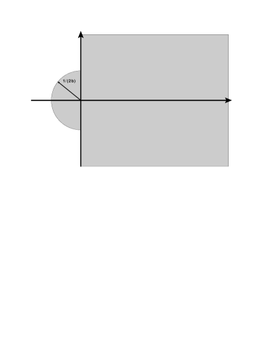
Figure 2: Domain $D$

By the equality (6.14), $\chi$ can be also analytically continued to the domain $D$, which is denoted by $\bar{\chi}$. Let $\epsilon>0$. Then

$$\chi(z)=\sum_{n=0}^{\infty}\left(\!\frac{(-1)^{n}}{n!}\int_{0}^{\infty}\lambda^{n}{\rm e}^{-\epsilon\lambda}\!{\rm d}E(\lambda)\!\right)(z-\epsilon)^{n}$$ (6.16)

for $0<\epsilon-z$, where $\!{\rm d}E(\lambda)$ denotes the spectral resolution of the self-adjoint operator ${\rm A}_{\xi}^{2}$ with respect to $\varphi_{\rm g}^{t}$. Since we have

$$\frac{1}{\sqrt{1+2zb}}\bar{\rho}\circ\theta(z)=\sum_{n=0}^{\infty}a_{n}(z-\epsilon)^{n}$$ (6.17)

for $z\in{{\mathbb{C}}}$ such that $|z-\epsilon|<\sqrt{\frac{1}{(2b)^{2}}+\epsilon^{2}}$. Comparing both expansions (6.16) and (6.17) we see that $a_{n}=\frac{(-1)^{n}}{n!}\int_{0}^{\infty}\lambda^{n}{\rm e}^{-\epsilon\lambda}\!{\rm d}E(\lambda)$ and by (6.17) we have

$$\frac{1}{\sqrt{1+2zb}}\bar{\rho}\circ\theta(z)=\sum_{n=0}^{\infty}\left(\!\frac{(-1)^{n}}{n!}\int_{0}^{\infty}\lambda^{n}{\rm e}^{-\epsilon\lambda}\!{\rm d}E(\lambda)\!\right)(z-\epsilon)^{n}.$$ (6.18)

In particular it follows that for $-\delta<0$ with $\epsilon+\delta<\sqrt{\frac{1}{(2b)^{2}}+\epsilon^{2}}$,

$$\bar{\chi}(\delta)=\sum_{n=0}^{\infty}\left(\!\frac{1}{n!}\int_{0}^{\infty}\lambda^{n}{\rm e}^{-\epsilon\lambda}\!{\rm d}E(\lambda)\!\right)(\delta+\epsilon)^{n}<\infty.$$

Thus

$$\sum_{n=0}^{\infty}\left(\!\frac{1}{n!}\int_{0}^{N}\lambda^{n}{\rm e}^{-\epsilon\lambda}\!{\rm d}E(\lambda)\!\right)(\delta+\epsilon)^{n}=\int_{0}^{N}{\rm e}^{\delta\lambda}\!{\rm d}E(\lambda)$$

and take $N\to\infty$ on both sides we have $\bar{\chi}(\delta)=\int_{0}^{\infty}{\rm e}^{\delta\lambda}\!{\rm d}E(\lambda)<\infty$. Since $\epsilon>0$ is arbitrary, then it follows that $(\varphi_{\rm g}^{t},{\rm e}^{z{\rm A}_{\xi}^{2}}\varphi_{\rm g}^{t})<\infty$ for $\beta>(2b)^{-1}$. $\Box$

Theorem 6.8

(Gaussian domination of the ground state) Let $\beta<(2{\rm q_{\rm E}}({\rm j}_{0}\xi))^{-1}$. Then $\varphi_{\rm g}\in{\rm D}({\rm e}^{\beta{\rm A}_{\xi}^{2}/4})$ follows.

Proof:  By Lemma 6.7 we have the uniform bound $\|{\rm e}^{\beta{\rm A}_{\xi}^{2}}\varphi_{\rm g}^{t}\|^{2}\leq\frac{1}{\sqrt{1-2\beta{\rm q_{\rm E}}({\rm j}_{0}\xi)^{2}}}$ in $t$. Thus there exists a subsequence $t^{\prime}$ such that $\|{\rm e}^{\beta{\rm A}_{\xi}^{2}/4}\varphi_{\rm g}^{t^{\prime}}\|^{2}$ converges to some $c$ as $t^{\prime}\to\infty$. We reset $t^{\prime}$ as $t$. We claim that $\{{\rm e}^{\beta{\rm A}_{\xi}^{2}/4}\varphi_{\rm g}^{t}\}_{t}$ is a Cauchy sequence. Directly we have $\|{\rm e}^{\beta{\rm A}_{\xi}^{2}/4}\varphi_{\rm g}^{t}-{\rm e}^{\beta{\rm A}_{\xi}^{2}/4}\varphi_{\rm g}^{s}\|^{2}=\|{\rm e}^{\beta{\rm A}_{\xi}^{2}/4}\varphi_{\rm g}^{t}\|^{2}+\|{\rm e}^{\beta{\rm A}_{\xi}^{2}/4}\varphi_{\rm g}^{s}\|^{2}-2(\varphi_{\rm g}^{s},{\rm e}^{\beta{\rm A}_{\xi}^{2}/2}\varphi_{\rm g}^{t})$. Note that $\varphi_{\rm g}^{t}$ strongly converges to $\varphi_{\rm g}$ as $t\to\infty$. Since the uniform bound of $\|{\rm e}^{\beta{\rm A}_{\xi}^{2}}\varphi_{\rm g}^{t}\|^{2}$ implies that

$$(\varphi_{\rm g}^{s},{\rm e}^{\beta{\rm A}_{\xi}^{2}/2}\varphi_{\rm g}^{t})=(\varphi_{\rm g}^{s}-\varphi_{\rm g}^{t},{\rm e}^{\beta{\rm A}_{\xi}^{2}/2}\varphi_{\rm g}^{t})+\|{\rm e}^{\beta{\rm A}_{\xi}^{2}/4}\varphi_{\rm g}^{t}\|^{2}\to c$$

as $t,s\to\infty$, we obtain that $\lim_{t,s\to\infty}\|{\rm e}^{\beta{\rm A}_{\xi}^{2}/4}\varphi_{\rm g}^{t}-{\rm e}^{\beta{\rm A}_{\xi}^{2}/4}\varphi_{\rm g}^{s}\|=0$ and ${\rm e}^{\beta{\rm A}_{\xi}^{2}/4}\varphi_{\rm g}^{t}$, $t>0$, is a convergent sequence. Hence the closedness of ${\rm e}^{\beta{\rm A}_{\xi}^{2}/4}$ yields the desired results. $\Box$

7 Measures associated with the ground state

Similar to Section 6 in this section let ${\rm H}={\rm H}_{\rm qf}$ or ${\rm H}_{\rm K}$, and we suppose that ${\rm H}$ has a ground state $\varphi_{\rm g}$.

7.1 Outline

We set $\mathscr{X}=\Omega_{\rm P}\times\Omega_{\nu}$ and ${\rm W}^{x}={\rm P}^{x}\otimes\nu$ in what follows. Let $X_{t}=B_{T_{t}}$ for $t\geq 0$ and $X_{-t}=B_{-T_{t}}$ for $-t<0$. Thus $t\mapsto X_{t}(\omega_{1},\omega_{2})=B_{T_{t}(\omega_{2})}(\omega_{1})$ for $(\omega_{1},\omega_{2})\in\mathscr{X}$ is a cádlág path, i.e., paths are right continuous and the left limits exist. Let ${\cal F}_{[-s,s]}=\sigma(X_{r};r\in[-s,s])$. Then

$$\mathscr{G}_{t}=\bigcup_{0\leq s\leq t}{\cal F}_{[-s,s]},\quad\displaystyle\mathscr{G}=\bigcup_{0\leq s}{\cal F}_{[-s,s]}$$ (7.1)

are finitely additive families of sets. We define the correction of probability spaces by

$$(\mathscr{X},\sigma(\mathscr{G}),\mu_{t}),\quad t>0,$$ (7.2)

where $\mu_{t}$ is given by (6.6). We show in this section that there exists a probability measure $\mu_{\infty}$ on $(\mathscr{X},\sigma(\mathscr{G}))$ such that $\mu_{t}\to\mu_{\infty}$ as $t\to\infty$ in the local weak sense.

The outline of the idea to show the convergence is as follows. First by using $\varphi_{\rm g}^{t}$ we define the family of finitely additive set functions $\rho_{t}$ on $(\mathscr{X},\mathscr{G}_{t})$, $t>0$, and we denote the extension to the probability measure on $(\mathscr{X},\sigma(\mathscr{G}_{t}))$ by $\bar{\rho}_{t}$. Thus we define the probability space

$$(\mathscr{X},\sigma(\mathscr{G}_{t})),\bar{\rho}_{t}).$$ (7.3)

We show in Lemma 7.5 by using functional integrations that

$$\bar{\rho}_{t}(A)=\rho_{t}(A)=\mu_{t}(A)$$ (7.4)

for $A\in\mathscr{G}_{s}$ for all $s\leq t$. Next by using the ground state $\varphi_{\rm g}$ we define a finitely additive set function $\mu$ on $(\mathscr{X},\mathscr{G})$ and denote the extension to the probability measure on $(\mathscr{X},\sigma(\mathscr{G}))$ by $\mu_{\infty}$. Thus we define the probability space

$$(\mathscr{X},\sigma(\mathscr{G})),\mu_{\infty}).$$ (7.5)

By applying the fact that $\varphi_{\rm g}^{t}$ strongly converges to $\varphi_{\rm g}$ as $t\to\infty$, we prove that

$$\rho_{t}(A)\to\mu(A),\quad t\to\infty,$$ (7.6)

for $A\in\mathscr{G}$ in Lemma 7.6, which, together with (7.4), implies that

$$\mu_{t}(A)\to\mu_{\infty}(A),\quad A\in\mathscr{G}$$ (7.7)

and $\mu_{t}$ converges to the measure $\mu_{\infty}$ in the sense of local weak. By the construction of $\mu_{\infty}$ we can show an explicit form of $\mu_{\infty}(A)$ for $A\in\mathscr{G}$. See Figure 3.

$$\mu_{t}\stackrel{{\scriptstyle\rm Lemma\ref{equality}}}{{=}}\rho_{t}\subset\bar{\rho}_{t}\xrightarrow{\rm Lemma\ref{doko}}\mu\subset\mu_{\infty}$$

Figure 3: Local weak convergence of $\mu_{t}$ to $\mu_{\infty}$

7.2 Local weak convergences

Let us define

$${\rm J}_{[-t,t]}={\rm J}_{-t}^{\ast}{\rm e}^{-\int_{-t}^{t}V(X_{s}){\rm d}s}{\rm e}^{-i\alpha{\rm A}_{\rm E}({\rm I}[-t,t])}{\rm J}_{t}.$$ (7.8)

Note that for a.s. $(\omega_{1},\omega_{2})\in\mathscr{X}$, ${\rm J}_{[-t,t]}:L^{2}({\mathscr{Q}})\to L^{2}({\mathscr{Q}})$ is a bounded linear operator. Define an additive set function $\mu:\mathscr{G}\to{\mathbb{R}}$ by

$$\mu(A)={\rm e}^{2Et}\int_{{\mathbb{R}}^{d}}\!{\rm d}x\mathbb{E}_{\rm W}^{x}\!\left[\!{\mathchoice{\rm 1\mskip-4.0mul}{\rm 1\mskip-4.0mul}{\rm 1\mskip-4.5mul}{\rm 1\mskip-5.0mul}}_{A}(\varphi_{\rm g}(X_{-t}),{\rm J}_{[-t,t]}\varphi_{\rm g}(X_{t}))\!\right],\quad A\in{\cal F}_{[-t,t]}.$$ (7.9)

Lemma 7.1

It follows that $\mu(A)\geq 0$ for $A\in{\cal F}_{[-t,t]}$.

Proof:  We note that ${\rm e}^{i\frac{\pi}{2}{\rm N}}\varphi_{\rm g}>0$ and ${\rm e}^{i\frac{\pi}{2}{\rm N}}{\rm J}_{[-t,t]}{\rm e}^{-i\frac{\pi}{2}{\rm N}}$ is positivity improving by Corollary 6.2. Then

$$\mu(A)={\rm e}^{2Et}\int_{{\mathbb{R}}^{d}}\!{\rm d}x\mathbb{E}_{\rm W}^{x}\!\left[\!{\mathchoice{\rm 1\mskip-4.0mul}{\rm 1\mskip-4.0mul}{\rm 1\mskip-4.5mul}{\rm 1\mskip-5.0mul}}_{A}({\rm e}^{i\frac{\pi}{2}{\rm N}}\varphi_{\rm g}(X_{-t}),{\rm e}^{i\frac{\pi}{2}{\rm N}}{\rm J}_{[-t,t]}{\rm e}^{-i\frac{\pi}{2}{\rm N}}{\rm e}^{i\frac{\pi}{2}{\rm N}}\varphi_{\rm g}(X_{t}))\!\right]\geq 0,$$

the lemma follows. $\Box$

Lemma 7.2

The set function $\mu$ is well defined, i.e., for $A\in{\cal F}_{[-t,t]}\subset{\cal F}_{[-s,s]}$

$$\mu(A) ={\rm e}^{2Et}\int_{{\mathbb{R}}^{d}}\!{\rm d}x\mathbb{E}_{\rm W}^{x}\!\left[\!{\mathchoice{\rm 1\mskip-4.0mul}{\rm 1\mskip-4.0mul}{\rm 1\mskip-4.5mul}{\rm 1\mskip-5.0mul}}_{A}(\varphi_{\rm g}(X_{-t}),{\rm J}_{[-t,t]}\varphi_{\rm g}(X_{t}))\!\right]$$

$$={\rm e}^{2Es}\int_{{\mathbb{R}}^{d}}\!{\rm d}x\mathbb{E}_{\rm W}^{x}\!\left[\!{\mathchoice{\rm 1\mskip-4.0mul}{\rm 1\mskip-4.0mul}{\rm 1\mskip-4.5mul}{\rm 1\mskip-5.0mul}}_{A}(\varphi_{\rm g}(X_{-s}),{\rm J}_{[-s,s]}\varphi_{\rm g}(X_{s}))\!\right]$$

Proof:  Let $\mu_{(t)}=\mu\lceil_{{\cal F}_{[-t,t]}}$. Then $\mu_{(t)}$ is a probability measure on $(\mathscr{X},{\cal F}_{[-t,t]})$. Let $-s<-t=t_{0}<t_{1}<\cdots<t_{n}=t<s$. Then by Corollary 3.18 the finite dimensional distribution is given by

$$\mu_{(t)}^{t_{0},...,t_{n}}(A_{0}\times\cdots\times A_{n})=\mu(X_{t_{0}}\in A_{0},\cdots,X_{t_{n}}\in A_{n})$$

$$={\rm e}^{2Et}\int_{{\mathbb{R}}^{d}}\!{\rm d}x\mathbb{E}_{\rm W}^{x}\!\left[\!\left(\!\prod_{j=0}^{n}{\mathchoice{\rm 1\mskip-4.0mul}{\rm 1\mskip-4.0mul}{\rm 1\mskip-4.5mul}{\rm 1\mskip-5.0mul}}_{A_{j}}(X_{t_{j}})\!\right)(\varphi_{\rm g}(X_{-t}),{\rm J}_{[-t,t]}\varphi_{\rm g}(X_{t}))\!\right]$$

$$=(\varphi_{\rm g},{\mathchoice{\rm 1\mskip-4.0mul}{\rm 1\mskip-4.0mul}{\rm 1\mskip-4.5mul}{\rm 1\mskip-5.0mul}}_{A_{0}}{\rm e}^{-(t_{1}-t_{0})({\rm H}-E)}\cdots{\rm e}^{-(t_{n}-t_{n-1})({\rm H}-E)}{\mathchoice{\rm 1\mskip-4.0mul}{\rm 1\mskip-4.0mul}{\rm 1\mskip-4.5mul}{\rm 1\mskip-5.0mul}}_{A_{n}}\varphi_{\rm g}).$$

By ${\rm e}^{-(t_{0}+s)({\rm H}-E)}\varphi_{\rm g}=\varphi_{\rm g}$ we have

$$=(\varphi_{\rm g},{\rm e}^{-(t_{0}+s)({\rm H}-E)}{\mathchoice{\rm 1\mskip-4.0mul}{\rm 1\mskip-4.0mul}{\rm 1\mskip-4.5mul}{\rm 1\mskip-5.0mul}}_{A_{0}}{\rm e}^{-(t_{1}-t_{0}){\rm H}}\cdots{\rm e}^{-(t_{n}-t_{n-1}){\rm H}}{\mathchoice{\rm 1\mskip-4.0mul}{\rm 1\mskip-4.0mul}{\rm 1\mskip-4.5mul}{\rm 1\mskip-5.0mul}}_{A_{n}}{\rm e}^{-(s-t_{n})({\rm H}-E)}\varphi_{\rm g})$$

$$={\rm e}^{2Es}\int_{{\mathbb{R}}^{d}}\!{\rm d}x\mathbb{E}_{\rm W}^{x}\!\left[\!\left(\!\prod_{j=0}^{n}{\mathchoice{\rm 1\mskip-4.0mul}{\rm 1\mskip-4.0mul}{\rm 1\mskip-4.5mul}{\rm 1\mskip-5.0mul}}_{A_{j}}(X_{t_{j}})\!\right)(\varphi_{\rm g}(X_{-s}),{\rm J}_{[-s,s]}\varphi_{\rm g}(X_{s}))\!\right]$$

$$=\mu_{(s)}^{t_{0},...,t_{n}}(A_{0}\times\cdots\times A_{n}).$$

It can be also seen that the finite dimensional distributions $\mu_{(t)}^{\Lambda}$, $\Lambda\subset[-t,t],\#\Lambda<\infty$, satisfy the consistency condition, i.e.,

$$\mu_{(t)}^{t_{0},...,t_{n}}(A_{0}\times\cdots\times A_{n})=\mu_{(t)}^{t_{0},...,t_{n},t_{n+1},...,t_{n+l}}(A_{0}\times\cdots\times A_{n}\times\prod^{l}{{\mathbb{R}}^{d}}).$$

By the Kolmogorov extension theorem there exists a unique probability space $({\cal Y},\mathscr{B}_{\rm q},{\rm q})$ and a stochastic process $(Y_{s})_{s\in[-t,t]}$ up to isomorphisms (e.g., [Sim05, Theorem 2.1]) such that $\mathscr{B}_{\rm q}$ is the minimal $\sigma$-field, $\mathscr{B}_{\rm q}=\sigma(Y_{s},s\in[-t,t])$, and $\mu^{t_{0},...,t_{n}}_{(t)}(A_{0}\times\cdots\times A_{n})={\rm q}(Y_{t_{0}}\in A_{0},\cdots,Y_{t_{n}}\in A_{n})$. By the uniqueness, $({\cal Y},\mathscr{B}_{\rm q},{\rm q})$ and $({\mathscr{X}},{\cal F}_{[-t,t]},\mu_{(t)})$ are isomorphic, and also is $({\cal Y},\mathscr{B}_{\rm q},{\rm q})$ and $({\mathscr{X}},{\cal F}_{[-t,t]},\mu_{(s)}\lceil_{{\cal F}_{[-t,t]}})$. Hence ${\rm q}(A)=\mu_{(s)}(A)=\mu_{(t)}(A)$ for $A\in{\cal F}_{[-t,t]}$ follows. $\Box$

Clearly $\mu$ is a completely additive set function on $(\mathscr{X},\mathscr{G})$. There exists a unique probability measure $\mu_{\infty}$ on $(\mathscr{X},\sigma(\mathscr{G}))$ such that $\mu_{\infty}(A)=\mu(A)$ for $A\in\mathscr{G}$ by the Hopf theorem.

Theorem 7.3

(Local weak convergence and uniqueness) The probability measures $\mu_{t}$ converges to $\mu_{\infty}$ in the local weak sense, i.e., $\mu_{t}(A)\to\mu_{\infty}(A)$ as $t\to\infty$ for each $A\in\mathscr{G}$, and $\mu_{\infty}$ is independent of $\phi$.

Before giving a proof of Theorem 7.3 we need several lemmas. We define an additive set function $\rho_{t}:\mathscr{G}_{t}\to{\mathbb{R}}$ by

$$\rho_{t}(A)={\rm e}^{2Es}\int_{{\mathbb{R}}^{d}}\!\!\!\!{\rm d}x\mathbb{E}_{\rm W}^{x}\!\left[\!{\mathchoice{\rm 1\mskip-4.0mul}{\rm 1\mskip-4.0mul}{\rm 1\mskip-4.5mul}{\rm 1\mskip-5.0mul}}_{A}\left(\!\frac{\phi_{t-s}(X_{0})}{\|\phi_{t}\|},{\rm J}_{[-s,s]}\frac{\phi_{t-s}(X_{s})}{\|\phi_{t}\|}\!\right)\!\right]$$ (7.10)

for $A\in{\cal F}_{[-s,s]}$ with $s\leq t$.

Lemma 7.4

The set function $\rho_{t}$ satisfies $\rho_{t}(A)\geq 0$ and is well defined, i.e.,

$$\rho_{t}(A) ={\rm e}^{2Er}\int_{{\mathbb{R}}^{d}}\!\!\!\!{\rm d}x\mathbb{E}_{\rm W}^{x}\!\left[\!{\mathchoice{\rm 1\mskip-4.0mul}{\rm 1\mskip-4.0mul}{\rm 1\mskip-4.5mul}{\rm 1\mskip-5.0mul}}_{A}\left(\!\frac{\phi_{t-r}(X_{-r})}{\|\phi_{t}\|},{\rm J}_{[-r,r]}\frac{\phi_{t-r}(X_{r})}{\|\phi_{t}\|}\!\right)\!\right]$$

$$={\rm e}^{2Es}\int_{{\mathbb{R}}^{d}}\!\!\!\!{\rm d}x\mathbb{E}_{\rm W}^{x}\!\left[\!{\mathchoice{\rm 1\mskip-4.0mul}{\rm 1\mskip-4.0mul}{\rm 1\mskip-4.5mul}{\rm 1\mskip-5.0mul}}_{A}\left(\!\frac{\phi_{t-s}(X_{-s})}{\|\phi_{t}\|},{\rm J}_{[-s,s]}\frac{\phi_{t-s}(X_{s})}{\|\phi_{t}\|}\!\right)\!\right]$$ (7.11)

for all $r\leq s\leq t$.

Proof:  $\rho_{t}(A)\geq 0$ follows in a similar way to Lemma 7.1. The proof of the second statement is similar to that of Lemma 7.2. The left-hand side of (7.11) is denoted by $\rho_{(r)}(A)$ and the right-hand side by $\rho_{(s)}(A)$. The finite dimensional distribution of $\rho_{(r)}$ is given by

$$\rho_{(r)}^{t_{0},...,t_{n}}(A_{0}\times\cdots\times A_{n})=\rho_{(r)}(X_{t_{0}}\in A_{0},...,X_{t_{n}}\in A_{n})$$

$$=\frac{{\rm e}^{2Er}}{\|\phi_{t}\|^{2}}\int_{{\mathbb{R}}^{d}}\!{\rm d}x\mathbb{E}_{\rm W}^{x}\!\left[\!\left(\!\prod_{j=0}^{n}{\mathchoice{\rm 1\mskip-4.0mul}{\rm 1\mskip-4.0mul}{\rm 1\mskip-4.5mul}{\rm 1\mskip-5.0mul}}_{A_{j}}(X_{t_{j}})\!\right)({\phi_{t-r}(X_{-r})},{\rm J}_{[-r,r]}{\phi_{t-r}(X_{r})}\!\right].$$

By Corollary 3.18 the right-hand side above can be represented as

$$=\frac{1}{\|\phi_{t}\|^{2}}{\left(\!{\phi_{t-r}},{\rm e}^{-(t_{0}+r)({\rm H}-E)}{\mathchoice{\rm 1\mskip-4.0mul}{\rm 1\mskip-4.0mul}{\rm 1\mskip-4.5mul}{\rm 1\mskip-5.0mul}}_{A_{0}}{\rm e}^{-(t_{1}-t_{0})({\rm H}-E)}\cdots{\rm e}^{-(t_{n}-t_{n-1})({\rm H}-E)}{\mathchoice{\rm 1\mskip-4.0mul}{\rm 1\mskip-4.0mul}{\rm 1\mskip-4.5mul}{\rm 1\mskip-5.0mul}}_{A_{n}}{\rm e}^{-(r-t_{n})({\rm H}-E)}{\phi_{t-r}}\!\right)}$$

$$=\frac{1}{\|\phi_{t}\|^{2}}\left(\!{\phi\otimes{\mathchoice{\rm 1\mskip-4.0mul}{\rm 1\mskip-4.0mul}{\rm 1\mskip-4.5mul}{\rm 1\mskip-5.0mul}}},{\rm e}^{-(t+t_{0})({\rm H}-E)}{\mathchoice{\rm 1\mskip-4.0mul}{\rm 1\mskip-4.0mul}{\rm 1\mskip-4.5mul}{\rm 1\mskip-5.0mul}}_{A_{0}}{\rm e}^{-(t_{1}-t_{0})({\rm H}-E)}\cdots{\rm e}^{-(t_{n}-t_{n-1})({\rm H}-E)}{\mathchoice{\rm 1\mskip-4.0mul}{\rm 1\mskip-4.0mul}{\rm 1\mskip-4.5mul}{\rm 1\mskip-5.0mul}}_{A_{n}}{\rm e}^{-(t-t_{n})({\rm H}-E)}{\phi\otimes{\mathchoice{\rm 1\mskip-4.0mul}{\rm 1\mskip-4.0mul}{\rm 1\mskip-4.5mul}{\rm 1\mskip-5.0mul}}}\!\right)$$

$$=\frac{1}{{\|\phi_{t}\|^{2}}}\left(\!{\phi_{t-s}},{\rm e}^{-(t_{0}+s)({\rm H}-E)}{\mathchoice{\rm 1\mskip-4.0mul}{\rm 1\mskip-4.0mul}{\rm 1\mskip-4.5mul}{\rm 1\mskip-5.0mul}}_{A_{0}}{\rm e}^{-(t_{1}-t_{0})({\rm H}-E)}\cdots{\rm e}^{-(t_{n}-t_{n-1})({\rm H}-E)}{\mathchoice{\rm 1\mskip-4.0mul}{\rm 1\mskip-4.0mul}{\rm 1\mskip-4.5mul}{\rm 1\mskip-5.0mul}}_{A_{n}}{\rm e}^{-(s-t_{n})({\rm H}-E)}{\phi_{t-s}}\!\right)$$

$$=\frac{{\rm e}^{2Es}}{\|\phi_{t}\|^{2}}\int_{{\mathbb{R}}^{d}}\!{\rm d}x\mathbb{E}_{\rm W}^{x}\!\left[\!\left(\!\prod_{j=0}^{n}{\mathchoice{\rm 1\mskip-4.0mul}{\rm 1\mskip-4.0mul}{\rm 1\mskip-4.5mul}{\rm 1\mskip-5.0mul}}_{A_{j}}(X_{t_{j}})\!\right)({\phi_{t-s}(X_{-s})},{\rm J}_{[-s,s]}{\phi_{t-s}(X_{s})})\!\right]$$

$$=\rho_{(s)}^{t_{0},...,t_{n}}(A_{0}\times\cdots\times A_{n}).$$

Note that $\rho_{(r)}^{\Lambda}$ and $\rho_{(s)}^{\Lambda}$, $\Lambda\subset[-t,t]$, $\#\Lambda<\infty$, satisfy the consistency condition. Note that $\rho_{(r)}\lceil_{{\cal F}_{[-r,r]}}$ and $\rho_{(s)}\lceil_{{\cal F}_{[-r,r]}}$ are probability measures on $(\mathscr{X},{\cal F}_{[-r,r]})$. By the Kolmogorov extension theorem we see that $\rho_{(r)}(A)=\rho_{(s)}(A)$ for $A\in{\cal F}_{[-r,r]}\subset{\cal F}_{[-s,s]}$. Then the lemma follows. $\Box$

By the Hopf theorem there exists a probability measure $\bar{\rho}_{t}$ on $(\mathscr{X},\sigma(\mathscr{G}_{r}))$ such that $\rho_{t}=\bar{\rho}_{t}\lceil_{\mathscr{G}_{t}}$.

Lemma 7.5

Let $s\leq t$ and $A\in\mathscr{G}_{s}$. Then $\bar{\rho}_{t}(A)=\mu_{t}(A)$.

Proof:  For $\Lambda=\{t_{0},t_{1},\cdots,t_{n}\}\subset[-s,s]$ and $\displaystyle A_{0}\times\cdots\times A_{n}\in\times_{j=0}^{n}\mathscr{B}({{\mathbb{R}}^{d}})$, we define

$$\rho_{t}^{\Lambda}(A_{0}\times\cdots\times A_{n}) =\rho_{t}(X_{t_{0}}\in A_{0},...,X_{t_{n}}\in A_{n})$$

$$=\frac{{\rm e}^{2Es}}{{\|\phi_{t}\|}^{2}}\int_{{\mathbb{R}}^{d}}\!\!\!\!{\rm d}x\mathbb{E}_{\rm W}^{x}\!\left[\!\left(\!\prod_{j=0}^{n}{\mathchoice{\rm 1\mskip-4.0mul}{\rm 1\mskip-4.0mul}{\rm 1\mskip-4.5mul}{\rm 1\mskip-5.0mul}}_{A_{j}}(X_{{t_{j}}})\!\right)\left(\!{\phi_{t-s}(X_{-s})},{\rm J}_{[-s,s]}{\phi_{t-s}(X_{s})}\!\right)\!\right]$$

and

$$\mu_{t}^{\Lambda}(A_{0}\times\cdots\times A_{n})=\mu_{t}(X_{t_{0}}\in A_{0},...,X_{t_{n}}\in A_{n})=\frac{1}{Z_{t}}\int_{{\mathbb{R}}^{d}}\!\!\!\!{\rm d}x\mathbb{E}_{\rm W}^{x}\!\left[\!\left(\!\prod_{j=0}^{n}{\mathchoice{\rm 1\mskip-4.0mul}{\rm 1\mskip-4.0mul}{\rm 1\mskip-4.5mul}{\rm 1\mskip-5.0mul}}_{A_{j}}(X_{{t_{j}}})\!\right)\mathscr{L}_{t}\!\right].$$

Both $\rho_{t}^{\Lambda}$ and $\mu_{t}^{\Lambda}$ are probability measures on $(({{\mathbb{R}}^{d}})^{\Lambda},\mathscr{B}({{\mathbb{R}}^{d}})^{\Lambda})$. We have

$$\mu_{t}^{\Lambda}(A_{0}\times\cdots\times A_{n}) =\frac{(\phi\otimes{\mathchoice{\rm 1\mskip-4.0mul}{\rm 1\mskip-4.0mul}{\rm 1\mskip-4.5mul}{\rm 1\mskip-5.0mul}},{\rm e}^{-(t_{0}+t){\rm H}}{\mathchoice{\rm 1\mskip-4.0mul}{\rm 1\mskip-4.0mul}{\rm 1\mskip-4.5mul}{\rm 1\mskip-5.0mul}}_{A_{0}}{\rm e}^{-(t_{1}-t_{0}){\rm H}}{\mathchoice{\rm 1\mskip-4.0mul}{\rm 1\mskip-4.0mul}{\rm 1\mskip-4.5mul}{\rm 1\mskip-5.0mul}}_{A_{1}}\cdots{\mathchoice{\rm 1\mskip-4.0mul}{\rm 1\mskip-4.0mul}{\rm 1\mskip-4.5mul}{\rm 1\mskip-5.0mul}}_{A_{n}}{\rm e}^{-(t-t_{n}){\rm H}}\phi\otimes{\mathchoice{\rm 1\mskip-4.0mul}{\rm 1\mskip-4.0mul}{\rm 1\mskip-4.5mul}{\rm 1\mskip-5.0mul}})}{\|\phi_{t}\|^{2}}$$

$$=\frac{{\rm e}^{2Es}(\phi_{t-s},{\rm e}^{-(t_{0}+s){\rm H}}{\mathchoice{\rm 1\mskip-4.0mul}{\rm 1\mskip-4.0mul}{\rm 1\mskip-4.5mul}{\rm 1\mskip-5.0mul}}_{A_{0}}{\rm e}^{-(t_{1}-t_{0}){\rm H}}{\mathchoice{\rm 1\mskip-4.0mul}{\rm 1\mskip-4.0mul}{\rm 1\mskip-4.5mul}{\rm 1\mskip-5.0mul}}_{A_{1}}\cdots{\mathchoice{\rm 1\mskip-4.0mul}{\rm 1\mskip-4.0mul}{\rm 1\mskip-4.5mul}{\rm 1\mskip-5.0mul}}_{A_{n}}{\rm e}^{-(s-t_{n}){\rm H}}\phi_{t-s})}{\|\phi_{t}\|^{2}}$$

by the definition of $\phi_{t-s}$. The right-hand side above can be expressed as

$$={\rm e}^{2Es}\int_{{\mathbb{R}}^{d}}\!\!\!\!{\rm d}x\mathbb{E}_{\rm W}^{x}\!\left[\!\left(\!\prod_{j=0}^{n}{\mathchoice{\rm 1\mskip-4.0mul}{\rm 1\mskip-4.0mul}{\rm 1\mskip-4.5mul}{\rm 1\mskip-5.0mul}}_{A_{j}}(X_{{t_{j}}})\!\right)\left(\!\frac{\phi_{t-s}(X_{0})}{\|\phi_{t}\|},{\rm J}_{[-s,s]}\frac{\phi_{t-s}(X_{s})}{\|\phi_{t}\|}\!\right)\!\right].$$

Then $\rho_{t}^{\Lambda}(A_{0}\times\cdots\times A_{n})=\mu_{t}^{\Lambda}(A_{0}\times\cdots\times A_{n})$ follows. The probability measures $\mu_{t}^{\Lambda}$ and $\rho_{t}^{\Lambda}$ satisfy the consistency condition. Then by the Kolmogorov extension theorem there exists a unique probability space $({\cal Y},\mathscr{B}_{\rm q},{\rm q})$ and stochastic process $Y_{s}$ such that $\mathscr{B}_{\rm q}=\sigma(Y_{s},s\in[-t,t])$ and ${\rm q}(Y_{t_{0}}\in A_{0},\cdots,Y_{t_{n}}\in A_{n})=\mu_{t}^{t_{0},...,t_{n}}(A_{0}\times\cdots\times A_{n})=\rho_{t}^{t_{0},...,t_{n}}(A_{0}\times\cdots\times A_{n})$. On the other hand it holds that $\mu_{t}^{t_{0},...,t_{n}}(A_{0}\times\cdots\times A_{n})=\rho_{t}^{t_{0},...,t_{n}}(A_{0}\times\cdots\times A_{n})=\bar{\rho}_{t}(A_{0}\times\cdots\times A_{n})=\mu_{t}\lceil_{{\mathscr{G}}_{t}}(A_{0}\times\cdots\times A_{n})$. Hence $\bar{\rho}_{t}={\rm q}=\mu_{t}\lceil_{{\mathscr{G}}_{t}}$ follows by the uniqueness of extensions. $\Box$

Lemma 7.6

Let $A\in\mathscr{G}$. Then $\displaystyle\lim_{t\to\infty}\mu_{t}(A)=\mu_{\infty}(A)$.

Proof:  Suppose that $A\in\mathscr{G}_{s}$ with some $s$. By Lemma 7.5 we have

$$\lim_{t\to\infty}\mu_{t}(A)=\lim_{t\to\infty}\bar{\rho}_{t}(A)=\lim_{t\to\infty}{\rm e}^{2Es}\int_{{\mathbb{R}}^{d}}\!\!\!\!{\rm d}x\mathbb{E}_{\rm W}^{x}\!\left[\!{\mathchoice{\rm 1\mskip-4.0mul}{\rm 1\mskip-4.0mul}{\rm 1\mskip-4.5mul}{\rm 1\mskip-5.0mul}}_{A}\left(\!\frac{\phi_{t-s}(X_{-s})}{\|\phi_{t}\|},{\rm J}_{[-s,s]}\frac{\phi_{t-s}(X_{s})}{\|\phi_{t}\|}\!\right)\!\right].$$

Since $\phi_{t}\to\varphi_{\rm g}$ strongly as $t\to\infty$, we have

$$\lim_{t\to\infty}\mu_{t}(A)={\rm e}^{2Es}\int_{{\mathbb{R}}^{d}}\!\!\!\!{\rm d}x\mathbb{E}_{\rm W}^{x}\!\left[\!{\mathchoice{\rm 1\mskip-4.0mul}{\rm 1\mskip-4.0mul}{\rm 1\mskip-4.5mul}{\rm 1\mskip-5.0mul}}_{A}\left(\!\varphi_{\rm g}(X_{-s}),{\rm J}_{[-s,s]}\varphi_{\rm g}(X_{s})\!\right)\!\right]=\mu_{\infty}(A).$$

Then the lemma follows. $\Box$

Now we state the proof of Theorem 7.3.

Proof of Theorem 7.3: By Lemma 7.6 it follows that $\mu_{t}(A)\to\mu_{\infty}(A)$ for $A\in\mathscr{G}$. Next we show that $\mu_{\infty}$ is independence of the choice of $\phi$. Suppose that $\mu_{\infty}^{\prime}$ is a local weak limit of $\mu_{t}^{\prime}$ defined by $\mu_{t}$ with $\phi$ replace by $\phi^{\prime}$ such that $0\leq\phi^{\prime}\in{L^{2}({{\mathbb{R}}^{d}})}$. By the construction of $\mu_{\infty}$, $\mu_{\infty}(A)=\mu_{\infty}^{\prime}(A)$ for $A\in\mathscr{G}$. The uniqueness of Hopf’s extension implies $\mu_{\infty}=\mu_{\infty}^{\prime}$. Thus $\mu_{\infty}$ is independent of the choice of $\phi$. Then the theorem follows. $\Box$

8 Concluding remarks

8.1 Translation invariant models

Let ${\rm H}={\rm H}_{\rm K}$ or ${\rm H}_{\rm qf}$. Suppose that $V=0$. Then we already see that ${\rm e}^{-it{\rm P}}{\rm e}^{-t{\rm H}}{\rm e}^{it{\rm P}}={\rm e}^{-t{\rm H}}$. Then ${\rm H}$ can be decomposable with respect to the spectrum of ${\rm P}$. Thus we have

$${\rm H}=\int_{{\mathbb{R}}^{d}}^{\oplus}{\rm H}(p)dp.$$ (8.1)

Here ${\rm H}(p)$ is defined by

$${\rm H}(p)=\sqrt{L(p)+m^{2}}-m\ \dot{+}\ {\rm H}_{\rm rad}$$ (8.2)

and

$$L(p)=\overline{(p-{{\rm P}_{\rm f}}-\alpha{\rm A}(0))^{2}\lceil_{D({{\rm P}_{\rm f}}^{2})\cap D({\rm H}_{\rm rad})}}.$$ (8.3)

It is established that $(p-{{\rm P}_{\rm f}}-\alpha{\rm A}(0))^{2}$ is essentially self-adjoint on $D({{\rm P}_{\rm f}}^{2})\cap D({\rm H}_{\rm rad})$ in [Hir07, Theorem 2.3]. We can construct the functional integral representation of ${\rm e}^{-t{\rm H}(p)}$ for each $p\in{{\mathbb{R}}^{d}}$ in a similar manner to [Hir07].

Theorem 8.1

Let $F,G\in L^{2}({\mathscr{Q}})$. Then it follows that

$$(F,{\rm e}^{-t{\rm H}(p)}G)=\mathbb{E}_{{\rm P}\!\times\!\nu}^{0,0}\!\left[\!{\rm e}^{-ip\cdot B_{T_{t}}}\left(\!{\rm J}_{0}F(B_{T_{0}}),{\rm e}^{i{{\rm P}_{\rm f}}\cdot B_{T_{t}}}{\rm e}^{-i\alpha{\rm A}_{\rm E}({\rm I}[0,t])}{\rm J}_{t}G(B_{T_{t}})\!\right)\!\right].$$ (8.4)

From this functional integral representation we can show the self-adjointness of ${\rm H}(p)$ in a similar manner to ${\rm H}$.

Corollary 8.2

Suppose Assumptions 2.1 and 2.2. Then for all $p\in{{\mathbb{R}}^{d}}$, ${\rm H}(p)$ is self-adjoint on ${\rm D}(|{{\rm P}_{\rm f}}|)\cap{\rm D}({\rm H}_{\rm rad})$.

Proof:  The proof is similar to that of Theorems 4.5 and 4.7, i.e, it can be show that ${\rm e}^{-t{\rm H}(p)}$ leaves ${\rm D}(|{{\rm P}_{\rm f}}|)\cap{\rm D}({\rm H}_{\rm rad})$ invariant fo r$m>0$, and that by using the inequality $\||p-{{\rm P}_{\rm f}}|\Phi\|^{2}+\|{\rm H}_{\rm rad}\Phi\|\leq C\|({\rm H}(p)+{\mathchoice{\rm 1\mskip-4.0mul}{\rm 1\mskip-4.0mul}{\rm 1\mskip-4.5mul}{\rm 1\mskip-5.0mul}})\Phi\|$ we can show the self-adjointness of ${\rm H}(p)$ for $m\geq 0$. See [HH13b]. $\Box$

8.2 Spin 1/2 and generalizations

Let us assume that the space dimension $d=3$. The SRPF Hamiltonian with spin ${1/2}$ is defined by

$${\rm H}_{\rm SR}=\sqrt{(\sigma\cdot({\rm p}-\alpha{\rm A}))^{2}+m^{2}}-m+V+{\rm H}_{\rm rad}$$ (8.5)

on the Hilbert space $\left(\!{{\mathbb{C}}}^{2}\otimes L^{2}({\mathbb{R}}^{3})\!\right)\otimes L^{2}({\mathscr{Q}})$. Here $\sigma=(\sigma_{1},\sigma_{2},\sigma_{3})$ are the $2\times 2$ Pauli matrices given by

$$\sigma_{1}=\left[\!\!\!\begin{array}[]{cc}0&1\\ 1&0\end{array}\!\!\!\right],\ \ \ \sigma_{2}=\left[\!\!\!\begin{array}[]{cc}0&-i\\ i&0\end{array}\!\!\!\right],\ \ \ \sigma_{3}=\left[\!\!\!\begin{array}[]{cc}1&0\\ 0&-1\end{array}\!\!\!\right].$$ (8.6)

Let $(N_{t})_{t\geq 0}$ be the Poisson process with the unit intensity on a probability space $(\Omega_{\nu},\mathscr{B}_{\nu},\nu)$. We define the stochastic process $\sigma_{t}=\sigma(-1)^{N_{t}}$, $t\geq 0$, where $\sigma\in\{-1,+1\}$. Under some condition we can construct a functional integral representation of ${\rm e}^{-t{\rm H}}$ in terms of stochastic processes $(B_{t})_{t\geq 0}$, $(T_{t})_{t\geq 0}$ and $(\sigma_{t})_{t\geq 0}$. We can identify $\left(\!{{\mathbb{C}}}^{2}\otimes L^{2}({\mathbb{R}}^{3})\!\right)\otimes L^{2}({\mathscr{Q}})$ with $L^{2}({\mathbb{R}}^{3}\times\{\pm 1\};L^{2}({\mathscr{Q}}))$. Under this identification we can construct the Feynman-Kac type formula of $e^{-t{\rm H}}$ with

$${\rm H}_{\rm NR}=\frac{1}{2}(\sigma\cdot({\rm p}-\alpha{\rm A}))^{2}+V+{\rm H}_{\rm rad}$$

in [HL08]. By a minor modification we can also construct the Feynman-Kac type formula for ${\rm H}$ in (8.5).

Theorem 8.3

Let $F,G\in L^{2}({\mathbb{R}}^{3}\times\{\pm 1\};L^{2}({\mathscr{Q}}))$. Then

$$(F,{\rm e}^{-t{\rm H}_{\rm SR}}G)={\rm e}^{T_{t}}\sum_{\sigma=\pm 1}\int_{{\mathbb{R}}^{3}}\!{\rm d}x\mathbb{E}_{{\rm P}\times\mu\times\nu}^{x,0,\sigma}\left[\!{\rm e}^{-\int_{0}^{t}V(B_{T_{s}}){\rm d}s}\left(\!{\rm J}_{0}F(B_{T_{0}},\sigma_{T_{0}}),{\rm e}^{S}{\rm J}_{t}G(B_{T_{t}},\sigma_{T_{t}})\!\right)\!\right],$$ (8.7)

where

$$S= -i\alpha{\rm A}_{\rm E}({\rm I}[0,t])-\frac{\alpha}{2}\int_{0}^{T_{t}}\!\!\!\sigma_{s}{\rm B}_{3}(\lambda(\cdot-B_{s})){\rm d}s$$

$$+\int_{0}^{T_{t}+}\!\!\!\!\!\!\log\left(\!\frac{\alpha}{2}({\rm B}_{1}(\lambda(\cdot-B_{s}))-i\sigma_{s}{\rm B}_{2}(\lambda(\cdot-B_{s}))\!\right)dN_{s}$$

and ${\rm B}(x)=\nabla_{x}\times{\rm A}_{\rm E}(x)$ describes the quantized magnetic field.

We can furthermore consider general Hamiltonians of the form:

$$\Psi\left(\!\frac{1}{2}(\sigma\cdot({\rm p}-\alpha{\rm A}))^{2}\!\right)+V+{\rm H}_{\rm rad},$$ (8.8)

where $\Psi$ denotes a Bernstein function. The standard Pauli-Fierz Hamiltonian is realized by $\Psi(u)=u$, and the SRPF Hamiltonian with spin ${1/2}$ by $\Psi(u)=\sqrt{2u+m^{2}}-m$. (8.8) can be also investigated by path measures, and only the difference from (8.7) is to take the subordinator $({T^{\Psi}}_{t})_{t\geq 0}$ associated with Bernstein function $\Psi$ instead of $(T_{t})_{t\geq 0}$. See Appendix F for relationship between Bernstein functions and subordinatos. We will publish details somewhere in near future.

Remark 8.4

We give comments on both of semigroups (8.4) and (8.7).
(1) The semigroup (8.4) is not positivity improving for $p\not=0$ and positivity improving for $p=0$, since the semigroup includes $e^{-ip\cdot B_{T_{t}}}$.
(2) Let $V$ and ${\hat{\varphi}}$ be rotation invariant. Then in a similar manner to [LHB11, Corollary 7.70] it can be shown that (8.5) has degenerate ground state if it exists. In particular in this case (8.7) can not be positivity improving.

8.3 Gaussian domination and local weak convergence

We can see that ${\rm q_{\rm E}}({\rm I}[-t,t],{\rm j}_{0}\xi)$ in (6.12) converges as $t\to\infty$.

Lemma 8.5

Sequence $\{{\rm q_{\rm E}}({\rm I}[-t,t],{\rm j}_{0}\xi)\}_{t}$ is a Cauchy sequence in $L^{2}(\mathscr{X},{\rm W}^{0})$.

Proof:  Let $s<t$ and we estimate $\mathbb{E}_{\rm W}^{0}[{\rm q_{\rm E}}({\rm I}[s,t],{\rm j}_{0}\xi)^{2}]$. By the definition of ${\rm I}[s,t]$ we have

$$\mathbb{E}_{\rm W}^{0}[{\rm q_{\rm E}}({\rm I}[s,t],{\rm j}_{0}\xi)^{2}]\leq\lim_{n\rightarrow\infty}\mathbb{E}_{\rm W}^{0}\left[\!\left|\sum_{j=1}^{2^{n}}\int_{T_{t_{j-1}}}^{T_{t_{j}}}({\rm j}_{t_{j-1}}\lambda(\cdot-B_{s}),{\rm j}_{0}\xi)\!{\rm d}B_{s}\right|^{2}\!\right].$$

By the independent increments of the Brownian motion we have

$$\leq\lim_{n\rightarrow\infty}\sum_{j=1}^{2^{n}}\mathbb{E}_{\rm W}^{0}\left[\!\int_{T_{t_{j-1}}}^{T_{t_{j}}}\!\!\!(\xi,{\rm e}^{-2t_{j-1}\omega}\xi){\rm d}s\!\right]\!\!\|\lambda\|^{2}\!\!\!=\!\!\!\lim_{n\rightarrow\infty}\sum_{j=1}^{2^{n}}\mathbb{E}_{\rm W}^{0}\left[\!(T_{t_{j}}-T_{t_{j-1}})(\xi,{\rm e}^{-2t_{j-1}\omega}\xi)\!\right]\!\!\|\lambda\|^{2}.$$

Since $T_{t_{j}-t_{j-1}}$ and $T_{t_{j}}-T_{t_{j-1}}$ have the same low, we see that

$$=\left(\!\xi,\lim_{n\rightarrow\infty}\sum_{j=1}^{2^{n}}\mathbb{E}_{\rm W}^{0}\left[\!T_{t_{j}-t_{j-1}}{\rm e}^{-2t_{j-1}\omega}\!\right]\xi\!\right)\|\lambda\|^{2}.$$

Using the distribution of $T_{t}$ we have

$$=\left(\!\xi,\lim_{n\rightarrow\infty}\sum_{j=1}^{2^{n}}\left(\!\int_{0}^{\infty}{\rm d}s\frac{\Delta t_{j}}{\sqrt{2\pi}}\frac{1}{\sqrt{s}}\exp\left(\!-\frac{1}{2}(\frac{(\Delta t_{j})^{2}}{s}+m^{2}s)\!\right){\rm e}^{-2t_{j-1}\omega}\!\right)\xi\!\right)\|\lambda\|^{2},$$

where $\Delta t_{j}=t_{j}-t_{j-1}$. Since $m>0$ we obtain that

$$\leq C\left(\!\xi,\xi\lim_{n\rightarrow\infty}\sum_{j=1}^{2^{n}}\Delta t_{j}{\rm e}^{-2t_{j-1}\omega}\!\right)=C\left(\!\xi,\xi\int_{s}^{t}{\rm e}^{-2r\omega}{\rm d}r\!\right)=C\left(\!\xi,\frac{{\rm e}^{-2s\omega}-{\rm e}^{-2t\omega}}{2\omega}\xi\!\right)$$

with some constant $C$. Then ${\rm q_{\rm E}}({\rm I}[-t,t],{\rm j}_{0}\xi)$ is a Cauchy sequence. $\Box$

By Lemma 8.5 there exists ${\rm q_{\rm E}}({\rm I}(-\infty,\infty),{\rm j}_{0}\xi)$ such that $\displaystyle\lim_{t\rightarrow\infty}{\rm q_{\rm E}}({\rm I}[-t,t],{\rm j}_{0}\xi)={\rm q_{\rm E}}({\rm I}(-\infty,\infty),{\rm j}_{0}\xi)$ in $L^{2}(\mathscr{X},{\rm W}^{0})$.

Remark 8.6

By Theorem 7.3 and Lemma 8.5 we conjecture that

$$(\varphi_{\rm g},{\rm e}^{\beta{\rm A}_{\xi}^{2}}\varphi_{\rm g})=\frac{1}{\sqrt{1-2\beta{\rm q_{\rm E}}({\rm j}_{0}\xi)}}\mathbb{E}_{\mu_{\infty}}\left[\!{\rm e}^{\frac{-\beta\alpha^{2}{\rm q_{\rm E}}({\rm I}[-\infty,\infty],{\rm j}_{0}\xi)^{2}}{(1-2\beta{\rm q_{\rm E}}({\rm j}_{0}\xi))}}\!\right]$$ (8.9)

and $\lim_{\beta\uparrow{\rm q_{\rm E}}({\rm j}_{0}\xi)/2}\|{\rm e}^{\beta{\rm A}_{\xi}^{2}/2}\varphi_{\rm g}\|=\infty$. This type of results are derived for a spin-boson model [HHL12].

Appendix A Brownian motion on ${\mathbb{R}}$

Let $(B_{t})_{t\in{\mathbb{R}}}$ be $d$-dimensional Brownian motion on a probability space $(\Omega_{\rm P},\mathscr{B}_{\rm P},{\rm P}^{x})$. The properties of Brownian motion on the whole real line can be summarized as follows. Let $N_{t}$ be the Gaussian random variable with mean zero and covariance $t$.

• ${\rm P}^{x}(B_{0}=x)=1$;

• the increments $(B_{t_{i}}-B_{t_{i-1}})_{1\leq i\leq n}$ are independent Gaussian random variables for any $0=t_{0}<t_{1}<\cdots<t_{n}$ with $B_{t}-B_{s}\stackrel{{\scriptstyle\rm d}}{{=}}N_{t-s}$, for $t>s$;

• the increments $(B_{-t_{i-1}}-B_{-t_{i}})_{1\leq i\leq n}$ are independent Gaussian random variables for any $0=-t_{0}>-t_{1}>\cdots>-t_{n}$ with $B_{-t}-B_{-s}\stackrel{{\scriptstyle\rm d}}{{=}}N_{s-t}$, for $-t>-s$;

• the function ${\mathbb{R}}\ni t\mapsto B_{t}(\omega)\in{\mathbb{R}}$ is continuous for almost every $\omega$;

• $B_{t}$ and $B_{s}$ for $t>0$ and $s<0$ are independent;

• the joint distribution of $B_{t_{0}},\ldots,B_{t_{n}}$, $-\infty<t_{0}<t_{1}<\cdots<t_{n}<\infty$, with respect to $\!{\rm d}x\otimes\!{\rm dP}^{x}$ is invariant under time shift, i.e.,

  $$\int_{{\mathbb{R}}^{d}}\!{\rm d}x\mathbb{E}_{\rm P}^{x}\left[\prod_{i=0}^{n}f_{i}(B_{t_{i}})\right]=\int_{{\mathbb{R}}^{d}}\!{\rm d}x\mathbb{E}_{\rm P}^{x}\left[\prod_{i=0}^{n}f_{i}(B_{t_{i}+s})\right]$$ (1.1)

  for all $s\in{\mathbb{R}}$.

Appendix B Proof of Proposition 3.4

Proof of Proposition 3.4: We show an outline of a proof. This is a modification of [Hir00b, Theorem 2.7] and [LHB11, Lemma 7.53]. By the Riesz theorem the right-hand side of (3.5) can be expressed as $(F,S_{t}G)$ with some bounded operator $S_{t}$. We can check that $S_{t}$, $t\geq 0$, is symmetric and strongly continuous one-parameter semigroup. Thus there exists a self-adjoint operator $K$ such that $S_{t}={\rm e}^{-tK}$. It is also shown [Hir97, the proof of Lemma 4.8] that

$$\frac{1}{t}((e^{-tK}-{\mathchoice{\rm 1\mskip-4.0mul}{\rm 1\mskip-4.0mul}{\rm 1\mskip-4.5mul}{\rm 1\mskip-5.0mul}})F,G)=\int_{0}^{1}(-{\rm h}_{\rm A}F,e^{-tsK}G){\rm d}s$$ (2.1)

for $F,G\in C_{0}^{\infty}({{\mathbb{R}}^{d}})\otimes L^{2}_{\rm fin}({\mathscr{Q}})$. By the inequality $\|{\rm h}_{\rm A}F\|\leq C(\|p^{2}F\|+\|({\rm N}+{\mathchoice{\rm 1\mskip-4.0mul}{\rm 1\mskip-4.0mul}{\rm 1\mskip-4.5mul}{\rm 1\mskip-5.0mul}})F\|)$ with some positive constant $C$, (2.1) can be extended for $F,G\in D({\rm p}^{2})\cap D({\rm N})$. Thus $K={\rm h}_{{\rm A}}$ on ${\rm D}({\rm p}^{2})\cap C^{\infty}({\rm N})$. We also see that $|(UF,{\rm e}^{-tK}G)|\leq C(U,K,G)\|F\|$ for $F,G\in D(U)$, where $C(U,K,G)$ is a positive constant, $U={\rm p}^{2}$ and $U={\rm N}^{n}$ for any $n\geq 1$. Thus ${\rm e}^{-tK}$ leaves ${\rm D}({\rm p}^{2})\cap C^{\infty}({\rm N})$ invariant. Thus the proposition follows from Proposition 3.3.

Appendix C Relativistic Kato-class

Let $m\geq 0$. Set $h=\sqrt{{\rm p}^{2}+m^{2}}-m$. It is known that $V\geq 0$ is in the relativistic Kato-class if and only if $\displaystyle\lim_{E\to\infty}\sup_{x\in{{\mathbb{R}}^{d}}}|((h-E)^{-1}V)(x)|=0$. See e.g.[HIL13, Proposition 4.5].

Lemma C.1

Let $V>0$ be in the relativistic Kato-class. Then $V$ is infinitesimally small form bounded with respect to $h$, i.e., for arbitrary $\epsilon$ there exists $b_{\epsilon}\geq 0$ such that $\|V^{1/2}f\|\leq\epsilon\|h^{1/2}f\|+b_{\epsilon}\|f\|$ for arbitrary $f\in D(h^{1/2})$. In particular $\mathscr{V}_{\rm Kato}\subset\mathscr{V}_{\rm qf}$.

Proof:  Let $\|\cdot\|_{p,p}$ be bounded operator norm on $L^{p}({{\mathbb{R}}^{d}})$. By duality it is seen that $\|(h+E)^{-1}V\|_{1,1}=\|(h+E)^{-1}V\|_{\infty,\infty}$. By the Stein interpolation theorem we have $\|V^{1/2}(h-E)^{-1}V^{1/2}\|_{2,2}\leq\|(h+E)^{-1}V\|_{1,1}$ and notice that $\|(h+E)^{-1}V\|_{\infty,\infty}=\sup_{x\in{{\mathbb{R}}^{d}}}|((h-E)^{-1}V)(x)|$. Hence $\|V^{1/2}(h-E)^{-1/2}\|^{2}_{2,2}\leq\sup_{x\in{{\mathbb{R}}^{d}}}|((h-E)^{-1}V)(x)|\to 0$ as $E\to\infty$. From $\|V^{1/2}f\|\leq\|V^{1/2}(h-E)^{-1/2}\|_{2,2}\|(h-E)^{1/2}f\|$ it follows that $V$ is form bounded with an infinitesimally small relative bound. $\Box$

Appendix D Integral ${\rm I}[a,b]$

Proposition D.1

Let $\displaystyle{\rm I}^{\prime}_{n}[0,t]=\bigoplus^{d}_{\mu=1}\sum_{j=1}^{2^{n}}\int_{T_{{t_{j-1}}}}^{T_{{t_{j}}}}{\rm j}_{{t_{j}}}\lambda(\cdot-B_{s})\!{\rm d}B_{s}^{\mu}$. Then $\displaystyle{\rm s}\!\!-\!\!\lim_{n\to\infty}{\rm I}_{n}^{\prime}[0,t]={\rm I}[0,t]$ in $L^{2}(\Omega_{\rm P},{\rm P}^{x})\otimes\mathscr{E}$.

Proof:  We have $\|{\rm I}_{n}^{\prime}[0,t]-{\rm I}_{n}[0,t]\|^{2}=d(T_{t}-T_{0})(\lambda,2(1-{\rm e}^{-t\omega/2^{n}})\lambda)\to 0$ as $n\to\infty$. Then the proof is complete. $\Box$

Proposition D.2

For each $w\in\Omega_{\nu}\setminus\mathscr{N}_{\nu}$, ${\rm I}[0,t]={\rm I}[0,s]+{\rm I}[s,t]$ for $0<s<t$ follows in the sense of $L^{2}(\Omega_{\rm P},{\rm P}^{x})\otimes{\mathscr{E}}$, i.e.,

$$\mathbb{E}_{\rm P}^{x}\left[\!\left\|{\rm I}[0,t]-{\rm I}[0,s]-{\rm I}[s,t]\right\|^{2}_{\mathscr{E}}\!\right]=0.$$ (4.1)

Proof:  By a limiting argument we see that

$$\mathbb{E}_{\rm P}^{x}\left[\!\|{\rm I}[0,t]\|^{2}_{\mathscr{E}}\!\right]=dT_{t}\|{\hat{\varphi}}/\sqrt{\omega}\|^{2}$$ (4.2)

for almost surely in $\nu$. We suppose that $s=at/2^{k}$ with some $a,k\in{\mathbb{N}}$. Then by the definition of ${\rm I}_{n}[0,t]$ we have $\displaystyle{\rm I}[0,t]=\lim_{n\rightarrow\infty}\bigoplus^{d}_{\mu=1}\sum_{j=1}^{2^{n+k}}\int_{T_{t_{j-1}}}^{T_{t_{j}}}{\rm j}_{{t_{j-1}}}\lambda(\cdot-B_{s})\!{\rm d}B_{s}^{\mu}$ with ${t_{j}}=\frac{tj}{2^{n+k}}$, and

$$\sum_{j=1}^{2^{n+k}}\int_{T_{t_{j-1}}}^{T_{t_{j}}}{\rm j}_{{t_{j-1}}}\lambda(\cdot-B_{s})\!{\rm d}B_{s}^{\mu}$$

$$=\sum_{j=1}^{2^{n}a}\int_{T_{{\frac{s}{2^{n}a}(j-1)}}}^{T_{{\frac{s}{2^{n}a}j}}}{\rm j}_{{\frac{s}{2^{n}a}(j-1)}}\lambda(\cdot-B_{r})\!{\rm d}B_{r}^{\mu}+\sum_{j=1}^{2^{n}b}\int_{T_{s+{\frac{t-s}{2^{n}b}(j-1)}}}^{T_{s+{\frac{t-s}{2^{n}b}j}}}{\rm j}_{s+{\frac{t-s}{2^{n}b}(j-1)}}\lambda(\cdot-B_{r})\!{\rm d}B_{r}^{\mu},$$

where $b=2^{k}-a$. Hence ${\rm I}[0,t]={\rm I}[0,s]+{\rm I}[s,t]$ follows. Let $0<s<t$. Then there exists $s(\epsilon)>s$ such that $s(\epsilon)=a/2^{k}$ with some $a,k\in{\mathbb{N}}$ and $s(\epsilon)\downarrow s$ as $\epsilon\to 0$. Hence ${\rm I}[0,t]={\rm I}[0,s(\epsilon)]+{\rm I}[s(\epsilon),t]$. Note that ${\rm I}[0,s(\epsilon)]-{\rm I}[0,s]={\rm I}[s,s(\epsilon)]$ and $\mathbb{E}_{{\rm P}}^{x}\left[\!\|{\rm I}[s,s(\epsilon)]\|^{2}\!\right]=(T_{s(\epsilon)}-T_{s})\|{\hat{\varphi}}/\sqrt{\omega}\|^{2}$ by the Itô isometry (4.2). Since $T_{s}=T_{s}(w)$ is right continuous in $s$ for $w\in\Omega_{\nu}\setminus\mathscr{N}_{\nu}$, (4.1) follows. $\Box$

Proposition D.3

Let $a\leq b$ and $c\leq d$, and suppose that $[a,b]\cap[c,d]=[c,b]$. Then for each $w\in\Omega_{\nu}\setminus\mathscr{N}_{\nu}$, $\mathbb{E}_{{\rm P}}^{x}\left[\!({\rm I}[a,b],{\rm I}[c,d])_{\mathscr{E}}\!\right]=d(T_{b}-T_{c})\|{\hat{\varphi}}/\sqrt{\omega}\|^{2}_{L^{2}({{\mathbb{R}}^{d}})}$.

Proof:  Suppose that $[a,b]\cap[c,d]=\emptyset$. Then it follows that

$$\mathbb{E}_{{\rm P}}^{x}\left[\!({\rm I}[a,b],{\rm I}[c,d])\!\right]=\lim_{n\rightarrow\infty}\lim_{m\rightarrow\infty}\mathbb{E}_{{\rm P}}^{x}\left[\!({\rm I}_{n}[a,b],{\rm I}_{m}[c,d])\!\right]=0.$$

Thus by Proposition D.2 we see that

$$\mathbb{E}_{{\rm P}}^{x}\left[\!({\rm I}[a,b],{\rm I}[c,d])\!\right]= \mathbb{E}_{{\rm P}}^{x}\left[\!({\rm I}[a,c],{\rm I}[b,d])\!\right]+\mathbb{E}_{{\rm P}}^{x}\left[\!({\rm I}[a,c],{\rm I}[c,b])\!\right]$$

$$+\mathbb{E}_{{\rm P}}^{x}\left[\!({\rm I}[b,d],{\rm I}[c,b])\!\right]+\mathbb{E}_{{\rm P}}^{x}\left[\!\|{\rm I}[c,b]\|^{2}\!\right].$$

Then the lemma follows from $\mathbb{E}_{{\rm P}}^{x}\left[\!\|{\rm I}[c,b]\|^{2}\!\right]=d\mathbb{E}_{\rm P}^{x}\left[\!\int_{T_{c}}^{T_{b}}\|\lambda(\cdot-B_{r})\|^{2}{\rm d}r\!\right]$ by the Itô isometry (4.2). $\Box$

Appendix E Proofs of (5.4) and (5.1)

Lemma E.1

(5.4) follows.

Proof:  From the proof of Theorem 5.10 and (5.12), it follows that

$$\mathbb{E}_{{\rm P}\times\nu}^{0,0}\left[\!\left.{\rm e}^{-i\alpha{\rm A}_{\rm E}({\rm I}^{x}[s,t])}{\rm e}^{-\int_{s}^{t}V(B_{T_{r}}+x){\rm d}r}{\rm J}_{t}G(B_{T_{t}}+x)\right|{\cal F}_{[0,s]}\!\right]$$

$$=\mathbb{E}_{{\rm P}\times\nu}^{B_{T_{s}},0}\left[\!{\rm e}^{-i\alpha{\rm A}_{\rm E}({\rm I}^{(2),x}[0,t-s])}{\rm e}^{-\int_{0}^{t-s}V(B_{T_{r}}+x){\rm d}r}{\rm J}_{t}G(B_{T_{t-s}}+x)\!\right]$$ (5.1)

for arbitrary $G\in\mathscr{H}$. Then we have

$$\mathbb{E}_{{\rm P}\!\times\!\nu}^{x,0}\!\left[\!{\rm J}_{[0,s]}\mathbb{E}_{{\rm P}\times\nu}^{B_{T_{s}},0}\left[\!{\rm J}_{[0,t]}G(B_{T_{t}})\!\right]\!\right]=\mathbb{E}_{{\rm P}\!\times\!\nu}^{0,0}\!\left[\!{\rm J}_{[0,s]}(x)\mathbb{E}_{{\rm P}\times\nu}^{B_{T_{s}},0}\left[\!{\rm J}_{[0,t]}(x)G(B_{T_{t}}+x)\!\right]\!\right]$$

$$=\mathbb{E}_{{\rm P}\!\times\!\nu}^{0,0}\!\left[\!{\rm J}_{[0,s]}(x)\mathbb{E}_{{\rm P}\!\times\!\nu}^{0,0}\!\left[\!\left.{\rm J}_{0}^{\ast}{\rm e}^{-\int_{s}^{s+t}V(B_{T_{r}}+x){\rm d}r}{\rm e}^{-i\alpha{\rm A}_{\rm E}({\rm I}_{0}^{x}[s,s+t])}{\rm J}_{t}G(B_{T_{s+t}}+x)\right|{\cal F}_{[0,s]}\!\right]\!\right].$$

Here ${\rm I}_{0}^{x}[s,s+t]$(resp. ${\rm J}_{[0,s]}(x)$) denotes ${\rm I}_{0}[s,s+t]$ (resp. ${\rm J}_{[0,s]}$) with $B_{r}$ replaced by $B_{r}+x$. Since a conditional expectation leaves expectation invariant, we have

$$=\mathbb{E}_{{\rm P}\!\times\!\nu}^{0,0}\!\left[\!{\rm J}_{[0,s]}(x){\rm J}_{0}^{\ast}{\rm e}^{-\int_{s}^{s+t}V(B_{T_{r}}+x){\rm d}r}{\rm e}^{-i\alpha{\rm A}_{\rm E}({\rm I}_{0}^{x}[s,s+t])}{\rm J}_{t}G(B_{T_{s+t}}+x)\!\right]$$

$$=\mathbb{E}_{{\rm P}\!\times\!\nu}^{x,0}\!\left[\!{\rm J}_{[0,s]}{\rm J}_{0}^{\ast}{\rm e}^{-\int_{s}^{s+t}V(B_{T_{r}}){\rm d}r}{\rm e}^{-i\alpha{\rm A}_{\rm E}({\rm I}_{0}[s,s+t])}{\rm J}_{t}G(B_{T_{s+t}})\!\right]$$

and (5.4) follows. $\Box$

Lemma E.2

(5.1) follows.

Proof:  Note that $B_{T_{r}}-B_{T_{t}}=B_{T_{t}-T_{r}}$ and $y-B_{T_{t}}=y+B_{T_{t}}$ in law. We investigate $u_{t}r\tilde{\rm I}_{n}[0,t]$. We see that

$$u_{t}r\tilde{\rm I}_{n}[0,t] =\bigoplus^{d}_{\mu=1}\sum_{j=1}^{2^{n}}\int_{{T_{t_{j-1}}}}^{{T_{t_{j}}}}{\rm j}_{t-{t_{j-1}}}\lambda(\cdot-(B_{s}-B_{T_{t}}+y))dB_{s}^{\mu}$$

$$=\lim_{m\rightarrow\infty}\bigoplus^{d}_{\mu=1}\sum_{i=1}^{2^{m}}\sum_{j=1}^{2^{n}}{\rm j}_{t-{t_{j-1}}}\lambda\left(\!\cdot-(B_{T_{{t_{j-1}}}+(i-1)\Delta_{j-1}}-B_{T_{t}}+y)\!\right)$$

$$\hskip 56.9055pt\times\left(\!B_{T_{{t_{j-1}}}+i\Delta_{j-1}}-B_{T_{{t_{j-1}}}+(i-1)\Delta_{j-1}}\!\right)$$

$$=\lim_{m\rightarrow\infty}\bigoplus^{d}_{\mu=1}\sum_{i=1}^{2^{m}}\sum_{j=1}^{2^{n}}{\rm j}_{t-{t_{j-1}}}\lambda\left(\!\cdot-B_{T_{t}-T_{{t_{j-1}}}-(i-1)\Delta_{j-1}}-y\!\right)$$

$$\hskip 56.9055pt\times\left(\!B_{T_{t}-T_{{t_{j-1}}}-i\Delta_{j-1}}-B_{T_{t}-T_{{t_{j-1}}}-(i-1)\Delta_{j-1}}\!\right),$$

where $\Delta_{j-1}=\frac{1}{2^{n}}\left(\!T_{{t_{j}}}-T_{{t_{j-1}}}\!\right)$. Since $T_{t}-T_{s}$ has the same law as $T_{t-s}$, we can replace the right-hand side above with

$$-\lim_{m\rightarrow\infty}\bigoplus^{d}_{\mu=1}\sum_{i=1}^{2^{m}}\sum_{j=1}^{2^{n}}{\rm j}_{t-{t_{j-1}}}\lambda\left(\!\cdot-B_{T_{t-{t_{j-1}}}-\frac{i-1}{2^{n}}(T_{t-{t_{j-1}}}-T_{t-{t_{j}}})}-y\!\right)$$

$$\hskip 56.9055pt\times\left(\!B_{T_{t-{t_{j-1}}}-\frac{i-1}{2^{n}}(T_{t-{t_{j-1}}}-T_{t-{t_{j}}})}-B_{T_{t-{t_{j-1}}-\frac{i}{2^{n}}(T_{t-{t_{j-1}}}-T_{t-{t_{j}}})}}\!\right).$$ (5.2)

By the definition of $\int_{S}^{T}{\rm j}_{s}\lambda(\cdot-B_{s})\!{\rm d}B_{s}^{\mu}$ and the Coulomb gauge condition (2.8) it follows that

$$=-\bigoplus^{d}_{\mu=1}\sum_{j=1}^{2^{n}}\int_{T_{t-{t_{j}}}}^{T_{t-{t_{j-1}}}}{\rm j}_{t-{t_{j-1}}}\lambda(\cdot-B_{s}-y)\!{\rm d}B_{s}^{\mu}=-\bigoplus^{d}_{\mu=1}\sum_{j=1}^{2^{n}}\int_{T_{{t_{j-1}}}}^{T_{{t_{j}}}}{\rm j}_{{t_{j}}}\lambda(\cdot-B_{s}-y)\!{\rm d}B_{s}^{\mu}.$$ (5.3)

Finally we have by Proposition D.1

$$-\bigoplus^{d}_{\mu=1}\sum_{j=1}^{2^{n}}\int_{T_{{t_{j-1}}}}^{T_{{t_{j}}}}{\rm j}_{{t_{j}}}\lambda(\cdot-B_{s}-y)\!{\rm d}B_{s}^{\mu}.=-\bigoplus^{d}_{\mu=1}\sum_{j=1}^{2^{n}}\int_{T_{{t_{j-1}}}}^{T_{{t_{j}}}}{\rm j}_{{t_{j-1}}}\lambda(\cdot-B_{s}-y)\!{\rm d}B_{s}^{\mu}.$$ (5.4)

Then the proof is complete. $\Box$

Appendix F Subordinators

A subordiantor $(T_{t})_{t\geq 0}$ is a $1$-dimensional Lévy process which has a almost surely nondecreasing path $t\mapsto T_{t}$. Subordinator may be thought as a random time, since $T_{t}\geq 0$ and $T_{t}\leq T_{s}$ for $t\leq s$. The subordinator $(T_{t})_{t\geq 0}$ satisfies that $\mathbb{E}[{\rm e}^{-uT_{t}}]={\rm e}^{-t\psi(u)}$, where

$$\psi(u)=bu+\int_{0}^{\infty}(1-{\rm e}^{-uy})\lambda(\!{\rm d}y)$$ (6.1)

for $u>0$, where $b\geq 0$ a constant and $\lambda(\!{\rm d}y)$ denotes a Lévy measure such that $\lambda((-\infty,0))=0$ and $\int_{0}^{\infty}(y\wedge 1)\lambda(\!{\rm d}y)<\infty$. Let $f\in C^{\infty}((0,\infty))$ with $f\geq 0$. $f$ is a Bernstein function if and only if $(-1)^{n}d^{n}f/dx^{n}\leq 0$ for all $n=1,2,3,...$. For each Bernstein function $\psi$ such that $\lim_{u\downarrow 0}\psi(u)=0$ can be realized as (6.1). The examples of Bernstein functions are $\psi(u)=u^{\alpha}$ with $0<\alpha<1$ and $\psi(u)=\sqrt{u^{2}+m^{2}}-m$.

Acknowledgments: The author acknowledges support of Grant-in-Aid for Science Research (B) 20340032, 23340032, and Challenging Exploratory Research 22654018 from JSPS. He thanks the invitation of the conference The 24th Max Born Symposium at Wroclaw university at 2008, where his research started, and also thanks the hospitality of université de Paris XI, université d’Aix-Marseille-Luminy, université de Rennes I, and Bologna university, where part of this work has been done.

References

- [BFS99] V. Bach, J. Fröhlich and I. M. Sigal, Spectral analysis for systems of atoms and molecules coupled to the quantized radiation field, Commun. Math. Phys. 207 (1999), 249–290.
- [BE11] A. A. Barinsky and W. D. Evans, Spectral analysis of relativistic operators, Imperial Colledge Press 2011.
- [BH09] V. Betz and F. Hiroshima, Gibbs measures with double stochastic integrals on path space, Infinite Dimensional Analysis, Quantum Probability and Related Topics 12 (2009), 135–152.
- [BHLMS02] V. Betz, F. Hiroshima, J. Lőrinczi, R. A. Minlos and H. Spohn, Ground state properties of the Nelson Hamiltonian: a Gibbs measure-based approach, Rev. Math. Phys. 14 (2002), 173–198.
- [CMS90] R. Carmona, W.C. Masters and B. Simon, Relativistic Schrödinger operators: asymptotic behavior of the eigenvalues, J. Funct. Anal. 91 (1990), 117–142.
- [FGS01] J. Fröhlich, M. Griesemer and B. Schlein, Asymptotic electromagnetic fields in a mode of quantum-mechanical matter interacting with the quantum radiation field, Adv. Math. 164 (2001), 349–398.
- [GLL01] M. Griesemer, E. Lieb and M. Loss, Ground states in non-relativistic quantum electrodynamics, Invent. Math. 145 (2001), 557–595.
- [Her77] I. Herbst, Spectral theory of the operator , Commun. Math. Phys. 53 (1977), 285–294.
- [HH13a] T. Hidaka and F. Hiroshima, Existence of ground state of the semi-relativistic Pauli-Fierz Hamiltonian I, arXiv:1402.1065v3, preprint 2013.
- [HH13b] T. Hidaka and F. Hiroshima, Self-adjointness of the semi-relativistic Pauli-Fierz Hamiltonian, arXiv:1402.2024v1, preprint 2013.
- [HHL12] M. Hirokawa, F. Hiroshima and J. Lőrinczi, Spin-boson model through a Poisson-driven stochastic process, arXiv:1209.5521, preprint 2012.
- [Hir97] F. Hiroshima, Functional integral representations of quantum electrody namics, Rev. Math. Phys. 9 (1997), 489–530.
- [Hir00a] F. Hiroshima, Ground states of a model in nonrelativistic quantum electrodynamics II, J. Math. Phys. 41 (2000), 661–674.
- [Hir00b] F. Hiroshima, Essential self-adjointness of translation-invariant quantum field models for arbitrary coupling constants, Commun. Math. Phys. 211 (2000), 585–613.
- [Hir07] F. Hiroshima, Fiber Hamiltonians in nonrelativistic quantum electrodynamics, J. Funct. Anal. 252 (2007), 314–355.
- [HIL13] F. Hiroshima, T. Ichinose, and J. Lőrinczi, Probabilistic representation and fall-off of bound states of relativistic Schrödinger operators with spin 1/2, Publ RIMS Kyoto 49 (2013), 189–214.
- [HL08] F. Hiroshima and J. Lőrinczi, Functional integral representation of the Pauli-Fierz Hamiltonian with spin , J. Funct. Anal. 254 (2008), 2127–2185.
- [KM78] T. Kato and K. Masuda, Trotter’s product formula for nonlinear semigroups generated by the subdifferentials of convex functionals, J. Math. Soc. Japan 30 (1978), 169–178.
- [KMS09] M. Könenberg, O. Matte and E. Stockmeyer, Existence of ground states of hydrogen-like atoms in relativistic QED I: the semi-relativisitc Pauli-Fierz operator, preprint 2009.
- [KMS11] M. Könenberg, O. Matte and E. Stockmeyer, Existence of ground states of hydrogen-like atoms in relativistic QED II: the no-pair operator, preprint 2011.
- [KMS12] M. Könenberg and O. Matte, On enhanced binding and related effects in the non- and semi-relativistic Pauli-Fierz models, preprint 2012.
- [LHB11] J. Lőrinczi, F. Hiroshima and V. Betz, Feynman-Kac-Type Theorems and Gibbs Measures on Path Space, Studies in Mathematics 34, de Gruyter, 2011.
- [MS10] O. Matte and E. Stockmeyer, Exponential localization of hydrogen-like atoms in relativistic quantum electrodynamics, Commun. Math. Phys. 295 (2010), 551–583.
- [MS09] T. Miyao and H. Spohn, Spectral analysis of the semi-relativistic Pauli-Fierz Hamiltonian, J. Funct. Anal. 256 (2009), 2123–2156.
- [Nel59] E. Nelson, Analytic vectors, Ann. of Math. (2) 70 (1959). 572–615.
- [OS99] H. Osada and H. Spohn, Gibbs measures relative to Brownian motion, Ann. of Prob. 27 (1999), 1183–1207.
- [RS75] M. Reed and B. Simon, Method of modern mathematical physics II, Academic Press, 1975.
- [Sim05] B. Simon, Functional Integration and Quantum Physics, 2nd edition, AMS Chelsea, 2005.
- [Sim74] B. Simon, The Euclidean Quantum Field Theory, Princeton University Press, 1974.
- [Spo87] H. Spohn, Effective mass of the polaron: A functional integral approach, Ann. Phys. 175 (1987), 278–318.
- [Spo04] H. Spohn, Dynamics of Charged Particles and Their Radiation Field, Cambridge University Press, 2004.