Saturn layered structure and homogeneous evolution models with different EOSs
Abstract
The core mass of Saturn is commonly assumed to be 10–25 as predicted by interior models with various equations of state (EOSs) and the Voyager gravity data, and hence larger than that of Jupiter (0–). We here re-analyze Saturn’s internal structure and evolution by using more recent gravity data from the Cassini mission and different physical equations of state: the ab initio LM-REOS which is rather soft in Saturn’s outer regions but stiff at high pressures, the standard Sesame-EOS which shows the opposite behavior, and the commonly used SCvH-i EOS. For all three EOS we find similar core mass ranges, i.e. of 0– for SCvH-i and Sesame EOS and of 0– for LM-REOS. Assuming an atmospheric helium mass abundance of 18%, we find maximum atmospheric metallicities, of solar for SCvH-i and Sesame-based models and a total mass of heavy elements, of 25–. Some models are Jupiter-like. With LM-REOS, we find –, less than for Jupiter, and solar. For Saturn, we compute moment of inertia values . Furthermore, we confirm that homogeneous evolution leads to cooling times of only Gyr, independent on the applied EOS. Our results demonstrate the need for accurately measured atmospheric helium and oxygen abundances, and of the moment of inertia for a better understanding of Saturn’s structure and evolution.
keywords:
Saturn , Saturn interior , Saturn atmosphere1 Introduction
Saturn is the planet with the lowest mean density in the solar system. Since the mechanisms that can inflate exoplanets with observed overlarge radii do not hold for the outer planet Saturn, one might thus intuitively think of Saturn as having a smaller core and smaller overall metallicity than Jupiter. However, quantitative estimates on the core mass and on the total heavy element enrichment solely come from interior model calculations, and the same modeling approach applied to both planets just predicts the opposite: an about two times larger maximum core mass and heavy element enrichment for Saturn (Saumon and Guillot, 2004; Guillot and Gautier, 2007). A higher envelope metallicity of Saturn is also supported by the measured atmospheric C:H ratios, which is solar for Saturn (Fletcher et al., 2009; scaled to the solar system abundance data of Lodders 2003) but only 3–5 solar for Jupiter (Atreya et al., 2003).
Certainty about the present core mass and envelope metallicity is desirable because these parameters contain information —albeit not necessarily uniquely (Helled et al., 2010; Boley et al., 2011)— on the formation environment, i.e. on the protosolar disk, and on the process of formation.
Models by Saumon and Guillot (2004), hereafter SG04, are often considered the standard of what we know today about Saturn’s present internal structure in terms of core mass and heavy element enrichment (Alibert et al., 2005; Dodson-Robinson et al., 2010, e.g.,), for mainly two reasons. First, these models have been computed for various physical equations of state(EOS) for Saturn’s likely main constituents H and He that also give acceptable solution for Jupiter’s interior and evolution (the EOSs SCvH-i, LM-H4, LM-SOCP). Independent on the EOS, the possible core mass range was found to be –, while for Jupiter –. Second, a wide range of input parameters was accounted for such as a the position of an internal layer boundary that separates a helium-poor, outer from a helium-rich, inner envelope. However, SG04 computed constant metallicity envelope models only, an assumption that tremendously restricts the resulting range of interior models.
In earlier models by Gudkova & Zharkov (1999) and Guillot (1999), the metallicity was allowed to vary across the internal layer boundary. As a consequence, zero-core mass models with high heavy element enrichment in the deep envelope were found for both Jupiter and Saturn.
The new Cassini gravity data with their tight observational error bars, and also long-term observational data of the Saturnian system (Jacobson et al., 2006; Anderson and Schubert, 2007) raised hope to better constrain Saturn’s internal structure. Surprisingly, the most recent Saturn models based on those gravity data cover an even bigger, minimum core mass range of – (Anderson and Schubert, 2007; Helled et al., 2009a; Helled, 2011). Therefore, Helled (2011) suggests to measure the axial moment of inertia as an additional constraint. Her models, however, employ empirical pressure-density relations that may reach out of the realm of physical EOS which agree with the available experimental data (see, e.g. SG04; Holst et al. 2012).
Our Saturn models are the first that are based on both physical equations of state and the Cassini data. Not is it the purpose of this work to better constrain the core mass: this cannot be achieved within the standard three-layer modeling approach, which is adopted in this work. Instead, we here investigate the overall behavior of core mass, atmospheric metallicity, and deep envelope metallicity on the input parameters: we vary the position of an internal layer boundary in order to recall its influence on the core mass, see also Guillot and Gautier (2007); we exchange the EOS of the envelope material (LM-REOS, SCvH-i EOS, Sesame EOS), and we adopt two different periods of rotation of 10h 32m and 10h 39m. In lack of accurate observations, we make predictions on the possible helium and heavy element mass fractions in Saturn’s atmosphere in dependence on the value and the uncertainty in the rotational period. Our results on the atmospheric helium abundance can serve as constraints for future models of He-sedimentation in Saturn, as long as Saturn’s atmospheric He:H2 ratio is not accurately measured.
Observations of young stellar systems and protostellar disks commonly point to formation of the giant planets within a few Myr (Strom et al., 1993), implying a billions-of-years-old planet should have the same age as its host star. However, homogeneous evolution calculations for Saturn, which are mainly based on the SCvH-i EOS, generally yield cooling times of 2–3 Gyr (Saumon et al., 1992; Fortney et al., 2011), about only half of the age of the Sun. This implies a higher luminosity of present Saturn than it should have if the underlying assumption of homogeneous evolution would hold. Despite the obvious failure of this assumption, we here adopt it once more in order to investigate the influence of the EOS on the cooling time.
In Section 2.1 we describe our modeling procedure. Section 2.2 is devoted to a detailed description of the observational data, and Section 2.4 to the applied EOSs. Our results are presented in Section 3. In Section 3.1 we investigate the influence on different H-He-EOS on Saturn’s structure and in Section 3.2 of the atmospheric He abundance and rotation rate. In Section 3.3 we give the values for the non-dimensional moment of inertia. Section 3.4 contains the cooling curves. Section 4 includes a discussion on the implications for Saturn’s formation process (4.3), on the applicability of the three-layer assumption in the presence of He rain (4.4), and a summary of our main findings (4.6).
2 Methods
2.1 Planetary structure modeling
For understanding the interior of giant gas planets like Saturn it is necessary to consider the gravitational field of the planet. The shape of the field is influenced by different effects. Saturn for instance has primarily the form of an ellipsoid due to its rapid rotation, which can be seen from the rather high ratio of centrifugal to gravitational forces, , where is the angular velocity, is the equatorial radius, and the total mass. For Saturn, with an uncertainty of 0.004 due to the uncertainty in the rotation period and equatorial radius (see Section 2.2), for Jupiter, , and for the Sun, . Tidal forces caused by the gravity of the moons or the parent star can also change the form of a planet’s gravity field. While this effect can be important for close-in exoplanets it is tiny for Saturn and has not been measured yet for any giant planet in the solar system. To assess the rotationally induced deformation, the gravity field exterior to the mass is expanded into a series of Legendre polynomials , where the expansion coefficients are the gravitational moments at the equatorial reference radius ,
| (1) |
Being integrals of the internal mass distribution over the volume enclosed within the geoid of equatorial radius , the can be written as depth-dependent functions whose values increase continuously from the center outward until the observed values are reached at the geoid’s mean radius . As a measure for the contribution of a shell at and extension to we can define the normalized contribution function
| (2) |
For modeling Saturn we use the same method and code as in Nettelmann et al. (2012) for Jupiter. We adopt the standard three-layer structure with two envelopes and a core. The composition of each of the envelopes is diverted into the three components hydrogen, helium, and heavy elements, whereas the core consists of heavy elements only. The helium mass fractions and the metallicities (i.e. the heavy element mass fractions) are parameterized by , and , for the outer and the inner envelope, respectively. This implies the assumption of homogeneous envelopes. The transition between them occurs at the transition pressure which is a free parameter. As observational constraints we take into account , , the total mass , the temperature at the 1 bar level of the planet, and the lowest order moments and .
For given values of and of the mean helium abundance , is adjusted to fit , while and are adjusted to fit and . Mass conservation is then ensured by the choice of the core mass .
2.2 Observational constraints
While the Cassini mission could provide tight constraints on Saturn’s gravity field, there are still important remaining uncertainties, in particular in Saturn’s period of rotation, equatorial radius, and the atmospheric helium abundance.
Period of rotation
Prior to the Cassini observations, Saturn’s period of rotation was taken to be 10h 39m 24s, the detected periodicity in the kilometric radio emissions of Saturn’s magnetic field as measured by the Voyager I and II spacecraft (Desch and Kaiser, 1981). Cassini however revealed a prolongation of this period by several minutes within just 20 years; thus the observed magnetic field modulations may not reflect the rotation of Saturn’s deep interior (Gurnett et al., 2007). On the other hand, while alternative methods of deriving the rotation rate from observed wind speeds make assumptions that may not hold true, such as the minimum energy of the zonal winds or a minimum height of isobar-surfaces relative to computed geoid surfaces (Anderson and Schubert, 2007; Helled et al., 2009b), that alternative methods just suggest similar values of 10h 32m. We therefore use these values as the uncertainty in Saturn’s real solid body rotation period and compute interior models for both periods, i.e. for 10h 32m and 10h 39m. Note that we neglect here the uncertainty to Saturn’s structure from the possibility of differential rotation on cylinders. On the other hand, all observational wind data can well be reproduced by the assumption of solid-body rotation (Helled et al., 2009b) and the effect of zonal winds on Jupiter’s structure have been shown to be negligible if their penetration depth is limited to 1000 km (Hubbard, 1999).
Equatorial radius
Our method of interior modeling requires all outer boundary conditions to be provided at the same pressure level. Although the Voyager I, II, and Pioneer 11 observational data refer to the isobar-surface at 100 mbar (Lindal et al., 1985), we prefer to use the 1 bar level as outer boundary. In particular, we use the equatorial 1 bar radius of km (Lindal et al., 1985; Guillot and Gautier, 2007). This radius is a computed one of a geoid that rotates with a solid body period (System III period) of 10h 39m 24s plus an additional, latitude ()-dependent component according to the observed zonal wind speeds. The difference in radius at the equator to a reference geoid for a rigidly rotating Saturn in hydrostatic equilibrium —the appropriate radius to constrain interior models— is km at the 100 mbar level. The exact difference at the 1 bar level is not provided (see Lindal et al., 1985 for details), but we expect it to be of same size, and therefore would expect the value of a reference geoid at 1 bar to be km smaller than the given value in Lindal et al. (1985). Neglecting the described inconsistency, we here use this value, and we use it independently on the period of rotation value. To our awareness, the only consistent reference systems for both limiting periods of rotation (10h 39m 24s and 10h 32m 35s) are presented in Helled (2011). Her reference system values are listed in Table 1 for comparison. The surface radius is the mean radius of the reference geoid with the equatorial radius .
Gravitational coefficients
In order to get the gravity field (, , ) at the outer boundary as defined by the equatorial 1 bar radius of 60,268 km, we scale the values of Jacobson et al. (2006), which are , , and . We use the scaling relation , where km is the equatorial reference radius in Jacobson et al. (2006). The gravitational coefficients of Jacobson et al. (2006) are based on, but not limited to, Pioneer11, Voyager, and Cassini tracking data as well as long-term Earth-based and HST astrometry data. They have significantly reduced error bars compared to the Voyager era data (Campbell and Anderson, 1989). Since the value used in this work is larger than that in Helled (2011), the scaled, absolute values are smaller. Under variation of the value within its error bars (Section 3.2), we also cover the values used in Helled (2011), see Table 1. Therefore, the obtained sets of solutions can reasonably be compared to each other.
Mean helium abundance
For the protosolar cloud where the Sun and the giant planets formed of, Bahcall & Pinsonneault (1995) calculate a mean helium abundance of 27.0 to 27.8% by mass, depending mainly on the inclusion of helium and heavy element diffusion into solar evolution models. We require our models to have and mean helium abundance by mass with respect to the H/He subsystem. By particle numbers, this corresponds to He:H.
Atmospheric helium abundance
Combined Voyager infrared spectrometer (IRIS) data and Voyager radio occultation (RSS) temperature profile data revealed a depletion of He in the atmospheres of both Jupiter and Saturn compared to the protosolar value (Conrath et al., 1984). In particular, a modest depletion He:H was found in Jupiter, and a strong depletion He:H in Saturn. These particle ratios correspond to atmospheric mass mixing ratios for Jupiter and for Saturn. However, the He abundance detector (HAD) aboard the Galileo probe measured in situ Jupiter’s atmospheric He:H2 to be (von Zahn et al., 1998), corresponding to . Because of the discrepancy to the former results, the Voyager data for Jupiter and Saturn were re-examined by Conrath and Gautier (2000). They found the Voyager data for Jupiter could be made consistent with the Galileo data if the temperature profile obtained by Voyager RSS measurements were shifted by 2 K towards colder temperatures. Because of a possible systematic error of the RSS data, Conrath and Gautier (2000) developed an inversion algorithm to infer the He:H ratio and the temperature profile from the Saturnian IRIS spectra alone. Their results suggest a significantly larger He abundance –0.25, in agreement with the early Pioneer IR data based determination of (He:H) (Orton and Ingersoll, 1980). Unfortunately, the method of Conrath and Gautier (2000) cannot be checked by application to Jupiter due to disturbing NH3 cloud formation in the spectral range of interest in Jupiter’s slightly warmer atmosphere.
Kerley (2004a) instead suggests to trust the ratio of the He abundances for the two planets as derived originally from the Voyager IRIS and RSS data. With and g/mol, g/mol, this would give
| (3) |
which is in numbers
| (4) |
We thus compute Saturn models for different helium abundances between 0.10 and 0.18. Because of the assumed convection below the 1 bar level, .
Atmospheric temperature
Saturn’s atmospheric temperature was determined to be K at the 1 bar level and K at 1.3 bars (Lindal et al., 1985). For our model calculations we assume a slightly higher 1 bar temperature of 140 K but also compute single models with K. Note that the physical temperature is not a direct observable. In particular, the observational constraint depends on an assumed composition (Lindal et al., 1985). It is the height-dependent refractivity which was measured during egress and ingress of the Voyager II spacecraft. From these data and the assumed composition, the mass density and thus the particle number density can be derived. Integration of the equation of hydrostatic equilibrium, , over height in the atmosphere allows to relate density to pressure. Finally, the thermal equation of state for the assumed composition with mean molecular weight yields the temperature , which is proportional to . Since the above cited value was derived for the low value of 0.06 (Lindal et al., 1985), a revision of that value may also require a revision of the atmospheric temperature determination towards higher temperatures. Table 1 summarizes the used constraints.
| Parameter | default value | Helled (2011) | |
|---|---|---|---|
| 10h 39m | 10h 39m 24sa, | 10h 32m 35sc | |
| 10h 32m | |||
| (1029g) | – | – | |
| (km) | 60268b | 60141.4 | 60256.9 |
| 16324.2(0.3) | 16393.1 | 16330.2 | |
| -939.6(2.8) | -947.6 | -940.4 | |
| 86.6(9.6) | 87.8 | 86.8 | |
| (K) | 140 K | – | – |
| (K) | – | – | |
2.3 Planetary evolution modeling
We compute the cooling time of Saturn almost exactly as in Nettelmann et al. (2012) for Jupiter. In particular, out of the set of possible structure models for present Saturn, we pick one model, implying known values of the structure parameters , , , and . Keeping these parameter values constant, we then generate a series of models with increased values. For these models, we also keep the angular momentum, conserved and store the energy of rotation, . The higher , the warmer the interior and hence the larger the planet radius and the higher the luminosity. Finally, is mapped onto time by integrating the cooling equation
| (5) |
from present time Gyr backwards. In Equation (5), parameters that change with time are written as a function of time, although most of them do not depend on time explicitly; in fact, only the solar luminosity , which is proportional to and assumed to increase linearly with time, and the luminosity from the decay of radioactive elements in the core do so. Unlike in Nettelmann et al. (2012) where Jupiter’s was kept constant, we here include its time-dependence as in Nettelmann et al. (2011), because Saturn’s ratio can be times larger than Jupiter’s and thus special core contributions potentially be non-negligible. The relation between and is adapted from Guillot et al. (1995) with constant . As determines and , the map includes the more familiar maps and . We then repeat the described procedure to compute the cooling curve for another structure model of present Saturn in order to learn about, e.g., the effect of the chosen EOS on the cooling time.
2.4 Equations of state
Saturn’s mantle is believed to mainly consist of hydrogen and helium, and some amount of heavier atoms or molecules which we call heavy elements. For each of these three components we apply a separate EOS. To obtain an EOS for the mantle material, we linearly mix the single-component EOS. Saturn models are then computed for different sets of equations of state for Saturn’s mantle: LM-REOS (see Nettelmann et al., 2008, 2012 and references therein), SCvH EOS for hydrogen and helium by Saumon et al. (1995) where we mimic heavy elements by scaling the density of the He EOS by a factor of 3/2, and the Sesame EOS.
The Sesame-5251 hydrogen EOS (Lyon and Johnson, 1992) is the deuterium EOS 5263 scaled in density as developed by Kerley in 1972. It is based on the chemical picture and built upon the assumption of three phases: a molecular solid phase, an atomic solid phase, and a fluid phase which takes into account chemical equilibrium between molecules and atoms and ionization equilibrium between atoms, protons and electrons. A completely revised version (Kerley, 2003) includes fits to more recent shock compression data resulting into a larger compressibility at Mbar, and a smaller one at Mbar. We here apply the earlier version as it shows stronger deviations to the SCvH EOS and the LM-R EOS, which allows to attribute differences in the resulting Saturn models more clearly to properties of the EOS. For application to planetary models, the Sesame H EOS is linearly mixed with the helium EOS of Kerley (2004b) and with the water EOS H2O-REOS.
2.4.1 Core material
The cores of giant planets are usually assumed to consist of ices and rocks as a relict from their time of formation (Mizuno, 1980; Miller and Fortney, 2011). As limiting cases, we either compute models with pure water cores using the H2O-REOS (Nettelmann et al., 2008; French et al., 2009), or with pure rocky cores using the relation of Hubbard and Marley (1989). This approach ignores the possibility of an eroded core that would also contain some hydrogen and helium.
2.4.2 Comparison of the applied hydrogen EOSs
Even if the heavy elements in Saturn would have the low molecular weight of helium, still at least 70% of the particles in Saturn would be hydrogen. Therefore, among the equations of state for planetary materials, that of hydrogen is expected to have the biggest influence on the resulting structure models. In Figure 1 we compare the above described hydrogen EOSs with experimental deuterium shock compression data. For a certain experimental set-up and given initial conditions , different final compression ratios and pressures can be achieved depending on the velocity of the flyer plate upon impact, be it accelerated by a gas gun, magnetic pressure, laser light, or explosives. The first-shock end states follow the Hugoniot-relation
| (6) |
where initial pressure and initial internal energy are derived from the EOS. Figure 1 shows experimental gas gun data from Nellis et al. (1983), Sandia Z machine data from Knudson et al. (2004), the modified Omega laser data from Knudson and Desjarlais (2009), and spherical compression data using explosives from Boriskov et al. (2005). By scaling the initial density, theoretical hydrogen EOSs can reasonably be compared to deuterium experimental data, although some differences between D and H become non-negligible in the molecular region, which are probed by the gas gun data, due to differences in the molecular vibrational states; see Holst et al. (2012) for a detailed discussion. Figure 1 also shows the theoretical hydrogen Hugoniot curves for H-REOS.2 (Holst et al., 2012, with additional data points by A. Becker pers. comm), for the H-SCvH-i EOS, and for the H-Sesame EOS.
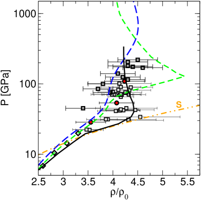
Obviously, the theoretical hydrogen EOSs differ substantially from each other. Along the Hugoniot states, the Sesame EOS, which precedes even the gas gun data, is relatively stiff at Mbar but the most compressible one at Mbars. Conversely, the ab initio H EOS is relatively compressible below 1 Mbar compared to the Sesame and SCvH-i EOS, and to the spherical-shock compression data, with a maximum compressibility at Mbar where dissociation occurs. At higher pressures of 1 to 3 Mbar, the ab initio EOS runs nearly through the experimental central values which indicate a low compression ratio of 4.25, whereas SCvH-i EOS agrees well with the data up to 0.8 Mbars but then turns to a large maximum compressibility at Mbar where in the underlying SCvH-ppt EOS the plasma phase transition occurs. These properties lead to systematic differences in the resulting Saturn models.
3 Results
3.1 Structure models with different equations of state
In this Section we focus on the effect of the different EOSs (Sesame, SCvH, LM-REOS) on the resulting Saturn models. The presented models have been calculated for , 10h 39m, and the default values of the other observational constraints as given in Table 1. Figure 2 shows the results.
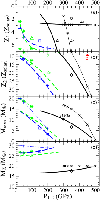
For each of the considered mantle EOS, the parameters , , , and behave similarly with . The deeper the layer boundary, the higher become and and, as a response, the lower becomes , while remains nearly constant within . Zero-core mass models are possible simply by putting the layer boundary sufficiently deep into the planet. The maximum core mass is determined by the condition that neither nor must become negative. It is for rocky cores and about for water cores.
For given , water cores are up to 50% heavier than rock cores because low-density material requires a larger volume. Displaced envelope material must be replaced by core material, hence the core becomes heavier. Note that water core models that approach the limit have been computed for LM-REOS mantle EOS only, but they exist for the other mantle EOS as well.
The core mass responds weakly to the surface temperature. The found slight decrease by can intuitively be explained by the colder and thus denser envelopes. However, the colder outer envelope requires less heavy elements to match , but up to more heavy elements in the inner envelope. Thus the found insensitivity of , and also of , to the surface temperature appears to be a more complex compensation of different effects in Saturn.
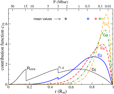
The general behavior of the solutions can be understood with the help of Figure 3. It shows the sensitivity of the gravitational moments to the internal mass distribution as parameterized by the contribution functions , see Eq. (2). While they have been computed for a particular model, i.e. the LM-REOS based Saturn model S12-3a as highlighted in Figure 2c, their properties are the same for all three-layer models. As it is well knowm (Zharkov and Trubitsyn, 1978) the higher the order of the gravitational harmonic, the farther out are the locations of mean and maximum sensitivity and the more pronounced is the latter one. and are most sensitive at pressures of and Mbar, respectively. At the 1 Mbar level, the sensitivity of has dropped to % of its maximum value. is almost insensitive to the mass below 3 Mbars, a typical pressure for the outer/inner envelope boundary of LM-REOS based Saturn models. Therefore, changes little with for Mbar. As the sensitivity of is similar to that of and just slightly shifted to higher pressures, the computed value is affected by the value of as well. But because is to be adjusted by the value, i.e. by the mass distribution interior to where its sensitivity is low, small changes in for adjustment require strong changes in , see Figure 2b.
LM-REOS based models
Using LM-REOS, we find solutions for Mbars. For all of these models, is nearly constant no matter what the values of and are. This is because with the layer boundary so deep inside, is little sensitive to the mass distribution there. As , in contrast, covers a wide range of 0–60%, there are solutions with , unlike for Jupiter (Nettelmann et al., 2012).
For LM-REOS based models the layer boundary has to be put rather deep inside the planet in order to nearly suppress the influence of the matter interior to to the values of and . Otherwise, say for Mbar, the rise in could no longer be compensated for by a lower value because already goes to zero. This behavior is a direct consequence of the higher compressibility of the H EOS at sub-Mbar pressures (Figure 1).
The total mass of heavy elements is 16–, less than predicted for Jupiter with LM-REOS (, Nettelmann et al., 2012). However, Saturn’s corresponds to an overall enrichment –15 , higher than Jupiter’s ().
Sesame based models
Sesame EOS based models have the layer boundary between 0.2 and 2.5 Mbar. With Mbar, the sensitivity of rises strongly (Figure 3) so that has to decrease rapidly in order to not produce too high values. There is no overlap of the functions and , i.e. Sesame EOS based Saturn models require a higher metallicity in the inner than in the outer envelope. Because of the stiffness of the H-Sesame EOS up to 1 Mbar (Figure 1), the layer boundary can be farther out and the values as well as the total mass of heavy elements can be up to 2.5 times higher than for LM-REOS based models. In fact, the layer boundary must be farther out because the rise in for increasing is accompanied by a rapid decrease in , which must not become negative, a direct effect of the higher compressibility of the H-Sesame EOS at higher pressures up to 10 Mbar (Figure 1).
SCvH-i based models
From the gross compressibility behavior of the Hugoniot up to 100 GPa one would expect the SCvH-i EOS based solutions to fall between those for the other two EOSs. This in fact happens with respect to the parameters , , and . In particular, the just slightly higher compressibilities of SCvH-i compared to Sesame EOS below 100 GPa suggest just slighty lower values than for that EOS. However, the values are relatively higher than for the Sesame EOS based models. This can only be due to higher temperatures along the SCvH-i Saturn adiabat, as higher temperatures at given pressure level reduce the mass density, which allows for more heavy elements to be added. We will encounter the same argument again in Section 3.2. In contrast to SG04, we do not find models with . Presumably, this stems from the application of the more recent, accurate data.
Both Sesame and SCvH-i EOS based models have –, a similar amount as Jupiter may have (–; SG04). With –, this is a larger enrichment than in comparable models for Jupiter (3–8 ). Note that SG04 use an earlier value .
Internal profiles
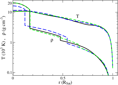
For each of the EOS, one selected interior profile is shown in Figure 4. The temperatures along the SCvH-i Saturn adiabat in the outer envelope are indeed higher than for the Sesame adiabat. For the LM-REOS based adiabat, the onset of dissociation occurs at where the temperature gradient flattens. A typical value of the density is 2 g cm-3 in the inner envelope, 15 g cm-3 in a rocky core, and 8 g cm-3 in a water core, while in the outer envelope the density changes by four orders of magnitude.
Concluding, for each of the considered EOS, similar values of the metallicity in the outer envelope (e.g., solar), in the inner envelope (e.g. 10– solar), and of the core (e.g., 0– for rocky or 0– for water cores) are possible. It depends mainly on the position of an internal compositional gradient (for instance in form of a layer boundary), which values are adopted. In contrast, the different EOSs require different locations of that gradient, and LM-REOS predicts a lower total mass of heavy elements than the other two EOSs.
3.2 LM-REOS based structure models with different helium abundances, rotation rates, and values
The resulting atmospheric heavy element enrichment of solar of the LM-REOS based Saturn models is rather low compared to the measured carbon enrichment of solar. Therefore, we investigate in this Section qualitatively the effect of the assumed atmospheric helium abundance, of the rotation rate, and of the value on the resulting outer envelope metallicity. As we are aiming to get higher values than for the models in Section 3.1, we only consider higher values, up to the observational uncertainty (any increases with the mass density in the sensitive region), lower values ( decreases linearly with ) of respectively 0.16 and 0.1; but we consider a higher rotation rate (to face a possible reality), although it will require a reduction in the heavy element content of the outer part of a planet. For all of these models, the transition pressure is at 300 GPa and the core consists of rocks. At temperatures between 140 and 300 K, the analytic Van-der-Waals-gas EOS is used for H2 and He, and the ideal gas EOS for molecular H2O, but this has no relevant effect on the resulting adiabats.
Figure 5 shows the resulting enrichment factors for the metallicity in the outer envelope –to be compared with the (potentially) measured abundances– and also in the inner envelope.
Obviously, the influence of on is weak. Only for extremely high values of the effect becomes of same size as the effect of a slower rotation by 7 minutes, which is . Note that constitutes a reather big amplification of the 1% relative uncertainty in the rotation rate.
In case a high rotation rate of 10h 32m should proof true, the heavy element enrichment would decrease down to solar for a helium abundance . Note that we do not adjust the planet radius to the rotation rate. Interestingly, the rotation rate mainly affects the inner envelope metallicity. This can be explained by the response of on a change in and as described in B.
The biggest effect on can be achieved by lowering the helium abundance, where of heavy elements can be added for of helium. It is because the less helium there is, the higher the specific heat of the material, and thus the lower must be the temperature along the adiabat to keep the entropy constant. Colder adiabats give denser envelopes and thus allow for less heavy elements to be put into.
Despite the wide range of considered parameter values, with the possible atmospheric heavy element abundance remains clearly below the 9fold enrichment of carbon. Our LM-REOS based models therefore predict O/H to be less than solar.
3.3 Moment of Inertia
Helled (2011) showed that an observational determination of Saturn’s axial moment of inertia, would impose an additional constraint on Saturn’s core mass, and that the necessary measurements can be provided by the Cassini extended extended mission. Figure 6 presents our results for Saturn’s nondimensional moment of inertia, for a representative subset of the models of Fig. 2. As pointed out by and in agreement with Helled (2011), we find different values for different core mass values for models that all meet the observed and values within their tight bounds. In particular, for a fixed core EOS (rocks or water) and mantle EOS (SCvH, Sesame, or LM-REOS), and not too small core mass values (), the relation between and becomes unique. However, due to the uncertainties in the core and envelope EOS, a measurement of could further, but not unambiguously constrain the core mass. Moreover, our physical EOS based, adiabatic models yield a very narrow possible range for , that even does not overlap with the prediction by Helled (2011), see Figure 6b. Therefore, a measured value would definitely be of great value for discriminating between competing Saturn models.
As moment of inertia measurements for gas giant planets are challenging, the Radau-Darwin approximation is often used for an estimate. It expresses in terms of the easier accessible and the expansion parameter , and becomes exact only in the limit of constant density bodies. Using km, , and the values of Table 1, we calculate (solid arrow in Figure 6b). The more consistent values of Table 1 in Helled (2011) suggest (dashed arrow in Figure 6b). Interestingly, our interior model based values are higher than indicating that higher-order deformations () play a non-negligible role in the internal mass distribution. Note111modified after acceptance of this paper that different scalings of by either the equatorial radius as in Helled (2011) (R. Helled, pers.comm. 2013), or by the mean radius changes the value of Saturn’s by 7.2%.
3.4 Homogeneous Evolution
Homogeneous evolution implies a constant mean molecular weight in every mass shell of the planet with time, while inhomogeneous evolution also allows for vertical mass transport such as He rain or core erosion. In the considered case of homogeneous evolution, we get cooling times of 2.56 Gyr for the LM-REOS model, 2.36 Gyr (SCvH-i EOS model), and 2.31 Gyr (Sesame EOS model).
Neglecting the three contributions from angular momentum conservation, change of the energy of rotation, and from the time-dependence of the irradiation yields 0.05 Gyr longer cooling times for Saturn. While with Gyr, the cooling time comes out significantly shorter than the age of the solar system of 4.56 Gyr —commonly believed to also be the age of the planets within an uncertainty of a few Myr according to circumstellar disk observations (Strom et al., 1993)— it is in agreement with previous calculations. For instance, using the SCvH-i EOS, Guillot et al. (1995) compute Gyr and Fortney and Hubbard (2003) 2.1 Gyr for an adiabatic, homogeneously evolving Saturn.
Our results show once more that the short cooling time of a homogeneously evolving Saturn is essentially independent on details of the model assumptions such as the size of the core. In other words, we confirm the well-known evidence for a real excess luminosity compared to the predicted luminosity from homogeneous evolution (Pollack et al., 1977; Saumon et al., 1992; Fortney and Hubbard, 2003).
4 Summary and Discussion
4.1 Gross features
We have applied different EOSs to compute structure and evolution models for Saturn within the standard approach of a layered interior with only few layers that cool down homogeneously with time. Because of the large applied input parameter space we have selected combinations of parameters that we believe yield a reliable estimate of the overall uncertainty in key internal structure parameters. In particular, with LM-REOS and assuming and 10h 39m we find –, –, solar, and 2.6 Gyr; with Sesame-EOS we find –, solar, –, and 2.3 Gyr, while SCvH EOS based models have values in between. The value of of the LM-REOS based models can be lifted up to a factor of two if is lowered down to 0.10. With –2.6 Gyr, the cooling time is significantly shorter than the age of the solar system, pointing to a failure of the cooling model that is to be sought beyond the uncertainties in Saturn’s composition or the EOS.
We encourage measurements of Saturn’s moment of inertia and of the atmospheric abundance of helium and oxygen for discriminating between the wide range of possible Saturn models and for probing the underlying EOS in certain pressure ranges.
4.2 O:H ratio
The O:H ratio could in principle be derived from brightness temperature measurements at m wavelengths using LOFAR (D. Gautier, pers. comm.), which is a set of ground-based radio antennas in western Europe. From a measured O:H, in addition to the already measured C:H, the atmospheric metallicity can be estimated and compared with the values of the Saturn structure models. For this purpose, we show possible O:H– relations in Fig. 7. For a given O:H, has been computed as the sum of the heavy element particle abundances times their atomic weight, divided by the sum over all element abundances times their weight, where we assume He:H = 0.052 (), C:H solar, and (or , ) solar abundances of the elements {N, P, S, Ne, Ar, Kr, Xe, Mg, Al, Ca}, using the solar system abundances of Lodders (2003). As Jupiter’s atmosphere is observed to be strongly depleted in Ne, which may also be the case for Saturn if caused by He sedimentation (Wilson and Militzer, 2010), we also compute with Ne:H=0.
Obviously, models with would imply a low O:H of only 2x solar; , the upper limit of the LM-REOS based Saturn models, would imply O:H = 6–8 solar. Higher values are possible with the Sesame or the SCvH-i EOS. Concluding, a measured O:H could tremendously help to discriminate between the various Saturn models.

4.3 Core mass and formation
The possible core mass values of Jupiter and Saturn persistently attract attention, as the hope to infer the planet formation process from the ”face value” of the present core mass continues to exist. Leading candidates for possible formation processes are the core accretion scenario, where the gaseous envelope is accreted onto a heavy-element core (Alibert et al., 2005; Dodson-Robinson et al., 2010; Kobayashi et al., 2012), and the gravitational disk instability scenario, where the planet would form through self-contraction of a gaseous cloud (Helled and Schubert, 2008, e.g.).
Let us assume the initial core mass of Saturn was . What could that tells us? Such a heavy core exceeds the maximum core mass of found by Helled and Schubert (2008) and thus would rule out a disk-instability-kind formation for Saturn. On the other hand, it would allow for a comfortably short time scale for core accretion formation (Dodson-Robinson et al., 2010; Kobayashi et al., 2012), even for a non-zero abundance of grains in the protoplanetary envelope (Dodson-Robinson et al., 2010).
If the initial core mass of Saturn was , then both formation processes could have let to the present Saturn. Given Saturn’s high total heavy element mass of 16–30, disk-instability formation would indicate a massive protosolar disk (Helled and Schubert, 2009), as well as an early presence of planetesimals before formation was completed (Helled and Schubert, 2008).
In the case of an initial core mass of , again both scenarios could be possible. Here, core accretion formation would require the absence of grains in the envelope in order to reduce the gas pressure induced by warm temperatures in an opaque medium (Hori and Ikoma, 2010).
As main paths toward better constrained core mass properties, we support Helled’s (2011) suggestion of a moment of inertia measurement, and emphasize the need for a better understanding of Saturn’s envelope structure.
4.4 Three-layer models and helium rain in Saturn
The over and over confirmed finding of a too short cooling time for homogeneously evolving Saturn models, regardless of details in the structure models, or of the underlying EOS used, and the simultaneously repeated mentioning of a high likelihood for an inhomogeneously evolving Saturn as a result of He sedimentation (e.g., Pollack et al., 1977; Stevenson and Salpeter, 1977; Saumon et al., 1992; Guillot et al., 1995; Fortney and Hubbard, 2003) cast doubt on the usefulness of Saturn models that ignore this process.
The most recent theories of H/He phase separation predict demixing under relevant planetary conditions to occur when hydrogen metallizes under high pressures while the helium atoms are still neutral (Morales et al., 2009; Lorenzen et al., 2009, 2011). In Jupiter, metallization occurs rather far out in the planet at where the pressure is only 0.5 Mbar (French et al., 2012), but the lowest pressure that could be achieved in H/He demixing calculations so far is 1 Mbar (Lorenzen et al., 2011). Indeed, the ab initio data based H/He phase diagram suggests demixing in Saturn at least within 1–5 Mbar (Lorenzen et al., 2011), which corresponds to the region beneath . Let us thus divide Saturn’s mantle into three regions: an outer region down to 1 Mbar (), an innermost helium-rich region where the sedimented helium dissolves again in its surrounding, possibly a helium-layer (Fortney and Hubbard, 2003), and a middle region where the conditions favor H/He phase separation.
In the middle region, the helium abundance at given will reduce until the remaining He atoms become miscible: the helium abundance will follow the demixing curve (Stevenson and Salpeter, 1977). In –-space, such an inhomogeneous region could simply be described by a smoothed layer boundary. In –-space, the effect of an inhomogeneity could be significant, as it may be correlated with a strongly superadiabatic temperature gradient (Stevenson and Salpeter, 1977), which would require higher envelope metallicities and affect the derived core mass (Leconte and Chabrier, 2012). Also important may be the induced differential rotation from sinking droplets that conserve their angular momentum. Cao et al. (2012) showed that a tiny differential rotation would suffice to drive the magnetic field and explain its observed dipolarity.
In case the sedimented helium dissolves in the lower region, that part is well represented by an inner envelope with enhanced abundance as in our models. But in case the helium rains down to the core, a preferred solution to explain Saturn’s high luminosity (Fortney and Hubbard, 2003), the upper part of what we count to be core material may in fact be helium. Thus, Saturn’s maximum core mass could be lower than predicted by our models.
In the outer region we would mainly see the depletion in helium, because helium atoms from the upper regions are transported repeatedly by convection down into the immiscibility region, where a fraction of them gets lost into the deep through sedimentation. Whatever happens to the compositional and temperature gradient deep in the planet, the outer, miscible envelope should remain homogeneous and adiabatic. Therefore, our results for the atmospheric helium and heavy element abundances are certainly caused or influenced by He-sedimentation, but are not expected to alter when He sedimentation would be explicitly accounted for.
4.5 Why would we expect a (dis)continuous heavy element distribution?
Standard three-layer models with heavy element discontinuity benefit from two additional parameters (, ) that can be used to fit the observational constraints. However, those models would even more benefit from a physical justification. At least, the assumption of a sharp layer boundary between two convective, homogeneous layers offers the advantage of a self-consistent picture, where upward particle transport across would be inhibited but not necessarily the heat transport. In contrast, a continuous, inhomogeneous heavy element distribution as suggested by Leconte and Chabrier (2012) might lead to a semi-convective boundary layer with reduced heat transport. Whether such a picture can explain the luminosities of both Jupiter and Saturn remains to be shown.
A possible origin for an inhomogeneous heavy element distribution could be the erosion of an initially big core, with subsequent small-scale layer formation with small compositional gradients (Leconte and Chabrier, 2012), and finally merging of the layers to a single one as seen in hydrodynamic simulations of fluids with both temperature and compositional gradients (Wood et al., 2012). Thus, a high, homogeneous metallicity in the inner envelope could be the result of an eroded core where the core material went through stages of layer merging until the compositional gradient got large enough to stop merging with what we now see as an outer envelope.
4.6 Summarized main findings
-
1.
The H/He EOS strongly influences the atmospheric metallicity, and the possible position of an internal layer boundary, but has little influence on the core mass and the cooling time. We find – and Gyr.
-
2.
The total mass of heavy elements in Saturn can be less (LM-REOS) or equal (Sesame, SCvH-i EOS) to that in Jupiter, while the averaged enrichment is larger than that of comparable Jupiter models.
-
3.
Our LM-REOS based Saturn models predict solar () for an atmospheric helium abundance () by mass. The corresponding predicted maximum O:H ratio is solar ().
-
4.
For Saturn, we calculate a non-dimensional axial moment of inertia to 0.236.
We thank Daniel Gautier for illuminating conversations on abundance measurements, Johannes Wicht and Ravit Helled for interesting discussions, Andreas Becker for computing the high-temperature extension of the H-REOS.2 Hugoniot curve, and Winfried Lorenzen for discussions on H-He demixing. The work presented in this paper is supported by the ”Deutsche Forschungsgemeinschaft” (DFG) within the SFB 652 and the project RE 882/11.
References
- Alibert et al. (2005) Alibert, Y., Mousis, O., Mordasini, C., Benz, W., 2005. New Jupiter and Saturn formation models meet observations. ApJ 626, L57.
- Anderson and Schubert (2007) Anderson, J., Schubert, G., 2007. Saturn’s Gravitational Field, Internal Rotation, and Interior Structure. Science 317, 1384–1387.
- Atreya et al. (2003) Atreya, S. K., Mahaffy, P. R., Niemann, H. B., Wong, M. H., Owen, T. C., 2003. Composition and origin of the atmosphere of Jupiter—an update, and implications for the extrasolar giant planets. Planet. Space Sci. 51, 105.
- Boley et al. (2011) Boley, A. C., Helled, R., Payne, M. J., 2011. The heavy element composition of disk instability planets can range from sub- to super-nebular. ApJ.
- Boriskov et al. (2005) Boriskov, G. V., Bykov, A. I., Ilkaev, R., Selemir, V. D., Simakov, G. V., Trunin, R. F., Urlin, V. D., Shuikin, A. N., Nellis, W. J., 2005. Shock compression of liquid deuterium up tp 109 GPa. Phys. Rev. B 71, 092104.
- Campbell and Anderson (1989) Campbell, J. K., Anderson, J. D., 1989. Gravity field of the Saturnian system from Pioneer and Voyager tracking data. Astronom. J. 97, 1485.
- Cao et al. (2012) Cao, H., Russell, C. T., Wicht, J., Christensen, U. R., Dougherty, M. K., 2012. Saturn’s high-degree magnetic moments: Evidence for a unique planetary dynamo. Icarus 221, 388–394.
- Conrath and Gautier (2000) Conrath, B., Gautier, D., 2000. Saturn Helium Abundance: A Reanalysis of Voyager Measurements. Icarus 144, 124.
- Conrath et al. (1984) Conrath, B. J., Gautier, D., Hanel, R. A., Hornstein, J. S., 1984. The helium abundance of Saturn from Voyager measurements. Astrophys. J 282, 807–815.
- Desch and Kaiser (1981) Desch, M. D., Kaiser, M. L., 1981. Voyager measurement of the rotation period of Saturn’s magnetic field. Geophys. Res. Lett. 8, 253.
- Dodson-Robinson et al. (2010) Dodson-Robinson, S., Bodenheimer, P., Laughlin, G., Willacy, K., Turner, N. J., Beichman, C. A., 2010. Saturn forms by core accretion in 3.4 Myr. ApJ 688, L99.
- Fletcher et al. (2009) Fletcher, L. N., Orton, G., Teanby, N., Irwin, P., Bjoraker, G., 2009. Methane and its isotopologues on Saturn from Cassini/CIRS observations. Icarus 199, 351–367.
- Fortney and Hubbard (2003) Fortney, J. J., Hubbard, W. B., 2003. Phase Separation in Giant Planets: Inhomogeneous evolution of Saturn. Icarus 164, 228.
- Fortney et al. (2011) Fortney, J. J., Ikoma, M., Nettelmann, N., Guillot, T., Marley, M. S., 2011. Self-consistent Model Atmospheres and the Cooling of the Solar System Giant Planets. ApJ 729, 32.
- French et al. (2012) French, M., Becker, A., Lorenzen, W., Nettelmann, N., Bethkenhagen, M., Wicht, J., Redmer, R., 2012. Ab initio simulations for material properties along the Juptier adiabat. ApJS 202, A5.
- French et al. (2009) French, M., Mattsson, T. R., Nettelmann, N., Redmer, R., 2009. Equation of state and phase diagram of water at ultrahigh pressures as in planetary interiors. Phys. Rev. B 79, 054107.
- Guillot (1999) Guillot, T., 1999. A comparison of the interiors of Jupiter and Saturn. Planet. Space Sci. 47, 1183.
- Guillot et al. (1995) Guillot, T., Chabrier, G., Gautier, D., Morel, P., 1995. Effect of radiative transport on the evolution of Jupiter and Saturn. ApJ 450, 463.
- Guillot and Gautier (2007) Guillot, T., Gautier, D., 2007. The Giant Planets. In: Schubert, G., Spohn, T. (Eds.), Treatise of Geophysics, vol. 10, Planets and Moons. Amsterdam: Elsevier, p. 439 (arXiv:0912:2019).
- Gurnett et al. (2007) Gurnett, D. A., Persoon, A. M., Kurth, W. S., Groene, J. B., Averkamp, T. F., Dougherty, M. K. andSouthwood, D. J., 2007. The Variable Rotation Period of the Inner Region of Saturn’s Plasma Disk. Science 316, 442–445.
- Helled (2011) Helled, R., 2011. Constraining Saturn’s core properties by a measurement of ots moment of inertia-implications to the Cassini Solstice Mission. ApJ 735, L16.
- Helled et al. (2010) Helled, R., Bodenheimer, P., Lissauer, J. J., 2010. Composition of massive planets. Proceeding IAU symp. 276, 119.
- Helled and Schubert (2008) Helled, R., Schubert, G., 2008. Core formation in gaseous protoplanets. Icarus 0, 0.
- Helled and Schubert (2009) Helled, R., Schubert, G., 2009. Heavy element enrichement of a Jupiter-mass protoplanet as a function of orbital distance. ApJ 697, 1256.
- Helled et al. (2009a) Helled, R., Schubert, G., Anderson, J. D., 2009a. Empirical models of pressure and density in Saturn s interior: Implications for the helium concentration, its depth dependence, and Saturn s precession rate. Icaus 199, 368–377.
- Helled et al. (2009b) Helled, R., Schubert, G., Anderson, J. D., 2009b. Jupiter and Saturn Rotation Periods. Planet. Space Sci. 57, 1467–1473.
- Holst et al. (2012) Holst, B., Redmer, R., Gryaznov, V. K., Fortov, V. E., Iosilevskiy, I. L., 2012. Hydrogen and helium in shock wave experiments, ab initio simulations and chemical picture modeling. Eur. Phys. J. D 66, 104.
- Hori and Ikoma (2010) Hori, Y., Ikoma, M., 2010. Critical core masses for gas giant formation with grain free-envelopes. ApJ 714, 1343.
- Hubbard (1999) Hubbard, W. B., 1999. Gravitational Signature of Jupiter’s Deep Zonal Flows. Icarus 137, 357–359.
- Hubbard and Marley (1989) Hubbard, W. B., Marley, M. S., 1989. Optimized Jupiter, Saturn, and Uranus interior models. Icarus 78, 102.
- Jacobson et al. (2006) Jacobson, R. A., Antresian, P. G., Bordi, J. J., Criddle, K. E., Ionasescu, R., Jones, J. B., Mackenzie, R. A., Meek, M. C., Parcher, D., Pelletier, F. J., 2006. The gravity field of the Saturnian system from satellite observations and spacecraft tracking data132. Astronom. J. 132, 2520.
- Kerley (2003) Kerley, G., 2003. Equations of state for hydrogen and deuterium. Tech. rep., SANDIA REPORT, SAND2003-3613.
- Kerley (2004a) Kerley, G., 2004a. Structures of the planets Jupiter and Saturn. Tech. rep., Kerley Tech. Services, Report KTS04-1.
- Kerley (2004b) Kerley, G., 2004b. An Equation of State for Helium. Tech. rep., Kerley Tech. Services, Report KTS04-2.
- Knudson and Desjarlais (2009) Knudson, M. D., Desjarlais, M. P., 2009. Shock Compression of Quartz to 1.6 TPa: Redefining a Pressure Standard. Phys. Rev. Lett. 103, 225501.
- Knudson et al. (2004) Knudson, M. D., Hanson, D. L., Bailey, J. E., Hall, C. A., Asay, J. R., Deeney, C., 2004. Principal Hugoniot, Reveberating Wave, and mechanical reshock measurement of liquid deuterium to 400 GPa using plate impact techniques. Phys. Rev. B 69, 144209.
- Kobayashi et al. (2012) Kobayashi, H., Ormel, C. W., Ida, S., 2012. Rapid formation of Saturn after Jupiter completion. ApJ submitted.
- Leconte and Chabrier (2012) Leconte, J., Chabrier, G., 2012. A new vision on giant planet interiors: the impact of double-diffusive convection. A&A 540, A20.
- Lindal et al. (1985) Lindal, G., Sweetnam, D. N., Eshleman, V. R., 1985. The atmosphere of Saturn: an analysis of the Voyager occultation measurements. Astronom. J. 90, 1136.
- Lodders (2003) Lodders, K., 2003. Solar System Abundances and Condensation Temperatures of the Elements. ApJ 591, 1220.
- Lorenzen et al. (2009) Lorenzen, W., Holst, B., Redmer, R., 2009. Demixing of Hydrogen and Helium at Megabar Pressures. Phys. Rev. Lett. 102, 5701.
- Lorenzen et al. (2011) Lorenzen, W., Holst, B., Redmer, R., 2011. Metallization in hydrogen-helium mixtures. Physical Review B 84, 235109.
- Lyon and Johnson (1992) Lyon, S., Johnson, J. D. e., 1992. Sesame: Los alamos national laboratory equation of state database. Tech. rep., LANL report no. LA-UR-92-3407.
- Miller and Fortney (2011) Miller, N., Fortney, J. J., 2011. The heavy-element masses of extrasolar giant planets, revealed. ApJ 736, L29.
- Mizuno (1980) Mizuno, H., 1980. Formation of the giant planets. Prog. Theo. Phys. 64, 544.
- Morales et al. (2009) Morales, M. A., Schwegler, E., Ceperley, D., Pierleoni, C., Hamel, S., Caspersen, K., 2009. Phase separation in hydrogen-helium mixtures at Mbar pressures. PNAS 106, 1324–1329.
- Nellis et al. (1983) Nellis, W. J., Mitchell, A. C., van Thiel, M., Devine, G. J., Trainor, R. J., Brown, N., 1983. EOS data for molecular H and D at shock pressures in the range 2-76 GPa. J. Chem. Phys. 79, 1480.
- Nettelmann et al. (2012) Nettelmann, N., Becker, A., Holst, B., Redmer, R., 2012. Jupiter models with improved hydrogen EOS (H-REOS.2). ApJ 750, A52.
- Nettelmann et al. (2011) Nettelmann, N., Fortney, J., Kramm, U., Redmer, R., 2011. Thermal evolution and structure models of the transiting super-Earth GJ1214b. ApJ 750, A52.
- Nettelmann et al. (2008) Nettelmann, N., Holst, B., Kietzmann, A., French, M., Redmer, R., Blaschke, D., 2008. Ab initio equation of state data for hydrogen, helium, and water and the internal structure of Jupiter. ApJ 683, 1217.
- Orton and Ingersoll (1980) Orton, G. S., Ingersoll, A. P., 1980. Saturn’s atmospheric temperature structure and heat budget. J. Geophys. Res. 85, 5871.
- Pollack et al. (1977) Pollack, J. B., Grossman, A. S., Moore, R., Graboske, H. C., 1977. A calculation of Saturn’s gravitational contraction history. Icarus 30, 111–128.
- Saumon et al. (1995) Saumon, D., Chabrier, G., ”van Horn”, H. M., 1995. An equation of state for low-mass stars and giant planets. ApJS 99, 713.
- Saumon and Guillot (2004) Saumon, D., Guillot, T., 2004. Shock Compression of Deuterium and the Interiors of Jupiter and Saturn. ApJ 609, 1170.
- Saumon et al. (1992) Saumon, D., Hubbard, W. B., Chabrier, G., van Horn, H. M., 1992. The role of the molecular-metallic transition of hydrogen in the evolution of Jupiter, Saturn, and brown dwarfs. ApJ 391, 827–831.
- Stevenson and Salpeter (1977) Stevenson, D. J., Salpeter, E. E., 1977. The dynamics and helium distribution in hydrogen-helium fluid planets. ApJS 35, 239–261.
- Strom et al. (1993) Strom, S. E., Edwards, S., Skrutskie, M. F., 1993. Evolutionary time scales for circumstellar disks associated with intermediate- and solar-type stars. In: Levy, E. H., Lunine, J. I. (Eds.), Protostars and Planets III. Amsterdam: Elsevier, pp. 837–866.
- von Zahn et al. (1998) von Zahn, U., Hunten, D. M., Lehmacher, G., 1998. Helium in Jupiter’s atmosphere: Results from the Galileo probe helium interferometer experiment. J. Geophys. Res. 103, 22815.
- Wilson and Militzer (2010) Wilson, H. F., Militzer, B., 2010. Sequestration of noble gases in giant planet interiors. Phys. Rev. Lett. 104, 121101.
- Wood et al. (2012) Wood, T. S., Garaud, P., Stellmach, S., 2012. A new model for mixing by double-diffusive convection (semi-convection). II. The transport of heat and composition through layers. arXiv:1212.1218v1 [astro-ph].
- Zharkov and Trubitsyn (1978) Zharkov, V. N., Trubitsyn, V. P., 1978. Physics of Planetary Interiors. Tucson, AZ: Parchart.
Appendix A Erratum Jupiter-paper
In the Jupiter-II paper by Nettelmann et al. (2012) on Jupiter structure and homogeneous evolution models it was stated that including the energy of rotation in the thermal evolution leads to a reduced luminosity with time and thus a longer cooling time. The latter statement must be corrected for a shorter cooling time: the energy of rotation will not be released by radiation at a later time. Therefore, Jupiter’s cooling time is decreased by 0.2 Gyr (and not prolonged by 0.2 Gyr as stated in that paper). The given final value for cooling time of 4.41 Gyr, when in addition the time-dependence of is included, remains valid.
Appendix B Estimate as a function of
We here derive an estimate for the necessary change in in response to a change when is to be kept unchanged. According to Equation 1 we can approximate by
| (7) |
where , , is the mean density of layer No. , and its volume. The contribution from the small, central core is neglected. According to the additive volume law for mixtures we can write and thus
| (8) |
so that and . Because the value of is an observational constraint, must be zero under the perturbations and . With Equations (7) and (8) we thus have
| (9) |
hence
| (10) |
For a typical three-layer Saturn model as shown in Figure 4, , leading to , , , leading to , , leading to , and thus , in reasonable agreement with as seen in Figure 5.