Reducing Systematic Error in Cluster Scale Weak Lensing

Abstract

Weak lensing provides an important route toward collecting samples of clusters of galaxies selected by mass. Subtle systematic errors in image reduction can compromise the power of this technique. We use the B-mode signal to quantify this systematic error and to test methods for reducing this error. We show that two procedures are efficient in suppressing systematic error in the B-mode: (1) refinement of the mosaic CCD warping procedure to conform to absolute celestial coordinates and (2) truncation of the smoothing procedure on a scale of 10^′. Application of these procedures reduces the systematic error to 20% of its original amplitude. We provide an analytic expression for the distribution of the highest peaks in noise maps that can be used to estimate the fraction of false peaks in the weak lensing $\kappa$-S/N maps as a function of the detection threshold. Based on this analysis we select a threshold S/N = 4.56 for identifying an uncontaminated set of weak lensing peaks in two test fields covering a total area of $\sim 3$deg². Taken together these fields contain seven peaks above the threshold. Among these, six are probable systems of galaxies and one is a superposition. We confirm the reliability of these peaks with dense redshift surveys, x-ray and imaging observations. The systematic error reduction procedures we apply are general and can be applied to future large-area weak lensing surveys. Our high peak analysis suggests that with a S/N threshold of 4.5, there should be only 2.7 spurious weak lensing peaks even in an area of 1000 deg² where we expect $\sim$ 2000 peaks based on our Subaru fields.

1. Introduction

Weak lensing is a fundamental tool of modern cosmology. A weak-lensing map provides a weighted “picture” of the projected surface mass density and thus a route to identifying clusters of galaxies selected by mass (e.g. Miyazaki et al., 2002a; Dahle et al., 2003; Schirmer et al., 2003; Hetterscheidt et al., 2005; Wittman et al., 2006; Gavazzi & Soucail, 2007; Miyazaki et al., 2007; Shan et al., 2012). Subtle issues limit the application of weak lensing maps as sources of cluster catalogs. A serious astrophysical limitation is the projection of large-scale structure along the line-of-sight (see e.g. White et al., 2002; Hamana et al., 2004, 2012). An observational limitation is the presence of systematic errors in the maps (Geller et al., 2010; Kurtz et al., 2012) . Here we focus on a method of reducing these errors.

Wittman et al. (2001) and Miyazaki et al. (2002a) first identified rich clusters from weak lensing maps. Since then larger and larger weak lensing surveys with increasingly sophisticated reduction techniques have led to a steep increase in the number of clusters initially detected in weak lensing maps (Hetterscheidt et al., 2005; Wittman et al., 2006; Schirmer et al., 2007; Gavazzi & Soucail, 2007; Miyazaki et al., 2007; Maturi et al., 2007; Bergé et al., 2008; Dietrich et al., 2007; Bellagamba et al., 2011; Shan et al., 2012). Shan et al. (2012) used the CFHT to carry out the largest area survey to date covering 64 deg². Among the 301 weak lensing peaks with signal-to-noise ratio greater than 3.5, only 126 have a corresponding brightest cluster galaxy within 3^′ of the weak lensing peak. Shan et al. (2012) conclude that many of the weak lensing peaks, even above this threshold, are probably noise.

In a detailed reanalysis of the 2.1deg² GTO field of Miyazaki et al. (2002a, 2007); Kurtz et al. (2012) show that the highest peak of the B-mode map (in this map the sources ellipticities are rotated by 45^∘ and there should be no signal) has signal-to-noise, S/N $\sim 4.25$ and there are four peaks in the B-mode map with S/N$>3.7$. It is interesting that Shan et al. (2012) find a similar number of high-significance peaks per unit area in their B-mode maps. Analysis of the B-mode map prompted Kurtz et al. (2012) to set their threshold for weak lensing cluster detection at 4.25. Above this threshold 2/3 of the weak lensing peaks correspond to individual massive clusters.

Here we investigate possible underlying sources of the high peaks in the B-mode maps. Our goal is reduction of the amplitude and frequency of these peaks as a basis for construction of more robust catalogs of weak lensing cluster detections. We apply our revised procedures to two fields observed with the Subaru Telescope: the GTO field of Miyazaki et al. (2002a, 2007) and a small portion of the DLS F2 field reobserved with Subaru.

In Section 2, we review the standard analysis of the Subaru imaging data. In Section 3 we review the construction of the galaxy catalog. In Section 4 we describe the basic weak lensing analysis we use. In Section 5 we develop a revised procedure for reducing systematics in the B-mode map. We demonstrate that there is excess power in the B-mode map on small and large scales relative to noise maps. Two procedures are effective in suppressing systematic in the B-mode map: (1) warping the image onto absolute sky coordinates and (2) introducing a large-scale (10^′) cutoff in the smoothing kernel applied to construct the weak lensing map. We define the weak lensing peaks and investigate thresholds in Section 6. In Section 7 we note some differences in our analysis of the GTO and DLS Subaru observations. Section 8 provides an analytic expression for the probability of finding the highest peak in the noise maps as spurious peaks in a weak lensing map. In Section 9 we test the lensing maps of our two fields by comparing the peaks with systems identified in dense redshift surveys. We demonstrate that a threshold S/N = 4.56 produces a robust catalog of peaks with few false positives.

Unless otherwise stated, we adopt the standard concordance cosmology $(h=0.72,\Omega_{m}=0.27,\Omega_{\Lambda}=0.73)$ and the AB magnitude system throughout this paper.

2. Imaging Data & Image Reduction

In this section we describe a revised reduction procedure that reduces systematic errors in weak lensing maps. As examples of the revised procedure, we use two regions imaged with Suprime-Cam on the Subaru Telescope (Miyazaki et al., 2002b). The GTO field covers $\sim 2$ deg², centered on (16:04, +43:12) and was observed by Miyazaki et al. (2002a). We re-observed the western $\sim 1$ deg² portion, (9:16, +30:00), of the Deep Lens Survey F2 field (DLS F2 Wittman et al., 2002). The new observations were taken in 0.75^′′ seeing. The GTO field consists of 9 Suprime-Cam pointings; the DLS observations consist of 4 Suprime-Cam pointings. Table 1 shows the numbering scheme for Subaru pointings in both the GTO and DLS fields.

We retrieved data from the SMOKA data archive server (Baba et al., 2002). These data satisfy the condition FILTER=W-C-RC and $\rm{PSF\_SIGMA}<0.9$ to obtain good image quality. $\rm{PSF\_SIGMA}$ is the typical FWHM (arcsec) of stellar images evaluated by SMOKA using SExtractor (Bertin & Arnouts, 1996). If the total exposure exceeds 2,000 seconds, we select frames with the smallest PSF_SIGMA and reject frames with larger PSF_SIGMA even if PSF_SIGMA is $\lesssim 0.9^{\prime\prime}$. As a result, we reject about 6 of 11, 10 of 15 and 1 of 5 exposures for GTO_0, GTO_4, and GTO_5, respectively. Table 1 gives the total exposure times, observation dates, filters, typical seeing, and effective limiting magnitude for each subfield. Imaging observation for the DLS F2 field were made with Suprime-Cam in January 1, 2008. Each of the 4 subfields is a 3600 sec exposures taken under stable seeing conditions. Table 1 lists the FWHM of the PSF on stacked images in each of the four subfields.

Table 1Observation Log.

Name	Ra	Dec	Exp. time (sec)	Observation date	Filter	Seeing	Limit mag
GTO_0	16:04:44.5	+43:11:12	2100	2001/4/23, 25	$R_{\rm C}$	0.66	25.38
GTO_1	16:07:39.0	+43:12:19	2400	2001/4/23, 25	$R_{\rm C}$	0.77	25.28
GTO_2	16:07:39.0	+43:37:37	1800	2001/4/23	$R_{\rm C}$	0.72	25.44
GTO_3	16:04:44.6	+43:36:30	1800	2001/4/24	$R_{\rm C}$	0.71	25.24
GTO_4	16:01:46.8	+43:37:37	2250	2001/4/24, 25, 5/18	$R_{\rm C}$	0.65	25.17
GTO_5	16:01:46.8	+43:12:19	2250	2001/4/24, 25	$R_{\rm C}$	0.70	24.90
GTO_6	16:01:46.8	+42:47:01	1800	2001/4/24, 25	$R_{\rm C}$	0.66	25.19
GTO_7	16:04:43.0	+42:47:01	1800	2001/4/25	$R_{\rm C}$	0.65	25.18
GTO_8	16:07:39.0	+42:47:01	1800	2001/4/25	$R_{\rm C}$	0.64	25.32
DLSF2_f0	09:16:30.9	+29:17:40	3600	2008/1/8	$i^{\prime}$	0.79	25.50
DLSF2_f1	09:16:31.0	+29:39:40	3600	2008/1/8	$i^{\prime}$	0.72	25.52
DLSF2_f2	09:16:31.0	+30:01:40	3600	2008/1/8	$i^{\prime}$	0.72	25.33
DLSF2_f3	09:16:31.0	+30:23:41	3600	2008/1/8	$i^{\prime}$	0.76	25.51

The basic image reduction follows Miyazaki et al. (2002a, 2007) and Kurtz et al. (2012). However, we make one major revision: we use independent astrometric data to register the images accurately with respect to the celestial coordinate while avoiding the introduction of any additional image warp.

The preliminary reduction of the raw image on each CCDs is standard. We use SExtractor to identify objects on the overscan-subtracted, flat-fielded, sky-subtracted image. We identify stellar objects from their easily identifiable linear size-magnitude relation. We manually select the stellar object catalog using this relation.

After completing the preliminary reduction, there are three additional steps in obtaining the final mosaic of stacked images; one of the steps is new. First we determine the accurate location of each CCD in instrument coordinates (Section 2.1). Second, we apply the image alignment warping procedure of Miyazaki et al. (2002a, 2007) (Section 2.2). Finally we introduce a new additional warp “Registration onto the celestial coordinate” (Section 2.3).

2.1. Solving the Basic Mosaic Geometry

We parameterize the accurate location of each CCD in instrument coordinates by the displacement and the rotation of each CCD $(\Delta x,\Delta y,\Delta\phi)_{\rm c}$, the telescope pointing offset between dithered exposures $(\Delta X,\Delta Y,\Delta\Phi)_{\rm e}$, and the optical distortion of the wide field corrector lens. The distortion parameters are well modeled by a 4th-order polynomial function:

$$\frac{R-r}{r}=ar+br^{2}+cr^{3}+dr^{4}$$ (1)

where $R$ and $r$ are distances from the optical axis in units of pixels on the CCD. $R$ is the original instrument coordinate and $r$ is the distortion-free coordinate.

To construct a mosaic we need a flux calibration to correct for the differences in sensitivity from chip to chip ($\Delta f_{c}$). These differences originate from differences in amplifier gain, differences in the normalization of flat fielding, and from corrections for the transmission of the atmosphere from exposure to exposure $\Delta f_{e}$. We derive this calibration by comparing the fluxes for unsaturated stars in overlapping regions of the frames. We call these parameters the “mosaicking rule”.

Operationally, we reduce the rotational component ($\Delta\phi,\Delta\Phi$) to the linearized form of the rotational matrix consisting of four components ( ($\phi_{ij}$), ($\Phi_{ij}$)) where $i,j\in(1,2)$. Because this matrix can treat not only rotation but also expansion, we include the first coefficient of the distortion parameter in this matrix. Varying the basic mosaic geometry parameters $(\Delta x,\Delta y,\phi_{ij},\Delta f)_{\rm c}$, $(\Delta X,\Delta Y,\Phi_{ij},\Delta f)_{\rm e}$, ($b,c,d$), we minimize

$$\Delta^{2}=\sum_{e>f}\sum_{i}^{\rm all~{}stars}\left(\frac{(\vec{\eta}_{i}^{(e)}-\vec{\eta}_{i}^{(f)})^{2}}{\sigma_{\eta}^{2}}+\frac{(f_{i}^{(e)}-f_{i}^{(f)})^{2}}{\sigma_{f}^{2}}\right)$$ (2)

where $\vec{\eta}_{i}^{(e)}$ and $f_{i}^{(e)}$ are the $e$-th exposure’s position in distortion-free coordinates and the corrected flux for $i$-th unsaturated star and $\sigma_{i},~{}i\in(\eta,f)$ are the typical error in the measurements of position and flux, respectively. We fix parameters for the first exposure of the series and the left bottom chip, i.e. $(\Delta x,\Delta y,\Delta\phi,\Delta f)_{\rm 0}=\vec{0}$, $(\Delta X,\Delta Y,\Delta\Phi,\Delta f)_{\rm 0}=\vec{0}$ as constraints.

This mosaicking rule is calculated by imcat (Kaiser et al., 1995). The best fit parameters are obtained by minimizing the positional difference of unsaturated control stars ($70\sim 100$ stars per CCD) for each exposure.

The residual alignment error in this procedure is $\sim 0.5$ pixel rms (0.1^′′), still large compared with typical distortions of the sources in weak lensing. Many stacking pipelines adopt this “typical stacking” warp only. We note that a typical stellar size is 0.6^′′; it should thus be possible to align the stellar positions to $\lesssim 0.06^{\prime\prime}$, one tenth of the stellar size. The accuracy of the “typical stacking” is insufficient and probably below the level that can be obtained from the data.

2.2. Jelly Focal Plane Warp

Residual positional differences from exposure to exposure in the typical stacking procedure in Section 2.1 may result from non-symmetric features of optical distortion (possibly due to imperfect optical alignment) not considered in the model. Differential atmospheric dispersion is another source of asymmetry.

We parameterize the residuals relative to one another by a polynomial function of the field position; we expect the residuals to be continuous over the field of view. The residuals are

$$\Delta\xi=\sum_{l=0}^{6}\sum_{m=0}^{l}a_{lm,e}\xi^{l-m}\eta^{m},\quad\Delta\eta=\sum_{l=0}^{6}\sum_{m=0}^{l}b_{lm,e}\xi^{l-m}\eta^{m}$$ (3)

where $\vec{\eta}=(\xi,\eta)$. We then obtain the coefficients $a_{lm,e}$ and $b_{lm,e}$ by minimizing the variance of the residuals. Each individual CCD image is “warped” using this polynomial correction prior to the stacking. This process reduces the alignment error to $\sim 0.05$ pixel (0.014^′′). Miyazaki et al. (2002a, 2007) and Kurtz et al. (2012) used this transformation following Kaiser et al. (1998). We refer to this transformation as “the original warp”, and we call the results of this warp “the original stacking”. The result is similar to Miyazaki et al. (2002a, 2007) and Kurtz et al. (2012).

2.3. Registration onto the Celestial Coordinate

The third transformation is new and we apply it as the final step in the reduction. The result of Section 2.2 is that all exposures except for the first one are registered on the first exposure with an accuracy of $\sim 0.05$ pixel, the tolerance we seek. However, there is no guarantee that the geometry of the first exposure is well matched to the celestial coordinate.

In practice, the absolute rotation of the instrument rotator is less well-known than its rotational angle relative to its zero point. There is no mechanical system to determine the zero point rotational angle for the rotator accurately for Suprime-Cam; the rotational angle relative to the origin is, however, very well known. The possibility of this zero point offset suggests that the final Suprime-Cam image will be rotated relative to the absolute celestial coordinate.

To align the final image with the celestial coordinate frame (not some artificial distorted frame, but a physical frame), we use an external catalog, USNO-A2.0 (Monet, 1998). This astrometric standard catalog has an accuracy of 0.4 arcsec although USNO-A2.0 is not deep enough to match the Suprime-Cam catalogs. The overlapping magnitude range includes moderately bright stars; these stars are saturated but do not have blooming pixels. It is thus difficult to measure their total intensity, but it is possible to measure their position because they have circular symmetry. We do not use the SDSS star catalog because it does not cover the enough of the sky to allow us to to extend our procedure outside the GTO field. We confirm that using the SDSS external astrometric catalog makes no significant difference in the warp relative to use of the USNO-A2.0.

In the same manner as the transformation in Section 2.2, we parameterise the residuals ($\Delta x,\Delta y$) of bright stars (they are slightly separated from the linear stellar sequence but have a comparable positional determination to the unsaturated stars provided there are no blooming pixels) in the first exposure with respect to the USNO-A2.0 celestial coordinate as a polynomial function of field position $\vec{x}=(x,y)$ (Equation 3). This procedure yields absolute astrometric object positions accurate to $\sim 0.2^{\prime\prime}$. The internal relative alignment of stars remains at the level of $\sim 0.05$ pixel. We refer to this transformation as “the new warp” and we call the result of this warp “the new stacking”.

We present a schematic picture to describe these three steps of the image reduction in Figure 1 and summarize the three step image reduction pipeline (Section 2.1, 2.2) compared to original one and typical one in Table 2.

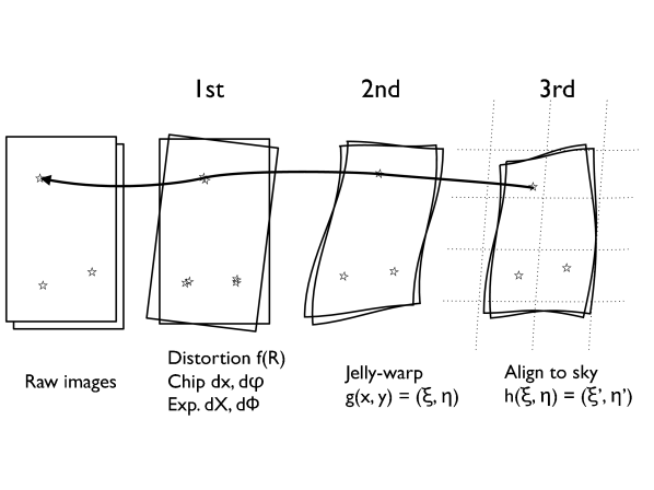
Figure 1.— Schematic of the three steps in the mosaic warp

Table 2Summary of the warp rules

	New	Original	Typical	Registration
Distortion f(R)	yes	yes	yes	$\sim 0.5$ pixel
Jelly-warp	yes	yes	no	$\sim 0.05$ pixel
Align to sky	yes	no	no	$\sim 0.05$ pixel
Astrometry	$\sim 0.2$ arcsec	uncontrolled	depending on pipelines

Once we have all of the parameters that describe these three steps, we carry out the image warp all at once rather than applying the transformation step by step. This integration of the procedures is necessary to minimize the artifacts due to the interpolation of pixels. We estimate pixel values via 3rd order bi-polynomial interpolation of $4\times 4$ source pixels. We employ the arithmetic mean for stacking.

3. Galaxy Catalog

To construct the galaxy catalog from the mosaic image, we use the imcat tools “hfindpeaks” (object detection) and “apphot” (photometry). We use the half-light radius “$r_{h}$” as the size of an object. Using this size, we can distinguish galaxies from stars by requiring that $r_{h}$ for galaxies satisfy the relation:

$$r_{h}>r_{h}^{*}+\sigma_{r_{h}^{*}},$$ (4)

where $r_{h}^{*}$ and $\sigma_{r_{h}^{*}}$ are the half-light radius of a a stellar image and its rms, respectively.

We merge our catalog of stars with the SDSS star catalog to calibrate the photometric zeropoint (see. Equations 5). Typically, the number density of stars to the depth of SDSS is several arcmin^-2; the precision of the astrometric catalog is $\lesssim 1^{\prime\prime}$.

We determine the photometric zeropoints for each subfield from the the SDSS photometric catalog following Utsumi et al. (2010). The transformation equation between the photometric systems is:

$$Rc_{Subaru}-r^{\prime}_{SDSS} = -0.314(r^{\prime}_{SDSS}-i^{\prime}_{SDSS})-0.011\quad{\rm for}\quad r^{\prime}_{SDSS}-i^{\prime}_{SDSS}<0.5$$

$$i^{\prime}_{Subaru}-i^{\prime}_{SDSS} = 0.102(i^{\prime}_{SDSS}-r^{\prime}_{SDSS})+0.002\quad{\rm for}\quad-0.5<i^{\prime}_{SDSS}-r^{\prime}_{SDSS}$$ (5)

To assess the depth of our images, we follow the standard procedure of SDFRED to derive the limiting magnitude (Yagi et al., 2002; Ouchi et al., 2004). We give the $5\sigma$ limiting magnitude in a 2^′′ photometric aperture in Table 1.

To remove low signal-to-noise regions around sufficiently bright stars, we need a procedure for constructing masks. Stars brighter than 20 th magnitude are usually saturated in a Suprime-Cam typical exposure with $\sim 100$ sec integration. We measure the actual PSF of Suprime-Cam over a wide dynamic range by compiling the PSF of faint and bright stellar objects. We divide the stellar samples into subsamples segregated by R-band magnitude, faint (20-20.5 magnitude), intermediate (18-18.5 magnitude) and bright (13.75-14.25 magnitude), combine them by taking the arithmetic mean, and then measure their radial profile. Although we take a mean profile of bright stars, we also reject exceedingly bright pixels by choosing an appropriate threshold for each images in order to avoid saturated areas or blooming regions.

For stars with R $<14$, there are not enough stars to determine the mean PSF. Thus we consider an optical model of Suprime-Cam to determine the size of the surrounding halo. The halo surrounding a bright star is a reflection from optical glass components in front of the CCDs. The nearest and second nearest optical elements close to the CCDs consist of the entrance window to the dewar and the filter; their distances from the CCDs are 10.0mm and 34.5mm, respectively. For both elements, the thickness and effective reflection index is 15.0mm and 1.460280, respectively. The focal ratio Suprime-Cam is 1.86. Thus light reflected on the first surface, the backside of the dewar window, should be located 71.3 arcsec away from original position. Light from the other surfaces appears 144 , 212, 284 arcsec away from the original position. This model is consistent with the data and we use it to derive the mask radii. Adopted mask radii for brighter stars are shown in Appendix 7.

We mask some stars with $R<11$ by visual inspection to remove obvious artifacts. Appendix 8 and 9 show the masks.

4. Basic Weak Lensing Analysis

To construct an initial weak lensing map we follow the procedures described in Miyazaki et al. (2002a, 2007) and Kurtz et al. (2012). In this section we review the selection of sources and the construction of the mass, noise, and B-mode maps. In discussing the B-mode map, we motivate the investigation (Section 5) of sources of systematic error in this map.

4.1. Sources

We use $23<m<26$ galaxies with detection significance $\nu>10$ as source galaxies. We eliminate high ellipticity objects with $|e|>0.6$ because these objects are sometimes blended. This magnitude range gives an average magnitude of 24.5 for the sources in both the GTO and DLS fields. The average source density is $34.5{\rm~{}arcmin}^{-2}$ and $31.6{\rm~{}arcmin}^{-2}$ for the GTO and DLS fields, respectively. Figure 2 shows number density maps of sources galaxies for weak lensing analysis.

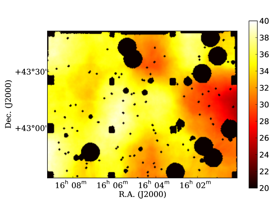
Figure 2.— Surface number density of weak lensing sources. For The GTO field (left) the sources have $23<R_{c}<26$; for the DLS field (right) the sources are in the range $23<i^{\prime}<26$.

Because we do not have measured redshifts for the source galaxies, we use the fitting formula from Schrabback et al. (2010) for galaxy redshifts as a function of magnitude in the range $23<i_{814}<25$. With this relation we estimate an average redshift of 1.2 for the DLS field where we have $i$-band data. For the GTO field where we have only $R$-band date, there is no suitable redshift-magnitude relation. We thus assume the same average redshift as the DLS field. If the actual redshift is 1.0 rather than assumed 1.2, we introduce an $\sim 10$% error in the estimate of the distance ratio. We note that this error in mass estimation is only important for absolute calibration.

To derive the ellipticities of the sources, we use getshapes, efit, and ecorrect in imcat. We evaluate the re-circularization correction using stars in the field of view and we model the PSF distortion as a fifth order bi-polynomial as a function of position. The $P_{\gamma}$ correction follows KSB+ (Hoekstra et al., 1998) who adopt a galaxy size dependent correction. The actual $\gamma$-field is discretized and noisy because it can only be estimated at the positions of galaxies. Note that we do not weight the estimated shear value according to galaxy’s magnitude. We apply a gaussian smoothing filter on the $\gamma$ field following Oguri & Hamana (2011). At first, we adopt a smoothing length, $\theta_{\rm G}=1.5^{\prime}$, following Kurtz et al. (2012).

4.2. Constructing the $\kappa$-S/N Map

We can now construct the $\kappa$-S/N map to search for mass concentrations based on the significance of the lensing signal. We derive the $\kappa$ map directly from the $\gamma$ map of the sources in Section 4.1. We divide this map by the noise map to obtain the $\kappa$-S/N map.

We use Monte Carlo realizations to construct the noise maps. We rotate the orientation of each source galaxy by a random angle. The randomized catalog is then the basis for the noise map. We repeat the Monte Carlo process 100 times, and then calculate the rms at each grid point of the noise map to estimate the noise at that point. The $\kappa$-S/N map then reflects the noise from intrinsic ellipticity noise and from variation in the number of galaxies.

In the following sections (Section 4.3, 4.4), we examine the systematic error in our weak lensing map by looking at the S/N distribution of the noise and B-mode maps. We demonstrate that the noise map obeys the expected Gaussian S/N distribution; however, the original B-mode map does not.

4.3. Testing the Noise Map

In the absence of signal, the S/N distribution for the noise map should match a standard normal distribution which has no free parameters. We test this expectation by constructing a “Noise S/N map” for each of the 100 Monte Carlo realizations. Pixel values on each of these map are strongly correlated spatially because the maps are smoothed with the Gaussian kernel. However a series of pixel values at a fixed position in the 100 “Noise S/N maps” should obey a normal distribution.

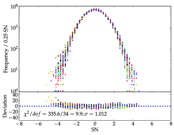
Figure 3.— [Top] S/N distributions for 100 noise maps in the GTO field, which are obtained by randomizing orientations of source galaxies. Different points indicate different realizations. The dashed line shows the expected normal distribution. [Bottom] panel shows the deviation from the normal distribution (Equation 6). The sum of these deviations divided by the degree-of-freedom is a measure of the systematic error.

We show the S/N histogram for randomized realizations in Figure 3. The random realizations have some scatter that we use to evaluate the presence of systematic errors in the B-mode map. To quantify the scatter, we define the “Deviation”:

$${\rm Deviation}=\frac{N_{i}^{\rm obs}-N_{i}^{\rm norm}}{\sqrt{N_{i}^{\rm norm}}}$$ (6)

where $N_{i}=dN/d(S/N)_{i}$ is a number of pixels per $d(S/N)_{i}$ bin in the observed (obs) and in the standard normal distribution (norm). The error is the standard deviation. We obtain the merit function as a kind of reduced chi-squared, $\tilde{\chi}^{2}$, from a sum of the squared deviations dividing by the the number degree of freedom (the number of bins):

$$\tilde{\chi}^{2}=\frac{1}{N-1}\sum_{i=0}^{N-1}\left(\rm{Deviation}\right)^{2}$$ (7)

Figure 4 shows the normalized cumulative distribution of $\tilde{\chi}^{2}$ for all random realizations. This wide range, $0\leq\tilde{\chi}^{2}\lesssim 65$, gives the maximum allowable difference between the noise and B-mode maps.

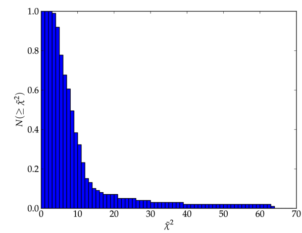
Figure 4.— Normalized cumulative distribution of the merit function $\tilde{\chi}^{2}$ (Equation 7) from the 100 realizations of the noise maps.

4.4. Testing the B-mode Map

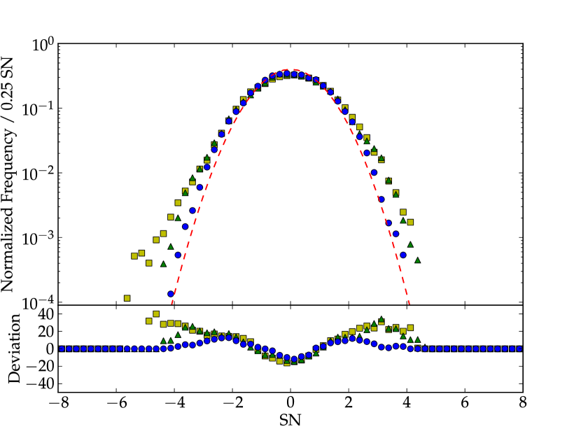
Figure 5.— [Top] Histogram of S/N values for B-mode maps derived from the new result (circles) as well as original (triangles) and typical (squares) stacking. The dashed line shows the expected normal distribution if there is no systematic error. [Bottom] Same as 3 but for the three kinds of B-mode.

In this section, we quantify the quality of the B-mode map. The standard B-mode map results from rotating each shear $|\gamma|\exp(2i\theta)$ by $\pi/4$, i.e. $\gamma_{1}+i\gamma_{2}\rightarrow-\gamma_{2}+i\gamma_{1}$, where $\theta$ is the position angle for each source. Because weak lensing does not produce a B-mode, we can evaluate the level of systematic error inherent in the mass reconstruction procedure by comparing the B-mode map with the noise map (Schneider et al., 2002).

Figure 5 shows the pixel distribution for the B-mode maps with the original, typical, and new stacking (Table 2). The S/N distribution has a large deviation relative to the standard normal distribution. The $\tilde{\chi}^{2}$ = 257 (1204) for the original (typical) stacking.

A possible origin of these B-mode artifacts is misalignment during the stacking procedure. Assuming we are stacking circular gaussian objects, a 10% positional inaccuracy generates $\sim 1$% artificial ellipticities. The positional difference applies to individual galaxies and their neighbors. The smoothing procedure then leads to detection of these $\sim 1$% ellipticities as a lensing signal. Thus stars must be registered internally with an accuracy of 1% level ($\sim$0.05 pixel).

Next we test procedures for reducing this kind of artificial signal in the B-mode map: (1) SkyFrame, (2) Wide FFTBox (3) Masking the edge of the field, (4) Higher order PSF anisotropy correction and (5) Smoothing cut off.

5. Reducing the B-mode Signal

Systemic issues which might produce an artificial signal in the B-mode map include errors in the physical coordinate system, excess large-scale power, boundary effects, and errors in the PSF anisotropy correction.

SkyFrame

If the stacked image is bent with respect to the physical coordinate system, the E-mode signal contaminates the B-mode. The tilt of the coordinates introduces a rotation of the sources.

The “new stacking” (Section 2.3) eliminates this bending. The “new stacking” image is aligned relative to the sky coordinate within $\sim 1$ pixel; the internal registration accuracy is $\sim 0.05$ pixel.

Wide FFTbox

There are two ways to perform the KSB analysis; (1) convolve the shear field with the complex kernel or (2) perform the convolution in the Fourier domain. Mathematically these procedures are identical. However, in practice for operation in the Fourier domain, boundary effects can be a problem. To avoid boundary effects present in the original reduction (Kurtz et al., 2012), we embedded the shear signal for the E/B-mode maps within a calculation box twice the size of the field with zero padding outside the map area.

Masking the edge of the field

At distances more than 15^′ from the optical axis the field of view of Suprime-Cam is vignetted (Miyazaki et al., 2002b). The distortion is also large, $\gtrsim 10^{\prime\prime}$, at the edge of the field. We thus try masking the region outside 15^′.

Smoothing cut off

To examine the origin of the remaining B-mode signal, we examine the power spectrum of the B-mode.

There is a significant excess in the power spectrum of the B-mode map relative to the noise map on large scales ($\gtrsim 10^{\prime}$). This excess is comparable with the power in the E-mode (Figure 6). The origin of this signal in the B-mode is unclear, but it should not be present.

To suppress this large scale systematic error in the B-mode map, we truncate the smoothing kernel at a scale of 10^′. Figure 5 shows the result. The truncation reduces the B-mode signal.

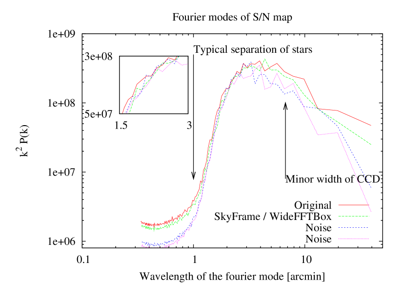
Figure 6.— Power spectrum of the noise maps (short dashed and dotted lines) and B-mode maps constructed with various procedures (all other curves as noted in the figure). The power spectrum for the B-mode has an excess relative to the noise maps on smaller scale less than the typical separation of stars and on scales larger than 10 ^′. For scales smaller than 1.5 ^′, smoothing decreases the amplitude of the power spectrum. The inset shows the power spectrum in the range 1.5 to 3 ^′. The SkyFrame procedure minimizes the excess in this range. A higher order PSF correction has no impact. For scales of 1 – 10 ^′, there is no significant excess of in the B-mode power spectrum. For scales larger than 10^′, all procedures fail to reduce the B-mode excess. Because the typical scale of a cluster of galaxies is few arcminutes, these scale can safely be filtered out.

Higher Order PSF anisotropy correction

To correct the PSF anisotropy induced by atmospheric disturbance or optical aberration, we applied a fifth order polynomial PSF model as a function of position. If the order of the polynomial is not sufficient to remove the systematic variations in the PSF, a B-mode is produced. To investigate this issue, we test a sixth-order polynomial.

5.1. Summary of the Tests

Table 3Summary of the Tests

Tests	$\tilde{\chi}^{2}$
Typical stacking image	1204.7
Original result	257.7
SkyFame	90.7
SkyFrame+Wide FFTBox	81.9
SkyFrame+Wide FFTBox+6th	84.3
SkyFrame+Wide FFTBox+Masking the edge	86.3
SkyFrame+Direct Convolution+Smoothing cut off	54.4

Table LABEL:tab:summarytests shows the result of these procedures. The “SkyFrame” registration reduces the B-mode power on small scales and the “Smoothing Cut-off” reduces the power on large scales (Figure 6). These two procedures have the largest effect on reduction of systematics in the B-mode map.

The “WideFFTBox” also reduces the B-mode but not significantly. We thus use direct convolution instead of the FFT implementation.

“Masking the edge of the field” and “Higher order PSF anisotropy correction” have little effect for the GTO field. “Masking the edge of the field” does not suppress systematics in the B-mode map. The same is true of the higher order corrections for PSF anisotropy.

Based on these results, we include

• SkyFrame image

• Smoothing Cut-off at 10 arcmin

• Direct convolution instead of using Wide FFT Box

in the construction of the maps. We show the result of this procedure in Figure 5. The pixel distribution of the B-mode S/N map indicates that residual systematics are reduced to a reasonably low level if we adopt appropriate procedures.

To assess whether the deviation of the B-mode signal is consistent with random realizations, we compare $\tilde{\chi}^{2}$ values with the distribution for each random realization. The maximum $\tilde{\chi}^{2}$ is larger than what we derive from the B-mode signal for the GTO field (Figure 4), $\tilde{\chi}^{2}=54.4$, much less than the original 257. Thus we confirm that the our revised lensing map is substantially less affected by systematic error. Figure 7 shows the resulting mass map with the “new warp” and Figure 8 shows the resulting S/N distribution for the both mass and B-mode map.

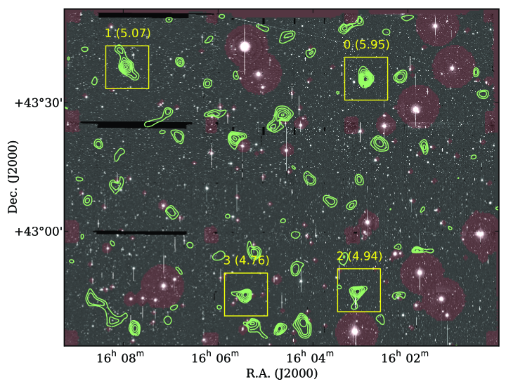
Figure 7.— Mass maps for the GTO field overlaid on Subaru images. Contours are drawn from $2\sigma$ threshold with an interval of $0.5\sigma$. Boxes show identified peak positions along with peak number and its significance. Masked region for brighter stars are also overlaid.

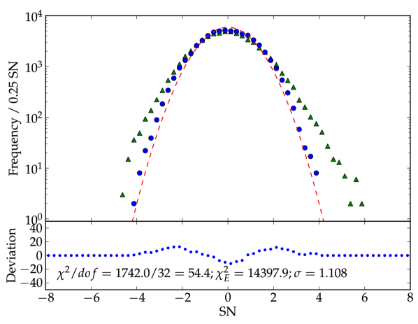
Figure 8.— S/N distributions for E-mode (triangles) and B-mode (circles) maps for the GTO fields. Lower panel shows the deviation from the normal distribution for the B-mode map.

5.2. The Impact of SkyFrame

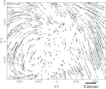
(a) GTO_0

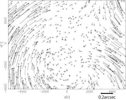
(b) GTO_1

Figure 9.— Displacement vector map of stellar positional differences between the undistorted detector coordinate (Section 2.3) and the stereographic projection of the celestial coordinate from the USNOA-2.0 catalog at the tangent point for the GTO subfield. The box shows approximately $32^{\prime}\times 27^{\prime}$ which is the field of view of Suprime-Cam. The length of the arrows indicate the positional difference in the detector coordinate multiplied by 1000. The displacement is complex and includes rotational components at the level of the pixel scale.

The most efficient procedure for reducing the B-mode systematics is “SkyFrame”. Figure 9 shows the displacement vector of positional difference for stars between the distortion free coordinate on the original warp and the stereographic projection of the celestial coordinate from the USNOA2.0 catalog at the tangent point. Although the displacement is small, a few pixels, there is a coherent pattern. Smoothing during construction of the map can introduce coherent patterns that dominate the noise from random ellipticities. These patterns can introduce the small scale B-mode signal. It is also possible to generate false E-mode signal from this coherent pattern.

There are two possible explanations for the residual pattern in the original warp: (1) an anisotropic distortion resulting from optical aberration, and/or (2) a disturbance in the curvature of the wave front due to atmospheric effects. The globally rotated component results from a small rotation of the image rotator. Higher order patterns vary from the field-to-field.

Yoshino et al. (2007) evaluated the anisotropy in the distortion from the corrector lens in Suprime-Cam with a positional accuracy of 0.4^′′. They found that there is an $\sim$0.8^′′ difference in the isotropic distortion pattern between the right and left edges of the field-of-view. These distortions are comparable with the residual of the displacement from the distortion free coordinate on the original image to the projected celestial coordinate.

These patterns are different for different observed fields (Figure 9(a) and Figure 9(b)). The difference between fields is the same as the difference of exposure-to-exposure because all frames are simply registered to the first frame in the series of exposures. These issues can be the source of the patterns we find.

A non-static factor like an atmospheric disturbance cannot explain the patterns. de Vries et al. (2007) show that longer exposures yield progressively lower ellipticities of the PSF (as $1/\sqrt{t_{\rm exp}}$ ) suggesting that the coherent differences shown in Figure 9(a) should not be caused from atmospheric disturbance.

6. Defining the Weak Lensing Peaks

At least two issues are important in defining the weak lensing peaks in the $\kappa$-S/N map. The smoothing length is important because it reduces the shape noise. Furthermore, the smoothing in part determines the sensitivity to cluster detection as a function of mass and redshift. The threshold for peak finding is also important. The fraction of false positives is sensitive to the threshold. Here we discuss these two issues.

6.1. Smoothing Length

In the previous sections, we constructed weak lensing mass maps with a fixed smoothing length of 1.5 ^′. A smaller smoothing length introduces more noise in the map resulting from shape noise. A larger smoothing length (larger than a few arcminutes) smooths out the cluster signal; the angular diameter of typical clusters for redshifts $0.2<z<0.7$, the range of sensitivity of the weak lensing maps, is several arcminutes.

Previous studies adopt a range of smoothing lengths. (Wittman et al., 2001; Miyazaki et al., 2002a; Hetterscheidt et al., 2005; Wittman et al., 2006; Schirmer et al., 2007; Gavazzi & Soucail, 2007; Miyazaki et al., 2007; Maturi et al., 2007; Bergé et al., 2008; Dietrich et al., 2007). To examine the effect of the smoothing length, we construct E/B-mode maps and random maps with three different smoothing lengths: $\theta_{\rm G}$ = 0.5^′, 1.0^′, and 1.5 ^′.

Figure 10 shows the relation between $\tilde{\chi}^{2}$ and $\theta_{\rm G}$. The $\tilde{\chi}^{2}$ of the E-mode increases with the smoothing length. The $\tilde{\chi}^{2}$ of the B-mode also increases.

The averaged $\tilde{\chi}^{2}$ value among 100 random realizations is $\tilde{\chi}^{2}>1$ and it increases with the square root of the smoothing length $\theta_{\rm G}$. This result occurs because the smoothing reduces the effective number of independent pixels. For small $\theta_{\rm G}$ the behavior of $\tilde{\chi}^{2}$ comes from the pixelization caused by dividing the smoothing kernel into coarse pixels. The shortest smoothing length, $\theta_{\rm G}=0.5^{\prime}$, corresponds to only $\approx 1.5$ pixels. The coarse sampling cannot reproduce the gaussian smoothing kernel well; thus the amplitude of the scaling relation may be changed and increased. This kind of pixelization effect is hard to describe analytically. Because the range, $0^{\prime}.5<\theta_{\rm G}<1^{\prime}.5$, might be affected by this pixelization effect, we do not correct for the number of effective pixels. We use the scale dependent $\tilde{\chi}^{2}(\theta_{\rm G})$ as a measure of the $\tilde{\chi}^{2}$.

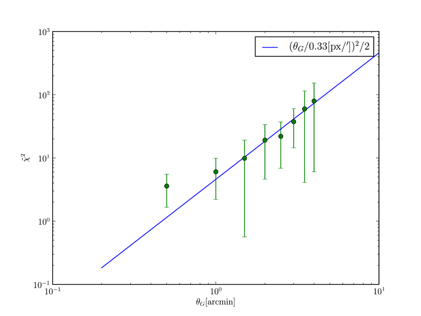
Figure 10.— Relation between the merit function $\tilde{\chi^{2}}$, and the smoothing scale $\theta_{\rm G}$. Points with errors denote mean values of $\tilde{\chi^{2}}$ and its standard deviation. The solid line shows $(\theta_{\rm G}/0.33[{\rm px}/^{\prime}])^{2}/2$, the square of the sigma of the Gaussian smoothing kernel in pixel units.

We estimate the optimal smoothing length for detecting clusters as a function of mass and redshift. Following Hamana et al. (2004), we analytically evaluate the expected S/N for weak lensing halos with universal NFW profiles. Because more distant clusters have smaller angular diameter, the S/N is redshift dependent. Furthermore, the typical scale radius of an NFW cluster depends on its mass; thus the S/N is also mass dependent. We compute the S/N as a function of smoothing scale $\theta_{\rm G}$. The S/N for less massive clusters ($M_{14}\equiv 10^{14}h^{-1}M_{\odot}$; $M_{14}=3.0$ for $z=0.5$, $M_{14}=1.0$ for $z=0.2$) reaches a maximum at $\theta_{\rm G}\approx 1.0^{\prime}$; more massive clusters are detected at greater S/N with a smoothing length larger than $\theta_{\rm G}\approx 1.0^{\prime}$. However, difference between 1.0^′ and 1.5 ^′ is small. At a fixed cluster mass, smaller smoothing lengths yield higher S/N at larger redshift. Because these effects are small, we choose $\theta_{G}=1.5^{\prime}$ .

6.2. Peak Definitions and Thresholds

We use SExtractor to locate peaks in the E-mode map; we require at least 3 connected pixels ($>2\sigma$) to define a peak. Selecting the appropriate threshold for a clean peak catalog is s subtle issue. Figure 11 shows the cumulative histogram of the highest peaks found in each noise map as a function of S/N. This figure shows the likelihood that significant peaks can be found accidentally. Statistics describing the highest peak for the 100 realizations are shown in the figure and summarized in Table 2.

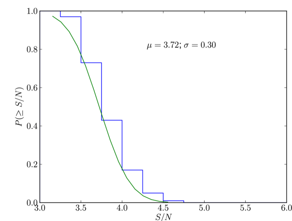
Figure 11.— Cumulative distribution of the highest peak S/N values for 100 realizations of noise maps for the GTO field. The solid line shows the expectation from the normal distribution.

We compare the cumulative peak counts with the expected standard normal distribution (green line). Figure 11 shows that the highest peak statistics of the noise maps are not well described by the theoretical curve. In other words, the highest peak statistics do not obey the ideal random Gaussian field. Thus we must derive these statistical quantities from Monte-Carlo simulations.

This discrepancy between the noise maps and the ideal case is more significant for smaller smoothing lengths. Based on these tests, we select different thresholds for each smoothing length. We consider two kinds of threshold: the $3\sigma$ threshold and the 99% threshold. The $3\sigma$ threshold is derived by assuming the standard normal distribution for the highest peaks; the 99% threshold is derived from “the most extreme peaks” among the highest peaks in the entire set of 100 noise map. Because it is based on the real data, the 99% threshold is much more reliable than the $3\sigma$ threshold and we use it throughout.

We summarize the $3\sigma$ and 99% thresholds in Table 2. As expected these thresholds differ for smaller smoothing lengths, but they are similar for $\theta_{G}=1.5$.

The numbers of detected peaks for each threshold are listed as $N_{3\sigma},N_{99\%}$ in Table 2.

Table 4S/N and Peak Statistics as a Function of the Smoothing Length $\theta_{\rm G}$

	S/N values			Max Peak				Detected Peak
$\theta_{\rm G}$	$\tilde{\chi}^{2}_{B}$	$\tilde{\chi}^{2}_{E}$	$\sigma$	$\mu$	$\sigma$	$(S/N)_{3\sigma}$	$(S/N)_{99\%}$	$N_{\rm 3\sigma}$	$N_{\rm 99\%}$
0.5	1.94	29.9	1.01	4.07	0.25	4.82	5.05	2	0
1.0	15.1	175	1.05	3.83	0.22	4.48	4.64	4	4
1.5	54.4	545	1.11	3.72	0.30	4.62	4.57	4	4

Next we consider the peaks in the E-mode map. With the smallest smoothing, there are no peaks. The shape noise of intrinsic ellipticities raises the threshold. The situation is different for $\theta_{G}=1.0$ and 1.5 because the larger smoothing involves more sources. The lensing signal becomes more significant for larger smoothing lengths.

As a quantitative representation of the significance of the weak lensing signal, we evaluate $\tilde{\chi}^{2}_{E}/\tilde{\chi}^{2}_{B}$. For the B-mode, $\tilde{\chi}^{2}$ should be small because there should be no signal; for the E-mode, $\tilde{\chi}^{2}$ should be larger reflecting the lensing signal.

The actual values of $\tilde{\chi}^{2}_{E}/\tilde{\chi}^{2}_{B}$ for $\theta_{G}=1.0$ and 1.5 are 11.6 and 10.0 for the GTO field. These similar values imply there is no strong preference for smoothing lengths between 1.0 and 1.5 in our data.

7. The DLS kappa Map

The procedures of Sections 5.1 generally apply to both the GTO and DLS field maps. Here we discuss the few issues that are particular to the DLS map.

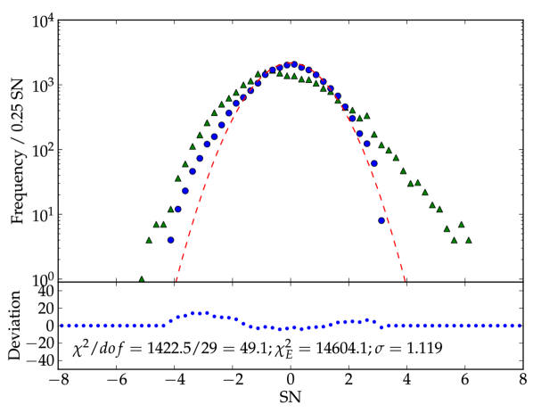
Figure 12.— Same as Figure 8 but for the DLS field.

For the DLS map, the $\tilde{\chi}^{2}$ for the original procedure is 134; for the new one it is 49.1 (Figure 12). The new value although reduced from the original one is not within the range for the random realizations (32 is the maximum value). The S/N distribution for the B-mode has a slight excess on the negative side.

We use $i^{\prime}$ band imaging in the DLS field rather than the $R_{C}$ band. We cannot determine the PSF anisotropy near the edge of the field because the star/galaxy separation is poor. Thus we trim objects located at the outer edge ($>15^{\prime}$ of the center of field). In contrast we do not trim the edges of the GTO field.

Even after this trimming, there is still a small excess in the S/N distribution for the B-mode on the negative side. However, the plus side seems to be well matched to the standard normal distribution. If we mask the three prominent negative excesses, the B-mode S/N distribution is in good agreement with the standard normal distribution. Thus the global correction may be sufficient and the residual local excess may be related to the most prominent peaks in the E-mode map. Figure 13 shows the $\kappa$-S/N map for the DLS field.

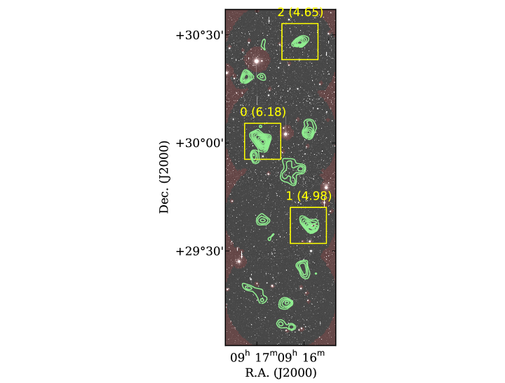
Figure 13.— Same as Figure 7 but for the DLS field.

Here we present the resulting $\kappa$-S/N maps for the DLS field (Figure 13)

8. Distribution of Peaks in Noise and B-Mode Maps

It is useful to have an analytical expression for the distribution of the highest peaks in order to test both the noise and B-mode maps. These expressions can then be used to estimate the fraction of false peaks in the $\kappa$-S/N maps.

We derive a probability density function that enables us to evaluate the probability of finding the highest peak in the noise map as a spurious peak in the $\kappa$-S/N map. We evaluate this probability as a function of the S/N. The probability density function that a random value $x$ obeying the normal distribution becomes the maximum value among $n$ samples is:

$$P_{n}(x)dx=\frac{n}{\sqrt{2\pi}}\exp\left(-\frac{x^{2}}{2}\right)\left(\frac{1}{2}{\rm erfc}\left(-\frac{x}{\sqrt{2}}\right)\right)^{n-1}dx$$ (8)

where ${\rm erfc}(x)$ is the complementary error function: ${\rm erfc}(x)=2/\sqrt{\pi}\int^{\infty}_{x}e^{-t^{2}}dt$. The first part of the product gives the probability of obtaining a random value of $x$, and the latter part describes the probability that the remaining $n-1$ random values are $<x$.

However, our map creation procedure is more complex because it applies gaussian smoothing which correlates pixel values spatially. We have to check the effect of the spatial correlation prior to evaluating the probability. We apply the smoothing function on the $\kappa$ map in the form $\exp\left(-(\theta/\theta_{\rm G})^{2}\right)$ where $\theta_{\rm G}/\sqrt{2}$ is the standard deviation of the smoothing kernel. Using the standard deviation as a measure of the correlation length, we reduce the total number of pixels in the mass map by a factor of $(\theta_{\rm G}/\sqrt{2})^{2}$. For example, in the GTO field where the total number of pixels is $300\times 234$ with a 0.33^′ / pixel scale, the effective number of pixels as a result of the smoothing becomes $300\times 234\times(0.33\times\sqrt{2}/\theta_{\rm G})^{2}$. After adopting $\theta_{\rm G}=1.5^{\prime}$, the effective number of pixels is 6,795.

Figure 14 shows both the analytic curve and the Monte Carlo results based on 10000 random realizations of the noise map. The analytic expression is an excellent representation of the Monte Carlo results.

In summary, Figure 14 shows that the smoothing procedure only reduces the number of independent pixels. Using this effective number in the probability function, we can evaluate the confidence level corresponding to a given S/N threshold. For example, a threshold of S/N = 4.66 corresponds to a 99.7% confidence level for the 2.12 deg² B-mode free massmap based on 1.5^′ smoothing. Similarly, S/N = 4.50 and 5.80 are the same 99.7% level confidence levels for a 1 and 1000 deg² degree survey, respectively.

Using this same formalism, we can derive an expression for the fraction of spurious peaks in the $\kappa$-S/N map above a given threshold. The probability of obtaining the $(m+1)$-th value in the descending set of ordered random values as a function of S/N is:

$$P_{n}^{(m)}(x)dx = \frac{(n-m){}_{n}C_{m}}{\sqrt{2\pi}}\exp\left(-\frac{x^{2}}{2}\right)\left(\frac{1}{2}{\rm erfc}\left(-\frac{x}{\sqrt{2}}\right)\right)^{n-m-1}\left(1-\frac{1}{2}{\rm erfc}\left(-\frac{x}{\sqrt{2}}\right)\right)^{m}dx$$ (9)

where ${}_{n}C_{m}=n!/(n-m)!m!$. With this general probability function, we can evaluate the expectation value for the number of peaks found in the noise field with a given S/N threshold:

$$N=\int_{(S/N){\rm th}}^{\infty}\sum_{m=0}^{n-1}P_{n}^{(m)}(x)dx$$ (10)

According to this formula, we should find on average 2.7 and 25.3 spurious peaks exceeding $(S/N)_{\rm th}=4.5$ and $4.0$, respectively, for a 1000 deg² survey with 1.5^′ Gaussian smoothing.

In conclusion, the analytical expression we derive is useful for future error analysis of large surveys. If we place a S/N $=4.5$ threshold on the B-mode-free kappa (S/N) map, we expect these high significant peaks to be uncontaminated at the 99.7% confidence level for a 1 deg² field; only 2.7 spurious peaks should be found on average for a 1000 deg² survey. Figure 15 shows the S/N threshold as a function of survey area.

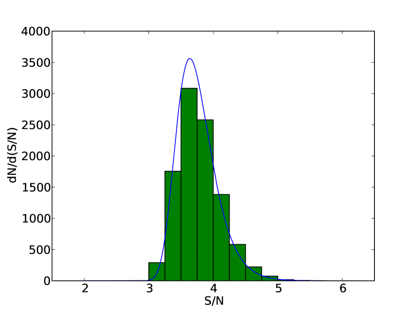
Figure 14.— S/N value distribution for maximum peaks among 10,000 noise map realizations for a field covering 2.12 deg² (histogram) and an analytical model (curve). The effective pixel number is the number of actual pixels divided by the smoothing length in pixel units.

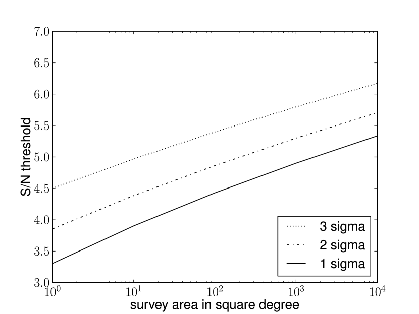
Figure 15.— S/N threshold dependence on survey area.

9. The Nature of the Weak Lensing Peaks

To test the reliability of the peak catalogs for the GTO (Figure 7) and DLS fields (Figure13), we next search for corresponding systems of galaxies. Weak lensing only traces the surface mass density. Thus our peaks may be single isolated clusters or superpositions of less massive groups along the line of sight. Here we test the peaks against dense foreground redshift surveys following Geller et al. (2005) and Kurtz et al. (2012).

9.1. Redshift Surveys

Dense redshift samples are available for both the GTO field (Kurtz et al., 2012) and the DLS field (Geller et al., 2005, 2010; Hwang et al., 2012). The redshift surveys were carried out with the Hectospec (Fabricant et al., 1998, 2005), a 300-fiber robotic instrument mounted on the MMT. The spectra cover the wavelength range 3,500-10,000Å with a resolution of $\sim 6$ Å. The typical error in an individual redshift (normalized by $(1+z)$) is 27 km/s for emission line objects and 37 km/s for absorption line objects. The surveys include redshifts for galaxies with $R\lesssim 20.6$ in the 4 deg² DLS field and redshifts for galaxies with $r_{\rm petro}<21.3$, $r-i>0.4$ and $g-r>1.0$ in the GTO 2deg² field. With these samples, we can identify massive clusters of galaxies with redshift $z\lesssim 0.6$. The surface number densities of the spectroscopic samples are 0.6 and 1.1 ${\rm arcmin}^{-2}$ for the GTO and the DLS fields, respectively.

To identify potential galaxy systems associated with the detected weak lensing peaks, we examine the redshift distributions in cones of 3^′ and 6^′ radius centered on the location of each of the weak lensing peaks.

We examine peaks in the redshift histograms. We define the significance of each peak as the difference between the number of galaxies $N$ and mean number of galaxies $\langle N\rangle$ expected in the cone at that redshift divided by the standard deviation $\sigma$: $(N-\langle N\rangle)/\sigma$. For neighbors satisfying $|\Delta z|<0.004(1+z)$, we calculate a velocity dispersion from the square root of the unbiased variance. We use the bootstrap to measure the error in the velocity dispersion.

Tables 5 and 6 list the weak lensing peaks for the GTO and DLS fields, respectively. The Tables list the lensing peak rank and significance, the celestial coordinates of the peaks, the rest frame velocity dispersion and its error, the number of peak members and its significance, and the mean redshift. The Table also include additional information from the literature.

(a) Redshift distribution for Peak GTO 00. The filled histogram shows objects within a cone of 3^′ radius centered on the weak lensing peak; the open histogram shows objects within a 6^′ cone. Bins in redshift are $0.002(1+z)$ wide.

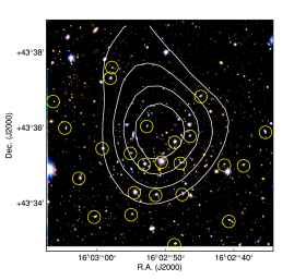
(b) Close-up view for Peak GTO 00. The image is 6${}^{\prime}\times 6^{\prime}$. Contours show the weak lensing peak. Small yellow circles identify galaxies in the redshift peak centered at a mean $z=0.416$.

Figure 16.— Peak GTO00

(a) Same as Figure 16(a) but for Peak GTO01.

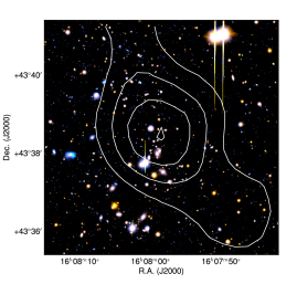
(b) Close up view for Peak GTO01.

Figure 17.— Peak GTO01

(a) Same as Figure 16(a) but for Peak GTO02.

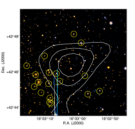
(b) Same as Figure 16(b). The mean redshift of the peak in Figure 18(a) corresponding to the weak lensing system is $z=0.540$

Figure 18.— Peak GTO02

(a) Same as Figure 16(a) but for Peak GTO03.

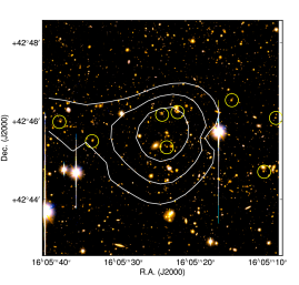
(b) Same as Figure 16(b). The significant peak in the redshift histogram (Figure 19(a)) corresponding to the lensing peak is $z=0.731$.

Figure 19.— Peak GTO03

(a) Same as Figure 16(a) but for Peak DLS00

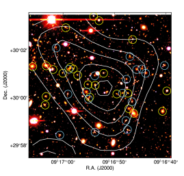
(b) Same as Figure 16(b). This weak lensing peak corresponds to a superposition of structures in the redshfit survey at redshifts $z=0.319$ (yellow circles) and $z=0.535$ (skyblue circles).

Figure 20.— Peak DLS00

(a) Same as Figure 16(a) but for Peak DLS01

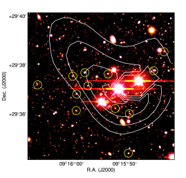
(b) Same as Figure 16(b). The mean redshfit of the peak in Figure 21(a) corresponding to the weak lensing system is $z=0.531$.

Figure 21.— Peak DLS01

(a) Same as Figure 16(a) but for Peak DLS02

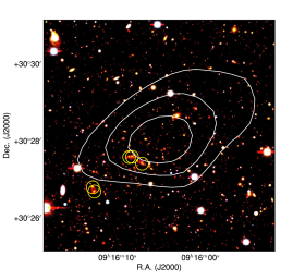
(b) Same as Figure 16(b). The mean redshfit of the peak in Figure 22(a) corresponding to the weak lensing system is $z=0.647$.

Figure 22.— Peak DLS02

9.2. The GTO Field

We list peaks in Table 5 that have S/N $\geq$ 3.7 as in Miyazaki et al. (2007). However, we concentrate on peaks with S/N$\geq$ 4.56 because our analysis of the noise maps shows that this higher threshold yields a more robust catalog.

The most significant peak, 0, has an obvious counterpart in the redshift histogram at a mean redshift $z=0.419$ (Figure 16(a)). Figure 16(b) shows the spatial distribution of cluster members within $\Delta z=0.004$ of the mean and within 3^′ of the weak lensing peak. It is clear that these galaxies are concentrated around the lensing peak. There is also extended x-ray emission associated with this system; the SDSS red sequence survey (Wen et al., 2009) also identifies it.

The lensing peak is slightly offset from the galaxy distribution. Assuming the brightest cluster member is the BCG, its offset is $\sim 1^{\prime}$, comparable with smoothing length.

Figure 17, corresponding to peak 1, shows a concentration of bright galaxies, but the redshift histogram does not show an obvious peak. This discrepancy may result from under-sampling at this location in the redshift survey (see peak 7 in Figure 2 of Kurtz et al. (2012)). Gunn et al. (1986) reported that this concentration of galaxies is a cluster with $z=0.2830$. The redshift histogram does show some galaxies around this redshift.

Peak 2 has a significance of 4.92 (Figure 18). This peak has a clear counterpart in the redshift histogram at a mean $z=0.540$. X-ray observations also show extended emission. Figure 18(b) shows the distribution of the suspected cluster members on the sky. The lensing peak is shifted by several arcminutes from the peak of galaxy distribution. The reason for the shift is not clear, but we suspect that because the peak is near the edge of the imaging field, there may be distortion in the $\kappa$-S/N map. This peak may also be affected by a neighboring bright star.

Peak 3 has a significance of 4.76 and, remarkably, corresponds to a peak in the redshift survey at $z=0.73$ (Figure 18). Although the spectroscopic sample is small, there is an excess in the galaxy count within 3^′ of the peak.

Above the S/N = 4.56 threshold, all of the peaks (with the possible exception of peak 1) correspond to systems of galaxies. We suspect that the failure to detect peak 1 in the redshift survey results from undersampling. The offsets in position between the lensing peaks and the lenses are consistent with the smoothing length except in a case where edge effects may be important.

Below the S/N = 4.56 threshold many fewer peaks correspond to systems of galaxies as we expect based on analysis of the noise maps. Table 5 lists possible systems associated with S/N$\geq 3.7$ peaks for comparison with previous work.

Table 5 Peak list for the GTO field.

Rank

$\nu$

RA2000

DEC2000

$\sigma_{p,6}$[km/s]

$N_{6}$

$z_{6}$

$\sigma_{p,3}$[km/s]

$N_{3}$

$z_{3}$

NED

X-ray

distance

0

5.95

16:02:50.826

+43:35:51.34

$992.0\pm 94.5$

$40(8.6\sigma)$

$0.415$(#1)

$1014.1\pm 113.2$

$24(11.8\sigma)$

$0.416$(#1)

$0.420$, XrayS

$9.10\pm 1.32$

1.156’

1

5.07

16:07:58.418

+43:38:23.99

$\bullet$

$\bullet$

$0.2830$

2

4.94

16:03:01.380

+42:46:32.00

$655.8\pm 94.8$

$29(12.0\sigma)$

$0.540$(#0)

$728.3\pm 127.7$

$18(13.9\sigma)$

$0.540$(#0)

$0.556$,$0.5391$,XrayS

$20.0\pm 1.5$

1.931’

3

4.76

16:05:24.866

+42:45:34.17

$497.9\pm 136.5$

$10(16.1\sigma)$

$0.731$

$562.8\pm 151.1$

$8(26.2\sigma)$

$0.731$

4

4.38

16:05:39.982

+43:22:13.70

5

4.29

16:04:37.615

+43:27:34.65

XrayS

6

4.19

16:04:41.282

+42:37:54.73

7

4.17

16:07:44.303

+42:37:45.58

8

4.12

16:04:10.464

+42:39:14.47

$411.9\pm 74.9$

$9(18.1\sigma)$

$0.673$(#3)

$508.6\pm 102.4$

$6(28.1\sigma)$

$0.673$(#3)

9

3.85

16:05:15.727

+42:39:14.39

10

3.70

16:01:46.456

+42:56:06.40

$421.9\pm 59.1$

$15(4.5\sigma)$

$0.256$

$366.1\pm 59.7$

$10(7.2\sigma)$

$0.287$

9.3. The DLS Field

In the DLS field (Figure 13), the most significant peak (0) has S/N = 6.18 (Figure 20). The redshift histogram (Figure 20(b)) shows two different concentrations centered at $z=0.320$ and $z=0.537$. This peak is apparently a superposition of clusters along the line of sight. So far, this peak is not covered by X-ray observations.

Peak 1 (Figure 21) has S/N = 4.98 but it unfortunately coincides with bright stars. The center of the weak lensing peak is masked by these bright stars. The redshift histogram shows a peak at $z=0.531$, but the velocity dispersion for the $3^{\prime}$ cone, $\sigma\sim 386$ km s^-1 is too low to account for the lensing peak: the 636 km s^-1 dispersion for the $6^{\prime}$ cone is sufficient to account for the detection. The coincident star compromises accurate measurement of the velocity dispersion.

Two other previous studies (lensing and X-ray) (Abate et al., 2009; Kubo et al., 2009) reported that there is a cluster at $z=0.53$. X-ray observations show extended emission suggesting that the velocity dispersion may be underestimated. The redshift distribution also shows a peak at at $z=0.183$ Thus the system at $z=0.53$ may be boosted by the foreground large-scale structure.

The third significant Peak 02 (Figure 22) has S/N = 4.56 and coincides with five galaxies around $z=0.65$ in the spectroscopic data (Figure 22(b)) even though such high $z$ galaxies are rare in the redshift survey. There is also extended x-ray emission associated with this peak.

In the DLS field, the results are less clear than in the GTO field. One of the peaks (2) is a cluster and one (0) is a clear superposition of clusters. The interpretation of peak 1 is unclear, but we believe the peak is not noise. In Table 6 we also list lower significance peaks and possibly associated systems of galaxies for comparison with previous work.

Table 6Peak list for the DLS field.

Rank

$\nu$

RA2000

DEC2000

$\sigma_{p,6}$[km/s]

$N_{6}$

$z_{6}$

$\sigma_{p,3}$[km/s]

$N_{3}$

$z_{3}$

NED

X-ray

distance

0

6.18

09:16:52.817

+30:00:28.44

$497\pm 50$

$47(7.8\sigma)$

$0.318$

$468\pm 61$

$23(9.3\sigma)$

$0.319$

$486\pm 75$

$25(7.0\sigma)$

$0.535$

$446\pm 79$

$18(13.7\sigma)$

$0.535$

1

4.98

09:15:54.449

+29:37:08.25

$636\pm 133$

$26(7.2\sigma)$

$0.531$

$386\pm 64$

$12(9.2\sigma)$

$0.531$

$0.53$

$4.99\pm 1.32(2.97)$

0.797’

2

4.65

09:16:04.967

+30:28:08.30

$524\pm 145$

$5(30.2\sigma)$

$0.647$

$524\pm 147$

$5(54.1\sigma)$

$0.647$

$9.52\pm 2.24(4.60)$

0.786’

$1.75\pm 1.21(0.65)$

1.677’

3

4.46

09:15:54.292

+30:03:08.24

4

4.24

09:17:12.960

+30:18:28.09

$811\pm 124$

$19(5.3\sigma)$

$0.535$

$859\pm 162$

$12(9.1\sigma)$

$0.535$

$29.1\pm 10.4(5.88)$

0.961’

5

3.86

09:16:20.559

+29:15:48.60

$1026\pm 188$

$13(11.2\sigma)$

$0.365$

$486\pm 187$

$8(17.7\sigma)$

$0.367$

$818\pm 99$

$25(7.0\sigma)$

$0.536$

$968\pm 169$

$12(9.1\sigma)$

$0.536$

10. Comparison with Earlier Results

The new maps of the GTO field and our 1 deg² portion of the DLS field contain seven weak lensing peaks above our threshold; these peaks are probably all associated either with a single system of galaxies or with a superposition along the line-of-sight. In other words, the analysis suggests that the lensing signal above our threshold is a reasonably robust measure of features of the large-scale structure of the universe.

Next we compare the results for the lensing peaks with previous work. The issues relevant for the GTO and DLS field are slightly different. In the GTO case, we analyze the same data as Kurtz et al. (2012), but we apply new procedures to reduce systematic error. In the DLS subfield, we apply essentially the same reduction procedure as the GTO field. Our Subaru DLS data are deeper and are taken in better conditions than the original data analyzed by Wittman et al. (2006).

For the GTO field, Kurtz et al. (2012) find two peaks with S/N $\geq 4.5$; we also find these peaks at S/N $\geq 4.56$ along with two additional ones. This difference occurs because the suppression of systematic errors changes the local peak values in the $\kappa$-S/N map. There is no change in the average sensitivity of the map.

The difference in the peak height distribution for the B-mode map of Kurtz et al. (2012) and our map demonstrates again that the systematic error suppression is effective. Kurtz et al. (2012) found 4 peaks with S/N$\geq 3.7$ in their B-mode map. We find only 2 peaks with this amplitude in our new B-mode map (S/N=3.90, 3.87). The highest B-mode peak now has S/N = 3.90 rather than 4.23.

Our data cover about 25% of the original DLS field F2. Wittman et al. (2006) identified one peak and Kubo et al. (2009) detected 3 peaks in this region of F2. All of these peaks have S/N$<3.9$, substantially below our revised threshold.

The original DLS F2 data were taken on the Kitt Peak 4-meter in the R-band image with PSF $<0.9^{\prime\prime}$; final co-added images reached a depth of $R\sim 26$ and the source galaxy density is, $\sim 20~{}{\rm arcmin}^{-2}$. The Subaru source density is $\sim 30~{}{\rm arcmin}^{-2}$ to roughly the same magnitude limit. The lower source galaxy density may result from the poorer seeing at Kitt Peak. In this case, the Subaru map is more sensitive mainly as a result of the increase source density. We find three peaks above the threshold S/N = 4.56; one of these is a cluster at $z=0.64$.

Obviously, at S/N below our revised threshold, there are peaks that correspond to systems of galaxies (Tables 5, 6). As we would expect, the fraction of “real” peaks declines with decreasing S/N.

11. Conclusion

Weak lensing is a powerful tool of modern cosmology. Its application to the detection of clusters of galaxies is limited to some extent by subtle systematic errors in the construction of the $\kappa$-S/N maps. Careful analysis of the B-mode maps where there should be no signal provides a route to reduction of these systematic errors. We use a set of noise maps along with the B-mode maps for two fields observed with the Subaru telescope to test procedures for the reduction of systematics.

Our tests of the B-mode maps against noise maps demonstrate that the following image processing procedures significantly reduce systematic error in the final $\kappa$-S/N map:

• Registration of positions onto the absolute celestial coordinate grid,

• Simultaneous application of all image transformations to avoid loss of information in interpolation, and

• Application of a smoothing cutoff at 10^′ to remove excess large-scale power.

By comparing the S/N distribution for noise and B-mode maps, we demonstrate that these revised procedures significantly reduce the systematics that otherwise appear in the B-mode map. We then take advantage of these revised procedures to show that weak lensing cluster detection is insensitive to the smoothing length for the $\kappa$-S/N map in the range $1.0^{\prime}$ to 1.5^′. Also on the basis of this analysis, we suggest use of the 99% threshold derived from the “most extreme peaks” among the highest peaks of the noise maps rather than the more standard 3$\sigma$ threshold. We provide an analytic expression for the distribution of these highest peaks that can be used to estimate the fraction of false peaks in the $\kappa$-S/N maps as a function of the detection threshold.

We test our systematic error reduction procedure and our high peak analysis by analyzing the GTO field and a portion of the DLS F2 field; together these fields cover $2.52{\rm deg}^{2}$. A threshold of 4.56 corresponds to the 99.5% confidence level from the highest peak analysis for our 1.5^′ smoothing length. We expect these peaks to be uncontaminated by false peaks over this total area. The data show seven peaks above this threshold; all of these peaks correspond to galaxy overdensities. Six of these peaks correspond to clusters of galaxies; one is a superposition of systems. Five of these peaks are well-sampled by dense foreground redshift surveys providing reliable estimates of the rest frame line-of-sight velocity dispersions of the clusters. One peak in the GTO field is in region sparsely sampled by the redshift survey, but a concentration of galaxies is evident in the imaging data. For one peak in the DLS field, foreground stars probably lead to an underestimate of the velocity dispersion from the spectroscopic data, but the peak is associated with extended x-ray emission. Taken together, these results substantiate the efficacy of our revised procedures.

The systematic error reduction procedures we apply are general and can be applied to future large-area weak lensing surveys. Our high peak analysis suggests that with a S/N threshold of 4.5, there should be only 2.7 spurious weak lensing peaks even in an area of 1000 deg² where we expect $\sim$ 2000 peaks based on our Subaru fields.

Appendix A Masks

Here we present details of masks described in Section 3. Table 7 shows the mask for brights stars based on the external catalog USNO-A2.0 (Monet, 1998). Table 8 and Table 9 show the coordinates for the additional manually constructed masks.

Table 7Masking Radius Around Bright Stars

Magnitude Range	Mask Radius (arcsec)
$R<9.0$	210
$9.0<R<10.0$	140
$10.0<R<12.0$	70
$12.0<R<14.0$	35
$14.0<R<16.0$	18
$16.0<R<18.0$	6

Table 8Manually Masked Regions around Bright Stars in the GTO Field.

RA2000	DEC2000	radius (arcsec)	Origin
240.11876	42.9889	270	Filter reflection
240.327	42.7408	270	Filter reflection
240.44033	42.842131	220	Filter reflection
240.45127	43.480879	270	Filter reflection
240.48183	43.629343	41.4	Incorrect position
240.77826	42.616311	270	Filter reflection
241.06437	43.414799	99	Dewar window reflection
241.16981	43.42311	36	Incorrect position
241.26726	43.561169	99	Dewar window reflection
241.3551	43.711462	270	Filter reflection

Table 9Manually Masked Regions Around Bright Stars in the DLS Field.

RA2000	DEC2000	radius (arcsec)	Origin
138.888195	29.792573	120	Dewar window reflection
139.343445	29.452575	120	Dewar window reflection
139.100387	30.040381	120	Dewar window reflection
139.254212	30.374562	120	Dewar window reflection
139.412442	30.320542	120	Dewar window reflection

References

- Abate et al. (2009) Abate, A., Wittman, D., Margoniner, V. E., Bridle, S. L., Gee, P., Tyson, J. A., & Dell’Antonio, I. P. 2009, ApJ, 702, 603
- Baba et al. (2002) Baba, H., Yasuda, N., Ichikawa, S.-I., Yagi, M., Iwamoto, N., Takata, T., Horaguchi, T., Taga, M., Watanabe, M., Ozawa, T., & Hamabe, M. 2002, in Astronomical Society of the Pacific Conference Series, Vol. 281, Astronomical Data Analysis Software and Systems XI, ed. D. A. Bohlender, D. Durand, & T. H. Handley, 298
- Bellagamba et al. (2011) Bellagamba, F., Maturi, M., Hamana, T., Meneghetti, M., Miyazaki, S., & Moscardini, L. 2011, MNRAS, 413, 1145
- Bergé et al. (2008) Bergé, J., Pacaud, F., Réfrégier, A., Massey, R., Pierre, M., Amara, A., Birkinshaw, M., Paulin-Henriksson, S., Smith, G. P., & Willis, J. 2008, MNRAS, 385, 695
- Bertin & Arnouts (1996) Bertin, E., & Arnouts, S. 1996, A&AS, 117, 393
- Dahle et al. (2003) Dahle, H., Pedersen, K., Lilje, P. B., Maddox, S. J., & Kaiser, N. 2003, ApJ, 591, 662
- de Vries et al. (2007) de Vries, W. H., Olivier, S. S., Asztalos, S. J., Rosenberg, L. J., & Baker, K. L. 2007, ApJ, 662, 744
- Dietrich et al. (2007) Dietrich, J. P., Erben, T., Lamer, G., Schneider, P., Schwope, A., Hartlap, J., & Maturi, M. 2007, A&A, 470, 821
- Fabricant et al. (2005) Fabricant, D., Fata, R., Roll, J., Hertz, E., Caldwell, N., Gauron, T., Geary, J., McLeod, B., Szentgyorgyi, A., Zajac, J., Kurtz, M., Barberis, J., Bergner, H., Brown, W., Conroy, M., Eng, R., Geller, M., Goddard, R., Honsa, M., Mueller, M., Mink, D., Ordway, M., Tokarz, S., Woods, D., Wyatt, W., Epps, H., & Dell’Antonio, I. 2005, PASP, 117, 1411
- Fabricant et al. (1998) Fabricant, D. G., Hertz, E. N., Szentgyorgyi, A. H., Fata, R. G., Roll, J. B., & Zajac, J. M. 1998, in Society of Photo-Optical Instrumentation Engineers (SPIE) Conference Series, Vol. 3355, Society of Photo-Optical Instrumentation Engineers (SPIE) Conference Series, ed. S. D’Odorico, 285–296
- Gavazzi & Soucail (2007) Gavazzi, R., & Soucail, G. 2007, A&A, 462, 459
- Geller et al. (2005) Geller, M. J., Dell’Antonio, I. P., Kurtz, M. J., Ramella, M., Fabricant, D. G., Caldwell, N., Tyson, J. A., & Wittman, D. 2005, ApJ, 635, L125
- Geller et al. (2010) Geller, M. J., Kurtz, M. J., Dell’Antonio, I. P., Ramella, M., & Fabricant, D. G. 2010, ApJ, 709, 832
- Gunn et al. (1986) Gunn, J. E., Hoessel, J. G., & Oke, J. B. 1986, ApJ, 306, 30
- Hamana et al. (2012) Hamana, T., Oguri, M., Shirasaki, M., & Sato, M. 2012, MNRAS, 425, 2287
- Hamana et al. (2004) Hamana, T., Takada, M., & Yoshida, N. 2004, MNRAS, 350, 893
- Hetterscheidt et al. (2005) Hetterscheidt, M., Erben, T., Schneider, P., Maoli, R., van Waerbeke, L., & Mellier, Y. 2005, A&A, 442, 43
- Hoekstra et al. (1998) Hoekstra, H., Franx, M., Kuijken, K., & Squires, G. 1998, ApJ, 504, 636
- Hwang et al. (2012) Hwang, H. S., Geller, M. J., Kurtz, M. J., Dell’Antonio, I. P., & Fabricant, D. G. 2012, ApJ, 758, 25
- Kaiser et al. (1995) Kaiser, N., Squires, G., & Broadhurst, T. 1995, ApJ, 449, 460
- Kaiser et al. (1998) Kaiser, N., Wilson, G., Luppino, G., Kofman, L., Gioia, I., Metzger, M., & Dahle, H. 1998, ArXiv Astrophysics e-prints
- Kocevski et al. (2009) Kocevski, D. D., Lubin, L. M., Gal, R., Lemaux, B. C., Fassnacht, C. D., & Squires, G. K. 2009, ApJ, 690, 295
- Kubo et al. (2009) Kubo, J. M., Khiabanian, H., Dell’Antonio, I. P., Wittman, D., & Tyson, J. A. 2009, ApJ, 702, 980
- Kurtz et al. (2012) Kurtz, M. J., Geller, M. J., Utsumi, Y., Miyazaki, S., Dell’Antonio, I. P., & Fabricant, D. G. 2012, ApJ, 750, 168
- Maturi et al. (2007) Maturi, M., Schirmer, M., Meneghetti, M., Bartelmann, M., & Moscardini, L. 2007, A&A, 462, 473
- Miyazaki et al. (2007) Miyazaki, S., Hamana, T., Ellis, R. S., Kashikawa, N., Massey, R. J., Taylor, J., & Refregier, A. 2007, ApJ, 669, 714
- Miyazaki et al. (2002a) Miyazaki, S., Hamana, T., Shimasaku, K., Furusawa, H., Doi, M., Hamabe, M., Imi, K., Kimura, M., Komiyama, Y., Nakata, F., Okada, N., Okamura, S., Ouchi, M., Sekiguchi, M., Yagi, M., & Yasuda, N. 2002a, ApJ, 580, L97
- Miyazaki et al. (2002b) Miyazaki, S., Komiyama, Y., Sekiguchi, M., Okamura, S., Doi, M., Furusawa, H., Hamabe, M., Imi, K., Kimura, M., Nakata, F., Okada, N., Ouchi, M., Shimasaku, K., Yagi, M., & Yasuda, N. 2002b, PASJ, 54, 833
- Monet (1998) Monet, D. G. 1998, in Bulletin of the American Astronomical Society, Vol. 30, American Astronomical Society Meeting Abstracts, 120.03
- Oguri & Hamana (2011) Oguri, M., & Hamana, T. 2011, MNRAS, 414, 1851
- Ouchi et al. (2004) Ouchi, M., Shimasaku, K., Okamura, S., Furusawa, H., Kashikawa, N., Ota, K., Doi, M., Hamabe, M., Kimura, M., Komiyama, Y., Miyazaki, M., Miyazaki, S., Nakata, F., Sekiguchi, M., Yagi, M., & Yasuda, N. 2004, ApJ, 611, 660
- Schirmer et al. (2007) Schirmer, M., Erben, T., Hetterscheidt, M., & Schneider, P. 2007, A&A, 462, 875
- Schirmer et al. (2003) Schirmer, M., Erben, T., Schneider, P., Pietrzynski, G., Gieren, W., Carpano, S., Micol, A., & Pierfederici, F. 2003, A&A, 407, 869
- Schneider et al. (2002) Schneider, P., van Waerbeke, L., & Mellier, Y. 2002, A&A, 389, 729
- Schrabback et al. (2010) Schrabback, T., Hartlap, J., Joachimi, B., Kilbinger, M., Simon, P., Benabed, K., Bradač, M., Eifler, T., Erben, T., Fassnacht, C. D., High, F. W., Hilbert, S., Hildebrandt, H., Hoekstra, H., Kuijken, K., Marshall, P. J., Mellier, Y., Morganson, E., Schneider, P., Semboloni, E., van Waerbeke, L., & Velander, M. 2010, A&A, 516, A63+
- Shan et al. (2012) Shan, H., Kneib, J.-P., Tao, C., Fan, Z., Jauzac, M., Limousin, M., Massey, R., Rhodes, J., Thanjavur, K., & McCracken, H. J. 2012, ApJ, 748, 56
- Utsumi et al. (2010) Utsumi, Y., Goto, T., Kashikawa, N., Miyazaki, S., Komiyama, Y., Furusawa, H., & Overzier, R. 2010, ApJ, 721, 1680
- Wen et al. (2009) Wen, Z. L., Han, J. L., & Liu, F. S. 2009, ApJS, 183, 197
- Wen et al. (2010) —. 2010, ApJS, 187, 272
- White et al. (2002) White, M., van Waerbeke, L., & Mackey, J. 2002, ApJ, 575, 640
- White et al. (2000) White, N. E., Giommi, P., & Angelini, L. 2000, VizieR Online Data Catalog, 9031, 0
- Wittman et al. (2006) Wittman, D., Dell’Antonio, I. P., Hughes, J. P., Margoniner, V. E., Tyson, J. A., Cohen, J. G., & Norman, D. 2006, ApJ, 643, 128
- Wittman et al. (2001) Wittman, D., Tyson, J. A., Margoniner, V. E., Cohen, J. G., & Dell’Antonio, I. P. 2001, ApJ, 557, L89
- Wittman et al. (2002) Wittman, D. M., Tyson, J. A., Dell’Antonio, I. P., Becker, A., Margoniner, V., Cohen, J. G., Norman, D., Loomba, D., Squires, G., Wilson, G., Stubbs, C. W., Hennawi, J., Spergel, D. N., Boeshaar, P., Clocchiatti, A., Hamuy, M., Bernstein, G., Gonzalez, A., Guhathakurta, P., Hu, W., Seljak, U., & Zaritsky, D. 2002, in Society of Photo-Optical Instrumentation Engineers (SPIE) Conference Series, Vol. 4836, Society of Photo-Optical Instrumentation Engineers (SPIE) Conference Series, ed. J. A. Tyson & S. Wolff, 73–82
- Xmm-Newton Survey Science Centre (2010) Xmm-Newton Survey Science Centre, C. 2010, VizieR Online Data Catalog, 9041, 0
- Yagi et al. (2002) Yagi, M., Kashikawa, N., Sekiguchi, M., Doi, M., Yasuda, N., Shimasaku, K., & Okamura, S. 2002, AJ, 123, 66
- Yoshino et al. (2007) Yoshino, A., Yamada, Y., Nakata, F., Enoki, M., Takata, T., & Ichikawa, S. 2007, Report of the National Astronomical Observertory of Japan, 10, 19