Time-resolved Analysis of Fermi GRBs with Fast and Slow-Cooled Synchrotron Photon Models

Abstract

Time-resolved spectroscopy is performed on eight bright, long gamma-ray bursts (GRBs) dominated by single emission pulses that were observed with the Fermi Gamma-ray Space Telescope. Fitting the prompt radiation of GRBs by empirical spectral forms such as the Band function leads to ambiguous conclusions about the physical model for the prompt radiation. Moreover, the Band function is often inadequate to fit the data. The GRB spectrum is therefore modeled with two emission components consisting of optically thin non-thermal synchrotron radiation from relativistic electrons and, when significant, thermal emission from a jet photosphere, which is represented by a blackbody spectrum. To produce an acceptable fit, the addition of a blackbody component is required in 5 out of the 8 cases. We also find that the low-energy spectral index $\alpha$ is consistent with a synchrotron component with $\alpha=-0.81\pm 0.1$. This value lies between the limiting values of $\alpha=-2/3$ and $\alpha=-3/2$ for electrons in the slow and fast-cooling regimes, respectively, suggesting ongoing acceleration at the emission site. The blackbody component can be more significant when using a physical synchrotron model instead of the Band function, illustrating that the Band function does not serve as a good proxy for a non-thermal synchrotron emission component. The temperature and characteristic emission-region size of the blackbody component are found to, respectively, decrease and increase as power laws with time during the prompt phase. In addition, we find that the blackbody and non-thermal components have separate temporal behaviors as far as their respective flux and spectral evolutions.

1. Introduction

The fireball model of GRBs (Cavallo & Rees, 1978; Goodman, 1986; Paczyński, 1986) assumes that a large amount of energy is released in a small space leading to a fireball that emits $\gamma$-rays. The progenitors of these events are not known, but are believed to be the collapse of massive stars, or the coalescence of two compact objects. Details of this model rely heavily on assumptions about the initial parameters of the fireball including the radii of emission, the baryon load and the magnetic field associated with the plasma outflow (for review see Mészáros (2006)). The observed spectra of GRBs are typically interpreted as non-thermal (Piran, 1999; Zhang et al., 2012) though there are some exceptions (Ryde, 2004). This interpretation indicates that a dissipative process such as internal shocks energizes the electrons to non-thermal distributions. Though some versions of the fireball model predict that the entire spectrum in the $\gamma$-ray band be in the form of thermal emission, we concentrate on the version presented in Mészáros & Rees (2000) where a mixture of thermal and non-thermal (synchrotron) emission emerges. Alternative models such as the Poynting-flux dominated outflow (PFD) model exist and could provide a viable mechanism for generating the observed prompt emission (e.g., Giannios, 2009; Zhang & Yan, 2011). These PFD models have not yet advanced to quantitative spectral and temporal predictions; therefore, it is difficult to compare our results to these models as extensively as is possible for the internal shock model for which extensive simulations of lightcurves and spectra have been developed (e..g., Daigne & Mochkovitch, 1998; Bos̆njak, Daigne, & Dubus, 2009). The physical emission process behind these extreme cosmic explosions has not been established. In the past, GRB spectra have been well fit by the Band function (Band et al., 1993), which is an exponentially cutoff power law that smoothly joins to a second power law, and is parameterized by the function

$$F_{\nu}(\mathcal{E})\;=\;F_{0}\begin{cases}{\left(\frac{\mathcal{E}}{\rm 100\;keV}\right)^{\alpha}{\rm exp}\left(-\frac{(2+\alpha)\mathcal{E}}{E_{\rm p}}\right),}&{\mathcal{E}\leq(\alpha-\beta)\frac{E_{\rm p}}{(\alpha+2)}}\\ {\left(\frac{\mathcal{E}}{\rm 100\;keV}\right)^{\beta}{\rm exp}{\left(\beta-\alpha\right)}\left[\frac{(\alpha-\beta)E_{\rm p}}{{\rm 100\;keV}(2+\alpha)}\right]^{\alpha-\beta}},&{\mathcal{E}>(\alpha-\beta)\frac{E_{\rm p}}{(\alpha+2)}\;,}\end{cases}$$ (1)

where $\mathcal{E}$ is the photon energy. The Band function is characterized by low and high-energy power-law spectral indices (the Band $\alpha$ and Band $\beta$ parameters, respectively) as well as its $\nu F_{\nu}$ peak energy, E_p. The ability of the Band function to fit most prompt-spectra has led to the widespread use of the Band function’s fitted parameters as indicators of the underlying emission and acceleration processes. In particular, the value of $\alpha$ has been of interest because non-thermal spectra and indices from synchrotron, inverse Compton, and other processes are each constrained by allowed indices at energies less than their respective $\nu F_{\nu}$ peaks. Above the peak, the high-energy index is variable and related to the distribution of the emitting electrons and provides fewer clues for discerning between emission processes. Although such extrapolations can be useful, Burgess et al. (2011) (hereafter B11) directly fit a synchrotron photon model to the prompt emission data of GRB 090820A, showing that it is possible to fit a physical model directly to the data without relying on interpretations of the Band function in order to determine the $\gamma$-ray emission process.

Previous studies (González et al., 2003; Ryde, 2005; Guiriec et al., 2010; Ryde et al., 2010; Guiriec et al., 2013) showed that a single Band function cannot fully account for the spectrum of all GRBs. The addition of a blackbody and/or power-law better describes the spectra of these GRBs. Specifically, the addition of the blackbody below E_p also allows for the direct fitting of the synchrotron model to the data, which we exploit in this work. The addition of a blackbody in the spectrum allows a quantitative analysis of its properties to ascertain its origin. Several studies (Mészáros & Rees, 2000; Daigne & Mochkovitch, 2002; Ryde, 2004; Ryde et al., 2006) have developed the theoretical framework for a blackbody component coexisting with a non-thermal component in the spectra of GRBs, as well as testable relations that can be applied to data to investigate the photosphere of GRBs.

Herein, we extend the analysis of B11 to several bright Fermi GRBs and in addition investigate the ability of the Band function to serve as a proxy for physical emissivities in the fitting process. We show that slow-cooled synchrotron is a viable model for GRB prompt emission using data from both the Gamma-ray Burst Monitor (GBM) (10 keV - 40 MeV) and Large Area Telescope (LAT) (100 MeV - 300 GeV) on board the Fermi space telescope. This analysis makes use of the newly released LAT low-energy (LLE) data which provides a larger effective area between 30 MeV and $\sim$1 GeV, allowing us to extend the LAT analysis down to 30 MeV (see Pelassa et al., 2010, and work in preparation). First, we give a description of the non-thermal and blackbody photon emissivities in Section 2. We then present our analysis technique in Section 3 and compare the results with predictions about each component in Section 4. We discuss the results in Section 5, and constraints on synchrotron shell models are presented in the Appendix.

2. Model Spectral Components

In the fireball model of GRBs, the majority of the flux is theoretically expected to be in the form of thermal emission coming from the photosphere of the jet. However, nearly all of the low-energy indices implied by GRB spectral analysis with Band-function spectral inputs have $\alpha<+1$, i.e. too soft to be thermal – see for example Goldstein et al. (2012a, b) for the BATSE database. This points to a non-thermal emission process for most GRBs. Multi-spectral component analysis of Fermi GRBs has shown that while the majority of the emission is non-thermal, a small fraction of the energy radiated apparently originates from a blackbody component (Guiriec et al., 2011; Axelsson et al., 2012). In B11, a blackbody component was also identified when the non-thermal emission was fit with a synchrotron photon model. This combination of blackbody and non-thermal emission was predicted by Mészáros & Rees (2000). In this paper, before proceeding to the details of the analysis, we first review the synchrotron model (see B11), and also several observable relations of the blackbody component. These components are then implemented into a fitting program which directly convolves the physical models with the GBM detector response to compare with observations.

2.1. Synchrotron Radiation

While no definitive model for the non-thermal emission of GRBs exists, electron synchrotron is the simplest and most efficient non-thermal emission process that could account for the prompt GRB radiation. It is a natural first choice in moving from the traditional use of empirical fitting functions to physical models, which will then afford more reliable tests for characterizing the GRB environment. In B11, we implemented a parameterized synchrotron model for fitting GRB data directly. We implemented a synchrotron model first used in fitting the deconvolved spectra of GRBs by Tavani (1996) and later by Baring & Braby (2004). Sari, Piran, & Narayan (1998) identified two regimes for the synchrotron emission which are relevant for GRBs: fast and slow-cooling. The difference between the two is related to the radiative time-scale of the emission.

For the slow-cooling synchrotron model, we assume the electron distribution from B11 (see also Baring & Braby (2004)) which includes electrons in a thermal pool as well as electrons that are accelerated into a power-law tail (see Figure 1), given by

$$n_{e}(\gamma)\;=\;n_{0}\biggl{[}\;\Bigl{(}\hbox{${{\displaystyle\gamma\vphantom{(}}\over{\displaystyle\gamma_{\hbox{\sixrm th}}\vphantom{(}}}$}\Bigr{)}^{2}\,e^{-\gamma/\gamma_{\hbox{\sixrm th}}}+\epsilon\,\Bigl{(}\hbox{${{\displaystyle\gamma\vphantom{(}}\over{\displaystyle\gamma_{\hbox{\sixrm th}}\vphantom{(}}}$}\Bigr{)}^{-\delta}\,\Theta\Bigl{(}\hbox{${{\displaystyle\gamma\vphantom{(}}\over{\displaystyle\gamma_{\hbox{\sixrm min}}\vphantom{(}}}$}\Bigr{)}\,\biggr{]}\,.$$ (2)

Here, $n_{0}$ normalizes the distribution to total number or energy, $\gamma$ is the electron Lorentz factor in the fluid frame, $\gamma_{\hbox{\sixrm th}}$ is the thermal electron Lorentz factor, $\gamma_{\hbox{\sixrm min}}$ is the minimum electron Lorentz factor of the power-law tail, $\epsilon$ is the normalization of the power-law, and $\delta$ is the electron spectral index. The function $\Theta(x)$ is a step function where $\Theta(x)=0$ for $x<1$ and $\Theta(x)=1$ for $x>1$. In analyses of the shock acceleration process, distributions like eq. (2) are realized for $\epsilon\ll 1$ regimes both for non-relativistic shocks (e.g., Baring, Ellison, & Jones, 1995), and also ones where the upstream flow impacts the shock layer relativistically (Ellison, Jones & Reynolds, 1990; Ellison & Double, 2004; Spitkovsky, 2008; Baring, 2011; Summerlin & Baring, 2012). In all these works, the charges (in this case electrons) are accelerated directly from the thermal pool to generate a power-law distribution corresponding to $\epsilon\mathrel{\mathchoice{\lower 2.0pt\vbox{\halign{$\m@th\displaystyle\hfil#\hfil$\cr<\crcr\sim\crcr}}}{\lower 2.0pt\vbox{\halign{$\m@th\textstyle\hfil#\hfil$\cr<\crcr\sim\crcr}}}{\lower 2.0pt\vbox{\halign{$\m@th\scriptstyle\hfil#\hfil$\cr<\crcr\sim\crcr}}}{\lower 2.0pt\vbox{\halign{$\m@th\scriptscriptstyle\hfil#\hfil$\cr<\crcr\sim\crcr}}}}0.1$ that smoothly connects to the thermal distribution. This is no surprise since strong dissipation is present in plasma shocks, and so thermalization is prominent for many (but not all) particles. These results motivate our general form for the electron distribution, noting that our parametrization may oversimplify the process of acceleration and ignores the effects of photon-electron collisions such as Compton scattering that are likely taking place in the high $\gamma$-ray regime. In particular, as pointed out by (Baring & Braby, 2004), the distribution in Eq. (2) is only viable for approximating GRB spectra with synchrotron emission when $\epsilon\gg 1$, and the power-law component dominates the Maxwell-Boltzmann one. This constraint is accommodated in our fitting protocol, and we discuss its value shortly.

Finally, note that simulations that include the full radiative heating and cooling of electrons expected in the high $\gamma$-ray regime but that neglect acceleration processes produce electron distributions that differ greatly from simple power-laws (Pe’er & Waxman, 2004). These complicated electron distributions are difficult to model in a fitting process and may require spectral resolution beyond what the Fermi data provide to identify in spectral fits.

We convolve this simplified distribution with the standard isotropic synchrotron kernel (Rybicki & Lightman, 1979)

$$F_{\nu}(\mathcal{E})\;\propto\;\int_{1}^{\infty}n_{e}(\gamma)\,\mathcal{F}\left(\hbox{${{\displaystyle\mathcal{E}\vphantom{(}}\over{\displaystyle\mathcal{E}_{c}\vphantom{(}}}$}\right)\,d\gamma\quad,$$ (3)

where

$$\mathcal{F}\left(w\right)\;=\;w\int_{w}^{\infty}K_{5/3}(x)\,dx$$ (4)

expresses the single-particle synchrotron emissivity (i.e., energy per unit time per unit volume) in dimensionless functional form. The $K_{5/3}$ term is the modified Bessel function of the second kind. The characteristic scale for the synchrotron photon energy is

$$\mathcal{E}_{c}\;=\;E_{*}\gamma^{2}\ ,$$ (5)

where $E_{*}\equiv 3\Gamma B/(2B_{cr})\,m_{e}c^{2}$, B is the magnetic field strength, $\Gamma$ is the bulk Lorentz factor, and $\,B_{\rm cr}=4.41\times 10^{13}\,$Gauss is the quantum critical field.

In principle, there are six spectral parameters that can be constrained by the fits: $n_{0}$, $E_{*}$, $\delta$, $\epsilon$, $\gamma_{\hbox{\sixrm th}}$, and $\gamma_{\hbox{\sixrm min}}$; however, we fix $\gamma_{\hbox{\sixrm th}}$, $\gamma_{\hbox{\sixrm min}}$, and $\epsilon$ due to fitting correlations as explained below. The parameter $E_{*}$ scales the energy of the fit and is linearly related to the Band function’s E_p. Numerical simulations of particle acceleration at relativistic shocks have shown (see references in Baring & Braby, 2004) that the non-thermal population is generated directly from the thermal one. To match these circumstances, we set the ratio of $\gamma_{\hbox{\sixrm th}}$ and $\gamma_{\hbox{\sixrm min}}$ to be $\sim$3, following (Baring & Braby, 2004). The parameters $E_{*}$, $\gamma_{\hbox{\sixrm th}}$, and $\gamma_{\hbox{\sixrm min}}$ all directly scale the peak energy of the spectrum but do not alter its shape and thus cannot be independently determined. For this reason we chose values of $\gamma_{\hbox{\sixrm th}}=300$ and $\gamma_{\hbox{\sixrm min}}=900$ for all fits and left $E_{*}$ free to be constrained from the fit.

As shown in the Appendix, such parameter values are on the outer edge for what is allowed energetically. For these parameters, the flow is strongly Poynting flux/magnetic-field energy dominated in order that electrons with $\gamma\sim 300$ – 900 can produce radiation in the MeV regime. Magnetized jet models are advantageous for energy dissipation through magnetic reconnection, to produce short timescale variability, and to accelerate ultra-high energy cosmic ray (see Appendix). In fact, a wide range of parameter values with much larger electron Lorentz factors and smaller magnetic fields are possible. In weak magnetic-field models, a strong self-Compton component and $\gamma\gamma$ opacity effects can make a cascade that modifies the standard emission spectrum of GRBs. By considering a strongly magnetically dominated model, these issues can be neglected.

For the chosen parameters, the system is always in the strongly cooled regime (see Appendix). Nevertheless, we adopt the expression, eq. (2), to approximate an electron spectrum in the slow-cooling regime. The parameter $\epsilon$, corresponding to the relative amplitude between the thermal and non-thermal portions of the electron distribution, was not easily constrained in the fitting process used in B11 and produced small non-physical discontinuities in the electron distribution, as pointed out in Beloborodov (2013). Therefore, here we numerically fix this parameter to the small value of $(\gamma_{\hbox{\sixrm min}}/\gamma_{\hbox{\sixrm th}})^{2}\times\exp(-\gamma_{\hbox{\sixrm min}}/\gamma_{\hbox{\sixrm th}})$, so that there is no discernible discontinuity between the thermal and non-thermal parts of the distribution. The thermal component helps smooth out the spectral structure at $E_{\ast}$, but does not alter the asymptotic index of $\alpha=2/3$ realized for synchrotron emission from populations with lower bounds to their particle energies. After these simplifications, three shape parameters remain free: $E_{*}$, $\delta$ and $n_{0}$, which corresponds to the amplitude. Compared with the Band function’s four fit parameters this model is simpler yet tied to actual physical processes.

The second regime of synchrotron emission is the so-called fast-cooling regime, which applies for the adopted parameters in a naive cooling model. We assume that some acceleration process injects a power-law distribution of electrons

$$N^{\rm inj}_{e}(\gamma)\;=\;n_{e}(\delta-1)\gamma_{\hbox{\sixrm min}}^{(\delta-1)}\gamma^{-\delta}\;,\;\gamma_{\hbox{\sixrm min}}\leq\gamma$$ (6)

into a region where they are allowed to cool. Here, $n_{e}$ is the electron density. We neglect the inclusion of the thermal pool because its association with the radiative region is poorly understood. Moreover, we show below that the fast-cooling spectrum is already too broad for the typical GRB $\nu F_{\nu}$ peak and the thermal distribution only broadens the spectrum further. Neglecting adiabatic losses and other acceleration mechanisms, the cooling of electrons is governed by the continuity equation (Blumenthal & Gould, 1970)

$$\frac{\partial n_{e}(\gamma,t)}{\partial t}+\frac{\partial}{\partial\gamma}[\dot{\gamma}n_{e}(\gamma,t)]+\frac{n_{e}(\gamma,t)}{t_{esc}}\;=\;N^{\rm inj}_{e}(\gamma)$$ (7)

where $n_{e}/t_{esc}$ represents the loss of particles from the emission region from which we can define the maximal cooling scale $\gamma/\dot{\gamma}\;\sim\;t_{esc}$. This corresponds to a Lorentz factor, $\gamma_{cool}$, below which cooling shuts off. We expect that $\gamma_{cool}$ lies well below $\gamma_{\hbox{\sixrm min}}$ owing to the fact that a cooling break has not been observed in GRB data (see, however, Ackermann et al., 2012b). For very high electron Lorentz factors, $\gamma/\dot{\gamma}\;\ll\;t_{esc}$ and therefore the loss term can be neglected, i.e., the dynamical timescale is much longer than the radiative timescale. With this assumption we can simplify eq. (7) and it becomes time independent. The resulting electron distribution can then easily be solved for

$$n_{e}(\gamma,t)\;\approx\;\frac{1}{\dot{\gamma}}\int_{\gamma}^{\infty}N^{\rm inj}_{e}(\gamma^{\prime})d\gamma^{\prime}.$$ (8)

Substituting in the synchrotron cooling rate

$$\dot{\gamma}\;=\;-\frac{4}{9}\frac{r_{0}c}{r_{g}^{2}}\gamma^{2}\;,$$ (9)

where $r_{g}\;=\;m_{e}c^{2}/eB$ and $r_{0}\;=\;e^{2}/m_{e}c^{2}$, eq. (8) yields the synchrotron-cooled broken power-law distribution of electrons (see Figure 2)

$$n_{e}^{cool}\;\propto\;\frac{n_{e}\gamma_{\hbox{\sixrm min}}}{\gamma^{2}}\;\min\left\{\left(\frac{\gamma}{\gamma_{\hbox{\sixrm min}}}\right)^{-(\delta-1)},1\right\}\;,\;\gamma_{cool}\leq\gamma.$$ (10)

This distribution is convolved with eq. (4) to produce a photon spectrum. The radiation spectrum generated by this distribution has an asymptotic low-energy index of $-$3/2, the so-called “second line-of-death” (Cohen et al., 1997). The free parameters used for fitting this spectrum are the electron spectral index, $\delta$, the fast-cooling equivalent of $E_{*}$ and the overall amplitude. However, the majority of GRB spectra in the BATSE (Goldstein et al., 2012b) and GBM (Goldstein et al., 2012a) spectral catalogs have spectra with low-energy indices harder than $-$3/2. Even if the spectra were consistent with the low-energy index, the fast-cooling spectrum’s curvature around the $\nu F_{\nu}$ peak is much broader than that observed around the peak of the spectrum (See 4.2).

Even though we examine a model with $\gamma_{th}=300$ and $\gamma_{min}=900$, the spectral fitting is insensitive to the exact value of the product $\Gamma B\gamma^{2}$ provided that the constraints discussed in Appendix A are satisfied. Even in a strong cooling regime defined by these low assumed values of $\gamma_{th}$ and $\gamma_{min}$, second-order processes in GRBs (Waxman, 1995; Dermer & Humi, 2001), which can become more important than first-order processes in relativistic shocks (Dermer & Menon, 2009), allow us to consider a model that is effectively slowly cooled. Simulations typically have more parameters than our current model (Pe’er & Waxman, 2004; Asano, Inoue, & Mészáros, 2009; Bos̆njak, Daigne, & Dubus, 2009), and constraining those models via spectral templates using data from Fermi may be difficult.

2.2. Blackbody Component

The pure fireball scenario for GRB emission predicts that most of the flux is from thermal emission (Goodman, 1986; Paczyński, 1986). This is because as the jet becomes optically thin at some photospheric radius, $r_{ph}$, it releases radiation that has undergone many scatterings with the optically thick electrons below the photosphere. We model this emission as a blackbody

$$F_{BB}(\mathcal{E})\;=\;A\mathcal{E}^{3}\frac{1}{e^{\frac{\mathcal{E}}{kT}}-1}$$ (11)

where A is the normalization and kT scales the energy of the function. This is simplified thermal emission from the photosphere that does not take into account the effects of relativistic broadening that can produce a multi-color blackbody emerging from the photosphere (Beloborodov, 2010; Ryde et al., 2010; Pe’er & Ryde, 2011). Ryde et al. (2006) showed that if it is assumed that the thermal component is emanating from the photospheric radius of the jet, several properties about the blackbody component are derivable. The cooling behavior is well predicted for a thermal component. The temperature of the blackbody should decay as $T\propto r_{ph}^{-2/3}$. If $\Gamma$ is assumed to remain constant during the coasting phase of the jet then it can be shown that the temperature should decay as $T\propto t^{-2/3}$ in time. It has been found observationally that the evolution of kT often follows a broken power-law trend with the index below the break averaging to $\sim-$2/3 (Ryde and Pe’er, 2009). Finally, a true blackbody has a well defined relation between energy flux and temperature:

$$F_{BB}=N\sigma_{sb}T^{4}$$ (12)

where $N$ is a normalization related to the transverse size of the emitting surface, $r_{ph}/\Gamma$ (Ryde, 2005; Ryde and Pe’er, 2009; Iyyani et al., 2013), and $\sigma_{sb}$ is the Stephan-Boltzmann constant.

The photospheric radius and the transverse size of the photospheric emitting region are also of great importance to understanding the geometry and energetics of GRBs. In Ryde and Pe’er (2009), a parameter $\mathcal{R}$

$$\mathcal{R}(t)\;\equiv\;\left(\frac{F_{BB}(t)}{\sigma_{sb}T(t)^{4}}\right)^{1/2}\propto\hbox{${{\displaystyle r_{ph}\vphantom{(}}\over{\displaystyle\Gamma\vphantom{(}}}$}.$$ (13)

where $F_{BB}(t)$ is the time-dependent energy flux of the blackbody, is used to track the outflow dynamics of the burst. The connection between $\mathcal{R}$ and N from eq. 12 is established by noting that $N=\mathcal{R}^{2}$. Thereby, only if $\mathcal{R}(t)$ is constant would we expect to recover the relation established in eq. 12. Several BATSE GRBs were found to have a power-law increase of $\mathcal{R}$ with time. However, the connection between $\mathcal{R}$, T, and $F_{BB}$ was difficult to establish because the error on the data points was large. Understanding these connections is essential to unmasking the structure and temporal evolution of GRB jets.

3. Time Resolved Analysis

3.1. Summary of Technique

The GRBs in our sample were selected based on two criteria: large peak flux and single-peaked, non-overlapping temporal structure. The GRBs were binned temporally in an objective way described in Section 3.3 and spectral fits were performed on each time bin using four different photon models (Band, Band+blackbody, synchrotron, synchrotron+blackbody). When fitting synchrotron we compared the fits of slow-cooling and fast-cooling synchrotron. In many cases the fits from fast-cooling synchrotron completely failed. From these spectral fits a photon flux lightcurve was generated for each component and fitted with a pulse model to determine the decay phase of the pulse. We describe each step in the following subsections.

3.2. Sample Selection

To fully constrain the parameters of the fitted models, we selected GRBs with a requirement that the peak flux be greater than 5 photons s^-1 cm^-2 between 10 keV and 40 MeV. It is important for our GRBs to have a simple, single-peaked lightcurve structure to avoid the overlapping of different emission episodes. This facilitates the identification of distinct evolutionary trends in the physical parameters for the emission region. While we cannot be sure that a weaker emission episode does not lie beneath the main peak, the bursts we selected have no significant additional peak during the rise or decay phase of the pulse. These two cuts left us a sample of eight GRBs: GRB 081110A (McBreen et al., 2008), GRB 081224A (Wilson-Hodge et al., 2008), GRB 090719A (van der Horst, 2009), GRB 090809B, GRB 100707A (Wilson-Hodge et al., 2010), GRB 110407A, GRB 110721A, (Tierney et al., 2011) and, GRB 110920A (Figure 3). GRB 081224A and GRB 110721A were both analyzed including the new LAT Low-Energy (LLE) data that provides a high effective area above 30 MeV for the analysis of short-lived phenomena, thanks to a loosened set of cuts with respect to LAT standard classes (Pelassa, 2009; Ackermann et al., 2012a). This data selection bypasses the typical photon classification (Ackermann et al., 2012c) tree and includes events that would normally be excluded but can be selected temporally when the signal to background rate is high, such as with GRBs. GRB 081224A had very little data above 30 MeV but the LLE data helped to constrain the spectral fits. From this sample, five GRBs (GRB 081224A, GRB 090719A, GRB 100707A, GRB 110721A, and GRB 110920A) had blackbody components that were bright enough to analyze (Table 1).

3.3. Time Binning

In order to bin the count data, the time bins for spectral analysis of each GRB were chosen using Bayesian blocks (Scargle, 2013). Bayesian blocks define the time bins by looking for significant changes in the data count rate that define change points based on a Bayesian prior. For GBM data, we combined the TTE data from the brightest NaI detector with the TTE data from the BGO detector and ran a Bayesian block algorithm to find the times of the change points. We found that a prior of 8 gave a good balance between time resolution and having enough counts to perform spectral analysis. These change points were mapped to the other detectors used in the analysis. This method only accounts for changes in counts and therefore could inadvertently combine bins with different spectral shapes.

3.4. Spectral Analysis

For spectral fits we used the RMFIT ver4.1 software package developed by the GBM team. Fitting the synchrotron photon model requires a custom module developed and used in B11. Each time bin was fit with one of the four spectral models mentioned above. We fit the physical models to compare the validity of each one against the other and the Band function to try and understand how the Band function parameters correlate with the best fit physical model. If the addition of blackbody component did not make a significant improvement of at least 10 units of C-stat (Arnaud, Smith, & Siemiginowska, 2011) for any time bins of a particular GRB, then we did not include the blackbody component in the analyzed fits for that burst. C-stat is a Poisson likelihood with constant offset. However, near the end of the prompt emission in some GRBs, the blackbody component becomes weak but has spectral evolution consistent with more significant time bins in the burst. The spectral parameters of the blackbody in those bins were included even though they contributed large error bars to some quantities. We checked with simulations that this cut was sufficient to identify a significant addition of a blackbody to the fit model.

4. Results

4.1. Test of Slow-Cooling Synchrotron

In nearly all cases the synchrotron or synchrotron+blackbody model produced a fit with a comparable or better C-stat than the Band function. The GRBs exhibited hard to soft spectral evolution (Figure 4) for both components. From these fits we can derive several interesting properties of the bursts. The results of fitting the non-thermal part of each time bin in our sample with slow-cooled synchrotron indicate that this model can indeed fit the data well. The C-stat fit statistic per degree of freedom was at or near 1 for most time bins. The spectral fit residuals cluster around zero, with no deviations at low-energy that might indicate the presence of an additional power-law component (Figure 5). The residuals are below 4$\sigma$ for the entire energy range. As an example, the fit C-stats for GRB 100707A and GRB 110721A are shown in Tables 2 and 3 respectively. They show that the slow-cooled synchrotron model fits the data as well as the Band function when a blackbody is included in both cases. The fit C-stats for fast-cooled synchrotron are shown for GRB 110721A to compare all three non-thermal models. These results imply that slow-cooled synchrotron is a viable model for GRB prompt emission. We cannot claim it provides a better fit to the data than other untested models and we will investigate and compare other physical models in future work

An important parameter constrained in these fits is the electron index, $\delta$, of the accelerated power-law. The canonical value for diffusive acceleration at ultra-relativistic, parallel shocks is $\delta$=2.2 (Kirk & Schneider, 1987; Kirk et al., 2000). The distribution of constrained $\delta$’s (Figure 6) is broad and centered around $\delta=5$ (i.e., $\beta=3$). This steep index could provide clues for the structure and magnetic turbulence spectrum of the shocks. Baring (2006), Ellison & Double (2004) and Summerlin & Baring (2012) show that shock speed, obliquity, and turbulence all have a strong effect on the electron spectral index of the accelerated electrons. Steeper indices correspond to increasing shock obliquity in superluminal shocks. Fit models which are built from the electron distribution such as the one used in this work enable a direct diagnostic of the GRB shock structure.

4.2. Test of Fast-Cooling Synchrotron

In order to see if any spectra were consistent with the fast-cooling synchrotron spectrum, we implemented a fast-cooled synchrotron model where the electrons were distributed according to the broken power-law in eq. 10. These apply to the non-thermal particles initially accelerated in the shock neighborhood, that convect and diffuse out of this zone and subsequently cool radiatively in a much larger volume. As with the slow-cooling fits, $\gamma_{\hbox{\sixrm min}}$ was held fixed to 900. Several spectra were tested and all resulted in very poor fits regardless of whether the low-energy index found with the Band function was much harder than $-$3/2 (Figure 7 and Table 4). This is due to the broad spectral curvature of the fast-cooled spectrum around the $\nu F_{\nu}$ peak. The broken power-law nature of the electron distribution is smeared out by the synchrotron kernel and cannot fit the typical curvature of the GBM data. In fact, the fast-cooling synchrotron spectrum has a spectral index of $-$2/3 below the $\gamma_{c}$ which we have fixed at 1. The fitting algorithm increased $E_{*}$ to high values to align the $-$2/3 index with the data, which resulted in poor fits (Figure 8). Even when a blackbody is present in the bursts, fast-cooled synchrotron is not a good fit to the non-thermal part of the spectrum (Table 3). The lack of GRBs with low-energy indices as steep as $-$3/2, additionally disfavors fast-cooled synchrotron as the non-thermal emission component in GRB spectra.

4.3. Synchrotron vs. Band

The Band function has been used in the literature as a proxy for distinguishing among non-thermal emission mechanisms. The predicted non-thermal emission of GRBs is typically characterized as a smoothly-broken power-law with the high-energy spectral index related to the index of accelerated electrons and the low-energy index related to the radiative emission process. Therefore, fitting a Band function to the emission spectrum of a GRB should serve as a diagnostic of the radiative process responsible for the emission. Preece et al. (1998) examined the BATSE GRB catalog and looked at the distribution low-energy indices from Band function fits. They found that the distribution peaked at $\alpha\approx-1$ and that 1/3 of the fitted spectra had low-energy indices too hard for synchrotron radiation. The assumption is that the Band function’s shape approximates synchrotron but has an added degree of freedom in the low-energy index. However, the Band function has a broader range of curvatures around the $\nu F_{\nu}$ peak allowing it the possibility to deviate from the shape of synchrotron above and around the $\nu F_{\nu}$ peak. The synchrotron $\nu F_{\nu}$ peak is $\propto\gamma_{\hbox{\sixrm min}}^{2}B\propto E_{*}$, leading to the relation between Band and synchrotron models E${}_{\rm p}\propto E_{*}$. This relationship is easily recovered from our sample (Figure 9). Direct comparison of the quality of the fits using Band and the synchrotron model is not the goal of this study. Both Band and the synchrotron model fit the data well with their respective fit residuals not deviating more than 4$\sigma$ and centered around zero (Figure 5). It is important to stress that the questions being asked are does the synchrotron model fit the data? and, what temporal evolution do the synchrotron parameters undergo?

For all GRBs in our sample that include both a blackbody and non-thermal component we compare the photon flux (photons s^-1 cm^-2) lightcurves (integrated from 10 keV - 40 MeV) derived from synchrotron fits with those derived from Band fits (Figure 10). It is seen that while both methods recover the same total flux, the flux from the individual components is much better constrained when using the synchrotron model for the non-thermal component. This is due to the pliability of the Band function below E_p that is not afforded to the synchrotron model.

The C-stat fit values for the synchrotron model loosely correlate with the value of Band $\alpha$ found by fitting the same interval with the Band function. When Band $\alpha$ was much harder than zero, the synchrotron fit was poor and typically required adding blackbody to fit the data. The flexibility of the Band function with its low-energy power law creates the possibility that the index alpha of that power law will not accurately measure the true slope if E_p is too close to the low-energy boundary of GBM data. Simulated spectra using the Band function were created with a grid in both Band $\alpha$ and E_p to ensure that low values of E_p do not affect the reconstruction of Band $\alpha$ in our fits. It was found that Band $\alpha$ could be accurately measured when E_p was as low as $\sim$20 keV. While the asymptotic value of synchrotron is $-$2/3, fitting the photon model with an empirical function like Band with a slightly different curvature could result in measured low-energy indices that are different. To measure this effect, simulated synchrotron spectra with different $E_{*}$ were fit with the Band function. The Band $\alpha$ showed a slight dependence on the synchrotron peak; moving to softer values for lower $E_{*}$. The distribution of fitted Band $\alpha$ values from these simulations centered around $-$0.81 $\pm$ 0.1, a slightly softer value than $-$2/3 which may explain the clustering of Band $\alpha$ at $-$0.82 in the GBM spectral catalog (Goldstein et al., 2012a) if a majority of the non-thermal spectra are the result of synchrotron emission.

4.4. High-Energy Correlations

There is a well-known spectral evolution in GRB pulses of $E_{\rm peak}$ evolving from hard to soft (see Figures 3 and 4). This leads to two time-resolved correlations between hardness (measured as E_p) and flux (Golenetskii et al., 1983; Liang & Kargatis, 1996; Ghirlanda, Nava & Ghisellini, 2010). Liang & Kargatis (1996) (hereafter LK96) showed that the hardness intensity correlation (HIC) which relates the instantaneous energy flux $F_{E}$ to spectral hardness and can be defined as

$$F_{E}\;=\;F_{0}\left(\frac{E_{\rm p}}{E_{{\rm p},0}}\right)^{q}\;,$$ (14)

where $F_{0}$ and E_p,0 are the initial values at the start of the pulse decay phase and $q$ is the HIC index. Borgonovo & Ryde (2001) found that 57% of a sample of 82 BATSE GRBs were consistent with this relation. The second relation is the hardness-fluence correlation (HFC) which relates hardness to the time-running fluence of the GRB. Time-running fluence, $\Phi(t)$, is defined as the cumulative, time-integrated flux of each time bin in a GRB. The HFC is expressed as

$$E_{\rm p}\;=\;E_{\rm p,0}e^{-\Phi(t)/\Phi_{0}}\;,$$ (15)

where $\Phi_{0}$ is the decay constant. LK96 noted that this equation is similar to the form of a confined radiating plasma. This should not be the case for optically-thin synchrotron. Upon differentiating eq. 15 it becomes apparent that the change in hardness is nearly equal to the energy density:

$$-\frac{dE_{\rm p}}{dt}\;=\;-\frac{F_{\nu}E_{\rm p}}{\Phi_{0}}\;\approx\;-\frac{F_{E}}{\Phi_{0}}.$$ (16)

The HFC could be the result of a confined plasma with a fixed number of particles cooling via $\gamma$-radiation as proposed by LK96. Since these relations are only applicable during the decay phase of a pulse the value of $T_{max}$ (the time of the peak flux) from the pulse fit of each GRB is used as the initial point for $F_{0}$ and $E_{\rm p,0}$.

The use of a hardness indicator is somewhat ambiguous. Historically, the ratio of counts in low and high-energy channels was used as a hardness measure. This has an advantage of being model-independent but suffers from the lack of information associated with the instrument response. High-energy photons can scatter in the detector and not deposit their full energy thereby artificially lowering the hardness ratio. LK96 used the Band function E_p to compute hardness, which as a deconvolved quantity is less instrument-dependent but introduces a model dependence. We take this approach for both the Band and synchrotron model fluxes. For synchrotron we use the $E_{*}$ parameter as our hardness indicator. This is justified by the relationship between $E_{*}$ and E_p (see Sec. 4.3 and Figure 9).

We compute the HIC and HFC for the synchrotron fits for each GRB in our sample (Figure 11 and Table 5). All the GRBs seemed to follow the HIC to some extent. We find that the HIC index for $E_{*}$ ranges between $\approx$1-2. When using the Band function E_p as a hardness indicator, it has been suggested that E${}_{\rm p}\propto{\rm L}^{1/2}\propto F_{E}^{1/2}$, if one assumes that the emission is due to synchrotron and that only $\Gamma$ changes while the other internal properties remain (however unlikely) the same (Ghirlanda, Nava & Ghisellini, 2010). Decay behavior due to light travel-time effects of a briefly illuminated relativistic spherical shell varies according to $E_{p}\propto L^{1/3}$, that is, $q=3$ (Kumar & Panaitescu, 2000; Dermer, 2004; Genet & Granot, 2009), whereas GRB observations here show $L\propto F\propto E_{p}^{1.1}$ – $E_{p}^{2.3}$ (Table 5). Evolution of internal parameters that would explain the observed correlations is an open question. The synchrotron fits seem to obey the HFC fairly well. Owing to the large errors in the Band flux, fits with synchrotron are more consistent with the HFC and HIC than those with Band. The deviations of the data from the expected synchrotron HIC may be due to the fact that there are overlapping pulses under the main emission that alter the decay profile. In addition, the use of Bayesian blocks to select time bins ignores spectral evolution. If bins with very different E_p are combined then it could affect the the HIC and HFC data.

4.5. Blackbody component

For most of the spectra in our sample, the blackbody’s $\nu F_{\nu}$ peak is below the $\nu F_{\nu}$ peak of the non-thermal component. There is sometimes a much larger change in C-stat between fits with synchrotron and synchrotron+blackbody than those of Band and Band+blackbody owing to the fact that the Band function has more freedom in the shape below E_p (Tables 6 and 7). Simulations of both Band and slow-cooling synchrotron were used to find the significance of adding a blackbody to the spectrum. It was found that even when the difference in C-stat between Band and Band+blackbody was greater than the difference between synchrotron and synchrotron+blackbody, the statistical significance in the goodness of fit after the addition of the blackbody is high if not greater for the synchrotron+blackbody model for many cases. Computational time limits kept us from checking if the significance reached 5$\sigma$. We now focus on the blackbody component that is found in the synchrotron+blackbody fits. The blackbody appears to have a separate temporal structure from the non-thermal component, typically peaking earlier in time and decaying before the non-thermal emission. (Figure 10).

The form of the blackbody used in this work (eq. 11) is simplified and therefore will likely only approximate the true form of thermal emission from a GRB photosphere. Since the blackbody is weaker than the non-thermal (synchrotron) component in the spectrum, the effects of a broadened and more realistic relativistic blackbody are masked and would only slightly affect the fit when combined with the synchrotron model. However, in the case of GRB 100707A, the blackbody is very bright (Figure 10) and subtle changes in actual shape of the photospheric emission become more apparent. This is reflected in the C-stat values in Table 2. The Band function combined with the standard blackbody is a better fit than when using synchrotron as the non-thermal component. In this case, the Band function $\alpha$ is still very hard indicating that the Band function is making up for additional flux that the blackbody is not taking into account. To test this hypothesis, we fit the synchrotron model along with an exponentially cutoff power-law to mimic a modified blackbody. We found that the fits were as good as the Band function combined with blackbody fits indicating that when the blackbody is bright compared to the non-thermal emission a more detailed model of the photospheric emission is needed to fit the thermal part of the spectrum.

The HIC index for the blackbody component is expected to be 4 provided N remains a constant in eq. 12; however, nearly all the blackbodies had a HIC index of $q\sim 2$ (Figure 12). These results confirm those of Borgonovo & Ryde (2001) and Ryde (2005) who fit BATSE spectra with a combination of a blackbody and a power-law to account for the non-thermal component. There is no physical reason for $\mathcal{R}$ to remain constant and therefore deviations of $q$ from 4 for the blackbody component are physically allowed.

Another interesting quantity that can be obtained from the blackbody is the HFC. All GRBs in our blackbody subset had blackbodies consistent with the HFC (Figure 12). The decay constants were all of similar value. Crider et al. (1999) noted that similar values of $\Phi_{0}$ for non-thermal components arise as a consequence of a narrow parent distribution. A deeper investigation of a larger sample is required to assess if the same is true for the blackbody components.

The temporal evolution of kT for the blackbody of each burst appears to follow a broken power-law (Figure 13). The evolution is fit with the function derived in Ryde (2004) where we fixed the curvature parameter, $\delta$, to 0.15. The coarse time binning derived from Bayesian blocks does not allow for the decay indices to be constrained for all the bursts but a small subset are close to $-$2/3, as expected (see Table 9). The temporal decay of the blackbody is different than the power-law decay of $E_{*}$, indicating a different emission component.

The $\mathcal{R}$ parameter was observed to increase with time for all the GRBs ( Figure 14). There are breaks and plateau in the trends that do not seem to correlate with the breaks observed in the evolution of kT or with the flux history of the blackbody. Ryde and Pe’er (2009) found that the evolution of $\mathcal{R}$ can be quite complex but mostly follows an increasing power-law that seems independent of the flux history even for very complex GRBs. For those complex GRB lightcurves, it was found that analyzing different intervals of the overlapping pulses yielded an HIC index for the blackbody of $q\sim 4$ for each interval. In those intervals, $\mathcal{R}$ was approximately constant indicating the emission size of the photosphere was constant. Owing to the small number of time bins, it is difficult to quantify the evolution of $\mathcal{R}$ for the single pulse GRBs of this study with the coarse time binning used, but the fact that the HIC index for the blackbodies differs from $q\sim 4$ and that $\mathcal{R}$ increases indicates that the evolution of the photosphere is very complex.

5. Discussion

5.1. Importance of Fitting with Physical Models

By using physical synchrotron emissivities in analysis of GRB data, we have shown that the Fermi data are consistent with synchrotron emission from electrons that have not cooled (i.e, slow-cooling spectra) and are inconsistent with synchrotron emission from electrons that are cooling (fast-cooling). The method leads to some interesting conclusions for empirical modeling. There is a positive correlation between hard $\alpha$ and the inability of model to fit the data, but the low-energy index of synchrotron seems to be clustered around $-$0.8 rather than near the asymptotic $-$2/3 found in Preece et al. (1998). Not only do the fits with Band $\alpha$ near $-$0.8 lead to better fits with synchrotron, but simulated synchrotron spectra are best fit with a Band function having $\alpha\approx-0.8$.

Previously, GRB spectra have been successfully fitted with a thermal + non-thermal model by using a blackbody function combined with a Band function. A thermal spectral component has indeed been shown to be significant in several cases, foremost in GRB 100724B and in GRB 110721A (Guiriec et al., 2011; Axelsson et al., 2012). The Band function in these fits is, however, not based on any physical arguments but is merely an empirical function that has a convenient parameterization. A general problem that arises in this type of fitting is that Band $\alpha$ and the strength of the blackbody component give fits with degenerate parameters. When the data are fit by a Band function alone, even if an additional component really exists in the data at lower energies, it may not be identified because the Band $\alpha$ can accommodate the additional low energy flux by changing its slope.

The slow-cooling synchrotron model we use here is more restrictive compared to the Band function. In particular, a limit to the low energy slope and the curvature of the spectrum are predicted by the model. We find that the spectrum below the synchrotron $\nu F_{\nu}$ peak is not always satisfactorily fit using just the synchrotron model. Except for extreme cases such as fast and marginally fast-cooling, which affect the width of the peak as much as the low-energy index, we find that the low-energy photon spectrum is actually well modeled with a slope equal to the low-energy slope of the single particle synchrotron emissivity. This is only possible with very low-radiative efficiency if the standard GRB acceleration model described in Section 2.1 is considered.

In many of our fits an additional component is suggested by the residuals, and the simulations show that this additional component is statistically significant. Additional components can also be favored in GRB spectra fit with the Band function, but we find that the significance of the additional component can be greater when using physical synchrotron emission fits than when using Band fits. Because the Band function can accommodate the extra emission using a suitable power-law index $\alpha$, but the synchrotron function is more restrictive, an additional component may be more significantly required when using synchrotron emission for a prescribed electron distribution.

Another point in Figure 10 is that when using the synchrotron model, the temporal evolution of the blackbody flux exhibits well-defined pulses and a spectral evolution that is clearly separated from the non-thermal emission. This is in contrast to the less smooth blackbody flux variations when using the Band function as the non-thermal process. This fact again reflects that the Band function is less restrictive than the synchrotron function and thereby gives rise to further scatter in the derived fluxes in the light curves. These results suggest that:

1. the synchrotron function is a good physical model to use;

2. the thermal component does exist; and

3. multi-component fitting with the Band function can be misleading.

5.2. Alleviating Problems with Synchrotron Models

The fact that the non-thermal spectra seem to be consistent with slow-cooled synchrotron rather than the fast-cooled synchrotron regime places strong constraints on the emission model of GRBs. The low-energy spectral index of 11 bright BATSE GRBs fall between the cooled and uncooled limits (Cohen et al., 1997). Ghisellini et al. (2000) showed that it was difficult to reconcile the implied fast-cooling from a comparison of cooling and dynamical timescales with the many GRB spectra that require a slow-cooling electron distribution, leading to spectral problems for the internal shock model. In Appendix A, we show that a weak-cooled system requires $\mathrel{\mathchoice{\lower 2.0pt\vbox{\halign{$\m@th\displaystyle\hfil#\hfil$\cr<\crcr\sim\crcr}}}{\lower 2.0pt\vbox{\halign{$\m@th\textstyle\hfil#\hfil$\cr<\crcr\sim\crcr}}}{\lower 2.0pt\vbox{\halign{$\m@th\scriptstyle\hfil#\hfil$\cr<\crcr\sim\crcr}}}{\lower 2.0pt\vbox{\halign{$\m@th\scriptscriptstyle\hfil#\hfil$\cr<\crcr\sim\crcr}}}}100$ G fields for typical bright GRBs detected with Fermi, rather than 100 kG fields, with typical electron Lorentz factors $\gamma^{\prime}\approx 10,000$ rather than $300$.

In our simple strong-field synchrotron model, we can neglect the effects of Compton cooling, which can significantly alter the value of the low-energy slope in certain parameter regimes (Daigne, Bos̆njak, & Dubus, 2011). This could make some spectra less consistent with fast-cooling, but requires further study. Klein-Nishina effects on Compton cooling were not considered, but in the absence of extra spectral components, either from SSC, hadronic emissions, or external Compton processes, our synchrotron study is consistent. The need for a slow-cooling scenario, or marginally slow-cooling system in order to have reasonable radiative efficiency, is obtained in external shock model calculations by choosing the $\epsilon_{B}$ parameter $\approx 10^{-3}$ – 10^-4 (Chiang & Dermer, 1999).

The fast-cooling internal-shock scenario cannot be reconciled with our observations. Additionally, Iyyani et al. (2013) found that for GRB 110721A, the standard slow-cooling synchrotron scenario from impulsive energy input such as internal shocks places the non-thermal emission region below the photosphere. This may be understood if the electrons are highly radiative, yet without displaying a cooling spectrum.

Models with ongoing acceleration via first-order and second-order Fermi acceleration (Waxman, 1995; Dermer & Humi, 2001), or magnetic reconnection and turbulence models, including the ICMART model (Zhang & Yan, 2011), have the ability to balance synchrotron cooling with stochastic heating, or to have multiple acceleration events, which keep $\gamma_{\rm cool}$ above $\gamma_{\hbox{\sixrm min}}$, in which case the spectrum would resemble a slow-cooled synchrotron spectrum. Magnetized jet or subjet models (Lazar et al., 2009) can extend the non-thermal emission site far above the photosphere, and relativistic MHD turbulence provides an alternative second-order mechanism (for a recent review of astrophysical turbulence, see Lyutikov & Lazarian, 2013). In such a scenario, the electrons cool by synchrotron, but are at the same time subject to ongoing acceleration, contrary to the low implied value of the cooling frequency. Slow-cooling or fast-heating scenarios explain the data much better than a fast-cooling internal-shock model, though the latter is more radiatively efficient.

5.3. Conclusion

We have demonstrated that for a set of Fermi GRBs we can fit a physical, slow-cooling synchrotron model directly to the data. Most of the fitted spectra also require a weaker blackbody component with a temperature that places its peak below the synchrotron $\nu F_{\nu}$ peak. The temporal evolution of both radiative components shows how GRB jet properties change, and are free of some of the assumptions required when fitting GRB spectra with empirical functions. In our model, a disordered magnetic field is assumed, which could be shown to be invalid from X-ray and $\gamma$-ray polarization observations, which are yet inconclusive. Several parameters in our model cannot be separately constrained by the fits, namely $\gamma_{\hbox{\sixrm th}}$, $\gamma_{\hbox{\sixrm min}}$, and B, so we focus on a highly magnetized scenario where the self-Compton component can be neglected.

We find that the energy flux varies as the peak photon energy $E_{p}$ of the peak of the $\nu F_{\nu}$ spectrum according to $E_{p}^{q}$, with $1.1\mathrel{\mathchoice{\lower 2.0pt\vbox{\halign{$\m@th\displaystyle\hfil#\hfil$\cr<\crcr\sim\crcr}}}{\lower 2.0pt\vbox{\halign{$\m@th\textstyle\hfil#\hfil$\cr<\crcr\sim\crcr}}}{\lower 2.0pt\vbox{\halign{$\m@th\scriptstyle\hfil#\hfil$\cr<\crcr\sim\crcr}}}{\lower 2.0pt\vbox{\halign{$\m@th\scriptscriptstyle\hfil#\hfil$\cr<\crcr\sim\crcr}}}}q\mathrel{\mathchoice{\lower 2.0pt\vbox{\halign{$\m@th\displaystyle\hfil#\hfil$\cr<\crcr\sim\crcr}}}{\lower 2.0pt\vbox{\halign{$\m@th\textstyle\hfil#\hfil$\cr<\crcr\sim\crcr}}}{\lower 2.0pt\vbox{\halign{$\m@th\scriptstyle\hfil#\hfil$\cr<\crcr\sim\crcr}}}{\lower 2.0pt\vbox{\halign{$\m@th\scriptscriptstyle\hfil#\hfil$\cr<\crcr\sim\crcr}}}}2.4$. The dependence of $E_{p}$ is found to follow the exponential-decay behavior with accumulated fluence $\Phi(t)$ given by eq. (15), with decay constant $\Phi_{0}\approx 100$ – $700$ [photons cm^-2]. (see Fig. 11). For the GRBs where both synchrotron and blackbody components can be resolved, we find that their parameters follow a separate temporal behavior.

The temporally evolving spectra were examined in terms of fast-cooling and slow-cooling electron distributions, considering parameters for a highly magnetized GRB jet. The temporal evolution of both synchrotron and blackbody parameters imply that in the GRBs studied, a photosphere is formed below a non-thermal emitting region found at a radius corresponding to the characteristic internal shock scenario. The electrons in the non-thermal emitting region must undergo continuous acceleration to produce an apparently slow-cooling synchrotron spectrum, which can be provided by magnetic reconnection events or second-order stochastic gyroresonant acceleration with MHD turbulence downstream of the forward and reverse shocks formed in shell collisions. If, on the other hand, the jet fluid is not strongly magnetized, then it will be radiatively inefficient and have a strong inverse Compton component. The use of physical models provides stronger constraints on jet model parameters, and in future studies we can relax choices of electron Lorentz factors and magnetic fields by considering leptonic Compton cascading, and ultra-high energy cosmic rays.

Appendix A Synchrotron-Shell-Model Constraints

Broad ranges of parameter values are possible in a GRB colliding shell model. Here we justify the values used to fit the Fermi GBM and LAT GRBs, assuming that the bright keV – MeV emission of the GRBs in our sample is primarily nonthermal synchrotron radiation emitted by nonthermal electrons with an isotropic pitch-angle distribution that radiate in a spherical shell expanding at relativistic speeds, within which is entrained randomly directed magnetic field on coherence length scales small in comparison with the shell volume. For additional considerations about synchrotron models, see Beniamini & Piran (2013).

The constraints that we consider are (1) particle and magnetic-field energetics; (2) a negligible synchrotron self-Compton (SSC) component so that we can neglect any high-energy $\gamma$-rays that could be absorbed through $\gamma\gamma$ pair production and make additional radiation at energies where the data are fit; (3) small synchrotron self-absorption; and (4) minimum bulk Lorentz factor $\Gamma_{min}$ to avoid strong $\gamma\gamma$ opacity. We also examine (5) the criterion for being in the strong cooling regime. To suppress SSC, we focus on magnetically dominated models, which are also required in some theories of GRBs to trigger magnetic reconnection events and produce the prompt GRB emission through synchrotron emission (e.g., Giannios, 2009; Zhang & Yan, 2011). Magnetically dominated GRB synchrotron models are also required for efficient acceleration of ultra-high energy cosmic rays (Razzaque et al., 2010).

Our fiducial parameters are: characteristic electron Lorentz factor $\gamma^{\prime}=10^{3}\gamma^{\prime}_{3}$; bulk Lorentz factor $\Gamma=300\Gamma_{300}$, and fluid magnetic field $B^{\prime}=10^{5}B^{\prime}_{5}$ G. Radiation with characteristic $\nu F_{\nu}$ peak frequency $\nu_{obs}=m_{e}c^{2}\epsilon/h(1+z)$ is observed during the prompt phase of the GRB. If nonthermal lepton synchrotron radiation, then $\epsilon\cong 3\Gamma B^{\prime}\gamma^{\prime 2}/2B_{cr}$, and $z$ is the source redshift, so $B_{5}^{\prime}\cong\epsilon/\Gamma_{300}\gamma_{3}^{\prime 2}$.

A.1. Energetics

The electron energy content ${\cal E}_{e}^{(\prime)}$ in the source (comoving) frame is given by ${\cal E}_{e}^{\prime}={\cal E}_{e}/\Gamma=N_{e0}\gamma^{\prime}m_{e}c^{2}$, where $N_{e0}$ is the number of electrons, so that

$${\cal E}_{e}={{\cal E}_{par}\over 1+\zeta}={6\pi m_{e}cL_{syn}\over\sigma_{\rm T}B^{\prime 2}\gamma^{\prime}\Gamma^{2}}=\,{27\pi m_{e}cL_{syn}\over 2\sigma_{\rm T}B_{cr}^{2}\epsilon^{2}}\,\Gamma\gamma^{\prime 3}\cong 10^{45}\,{L_{51}\Gamma_{3}\gamma_{3}^{\prime 3}\over\epsilon^{2}}\;\;{\rm erg}\;,$$ (A1)

where the total particle energy is denoted ${\cal E}_{par}$, and $\zeta$ represents the additional energy in hadrons. Here the synchrotron luminosity $L_{syn}=10^{51}L_{51}$ erg s^-1 is derived from the synchrotron electron energy-loss rate formula, using $L^{\prime}_{syn}=c\sigma_{\rm T}B^{\prime 2}\gamma^{\prime 2}N_{e0}/6\pi$.

The magnetic-field energy density ${\cal E}_{B}=\Gamma{\cal E}_{B}^{\prime}=\Gamma 4\pi r^{2}\Delta r^{\prime}(B^{\prime 2}/8\pi)$. The shell width $\Delta r^{\prime}=kr/\Gamma$, with $k$ a factor of order unity (for details, see Beniamini & Piran, 2013), using the relations $\Delta r^{\prime}\cong\Gamma ct_{var}$ and $r\cong\Gamma^{2}ct_{var}$, where $t_{var}$ is the measured variability time scale in the source frame. Thus the isotropic magnetic-field energy

$${\cal E}_{B}={2k\Gamma^{4}\over 9}\,{c^{3}t_{var}^{3}B_{cr}^{2}\epsilon^{2}\over\gamma^{\prime 4}}\cong 10^{56}k({\Gamma_{300}\over\gamma_{3}^{\prime}})^{4}t_{var}({\rm s})^{3}\epsilon^{2}\;\;{\rm erg}.$$ (A2)

The absolute magnetic field energy ${\cal E}_{B,abs}\cong(\theta_{j}^{2}/2){\cal E}_{B}$ for this system greatly out of equipartition can be reduced to acceptable values (i.e., ${\cal E}_{abs}\ll 10^{54}$ erg) with a sufficiently small jet opening angle $\theta_{j}$ between $\approx 0.01$ and $0.1$.

A.2. SSC Component

The ratio of the SSC and synchrotron luminosities is related to the ratio of the synchrotron and magnetic field energy densities through the relation $L_{SSC}/L_{syn}\mathrel{\mathchoice{\lower 2.0pt\vbox{\halign{$\m@th\displaystyle\hfil#\hfil$\cr<\crcr\sim\crcr}}}{\lower 2.0pt\vbox{\halign{$\m@th\textstyle\hfil#\hfil$\cr<\crcr\sim\crcr}}}{\lower 2.0pt\vbox{\halign{$\m@th\scriptstyle\hfil#\hfil$\cr<\crcr\sim\crcr}}}{\lower 2.0pt\vbox{\halign{$\m@th\scriptscriptstyle\hfil#\hfil$\cr<\crcr\sim\crcr}}}}u^{\prime}_{syn}/u^{\prime}_{B^{\prime}}$, with the inequality arising from the neglect of Klein-Nishina effects on the SSC emission. Because $u^{\prime}_{syn}\cong L^{\prime}_{syn}/4\pi r^{2}c$, we have

$${L_{SSC}\over L_{syn}}\approx{2L_{syn}\over c^{3}\Gamma^{6}t_{var}^{2}B^{\prime 2}}\cong{10^{-5}L_{52}\over\Gamma_{300}^{6}t_{var}^{2}({\rm s})B^{\prime 2}_{5}}\;,$$ (A3)

and so can be safely neglected here.

A.3. Synchrotron Self-Absorption

For a log-parabolic description of the $\gamma^{\prime 2}N^{\prime}(\gamma_{p})$ electron distribution, the SSA opacity in the $\delta$-function approximation is given by

$$\tau_{\epsilon^{\prime}}=2\kappa_{\epsilon^{\prime}}\Delta r^{\prime}\cong{\pi\over 9}\,{{\cal E}_{e}^{\prime}\Delta r^{\prime}\over m_{e}c^{2}I(b)V_{b}^{\prime}\gamma_{p}^{\prime 4}}\,{\lambda_{\rm C}r_{e}\over\epsilon^{\prime}}(2+b\log x)\,x^{-(4+b\log x)}\equiv\tau_{0}(2+b\log x)\,x^{-(4+b\log x)}\;$$ (A4)

(Dermer & Menon, 2009; Dermer et al., 2013), where $\kappa_{\epsilon^{\prime}}$ is the SSA absorption coefficient (units of inverse length), $x\equiv\sqrt{\epsilon^{\prime}/2\varepsilon_{B}^{\prime}}/\gamma_{p}^{\prime}$, $\epsilon\cong\Gamma\epsilon^{\prime}$, shell volume $V_{b}^{\prime}=4\pi r^{2}\Delta r^{\prime}$, and $I(b)=\sqrt{\pi\ln 10/b}$ normalizes the electron spectrum depending on the value of the log-parabola width parameter $b$. Using eq. (A2), we obtain

$$\tau_{0}\cong{\pi\over 6\epsilon}\,{{\lambda_{\rm C}r_{e}L_{syn}\over c^{3}\sigma_{\rm T}B^{\prime 2}t_{var}^{2}\Gamma^{5}\gamma^{\prime 5}I(b)}}\approx{10^{-16}\over\epsilon^{3}}\,{{L_{51}\over t_{var}^{2}({\rm s})\Gamma_{300}^{3}\gamma_{3}^{\prime}I(b)}}\;,$$ (A5)

using the relation $\epsilon\cong\Gamma_{300}B^{\prime}_{5}\gamma^{\prime 2}_{3}$ characterizing the condition that $x\approx 1$. Thus SSA is utterly negligible at $x\mathrel{\mathchoice{\lower 2.0pt\vbox{\halign{$\m@th\displaystyle\hfil#\hfil$\cr>\crcr\sim\crcr}}}{\lower 2.0pt\vbox{\halign{$\m@th\textstyle\hfil#\hfil$\cr>\crcr\sim\crcr}}}{\lower 2.0pt\vbox{\halign{$\m@th\scriptstyle\hfil#\hfil$\cr>\crcr\sim\crcr}}}{\lower 2.0pt\vbox{\halign{$\m@th\scriptscriptstyle\hfil#\hfil$\cr>\crcr\sim\crcr}}}}0.1$, where the question of SSA opacity is most important, noting from eq. (A5) that the opacity can grow as fast as $x^{-4}$ at $x\approx 0.1$, when $b\mathrel{\mathchoice{\lower 2.0pt\vbox{\halign{$\m@th\displaystyle\hfil#\hfil$\cr<\crcr\sim\crcr}}}{\lower 2.0pt\vbox{\halign{$\m@th\textstyle\hfil#\hfil$\cr<\crcr\sim\crcr}}}{\lower 2.0pt\vbox{\halign{$\m@th\scriptstyle\hfil#\hfil$\cr<\crcr\sim\crcr}}}{\lower 2.0pt\vbox{\halign{$\m@th\scriptscriptstyle\hfil#\hfil$\cr<\crcr\sim\crcr}}}}1$.

A.4. $\gamma$-$\gamma$ Opacity

A $\gamma$-ray with energy $\epsilon_{\gamma}=1.96\times 10^{5}E_{\gamma}$(GeV) is subject to absorption through the pair-production process $\gamma\gamma\rightarrow e^{\pm}$ when passing through a target radiation field. The minimum bulk Lorentz factor $\Gamma_{min}$ that gives unity optical depth for absorption by target synchrotron photons is estimated within $\approx 10$% accuracy by the expression

$$\Gamma\geq\Gamma_{min}=\left[{\sigma_{\rm T}\hat{\epsilon}L(\hat{\epsilon})\epsilon_{\gamma}\over 16\pi m_{e}c^{4}t_{var}}\right]^{1/6}\;,\;\hat{\epsilon}\cong 2\Gamma^{2}/\epsilon_{\gamma}.$$ (A6)

Taking $\epsilon L(\epsilon)\cong 10^{51}L_{51}/\ln(100)$ erg s^-1, i.e., a flat $\nu F_{\nu}$ spectrum over 2 decades in frequency, then the minimum bulk Lorentz factor $\Gamma_{min}\approx 300\,[L_{51}E_{\gamma}$(100 GeV)$/t_{var}({\rm s})]^{1/6}$. For GRB synchrotron radiation emitted in the $0.1\mathrel{\mathchoice{\lower 2.0pt\vbox{\halign{$\m@th\displaystyle\hfil#\hfil$\cr<\crcr\sim\crcr}}}{\lower 2.0pt\vbox{\halign{$\m@th\textstyle\hfil#\hfil$\cr<\crcr\sim\crcr}}}{\lower 2.0pt\vbox{\halign{$\m@th\scriptstyle\hfil#\hfil$\cr<\crcr\sim\crcr}}}{\lower 2.0pt\vbox{\halign{$\m@th\scriptscriptstyle\hfil#\hfil$\cr<\crcr\sim\crcr}}}}\epsilon\mathrel{\mathchoice{\lower 2.0pt\vbox{\halign{$\m@th\displaystyle\hfil#\hfil$\cr<\crcr\sim\crcr}}}{\lower 2.0pt\vbox{\halign{$\m@th\textstyle\hfil#\hfil$\cr<\crcr\sim\crcr}}}{\lower 2.0pt\vbox{\halign{$\m@th\scriptstyle\hfil#\hfil$\cr<\crcr\sim\crcr}}}{\lower 2.0pt\vbox{\halign{$\m@th\scriptscriptstyle\hfil#\hfil$\cr<\crcr\sim\crcr}}}}10$ range, $\gamma$-rays with energies between $\approx(0.01$ – 1)$\Gamma_{300}^{2}$ TeV are subject to $\gamma\gamma$ opacity. Provided that the energy radiated at 100 GeV and TeV energies is much smaller that the total GRB photon energy, opacity effects and cascading can be neglected.

A.5. Cooling Regime

The minimum and cooling frequencies in a colliding shell are derived in the same way as the case of a blast wave decelerating by sweeping up external medium material at a shock (Sari, Piran, & Narayan, 1998), recognizing that the relative Lorentz factor between two shells is more likely to be $\Gamma_{rel}\sim 10$, compared to the external shock Lorentz factor $\Gamma\sim 300$. The system is in the slow cooling regime when the cooling Lorentz factor

$$\gamma_{c}^{\prime}\cong{6\pi m_{e}c\over\sigma_{\rm T}B^{\prime 2}\Gamma t_{var}}\mathrel{\mathchoice{\lower 2.0pt\vbox{\halign{$\m@th\displaystyle\hfil#\hfil$\cr>\crcr\sim\crcr}}}{\lower 2.0pt\vbox{\halign{$\m@th\textstyle\hfil#\hfil$\cr>\crcr\sim\crcr}}}{\lower 2.0pt\vbox{\halign{$\m@th\scriptstyle\hfil#\hfil$\cr>\crcr\sim\crcr}}}{\lower 2.0pt\vbox{\halign{$\m@th\scriptscriptstyle\hfil#\hfil$\cr>\crcr\sim\crcr}}}}\gamma^{\prime}_{min}\cong\epsilon_{e}{m_{p}\over m_{e}}f(p)\Gamma_{rel}\;,$$ (A7)

where $\gamma^{\prime}_{min}$ is the minimum electron Lorentz factor, $p$ is the injection number index of relativistic electrons, $\epsilon_{e}$ is the fraction of energy dissipated at the shock that goes into nonthermal electrons, and the factor $f(p)=(p-2)/(p-1)$ normalizes the number and energy of the energized electrons. Solving gives

$$B^{\prime}\mathrel{\mathchoice{\lower 2.0pt\vbox{\halign{$\m@th\displaystyle\hfil#\hfil$\cr<\crcr\sim\crcr}}}{\lower 2.0pt\vbox{\halign{$\m@th\textstyle\hfil#\hfil$\cr<\crcr\sim\crcr}}}{\lower 2.0pt\vbox{\halign{$\m@th\scriptstyle\hfil#\hfil$\cr<\crcr\sim\crcr}}}{\lower 2.0pt\vbox{\halign{$\m@th\scriptscriptstyle\hfil#\hfil$\cr<\crcr\sim\crcr}}}}\sqrt{6\pi m_{e}c(m_{e}/m_{p})\over\sigma_{\rm T}\Gamma t_{var}\epsilon_{e}f(p)\Gamma_{rel}}\approx{120{\rm~{}G}\over\sqrt{\Gamma_{300}(\epsilon_{e}/0.1)t_{var}({\rm s})f(p)\Gamma_{rel}}}\;.$$ (A8)

A system with $\sim 100$ kG fields is always in the fast cooling regime according to this criterion.

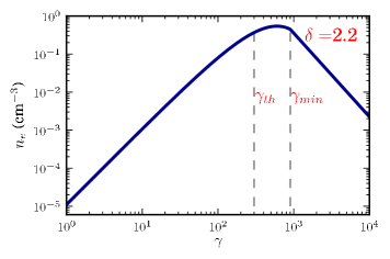
Figure 1.— The physical electron spectrum (see eq. 2) used for fitting synchrotron spectra directly to the data. Here $\gamma_{\hbox{\sixrm th}}=300$ and $\gamma_{\hbox{\sixrm min}}=900$ which are the fixed values used for all fits in this study. The value of $\epsilon$ is fixed to $(\gamma_{\hbox{\sixrm min}}/\gamma_{\hbox{\sixrm th}})^{2}\times exp(-\gamma_{\hbox{\sixrm min}}/\gamma_{\hbox{\sixrm th}})$.

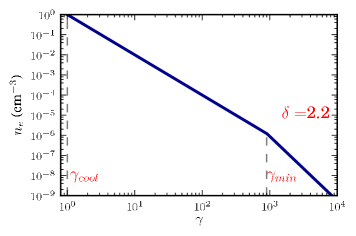
Figure 2.— The fast-cooled electron distribution with $\gamma_{cool}=1$ and $\gamma_{\hbox{\sixrm min}}=900$. A low-energy thermal distribution is excluded in this distribution because the synchrotron emission from the power-law form is already too broad for the typical $\nu F_{\nu}$ peak of the data and including a thermal distribution would smooth it further.

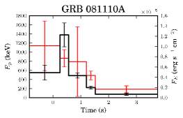
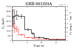
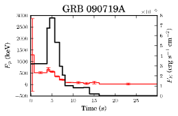
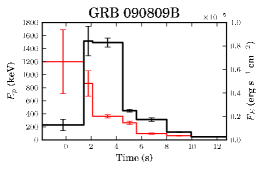
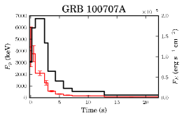
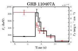
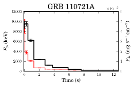
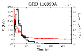
Figure 3.— The energy flux lightcurves of the synchrotron component for the entire sample (black curve). The integration range is from 10 keV - 40 MeV for all GRBs except GRB 081224A and GRB 110721A which are from 10 keV - 300 MeV. Superimposed is the slow-cooled synchrotron $E_{p}$ (see eq. 5) (red curve) demonstrating the hard to soft evolution of the bursts.

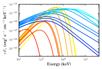
Figure 4.— The spectral evolution of GRB081224A is an example of the typical evolution observed for the entire sample. The synchrotron (from light blue to dark blue) and blackbody (from yellow to red) both evolve from hard to soft peak energies with time. For this GRB, the high-energy power-law corresponding to the electron spectral index does not evolve significantly over the duration of the burst.

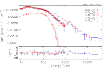
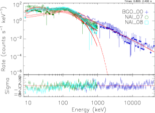
Figure 5.— A time bin of GRB 110721A (left panel) and GRB 100707A (right panel) demonstrating typical count spectra from the sample. Two extreme cases are shown: a subdominant and dominant blackbody component. The response has been convolved with synchrotron (eq. 3) and a blackbody to produce counts. The residuals from the fits indicate that the model is fitting the data well.

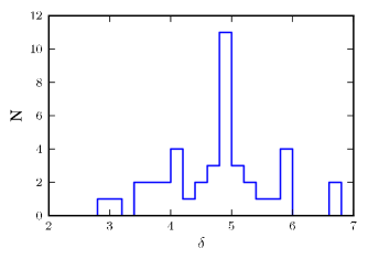
Figure 6.— The distribution of electron indices from the slow-cooling synchrotron fits. Only indices that were constrained are plotted. The distribution is broad but centered at $\delta=$5 which is much steeper than expected from simple relativistic shock acceleration.

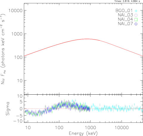
Figure 7.— The fast-cooled synchrotron fits are poor for nearly all of our sample because none of the spectra have a low-energy index as steep as $-$3/2. Therefore the fast-cooled synchrotron spectrum is too broad around the $\nu F_{\nu}$ peak as shown in this example spectrum.

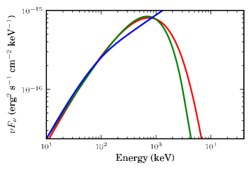
Figure 8.— An example time bin of GRB 110407A comparing the fitted $\nu F_{\nu}$ spectra of the Band Function (green), slow-cooled synchrotron (red), and fast-cooled synchrotron (blue). While the Band function and slow-cooled synchrotron fits resemble each other, the fast-cooled synchrotron fit is only able to fit the low-energy part of the spectrum. Because fast-cooled synchrotron has an index of $-$2/3 below the cooling frequency, the fitting engine pushes the value of E_∗ very high to fit the low-energy part of the spectrum resulting in a $-$3/2 index near the $\nu F_{\nu}$ peak. The high-energy power-law of the fast-cooling synchrotron spectrum is pushed out of the data energy window.

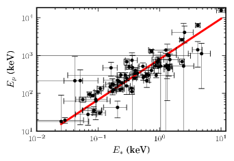
Figure 9.— Derived values of the parameter E_p (obtained using the Band function to fit GRB spectra), versus $E_{*}$ (obtained using an optically-thin non-thermal synchrotron to fit GRB spectra).

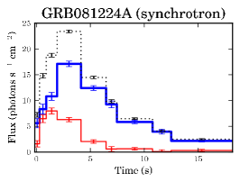
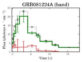
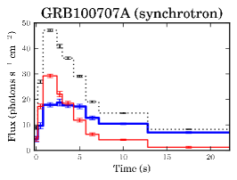
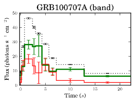
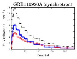
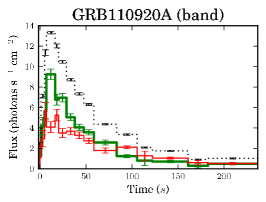
Figure 10.— A subset of flux lightcurves illustrating both the temporal structure of the different components and the advantages of using a physical model to deconvolve the detector response. The left column contains the lightcurves using synchrotron (blue thick line) and blackbody (red thin line) while the right column contains the lightcurves made from using the Band function (green thick line) and blackbody (red thin line). The total flux lightcurve (black dotted line) of both approaches are the same. The components have a very simple and constrained evolution when using synchrotron as the non-thermal component. This is potentially indicative that synchrotron is the actual emission mechanism and the response is being properly deconvolved. In contrast, the lightcurves where the Band function is used have large errors and the blackbody does not have a consistent evolution. (See the online version for color)

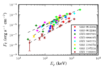
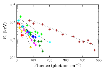
Figure 11.— The non-thermal emission of all of the bursts in the sample loosely follow $F_{E}$-$E_{p}$ and $E_{p}$-fluence relations. See Table 5 for the numerical results.

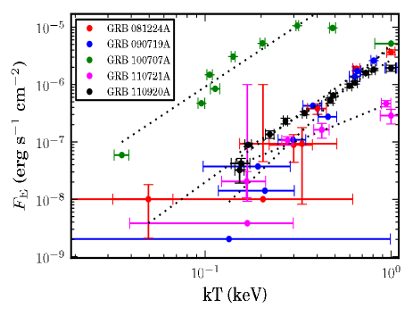
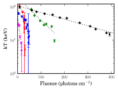
Figure 12.— The HIC and HFC correlations for the blackbody are separate from those derived from the synchrotron component. This adds more evidence for the presence of the component. However, the HIC for the blackbody is not q=4 as expected unless $\mathcal{R}$ varies as is observed.

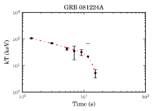
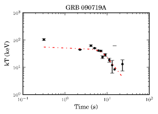
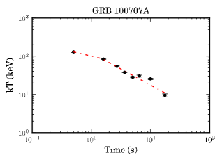
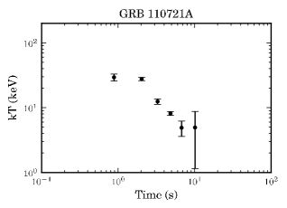
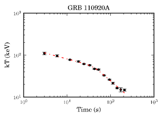
Figure 13.— The time evolution of kT for four of the GRBs in our sample. GRB110721A is shown without a fit because the coarse time binning used did not allow for constraining the fit parameters. However, in Axelsson et al. (2012), the evolution is shown to follow a broken power-law.

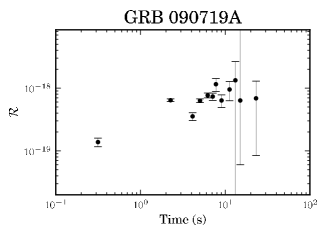
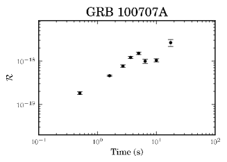
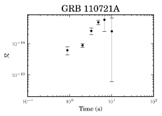
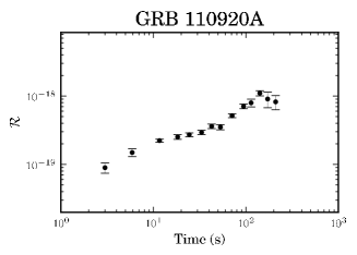
Figure 14.— The evolution of the $\mathcal{R}$ parameter is increases with time and shows no relation to the photon flux of the blackbody component.

GRB	Peak Flux (p/s/cm2)	Duration Analyzed (s)	Blackbody Component	LLE data
GRB 081110A	20.88	4.61	X	X
GRB 081224A	17.11	18.36	$\checkmark$	$\checkmark$
GRB 090719A	26.52	30.09	$\checkmark$	X
GRB 090809B	18.36	14.64	X	X
GRB 100707A	18.77	22.39	$\checkmark$	X
GRB 110407A	15.6	20.48	X	X
GRB 110721A	29.82	12.7	$\checkmark$	$\checkmark$
GRB 110920A	8.08	238.29	$\checkmark$	X

Table 1The GRBS in our sample. The peak fluxes were taken from the brightest bin of each GRB with a duration determined by Bayesian blocks.

Time Bin	Band C-Stat	Band+BB C-Stat	Synchrotron C-stat	Synchrotron+BB C-stat
-0.2-0.2	453	450	485	455
0.2-0.8	374	362	695	364
0.8-2.4	427	405	2546	487
2.4-3.0	408	400	903	413
3.0-4.3	431	415	1214	430
4.3-5.7	397	363	791	399
5.7-7.2	411	390	598	422
7.2-12.8	488	414	829	447
12.8-22.2	558	412	594	423

Table 2The time resolved C-Stat values for GRB100707A show that while the Band function and synchrotron models combined with a blackbody function both fit the data well, the non-thermal functions fit the data very differently when not combined with a blackbody. Specifically, where the blackbody is the brightest (Figures 10 and 10 intervals 2, 3, and 4) the Band function alone fits the data acceptably while the synchrotron model alone fits the data poorly. This shows that the flexibility of the Band function can mask the need for the blackbody component. The Band+blackbody fits actually fit the data better when the blackbody is very bright in this case. This is most likely due to the blackbody function (eq. 11) used is simplified and the actual emission may be broadened due to beaming effects that are only important to the fit when the blackbody is bright and the synchrotron fit is used. The Band function makes up for these effects by having a harder $\alpha$. We tested using an exponentially cutoff power-law combined with the synchrotron model and the fits were as good as those with the Band function. We will examine the use of a more realistic photosphere model in future work.

Time Bin	Band C-Stat	Band+BB C-Stat	Synchrotron C-stat	Synchrotron+BB C-stat	Fast C-stat	Fast+BB C-stat
-0.07-0.08	640	640	673	673	709	709
0.08-0.48	690	690	704	704	1088	1088
0.48-1.28	709	668	688	670	1654	957
1.28-2.78	887	761	838	770	1646	1041
2.78-3.78	678	642	655	643	797	666
3.78-5.88	648	631	677	634	694	660
5.88-7.63	729	728	733	721	773	724
7.63-12.63	932	693	693	692	756	698

Table 3The C-stat values for GRB 110721A. The significance of the addition of the blackbody is not as large as with GRB 100707A (Table 2) due to the weakness of the blackbody component. The fits for fast-cooled synchrotron are included to demonstrate the poor quality fits that are obtained both with fast-cooling synchrotron and fast-cooling synchrotron with a blackbody.

Time Bin	Band $\alpha$	Slow-cooled Synchrotron C-stat	Fast-cooled Synchrotron C-stat	$\Delta_{\rm C-stat}$
-5.38-2.82	-0.9	523	599	76
2.82-3.84	-0.7	507	604	97
3.84-4.86	-0.8	506	596	90
4.86-6.91	-1.0	534	626	92
6.91-9.98	-1.1	591	639	48
9.98-15.1	-1.5	494	494	0

Table 4For each time bin of GRB 110407A we examine the C-stat value of synchrotron and fast-cooled synchrotron. This GRB did not have a blackbody in its spectrum. While the Band function and slow-cooling synchrotron fit the spectrum well, fast-cooling synchrotron does not fit the spectrum unless Band $\alpha=-1.5$. In this case, the fast-cooled synchrotron peak energy was very unconstrained due to the curvature of the data being narrower than the photon model’s curvature.

GRB	Flux Index $q$	$\chi^{2}_{red}$	$\Phi_{0}$	$\chi^{2}_{red}$
GRB 081110A	2.32$\pm$0.4	0.6	97$\pm$23	0.4
GRB 081224A	1.74$\pm$0.1	1.5	253$\pm$23	0.3
GRB 090719A	1.14$\pm$0.07	0.98	245$\pm$17	1.2
GRB 09080B	1.58$\pm$0.05	8.0	188$\pm$9	1.0
GRB 100707A	1.04$\pm$0.02	1.2	444$\pm$24	7.3
GRB 110407A	1.72$\pm$0.20	0.5	214$\pm$32	4.2
GRB 110721A	1.08$\pm$0.03	14.4	269$\pm$13	15.4
GRB 110920A	1.37$\pm$0.06	0.5	669$\pm$33	1.2

Table 5Sample correlations for both flux and fluence for the synchrotron component.

Time Bin	Band-BB $\Delta_{C-stat}$	Synchrotron-BB $\Delta_{C-stat}$
-0.2-0.2	3	30
0.2-0.8	12	331
0.8-2.4	22	2059
2.4-3.0	8	490
3.0-4.3	16	784
4.3-5.7	34	392
5.7-7.2	21	176
7.2-12.8	74	382
12.8-22.2	146	171

Table 6The $\Delta_{C-stat}$ between the Band function and synchrotron model fits with and without the inclusion of a blackbody for GRB 100707A. The blackbody has a significantly larger impact on the fit when included with the synchrotron model.

Time Bin	Band-BB $\Delta_{C-stat}$	Synchrotron-BB $\Delta_{C-stat}$	Fast-BB $\Delta_{C-stat}$
-0.07-0.08	0	0	0
0.08-0.48	0	0	0
0.48-1.28	41	18	697
1.28-2.78	126	68	605
2.78-3.78	36	12	131
3.78-5.88	17	43	34
5.88-7.63	1	12	49
7.63-12.63	239	1	58

Table 7 The $\Delta_{C-stat}$ values for GRB 110721A tell a different story than GRB 100707A (Table 6), though both GRBs show a significant improvement in the fit when a blackbody is included. Even thought the fast-cooled fits showed extreme improvement with the inclusion of a blackbody, the fits are still poor compared with the slow-cooled model (See Table 3).

GRB	Flux Index	$\chi^{2}_{red}$	$\Phi_{0}$	$\chi^{2}_{red}$
GRB 081224A	2.3 $\pm$ 0.3	1.4	121 $\pm$ 13	9
GRB 090719A	2.8 $\pm$ 0.4	2.3	232 $\pm$ 23	3
GRB 100707A	2.2 $\pm$ 0.1	17.4	319 $\pm$ 8	28
GRB 110721A	1.3 $\pm$ 0.2	1.8	43 $\pm$ 3	5
GRB 110920A	2.0 $\pm$ 0.1	0.9	1147 $\pm$ 21.7	4

Table 8For the subset of bursts that have a strong blackbody component we compute the flux and fluence correlation for the blackbody.

GRB	$F_{bb}/F_{syn}$	$1^{st}$ Decay Index	$2^{nd}$ Decay Index	$\chi^{2}_{red}$
GRB 081224A	0.3	-0.6 $\pm$ 0.07	-20 $\pm$ 243	0.5
GRB 090719A	0.4	-0.1 $\pm$ 0.05	-2.0 $\pm$ 0.7	11.3
GRB 100707A	0.5	-0.4 $\pm$ 822749	-0.8 $\pm$ 0.03	22.7
GRB 110920A	0.8	-0.3 $\pm$ 0.03	-0.9 $\pm$ 0.04	2.0

Table 9The evolution of the blackbody follows a broken power-law. However, the coarse time bins recovered by the Bayesian blocks algorithm make it difficult to constrain the decay indices.

References

- Ackermann et al. (2012a) Ackermann, M. et al., 2012, ApJ, 745, 144.
- Ackermann et al. (2012b) Ackermann, M. et al., 2012, ApJ, 754, 121.
- Ackermann et al. (2012c) Ackermann, M. et al., 2012, ApJS, 203, 4.
- Arnaud, Smith, & Siemiginowska (2011) Arnaud K., Smith, R., & Siemiginowska, A. 2011, Handbook of X-ray Astronomy (Cambridge University Press)
- Axelsson et al. (2012) Axelsson, M. et al. 2012, ApJ, 757, L31.
- Asano, Inoue, & Mészáros (2009) Asano, K., Inoue, S., Mészáros, P. 2009, ApJ, 699, 953.
- Band et al. (1993) Band, D., Matteson, J., Ford, L., & Schaefer, B. 1993,ApJ, 413, 281.
- Baring, Ellison, & Jones (1995) Baring, M. G., Ellison, D. C., & Jones, F. C. 1995, Adv. Space. Res., 15, 397.
- Baring & Braby (2004) Baring, M. G. & Braby, M. 2004, ApJ, 613, 460.
- Baring (2006) Baring, M. G., 2006, Adv. Space. Res., 38, 1281.
- Baring (2011) Baring, M. G. 2011, Adv. Space. Res., 47, 1427.
- Beloborodov (2010) Beloborodov, A. M. 2010, MNRAS, 407, 1033.
- Beloborodov (2013) Beloborodov, A. M. 2013, ApJ, 764, 157
- Beniamini & Piran (2013) Beniamini, P., & Piran, T. 2013, ApJ, 769, 69
- Blumenthal & Gould (1970) Blumenthal, G. R. & Gould, R. J. 1970, Phys. Rev. 42, 237.
- Bos̆njak, Daigne, & Dubus (2009) Bos̆njak Z̆., Daigne F. & Dubus G. 2009, Astron. Astrophys., 498, 677.
- Borgonovo & Ryde (2001) Borgonovo, L. & Ryde F. 2001, ApJ, 548, 770.
- Burgess et al. (2011) Burgess, J. M. et al. 2011 ApJ, 741, 24.
- Cavallo & Rees (1978) Cavallo, G. & Rees, M. 1978, MNRAS, 183, 359.
- Cenko et al. (2011) Cenko et al. 2011, ApJ, 732, 29.
- Chiang & Dermer (1999) Chiang, J., & Dermer, C. D. 1999, ApJ, 512, 699
- Cohen et al. (1997) Cohen, E. et al. 1997, ApJ, 488, 330.
- Crider et al. (1999) Crider, A. et al. 1999, ApJ, 519, 206.
- Daigne & Mochkovitch (1998) Daigne, F. & Mochkovitch R. 1998 M.N.R.A.S., 296, 275.
- Daigne & Mochkovitch (2002) Daigne, F. & Mochkovitch, R. 2002 M.N.R.A.S., 336, 1271.
- Daigne, Bos̆njak, & Dubus (2011) Daigne F., Bos̆njak Z̆., & Dubus, G. 2011, Astron. Astrophys., 526, A110.
- Dermer et al. (2013) Dermer, C. D., Cerruti, M., Lott, B., Boisson, C., & Zech, A. 2013, arXiv:1304.6680
- Dermer (2004) Dermer, C. D. 2004, ApJ, 614, 284